

INTRODUCTION
Understanding the temporal and spatial distribution of parasite populations within and across host populations is fundamental for understanding the possible impact the respective parasite(s) may have on the evolutionary dynamics as well as population dynamics of the host species (Hudson et al. Reference Hudson, Rizzoli, Grenfell, Heesterbeek and Dobson2002). In addition, differences in parasite distributions among sub-groups in the host population can reveal important aspects of the parasite–host relationship (Hudson et al. Reference Hudson, Rizzoli, Grenfell, Heesterbeek and Dobson2002; Gurski and Ebbert, Reference Gurski and Ebbert2003). One of the most basic terms used to describe such a distribution is the ‘prevalence’, defined as the proportion of hosts infected by a parasite/disease in a population or sub-group at a given time (Rothman, Reference Rothman2012, p. 53–54). Prevalence may change over time as the factors that affect prevalence change (Rothman, Reference Rothman2012, p. 54). Few empirical studies of parasite prevalence in vertebrate populations span over longer time periods (but see Gulland et al. Reference Gulland, Albon, Pemberton, Moorcroft and Cluttonbrock1993; Hudson et al. Reference Hudson, Dobson and Newborn1998) and even fewer contain observations of temporal and spatial variations of prevalence in host metapopulations (Atkinson et al. Reference Atkinson, Dusek, Woods and Iko2000; Vogeli et al. Reference Vogeli, Lemus, Serrano, Blanco and Tella2011). Theoretical metapopulation models have shown that spatial fragmentation of a host population may increase the persistence (i.e. probability of extinction) of infective agents (Earn et al. Reference Earn, Rohani and Grenfell1998) and that persistence of an infective agent is determined by a balance between spatial, demographic and epidemiological components (Jesse and Heesterbeek, Reference Jesse and Heesterbeek2011). Although a theoretical framework for modelling parasites in a metapopulation exists, there is a need for empirical datasets preferably stretching over as many subpopulations and time periods as possible (Hudson et al. Reference Hudson, Rizzoli, Grenfell, Heesterbeek and Dobson2002). This need has become urgent due to an increase in number of fragmented populations as a result of human impact (Saunders et al. Reference Saunders, Hobbs and Margules1991). In such a system, parasites may play an important role in conservation of endangered populations (Hess, Reference Hess1996).
The parasite of interest in this study is the nematode worm Syngamus trachea. Syngamus trachea has a cosmopolitan distribution and has been found in most terrestrial bird genera (Yamaguti, Reference Yamaguti1961). In Norway the parasite has been recorded in several wild bird species (for list see Bakke, Reference Bakke1973). The parasite is known as ‘Gape worm’ in the domestic bird industry, where outbreaks have caused substantial problems (Atkinson et al. Reference Atkinson, Thomas and Hunter2008). Syngamus trachea has a life cycle that may include one paratenic host in addition to the final avian host. These paratenic hosts can be earthworms, snails or insects (Atkinson et al. Reference Atkinson, Thomas and Hunter2008). By eating one or more of these paratenic hosts containing an egg or larvae of S. trachea, the bird can become infected (Clapham, Reference Clapham1934). The larva makes its way from the stomach of the bird, through the blood vascular system to the lungs or trachea, where it then grows into an adult and finds a mate to copulate with (Atkinson et al. Reference Atkinson, Thomas and Hunter2008). The prepatent period in chickens (Gallus gallus) is 12–17 days and the adults can live 2–4 months (Barus, Reference Barus1966b). After a female and male are joined, they mate and the female releases eggs which are coughed up by the host and then swallowed (Atkinson et al. Reference Atkinson, Thomas and Hunter2008). The eggs then pass out in the feces and may enter another bird either directly or via a paratenic host (Clapham, Reference Clapham1934; Bakke, Reference Bakke1973). The adult male parasite is 3–5 mm long and the adult female is 17–30 mm long (Barus and Blazek, Reference Barus and Blazek1965). After copulation the adult male and female are permanently attached to each other in a Y-shape. The parasites feed on blood in the trachea tissue causing mechanical damage, anaemia, inflammation and excess mucus production. The birds that are infected may develop symptoms consisting of gasping, wheezing and shaking of the head. This discomfort may affect food uptake, and combined with the blood loss, may cause death (Atkinson et al. Reference Atkinson, Thomas and Hunter2008).
The house sparrow is a small passerine bird with a global distribution, and is widely spread in the northern hemisphere (Anderson, Reference Anderson2006). The house sparrows along the coast of northern Norway live in close association with human settlements, in particular dairy farms. This is strongly reflected in the behaviour ecology and foraging patterns of the species. During the winter a substantial part of the diet consists of concentrated cattle food, and seeds from cultivated crops (Anderson, Reference Anderson2006). In the summer season the house sparrows forage outdoors, to a large extent, on different types of seeds and insects (Anderson, Reference Anderson2006). Sparrows living on farms most frequently place their nests inside cowsheds and barns. House sparrows also shelter inside farm buildings when the weather is harsh (especially in winter) (Summers-Smith, 1988). Because of the species' sedentary nature and the high proportion of individually recognizable birds in our metapopulation, we have the opportunity to track individual movement between islands in the study area (Pärn et al. Reference Pärn, Jensen, Ringsby and Sæther2009, Reference Pärn, Ringsby, Jensen and Sæther2012).
In the present study we explore the prevalence of the parasite S. trachea in a metapopulation of house sparrows (Passer domesticus) in the Helgeland archipelago in northern Norway over a 4-year period. This is a metapopulation that has been thoroughly studied at an individual-based level since 1993 and offers a unique opportunity to shed light on parasite ecology in a spatially distributed population of wild hosts. Our aim was to investigate whether the prevalence of S. trachea varied in time and/or space on the respective islands. We also investigated the possibility that prevalence patterns could be explained by differences among the demographic groups in the respective populations.
METHODS
Study area
The study was carried out in an archipelago consisting of 18 islands in the Helgeland district in northern Norway. The house sparrows on these islands have been studied on an individual-based level by capture–mark–recapture methods since 1993 (e.g. Sæther et al. Reference Sæther, Ringsby, Bakke and Solberg1999; Ringsby et al. Reference Ringsby, Sæther, Tufto, Jensen and Solberg2002; Jensen et al. Reference Jensen, Steinsland, Ringsby and Sæther2008). In this study we focus on four of the main study islands (Aldra, Gjerøy, Hestmannøy and IndreKvarøy). On these islands a high proportion of the individuals have been individually marked (>90%), the annual recapture probability is high (>0·7, see Billing et al. Reference Billing, Lee, Skjelseth, Borg, Hale, Slate, Pärn, Ringsby, Sæther and Jensen2012), and fecal samples have been collected since 2007. These are islands where the birds live mainly in connection with farms. House sparrows have been captured, marked and sampled several times during their lifetime.
Sample collection and analysis
During field work house sparrows were captured using mist-nets. For the purpose of obtaining a fecal sample they were thereafter placed in paper bags with a small hole at the top to prevent asphyxiation. After approximately 10–15 min in the paper bag, a fecal sample had usually been obtained. According to procedures described in Gjerde (Reference Gjerde and Veterinærhøyskole2007) each fecal sample was placed in 1 mL of MilliQ H2O in a 1·5 mL cryo-tube. Samples were then kept refrigerated (at between 1 and 8 °C) until analysed. 1150 fecal samples were collected during the breeding seasons 2007–2010 (1 May–15 August) from 752 birds. In addition, we also collected samples from one of the study islands (Hestmannøy) in the winters (February–March) of 2009 (32 samples) and 2010 (46 samples).
To individually mark each bird, they were assigned unique individual ring codes consisting of a numbered metal ring and three additional plastic colour rings; two rings on each tarsus. In this way individual birds could later be identified by observation/capture to determine for example age and dispersal distance. When captured, the sex was determined for adult birds based on plumage characteristics. Individuals were also categorized into juveniles (birds younger than one year) and adults (birds in their first breeding season or older). (See Ringsby et al. Reference Ringsby, Sæther, Tufto, Jensen and Solberg2002; Jensen et al. Reference Jensen, Steinsland, Ringsby and Sæther2008; Pärn et al. Reference Pärn, Jensen, Ringsby and Sæther2009, for further description of field work.)
To analyse parasite load the fecal samples were first centrifuged at 605 g for 60 s (Eppendorf MiniSpin®). The supernatant of MilliQ H2O was then removed and replaced with sucrose-saturated water. The samples were centrifuged again at 151 g for 45 s, and placed in a Mcmaster/Whitlock counting chamber under a microscope (Leica, model: DMLS). Eggs of S. trachea were identified by their size (approximately: 80–100 μm×50–60 μm), shape (bipolar) and visible opercula at both ends (Atkinson et al. Reference Atkinson, Thomas and Hunter2008). The number of S. trachea eggs were counted by eye using a handheld Redington Counter. Detection of eggs from S. trachea in bird feces has been shown to be a reliable and stable way of monitoring infection in populations (Barus Reference Barus1966b, Reference Barus1966c).
Statistical analyses
The response variable used in our statistical analyses was infection status. If eggs of S. trachea were found in a fecal sample the individual's infection status was defined as 1 (i.e. ‘infected’). Correspondingly, if eggs were not detected in the feces the individual was given an infection status of 0 (i.e. zero eggs).
Island was the only spatial explanatory variable used in the analyses. Temporal explanatory variables were year and seasonal day number (SDN). The SDN indicated which day during the season a bird was sampled, where day 1 was set to 1 May. The SDN variable was then centred on zero (mean = 0) in order to increase interpretability of possible interactions (Aiken and West, Reference Aiken and West1991).
Demographic explanatory variables consisted of age-class (adult/juveniles) and life-stage group (LSG: juvenile, adult male, adult female). We were not able to include sex of juveniles in the study due to difficulties in confidently determining sex of birds that had not acquired their adult plumage.
All analyses were done using the statistical software package R version 2.14.1 (R Development Core Team 2012). We applied generalized linear mixed models (package glmmADMB version 0.7.2.5) with a Bernoulli response variable and a logit link function in our investigation of prevalence. Because some birds (N = 213) were caught more than once during a respective season we used individual identity as a random factor in order to avoid pseudoreplication.
To evaluate the effect of our explanatory variables we applied multiple model comparisons using an information-theoretic approach based on Akaike information criterion corrected for small sample sizes (AICc), which penalizes models with a high number of parameters relative to sample size (Burnham and Anderson, Reference Burnham and Anderson2002).
In all our models we included the first-order term of SDN due to the a priori assumption that prevalence of S. trachea varied significantly within years (Barus, Reference Barus1966c). All models were created manually and explored all possible 2-way interactions between explanatory variables. We separated our analysis into two sections in order to reduce the number of potential models. In the first section, we ran a set of models that included all our spatial and temporal explanatory variables (SDN, year and island). The best model according to AICc was then used as the base model in the second section of analyses. In the second section of analyses, we investigated if demographic variables such as age-class and LSG could further improve the fit of the best model selected in the first section of analyses. Because the two demographic variables (age-classes and LSG) contained much of the same information, they were not included in the same models.
When including a random effect u representing heterogeneity between individuals the prevalence p becomes a random variable. For a given value of the random effect u (e.g. within a given individual), the relationship between the prevalence p and covariates X of interests becomes:  $p = {\rm logit}^{ - 1} (X\beta + u)$. Here our interest, however, is in the relationship between mean prevalence p of a randomly selected individual and the covariates X, which is given by
 $$E(\,p) = \int {{\rm logit}} ^{ - 1} (X\beta + u)\ f\,(u)du,$$
where f(u) is the density function of the random effect u (Agresti, Reference Agresti2002, p. 498). This relationship (sometimes referred to as the marginal model) has a considerably shallower slope than the relationship between p and X conditional on u (the conditional model, see Agresti (Reference Agresti2002), section 12·2·2 for an in-depth discussion). We computed the above integral using adaptive quadrature numerical integration (function integrate in R).
RESULTS
First section of analyses
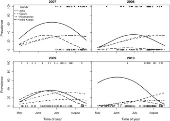
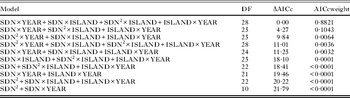
When analysing whether the prevalence of S. trachea was influenced by spatial and temporal variables the model comparisons (Table 1) showed that the model which received most support given the data included all the main effects of all the explanatory variables (island, SDN, SDN2 and year), along with the interactions year×SDN, island×SDN, island×SDN2 and island×year (see Appendix I for details). This model had an AICc value of 866·94 which was 4·27 lower than the second-best model, suggesting that the highest ranked model was considerably better than the second-best model. In addition, the AICc weight of the highest ranked model indicated that there was an 88·21% probability that this model was the best given the data and the set of candidate models. The highest ranked model showed that a general difference in prevalence existed both between and within years and between and within islands (see Fig. 1).
Graphical presentation of predictions from the best generalized linear mixed model describing prevalence of the parasite Syngamus trachea in an insular metapopulation of house sparrows on the coast of Helgeland in northern Norway. The response variable in the model was the binary occurrence (1) or absence (0) of eggs in feces of house sparrows. Individual identity was used as a random factor. Data were obtained from fecal samples from four islands during the breeding seasons of the years 2007–2010. The predicted relationships from the model between season and prevalence for the four islands are plotted as lines. Sample sizes are shown as ‘sunflower’ points denoting number of negative (individual prevalence = 0%) and positive (individual prevalence = 100%) samples, respectively.

Top 10 (of 44) models in an AICc comparison of generalized linear mixed models explaining prevalence of the parasite Syngamus trachea in a metapopulation of house sparrows on the coast of Helgeland in northern Norway. All models included individual identity as a random factor. Data were collected on four islands during the breeding season (1 May–17 August) in the years 2007–2010. SDN is a continuous variable indicating which day during the breeding season a bird was sampled. Interaction terms between two variables are denoted A×B. Note that models with interactions also include the main effects of A and B

The inclusion of the second-order term of SDN as a main effect in the highest ranked model, pointed to a seasonal peak of prevalence within years on our islands. The mean prevalence appeared to increase during the breeding season to a general maximum in late summer and then decline towards autumn (see Fig. 1). Samples taken from Hestmannøy in the winters of 2009 (N = 32) and 2010 (N = 46) indicated a prevalence of only 3 and 0%, respectively, which strongly suggest that a seasonal peak pattern in the prevalence of S. trachea was present.
The main effect of year, showed an overall difference in prevalence between years (see Fig. 1). The main effect of islands indicated that the mean prevalence in the total sampling period was highest on Aldra and lowest on Gjerøy (see Fig. 1).
The interactions between the first-order term of SDN and year/island (Table 1) suggested that the rate of change in prevalence with SDN differed both among years and islands, respectively. In addition, the interaction between the second-order term of SDN and island (Table 1) points to a difference in date for the ‘peak’ prevalence between islands (see Fig. 1).
The interaction between island and year indicated that the yearly change in prevalence was not the same on all islands. For example, at Hestmannøy the mean prevalence decreased successively each year, while on Aldra the mean prevalence decreased from 2007 to 2009 and then increased in 2010 compared with previous years (see Fig. 1).
Second section of analyses
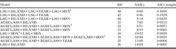
The extension of the highest ranked model from our first section of analyses by inclusion of demographic variables resulted in an improvement of the model (see Table 2). Here, the highest ranked model (see Appendix II for details) had an AICc value of 849·07 which was only 0·96 lower than the second-best model (Table 2). This suggests that the second-best model also should be viewed as a good model when interpreting the results. Accordingly, the AICc weights strongly supported the explanative properties of the two highest ranked models (Table 2). The highest ranked model from our first section of analyses obtained an AICc value which was 17·86 higher than the new highest ranking model, given the data and the alternative models (see Appendix II for details).
Top 10 (of 31) models in an AICc comparison of generalized linear mixed models explaining prevalence of the parasite Syngamus trachea in a metapopulation of house sparrows on the coast of Helgeland in northern Norway. All models included individual identity as a random factor. Data were collected on four islands during the breeding season (1 May–17 August) in the years 2007–2010. SDN is a continuous variable indicating which day during the breeding season a bird was sampled. Age class is a categorical variable dividing house sparrows into juveniles and adults. LSG is a categorical variable denoting the three main demographic groups in house sparrow populations: adult males, adult females and juveniles. All models also contain the terms from the best model in a previous model comparison (SDN×YEAR+SDN×ISLAND+SDN2×ISLAND+ISLAND×YEAR, see Table 1). Interaction terms between two variables are denoted A×B. Note that models with interactions also include the main effects of A and B

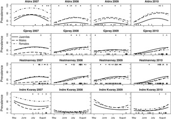
The two highest ranked models in the second section of analyses included the main effects of LSG, year and island along with the interactions LSG×year and LSG×island. The highest ranked model also contained the interaction LSG×SDN2. The main effect of LSG suggested differences in prevalence between the three life-stage groups. In general, juveniles appeared to have the highest mean prevalence and adult males the lowest (see Fig. 2).The interaction terms indicated that these differences were not the same between years or islands, and suggested that the peak date in prevalence may differ between the three groups (see Fig. 2).
Graphical presentation of predictions from the best generalized linear mixed model describing prevalence of the parasite Syngamus trachea in an insular metapopulation of house sparrows on the coast of Helgeland in northern Norway. The response variable in the model was the binary occurrence (1) or absence (0) of eggs in feces of house sparrows of different life-stage groups (juvenile, adult female or adult male). Individual identity was used as a random factor. Data were obtained from fecal samples from four islands during the breeding seasons of the years 2007–2010. Sample sizes are shown as ‘sunflower’ points denoting number of negative (individual prevalence=0%) and positive (individual prevalence=100%) samples, respectively.

DISCUSSION
This study demonstrates that the prevalence pattern of a parasite in a metapopulation of hosts can become quite complex and vary in time, space and among sub-groups of hosts. To our knowledge, this is the first empirical study to show such detailed prevalence dynamics of a macroparasite in a metapopulation of wild avian hosts. Furthermore, our results emphasize the importance of establishing a sampling regime that accounts for seasonal variation in prevalence throughout the year, over several years and spatially among populations in order to achieve a more complete picture of parasite–host dynamics.
The within-year variation in prevalence of S. trachea is supported by studies conducted by Barus (Reference Barus1966c). He also found a peak in prevalence of the parasite on poultry farms in Germany in late summer. In concordance with our results Barus (Reference Barus1966b) also found that prevalences dropped to nearly zero during winter time and attributed this pattern to climatic patterns, especially temperature, throughout the year. This link was investigated in another study by Barus (Reference Barus1966a) with experimental observations of egg development time of S. trachea from embryo to invasive stage larvae. It was then found that embryos did not develop when the temperature was 16 °C or lower. Development time dropped with increasing temperature and reached an ‘optimum’ of c. 7 days at 29 °C. This may indicate an important limiting factor for S. trachea in our study system which is located on the Arctic Circle. In wintertime, the temperature inside or outside the barns at Helgeland does not exceed the minimal temperature of 16 °C in a normal year (Ringsby et al. unpublished results). In summertime, the mean daily temperature recorded by the Norwegian Meteorological Institute's weather stations in the area usually does not exceed 16 °C (Ringsby et al. Reference Ringsby, Sæther, Tufto, Jensen and Solberg2002). Nevertheless, the temperature often exceeds 16 °C in sunlight and under the tin sheet roofs on barns at Helgeland (Ringsby et al. unpublished results). Furthermore, there may be several factors other than temperature affecting seasonal parasite prevalence in our population(s), such as for example host density and inter-individual variation between host age-classes and sexes in energy available for defence against the parasite that may change over the breeding season (e.g. Hudson et al. Reference Hudson, Rizzoli, Grenfell, Heesterbeek and Dobson2002).
The highest ranked model from our first section of analyses also indicated that differences between years was an important contributor to explaining prevalence patterns. Inter-annual variation in prevalence has been found in several other parasite–host systems (Weatherhead and Bennett, Reference Weatherhead and Bennett1991; Thompson et al. Reference Thompson, Corpe and Reid1998; Macdonald et al. Reference Macdonald, Anwar, Newman, Woodroffe and Johnson1999), and may be explained by several factors. For example, climate (Kutz et al. Reference Kutz, Hoberg, Polley and Jenkins2005), host population densities (Arneberg, Reference Arneberg2001) and vector availability (Weatherhead and Bennett, Reference Weatherhead and Bennett1991) may have an effect on the parasite prevalence in a given year. To our knowledge, no ad libitum distributions of antiparasitic substances or relevant treatments were implemented by local farmers in the study period. In general, use of antiparasitic treatments/substances is strictly regulated in Norwegian agriculture (NOMA, 2001). Disentangling what may have caused the temporal patterns observed in this study should however be a topic for future work.
Our results also indicate that the yearly and within-year change in prevalence was not the same on all islands. This may be due to differences in local abiotic conditions among islands (patches), difference in paratenic host availability, or could be caused by genetic differences between islands in either host or parasite. For example, it seems possible that there may be differences between our island populations with respect to genetic variation in the immune system. Accordingly, the island of Aldra, with the highest prevalence of S. trachea, has a population history involving a recent population bottleneck and high level of inbreeding (Billing et al. Reference Billing, Lee, Skjelseth, Borg, Hale, Slate, Pärn, Ringsby, Sæther and Jensen2012), low effective population size (Engen et al. 2007, Baalsrud et al. in review), and low level of ‘neutral’ genetic variation (Jensen et al. Reference Jensen, Bremset, Ringsby and Sæther2007, in review). Although based on very small sample sizes (five individual sparrows from each island population), a recent study suggested however that the level of variation at major histocompatibility complex genes which are important in the vertebrate immune system was similar on Aldra and Hestmannøy (Borg et al. Reference Borg, Pedersen, Jensen and Westerdahl2011). Other studies have shown that inbreeding may affect parasite prevalence. This was for example found by Ilmonen et al. (Reference Ilmonen, Penn, Damjanovich, Clarke, Lamborn, Morrison, Ghotbi and Potts2008) who showed that inbreeding could have a significant negative effect on host (Musmusculus domesticus) resistance to Salmonella. Alternatively, the differences between islands may be caused by different strains/sub-species of S. trachea inhabiting our islands. Spatial differences in strains/sub-species of parasites have been found in other study systems (Bensch and Akesson, Reference Bensch and Akesson2003; Gaspar da Silva et al. Reference Gaspar da Silva, Barton, Bunbury, Lunness, Bell and Tyler2007; Wood et al. Reference Wood, Cosgrove, Wilkin, Knowles, Day and Sheldon2007; Henriques-Gil et al. Reference Henriques-Gil, Haro, Izquierdo, Fenoy and del Aguila2010). There may also be complex interactions between S. trachea and other local parasites. We have detected several other parasites inhabiting our study populations (Holand et al. unpublished results), both from our fecal samples (endoparasites: Isospora spp., Capillaria spp., Choanotaenia spp.) and visual inspection of house sparrows (ectoparasites: Hippoboscidae spp., Ornithonyssus spp., Ceratophyllus spp.). Oocysts of Coccidian (Isospora spp.) species were found in 59% of fecal samples while eggs of Capillaria spp. and Choanotaenia spp. were only found in 0·2 and 0·09% of fecal samples, respectively. Interactions between different parasite species have been demonstrated in other studies (see Poulin, Reference Poulin2007). However, more detailed studies are needed in order to investigate the relative importance of alternative causes for the different patterns in prevalence between our islands.
The second section of our analyses revealed that the difference in prevalence between discrete demographic groups explained a substantial part of the total variation in prevalence. Life-stage group (LSG: juvenile, adult male, adult female) seemed to explain more of the variation in prevalence than the simpler age class variable (adult/juvenile). This was partly due to a general difference between the three groups, but also due to considerable differences between the groups in both time and space (Fig. 2). Although adult males and females generally had a lower prevalence compared with juveniles, this pattern was opposite in some years on some islands. The apparent difference in prevalence and the relationship between date and prevalence between the demographic groups may be due to unequal exposure to infective stage of the parasite. For instance, Ringsby et al. (Reference Ringsby, Berge, Sæther and Jensen2009) showed that females in general have a higher feeding rate of nestlings compared with males. If the parasite is transmitted through food items (insects etc.) one may expect the females and nestlings (of which some survive to become juveniles) to show similarities in prevalence (see Zuk and McKean, Reference Zuk and McKean1996). On the other hand, differences in prevalence may be caused by differences in immunity. Other studies (Clapham, Reference Clapham1934; Bakke, Reference Bakke1973; Wissler and Halvorsen, Reference Wissler and Halvorsen1975) have found higher prevalence of S. trachea in juvenile birds. This pattern has been attributed to acquired immunity with age (Atkinson et al. Reference Atkinson, Thomas and Hunter2008). If this is the case in our populations, one might expect to see a higher prevalence in juveniles compared with adults and that birds rarely get infected more than once. Indeed, out of the 121 birds sampled in more than one year, only five birds were shown to be infected in more than one year. This seems to indicate that infection by S. trachea is generally a ‘once in a lifetime’ event for our house sparrows. All these possibilities along with several others (see Zuk and McKean, Reference Zuk and McKean1996; McCurdy et al. Reference McCurdy, Shutler, Mullie and Forbes1998; Hudson et al. Reference Hudson, Rizzoli, Grenfell, Heesterbeek and Dobson2002; Lachish et al. Reference Lachish, Knowles, Alves, Wood and Sheldon2011) may explain the demographic prevalence patterns observed in our study.
Investigating and understanding parasite prevalence-patterns in space and time is a fundamental step in determining the possible evolutionary and ecological effects parasites may have on host populations. In natural populations, this is however a relatively novel area of research but one that probably will increase in importance as the climate changes and populations are exposed to novel parasites, or effects of parasites are amplified by shortened development time, longer transmission season and reduced generation times expected as a consequence of rising temperatures (see Kutz et al. Reference Kutz, Hoberg, Polley and Jenkins2005).
ACKNOWLEDGEMENTS
We would like to thank Lars Erik Andersen, Helle Tessand Baalsrud, Johan Henrik Hårdensson Berntsen, Roger Dahl, Ole Roar Davidsen, Ingerid J. Hagen, Atle Torvik Kristiansen, Thomas Kvalnes, Aline M. Lee, Siri Johansen Monkan, Ane M. Myhre and Henrik Pärn for helping to collect fecal samples. We are also grateful to everyone at Centre for Biodiversity Dynamics (CBD) at the Department of Biology, NTNU, for helpful comments and help with statistics in R and lab work. Finally we would like to thank Bjørn Gjerde at the Veterinary Institute in Oslo for taking time out of his busy day in order to teach Håkon Holand the fine art of fecal examination.
FINANCIAL SUPPORT
This study was funded by the Norwegian Research Council and the Norwegian University of Science and Technology. The research was carried out in accordance with permits from the Norwegian Directorate for Nature Management and the Bird Ringing Centre at Stavanger Museum, Norway.
Appendix I
Table listing the estimates and standard errors from the top model in an AICc comparison of generalized linear mixed models explaining prevalence of the parasite Syngamus trachea in a metapopulation of house sparrows on the coast of Helgeland in northern Norway. All models included individual identity as a random factor. Data were collected on four islands during the breeding season (1 May–17 August) in the years 2007–2010. SDN is a continuous variable indicating which day during the breeding season a bird was sampled. Interaction terms between two variables are denoted A×B. Intercept contains the estimates of the year 2007 and the island Gjerøy

Table listing the 44 models used in an AICc comparison of generalized linear mixed models explaining prevalence of the parasite Syngamus trachea in a metapopulation of house sparrows on the coast of Helgeland in northern Norway. All models included individual identity as a random factor. Data were collected on four islands during the breeding season (1 May–17 August) in the years 2007–2010. SDN is a continuous variable indicating which day during the breeding season a bird was sampled. Interaction terms between two variables are denoted A×B. Note that models with interactions also include the main effects of A and B

Appendix II
Table listing the estimates and standard errors from the top model in an AICc comparison of generalized linear mixed models explaining prevalence of the parasite Syngamus trachea in a metapopulation of house sparrows on the coast of Helgeland in northern Norway. All models included individual identity as a random factor. Data were collected on four islands during the breeding season (1 May–17 August) in the years 2007–2010. SDN is a continuous variable indicating which day during the breeding season a bird was sampled. LSG is a categorical variable denoting the three main demographic groups in house sparrow populations: adult males, adult females and juveniles. Interaction terms between two variables are denoted A×B. Note that models with interactions also include the main effects of A and B. Intercept contains the estimates of the year 2007, the island Gjerøy and adult females

Table listing the 31 models used in an AICc comparison of generalized linear mixed models explaining prevalence of the parasite Syngamus trachea in a metapopulation of house sparrows on the coast of Helgeland in northern Norway. All models included individual identity as a random factor. Data were collected on four islands during the breeding season (1 May–17 August) in the years 2007–2010. SDN is a continuous variable indicating which day during the breeding season a bird was sampled. Age class is a categorical variable dividing house sparrows into juveniles and adults. LSG is a categorical variable denoting the three main demographic groups in house sparrow populations: adult males, adult females and juveniles. All models also contain the terms from the best model in a previous model comparison (SDN×YEAR+SDN×ISLAND+SDN2×ISLAND+ ISLAND×YEAR, see Table 1). Interaction terms between two variables are denoted A×B. Note that models with interactions also include the main effects of A and B