Introduction

Glaciers ending in bodies of water lose ice by calving. Calving occurs both from floating ice shelves and from valley glaciers that remain grounded essentially all the way to their termini. The blocks of ice thus lost range in size from individual ice crystals separated from a calving face by melting along grain boundaries to tabular icebergs hundreds of square kilometers in area that break off from ice shelves. Melting may influence the calving process by altering the shape of a calving face and is itself included implicitly in most calculations of calving speed. The water into which glaciers calve may be either salty or fresh and either stable or mixed by river and tidal currents, all of which affect melt rates. Given these complexities, it is not surprising that no known theoretical or empirical rule governs the rate at which these processes, combined, result in ice loss from calving faces.

In this paper, we limit our discussion to grounded valley glaciers calving into tidal salt-water fjords and inlets. For this restricted calving environment, an empirical relationship between calving speed and water depth has been advanced, but the fundamental physical processes that govern the calving rate are still poorly understood. Our objective herein is to propose some such processes that could account for the empirically observed approximately linear increase in calving rate with water depth.

Calving of grounded glaciers is of considerable interest: it can be responsible for icebergs that threaten shipping; it affects the way in which valley glaciers react when dams raise lake levels near their termini (Reference Funk and RöthlisbergerFunk and Röthlisberger, 1989; Reference Hooke, Laumann and KennettHooke and others, 1989); and if ice sheets in Greenland and Antarctica begin to disintegrate as a result of climatic warming, calving will control the rate of collapse. Initially, calving in Antarctica will be largely from ice shelves, but as these vanish, grounded ice streams, resembling tidewater glaciers, will play an increasingly important role.

Background

In studies of Alaskan tidewater glaciers, Reference Brown, Meier and PostBrown and others (1982) found a strong correlation between mean annual calving speed, u _c, and the average depth of the water body along the calving face, h _w, but the physical reasons for this were unclear. They also considered the possibility that u _c might be related to accumulated strain, ice speed, ice thickness, effective pressure, state of the tide, water temperature and the volume of subglacial runoff (Reference Brown, Meier and PostBrown and others, 1982, p. C8). Intuitively, some dependence of calving speed on some of these parameters is likely, but they found “no direct evidence that these variables need to be separated explicitly”. Reference Meier and ReehMeier (1994) incorporated 14 years of recent data from Columbia Glacier into Brown and others’ dataset and found that the new data were generally consistent with the earlier values, except for the last 2 years, when the calving rate may have been affected by floating.

Calving speeds of polar glaciers in West Greenland and Svalbard and of temperate glaciers ending in fresh-water lakes are also proportional to water depth. However, the calving speeds of the polar glaciers are about one-third of those of Alaskan glaciers in water of similar depth (Reference Pelto and WarrenPelto and Warren, 1991), and those of temperate glaciers ending in fresh water are only about one-tenth of those of their Alaskan counterparts (Reference Funk and RöthlisbergerFunk and Rothlisberger, 1989). Reeh (cited by Meier, 1993) compiled data for floating polythermal glaciers in Greenland and found that u _c was proportional to ice thickness, but calving rates were only about one-fifth of those of grounded temperate Alaskan glaciers.

In contrast, Reference SikoniaSikonia (1982) found that over time-spans of weeks to months, calving rates in an embayment in the calving face of Columbia Glacier showed little relation to local water depth. However, he and Reference Sikonia and PostSikonia and Post (1979) found that over these time-spans u _c was directly related to water discharge in the nearby Knik River and inversely related to the effective pressure at the bed. We will return to this later.

Reference Hughes and NakagawaHughes and Nakagawa (1989) have suggested that bending shear controls calving speed. Observations of a vertical ice face on dry land on Deception Island showed that as the top of the face moved forward faster than the bottom, shear zones developed along arcuate surfaces much as the pages of a book shear past one another if the binding is held fixed on a horizontal surface and the pages are bent to the side. Failure eventually occurs along surfaces that follow shear zones downward and then, near the base, veer outward toward the face at about 45°, following a plane of maximum shear stress. This type of failure is probably less important in the tongue of a pervasively fractured tidewater glacier.

Reference HughesHughes (1992), expanding on these ideas, developed a physically based calving model, using beam theory. Interestingly, agreement with observation is reasonably good. However, in contrast to the situation with calving tidewater glaciers: (1) stresses are assumed to be distributed linearly as in an elastic beam; (2) calving blocks are assumed to extend over the full height of the calving face, including the submerged part; (3) the calving speed calculated is the speed of movement of the top of individual calving blocks at the moment of failure; and (4) the stress field assumed is not appropriate where the water is deep and the glacier approaches flotation. Consequently, Hughes’ approach does not appear to be appropriate for the present problem.

Role of Crevassing

Reference Van der VeenVan der Veen (1996) proposed a quite different model of calving. He believes that when a tidewater glacier thins sufficiently, though remaining grounded, it becomes weak and fails (Reference Van der VeenVan der Veen, 1996, p.382). Reference HookeHooke (1983; see Reference Meier and ReehMeier, 1994) suggested that such weakening might be due to pervasive fracturing resulting from high longitudinal strain rates, and indeed longitudinal strain rates in a tidewater glacier are likely to increase as the glacier approaches flotation. Reference HookeHooke (1983), Reference Meier and ReehMeier (1994) and Reference Van der VeenVan der Veen (1996, fig. 3) have all found weak correlations between strain rate and calving speed. In the Van der Veen model, the continuum that is failing is rather like a pile of irregular, weakly bonded blocks of soil being pushed from behind, as by a bulldozer: as the front of the pile becomes oversteepened, blocks collapse off of it. In this model, the calving speed depends upon the flux of ice to the calving face, much as the rate at which water comes out of a pitcher depends upon the rate at which the pitcher is tilted.

Reference PostPost (1997) argues that the absence of icebergs of significant size in the forebay of Columbia Glacier today is evidence for such pervasive fracturing at depth. Similarly, Reference VenterisVenteris (1997) found that the divergence of the velocity field at the surface of Columbia Glacier suggested a thinning rate well in excess of that measured. He attributed the discrepancy to pervasive internal and bottom crevassing.

Role of Glacier Speed

If u _c depends upon the flux of ice to the calving face, it will correlate closely with the mean ice speed at the terminus, u _i, which, in turn, depends on factors such as fjord geometry and depth (Reference Van der VeenVan der Veen, 1996). Indeed, there is a strong correlation between u _c and u _i, but this may be largely because u _c is normally determined by measuring u _i and subtracting the rate of change in glacier length, dL/dt, thus:

(1)

(Note that u _c thus encompasses all ice-loss processes at the margin including, for example, melt and sublimation as well as failure of small and large ice blocks.) Because dL/dt is small compared with u _i under most conditions, there is bound to be a good correlation between u _c and u _i, as Reference Van der VeenVan der Veen (1996) has noted.

Because u _c is determined in this way, one may argue, as Reference Van der VeenVan der Veen (1996, p. 381) appears to, that it is circular to use the correlation between u _i and u _c as support for a physical relation between these two variables, or between one or both of them and a third variable, such as water depth. If it were possible to measure u _c independently, however, circularity would no longer be of concern. In short, the fact that the measurement of u _c is indirect and involves measuring u _i does not detract from the real possibility that u _c is somehow physically related to u _i.

Supporting Van der Veen’s model are data spanning about 50 years that suggest that at the terminus of Hasbreen in Svalbard, u _c and u _i have indeed varied roughly synchronously, although the water depth has remained nearly constant (Reference Jania and KaczmarskaJania and Kaczmarska, 1997). Unfortunately, this dataset is small, with some values representing averages over as much as 20 years, so the result must be viewed as only suggestive. Jania and Kaczmarska also note that on an annual basis, u _c begins to increase in June as u _i increases, and both peak in mid-July.

Reference SikoniaSikonia’s (1982) observation that on short time-scales u _c varies directly with water pressure may also support Van der Veen’s model, as u _i also should vary in this way. Similarly, his finding that u _c varies directly with water discharge in the Knik River, which he assumes is a proxy measure of the subglacial discharge, supports Van der Veen’s model because, on time-scales of days, higher subglacial water fluxes are likely to be associated with higher water pressures and hence higher u _i. Reference Van der VeenVan der Veen (1996, p. 381), in addition, speculates that the higher subglacial water pressures weaken the ice, and that this causes the increase in u _c. Higher water pressures might weaken the ice by leading to higher stretching rates, as mentioned above. (On longer time-scales, in contrast, high water fluxes may increase the sizes of conduits, and this may reduce water pressure (Reference RöthlisbergerRöthlisberger, 1972).)

Temperature

In an effort to explain why calving rates are lower on polar glaciers and in winter, Reference Van der VeenVan der Veen (1997) suggested that temperature may influence calving speeds. Meltwater, for example, may weaken ice (Reference Liu and MillerLiu and Miller, 1979) or, by filling crevasses, may increase stresses leading to crevasse propagation (e.g. Reference Van der VeenVan der Veen, 1998b). In addition, as discussed next, melt rates on submerged parts of calving faces will be higher when the water body is warm. (As noted above, u _c as defined by Equation (1) includes melting.)

Submarine Meltand Calving

The highest temperatures in water bodies into which glaciers calve occur in the fall (Reference MatthewsMatthews, 1981, fig. 6; Reference Walters, Josberger and DriedgerWalters and others, 1988, fig. 5). This is of considerable interest because calving is generally more vigorous between October and December (Reference Meier, Rasmussen, Krimmel, Olsen and FrankMeier and others, 1985).

Reference Funk and RöthlisbergerFunk and Röthlisberger (1989) attributed the low calving speeds of glaciers terminating in fresh water to the low buoyancy contrast between glacier meltwater and fresh water compared with the buoyancy contrast between glacier meltwater and sea water. Circulation near the calving face should thus be greater in sea water. Such circulation would be significant, however, only if melting played a major role in the process we call “calving”. On the other hand, the buoyancy of ice is also about 30% lower in fresh water than in sea water, and this may affect the rates at which blocks of ice become detached from a calving face below the water level in saline and fresh water.

A set of observations of calving events made by Reference Warren, Glasser, Harrison, Winchester, Kerr and RiveraWarren and others (1995) on Glaciar San Rafael, Chile, may also be cited in support of melting. They calculated calving fluxes by noting the time and size of every visible calving event, both subaerial and submarine, occurring during daylight hours for 31 days. The flux from the subaerial part of the cliff corresponded to u _c ≈ 10.7 m d⁻¹, while that from the submarine part implied a speed of only 1.4 m d⁻¹. Thus, about 87% of the ice loss from the submerged part of the cliff went undetected. This may have been because melting dominated the ice loss there.

Theoretical studies (e.g. Reference GadeGade, 1979; Reference Josberger and MartinJosberger and Martin, 1981) of melting on a vertical ice face submerged in sea water have concentrated on the circulation (or free convection) set up by the rising of fresh water released by melting at the face. So far, these studies have failed to demonstrate the likelihood of a large volume of ice loss by submarine melting. However, simple calculations suggest that the energy in the far-field water is often sufficient to melt ice at rates comparable to observed “calving” speeds. The question is whether this far-field water can be brought to the calving face by convection processes associated, for example, with rising plumes of subglacial water or tidal action.

Calving of ice blocks from the submerged part of a face must be driven primarily by buoyancy forces. The stresses involved are relatively small, however, compared with those on the subaerial part of a calving face, so forces become sufficient to dislodge blocks only when the blocks are large or the face is weakened in some manner, such as by wave-cut notches (Reference Hughes, Ruddiman and WrightHughes, 1987; Reference SyvitskiSyvitski, 1989; Reference Kirkbride and WarrenKirkbride and Warren, 1997), pervasive fracturing or bottom crevassing. This may be why most observed submarine calving events involve large blocks.

Reference Hughes and NakagawaHughes and Nakagawa (1989) have suggested that the submerged part of the calving face might project a considerable distance out into the water from the subaerial part. This would increase the stresses on any failure plane projecting more-or-less vertically downward from the subaerial cliff. In many observations of submarine calving events, it is noted that icebergs emerge vertically >100 m from the calving face. Reference Warren, Glasser, Harrison, Winchester, Kerr and RiveraWarren and others (1995, p. 278) comment that when icebergs emerge relatively far from the cliff, water between the cliff and the emerging iceberg is not disturbed. These observations support the conclusion that, at least occasionally, toes project a significant distance seaward from a calving face. On the other hand, submersible observations in Glacier Bay suggest that the face is usually either nearly vertical or slightly overhanging (personal communication from R. Powell, 1990).

The Multivariate Problem

No physical mechanism has been proposed that would explain why there should be a dependence of calving speed on water depth, and available data seem to suggest that the constant of proportionality varies from temperate to polar settings, from salt to fresh water and even within a dataset from a single retreating glacier. Consequently, some authors have speculated that the correlation between u _c and h _w may be due to some correlation between these two parameters and a third (unspecified) variable (Reference Pelto and WarrenPelto and Warren, 1991; Reference Van der VeenVan der Veen, 1996, p. 381).

However, it should be recognized that if a dependent variable, u _c, is a function (physically) of several independent variables,

(2)

then a change, du _c, in u _c may be a result of a change, dx_i , in any one or more of the n independent variables:

(3)

At one time of year, or in one situation, du _c may be dominated by dx ₁ whereas at another time or place it may be controlled largely by dx ₂ or dx ₃. Furthermore, the sensitivity of du _c to variable x_i depends upon ∂f/∂x_i , which may, in turn, be a function of other independent variables and/or time.

Thus, when a strong correlation exists for some datasets or some parts of a dataset, we should seek a physical cause for this correlation. The fact that some observations do not fit the correlation suggests that other factors are important, and the challenge is then to identify these factors.

In the case of calving, evidence presented above suggests that three of the key variables are likely to be water depth, longitudinal strain rate (or accumulated longitudinal strain) and temperature. Our objective herein is to seek a physical explanation for the dependence on water depth.

Stresses in a Calving Face

Calving presumably occurs when the stresses applied to a block of ice with a near-vertical face exceed its strength. As noted, these stresses have sometimes been analyzed using elastic-beam theory (e.g. Reference ReehReeh, 1968; Reference HughesHughes, 1992). However, owing to the non-linearity of the flow law, stresses in a calving terminus are not distributed elastically, and furthermore a grounded glacier is supported along its base and thus does not freely bend downward into its bed. Other analyses have used the finite-element method. Examples are studies of a floating ice shelf (Reference Fastook and SchmidtFastook and Schmidt, 1982), of an ice tongue resting on land but undercut by water (Reference IkenIken, 1977), of a grounded glacier terminating in (fresh) water (Reference Vischer, Funk and MüllerVisher and others, 1991) and of a tidewater glacier, Columbia Glacier, in a fjord (Reference SikoniaSikonia, 1982). We, too, have modeled the stress distribution using the finite-element method (Fig. 1), and indeed a primary objective of this paper is to present the results of this effort.

Fig. 1.

Finite-element simulation of velocities in a flow plane near a calving face. The thickness at the calving face is 200 m. Vectors are shown, with 20× vertical exaggeration, for every fourth node in each dimension.

Model description

The model used for these simulations is a version of the two-dimensional, vertical flow-plane model described in Reference HansonHanson (1990) and Reference Hanson and HookeHanson and Hooke (1994). The basic equations of the model, as used here, are steady conservation of momentum and conservation of mass for an incompressible medium:

(4)

(5)

where τ_jk is the deviatoric stress tensor, p is pressure, g_j is the gravity vector, u_j is velocity, x_j is position and ρ is density. The convention of summing repeated indices over their range is used. The model is two-dimensional, with coordinates x ₁ = x horizontal and x ₂ = z vertically upward, with corresponding velocities u ₁ = u and u ₂ = w. The stress–strain-rate relationship used is a Reference GlenGlen (1955)-type power law,

(6)

where is the strain-rate tensor, , and is the effective strain rate, 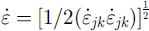. Constants in all simulations reported herein are n = 3, B = 0.2 MPa a^1/n (appropriate for temperatures at the pressure-melting point), ρ = 900 kg m⁻³, and g = −g ₂ = 9.8 m s⁻².

Equations (4) and (5) are solved on a finite-element grid consisting of four-node Taig quadrilaterals (Reference Irons and AhmadIrons and Ahmad, 1980). Velocity components are defined at each nodal point, whereas stresses, pressures and densities are constant across the element. The numerical equations are constructed using Galerkin’s method and two-point Gauss–Le-gendre integrals, producing a sparse, banded-symmetric set of linear equations that are solved via Gaussian elimination.

Grids for these models were constructed of elements in columns that were 5 m wide everywhere. Elements were 5 m high at the calving face, but increased back from the calving face in order to span the increasing glacier thickness without increasing the number of elements in a column. All of the grids for these experiments had perfectly flat bottoms, a calving face thickness, h ₀, of 100, 150, 200, 250 or 300 m, and a simulated length up-glacier from the calving face, L, of 2000 m. Only the section within a few hundred meters of the calving face was analyzed; the rest of the simulation was primarily intended to buffer the calving face from effects of the up-glacier boundary conditions.

In all our simulations, the internal dynamics of the ice were considered to be known. Thus, the changes we discuss arise solely from choices of boundary conditions. For a given set of boundary conditions, we normally made runs with the five values of h ₀ noted above.

Boundary conditions

In all simulations, the upper surface of the glacier and the subaerial part of the calving face were assumed to be stress-free.

Heights of subaerial parts of calving faces, h _c, are remarkably uniform. In ten of Reference Brown, Meier and PostBrown and others’ (1982) seventeen examples they are in the range 50–70 m, and in four others the uncertainties in the estimated heights allow the possibility of their being in this range. Consequently, in the modeling discussed herein we held h _c constant at 60 m and allowed the total height of the face, and hence water depth, to vary.

At the up-glacier boundary of the model domain, a horizontal velocity was specified in order to create an inflow of ice to the domain. In most simulations, this in flow was calculated from the Reference NyeNye (1952) plane-strain relation in which u(L, z) is determined by the surface slope and ice thickness, thus:

(7)

where α(L) and h(L) are the surface slope and ice thickness at the up-glacier end of the domain, and u _b(L) is the sliding velocity there, normally taken to be 1000 m a⁻¹.

The submarine part of the calving face had an applied stress boundary condition to account for the hydrostatic water pressure

(8)

where ρ _w is the density of sea water, 1030 kg m⁻³, and h _w is the water depth at the calving face.

Boundary conditions at the base of the simulated domain were more complicated. There, a mixed velocity and stress boundary condition was applied. The vertical component of the velocity was held fixed at w = 0. Horizontal velocities were free, but subjected to a resistive stress. The resistive stress, τ _b, was derived from consideration of force balances on the set of calving glaciers studied by Reference Brown, Meier and PostBrown and others (1982). Consider a section of a glacier of length X and width W in a rectangular channel. The thickness at the calving face is h ₀. Define a mean slope over the distance X such that . Balancing forces on this block yields the traction, τ _b, thus:

(9)

(e.g. Reference ThomasThomas, 1973), where is the longitudinal stress deviator at the upflow end of the block, is the mean thickness of the block, τ _s is the mean drag on fjord walls and A is a shape factor that accommodates convergence or divergence of the valley walls in the down-glacier direction (A = 1 if W is constant).

Let us now define another shape factor, S _f, to partition the drag forces between the bed and the fjord walls. Let . Thus, S _f = 0.5 corresponds to the situation in which half of the drag is supplied by the walls and half by the bed, whereas lower values of S _f represent situations in which less of the resistive stress is supplied by the bed, as might occur when basal water pressures are high. We now define a pressure-gradient forcing term, T:

(10)

Combining Equations (9) and (10) yields:

(11)

Values of T can now be calculated for the glaciers studied by Reference Brown, Meier and PostBrown and others (1982), using ice thicknesses and water depths at the calving face from their report, obtaining surface slopes from maps, assuming a horizontal bed and taking X = 1000 m. The values thus obtained were well correlated with h ₀ (Fig. 2a); a regression line of the form T = a + bh ₀ yielded a = 81 kPa and b = 0.667 kPa m⁻¹. If we assume that the driving stress over the block, τ _d, is constant and equal to pghα, the surface profile will be parabolic and described by:

(12)

where α ₀ is the surface slope at the calving face. Solving Equation (12) for α ₀ and combining the result with Equation (11), using T = a + bh ₀, provides a relation for the slope at the margin:

(13)

Figure 2b shows the resulting surface profiles for the standard set of ice thicknesses used in the simulations.

Fig. 2.

(a) Relation between T (Equation (11) ) and ice thickness at the calving face for glaciers studied by Reference Brown, Meier and PostBrown and others (1982). (b) Longitudinal surface profiles for standard set of ice thicknesses.

We used S _f T as an initial basal-stress boundary condition. (Shape factors are introduced in the model through modification of the value of B in Equation (6).) Use of S _f T as a stress boundary condition actually incorrectly transfers the force from the vertically integrated longitudinal stress deviator to the bed. As the model must iteratively solve the equations of motion, owing to the non-linear flow law, this problem was readily remedied by adjusting the basal-stress boundary condition during each iteration. In each iteration, the model estimates a velocity field, uses the velocities to calculate a strain-rate tensor field, uses those strain rates to reestimate the effective viscosity and then repeats the estimation of the velocity. The longitudinal stress field is generated essentially as a by-product of each model iteration, so the integrated longitudinal stress deviator could be subtracted from the basal boundary condition at each iteration. This did not appreciably increase the number of iterations required for model convergence, because the integrated longitudinal stress deviator is small compared to τ _b. In fact, it would not have changed our results significantly had we neglected this stress adjustment entirely.

Simulations with varying thickness

Some results of our modelling are presented in Figures 3–7. A pervasive feature is a zone of high u _i just below the waterline (Figs 3 and 4). Such a high speed might be anticipated from Hughes’ (Reference Hughes1992, fig. 3) analysis. As a result of this flow, there is a zone of very slight compression at the surface, extending about 50 m up-glacier from the calving face. This zone was present even in simulations, described below, that included crevasses.

Fig. 3.

Contours of horizontal velocity, u _i , in the last 500 m of a glacier 200 m thick at the calving face. S _f = 0.5 for this simulation. Contour interval is 5 m a⁻¹.

Fig. 4.

Variation with depth of horizontal velocity at the calving face for five different values of h₀ and two different values of S _f . Value of h₀ appropriate for any curve can be inferred from ordinate value of bottom of curve.

Fig. 5.

Variation in rate of overhang development with h₀ for S _f = 0.25 and 0.5. Lines are based on linear regressions.

Fig. 6.

Contours of in the last 500 m of a glacier that is 200 m thick at the calving face. Contour interval is 20 kPa. (a) S _f = 0.5. (b) S _f = 0.25.

Fig. 7

Longitudinal deviatoric stresses at the calving face and 20, 40, 60 and 80 m back from the calving face for (a) S _f = 0.5, h₀ = 100 m; (b) S _f = 0.5, h₀ = 200 m; (c) S _f = 0.5, h₀ = 300 m; and (d) S _f = 0.25, h₀ = 200 m.

In Figure 4 it will be seen that both u _i and the velocity gradient between the level of the velocity maximum and the bed increase with water depth, as one would expect. This velocity gradient is plotted as a function of h ₀ in Figure 5 for two different values of S _f. These velocity gradients are significant because they suggest that the calving face will tend to develop an overhang, and that this tendency will be greater on thicker glaciers. Such overhangs would promote failure (or collapse) of the top of a calving face, particularly one that was pervasively fractured.

Such oversteepenings are rarely noted, presumably because the ice collapses as fast as the overhang develops, and perhaps because the overhang is largely below sea level. For example, Reference Kirkbride and WarrenKirkbride and Warren (1997) say that they saw no evidence of gradual flow-induced overhang development in a sequence of photographs of the calving face of Maud Glacier, New Zealand. However, their photograph and sketches suggest that outward-leaning calving faces were present on occasion. Similarly, Reference MotykaMotyka (1997) reports that the calving face of LeConte Glacier, Alaska, has been observed to “lean outward … at various times”.

In Figures 6 and 7 we show some spatial variations in the longitudinal stress deviator, . There is a persistent high in Just below the water surface and a few tens of meters back from the calving face. Note that typically exceeds 100 kPa. Reference Van der VeenVan der Veen (1998b, p.41) notes that stresses of only about 30–80 kPa are needed for crevassing. Thus, the extensive crevassing observed up-glacier from the terminus of a calving glacier is readily understood.

There is a zone of high extending stresses along the bed near the calving face (Fig. 7). We attribute these stresses to the high vertical stresses needed to balance the bending moment applied to the terminus of the glacier by the unequal distribution of hydrostatic and cryostatic pressure on either side of the calving face (see also Reference ReehReeh, 1968; Reference HughesHughes, 1992, fig. 4). Such stresses would lead to a tendency toward extrusion flow near the base of the calving face, much as a column of ice sitting on a rigid substrate would tend to bulge out at the base. This would be likely to generate bottom crevasses. Reference Van der VeenVan der Veen (1998a) estimates that 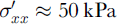is required to initiate bottom crevasses, and the stresses in Figure 7 are significantly larger than this. Such crevasses would promote submarine calving. Of particular interest is the fact that the average value of within 20 m of the calving face increases with water depth (Fig. 8). This could be another cause of an increase in u _c with increasing h _w.

Fig. 8.

Variation with h ₀ of mean at the bed within 20 m of the calving face.

Sensitivity studies

Some of the boundary conditions and modeling assumptions used in these simulations may be questioned. However, we found that the main conclusions are robust under a variety of different modeling scenarios. In what follows, we treat the run in which h ₀ = 200 m and S _f = 0.5 as a control experiment and test the effects of changing some of the boundary-condition parameters from those in the control run.

The overall length of the simulated domain, L, and the basal inflow into the up-glacier end of the domain, u _b(L), both affected the overall speed of the ice near the calving face without affecting the stresses. Simulations with u _b = 0 or 2000 m a⁻¹ at this face, compared with our standard u _b = 1000 m a⁻¹, simply added or subtracted 1000 m a⁻¹ from the velocities near the calving face. Increasing the overall length of the domain to 3000 or 4000 m showed that speeds increased as length increased. This demonstrates that we do not have a comprehensive simulation of the stress going well back from the calving face; rather, it seems likely that both basal and side drag increase up-glacier. However, neither the perturbations in u _b(L) nor those in L produced graphically visible changes in the longitudinal stress deviators or in shear stresses near the calving face.

Varying the water level for a constant glacier thickness (thus varying the height of the subaerial cliff) had a substantial effect on glacier speed, as would be expected: lower water levels decrease the back stress at the calving face, so the glacier moves faster. None of the results discussed here, however, were affected, as maxima in both speed and stress still appeared in the same positions relative to the waterline.

Crevasses provided a more interesting change in the results. A realistic depiction of downward-propagating surface cracks, the width of which varies with depth, and the depth of which varies almost at random, is beyond the scope and capability of the model. However, a characteristic of a glacier surface that is heavily crevassed into a serac field is that stresses are much more readily relieved by slippage along crevasse faces than in uncracked ice. We can thus simulate some aspects of the heavily crevassed surface by softening the ice, by means of a substantial decrease in B where B is understood to apply to the bulk, heavily cracked ice rather than to small-scale samples. Realistically, such an effect should be anisotropic, as there are preferred directions for stress relief, but that is also beyond reasonable use of a two-dimensional vertical model. The simulation also retains absolute mass conservation and incompressibility, which does not necessarily apply to an ice mass that is increasing its volume via crevassing.

In two perturbation runs, B was reduced by approximately a factor of 5, resulting in a 100-fold increase in for a given τ_jk , in elements in every third column within 500 m of the calving face. Thus, columns of softened ice 5 m wide were separated by columns of regular ice 10 m wide. In the two runs, the top four and eight elements, respectively, were thus softened, so these “crevasses” extended to depths of 20 and 40 m, respectively, at the margin. The depth increased slightly up-glacier as ice thickness increased.

One visible effect of crevassing is that it increases the overall speed of the glacier, top to bottom, and that greater depths of crevassing produce a greater speed increase (Fig. 9a). This may be true for a real glacier, but it should probably be considered a side-effect of the model. Softening some 3000–6000 m² of the flow plane is bound to cause a speed increase: the softening is numerically equivalent to reducing the side drag. The extension of the speed increase to the glacier bed indicates that even for a change applied only to the top 20 m, the 500 m of horizontal extent of change is sufficient to produce a response that is coupled 200 m downward to the bed.

Fig. 9.

Effects of crevasses on simulated speeds (a) and simulated longitudinal stress deviators (b) in a glacier 200 m thick.

The more interesting element of the speed increase is that its maximum is at the base of the crevassed zone, which enhances the velocity maximum at the waterline. Longitudinal stress deviators in the crevassed cases clearly show a decreased ice strength in the upper layers where softening has occurred, and a greater extension at the waterline (Fig. 9b). We conclude from both the horizontal velocity changes and the longitudinal stress deviator changes that effective softening of heavily crevassed near-surface ice increases the likelihood of buckling outward at the waterline, and hence enhances the effects seen in the uncrevassed case.

Conclusions

Calving speed increases with water depth, other factors remaining constant (Reference Brown, Meier and PostBrown and others, 1982; Reference Funk and RöthlisbergerFunk and Röthlisberger, 1989; Reference Pelto and WarrenPelto and Warren, 1991). If it turns out that there is a physical connection between u _c and h _w, despite Van der Veen”s (Reference Van der Veen1996, Reference Van der Veen1997) reservations, our modeling suggests that this may be, in part, because the distribution of longitudinal stresses and velocities leads to oversteepening of calving faces, with the rate of development of the oversteepening increasing with water depth. When the ice is pervasively fractured, as it must be when is so high, such oversteepening will destabilize the face, facilitating calving. In addition, zones of high at the base of the glacier near the calving face may promote bottom crevassing, particularly in thicker glaciers.

Calving rates are also known to increase in the fall (Reference SikoniaSikonia, 1982; Reference Meier, Rasmussen, Krimmel, Olsen and FrankMeier and others, 1985). This may also be partly due to oversteepening resulting from increased basal drag as subglacial water pressures decrease. In addition, the observation that calving speeds are highest when mean water temperatures are highest suggests that increased submarine melting, which would also lead to oversteepening, may play a role.

We think that this model of calving is consistent with both the Reference Brown, Meier and PostBrown and others (1982) and the Reference SikoniaSikonia (1982) calving relations. As noted, in an annual time-frame Brown and others found that calving rates increased linearly with water depth, and we find that the velocity field in the tongue of a calving glacier results in tendencies toward oversteepening and bottom crevassing that also increase with water depth; in the case of oversteepening, the increase is linear. Similarly, Sikonia inferred that on seasonal and sub-seasonal time-scales u _c varies directly with subglacial water discharge and inversely with effective pressure. By reducing basal drag, both of these may increase the speed at the base of the calving face (see effect of S _f in Fig. 4), thus facilitating failure by propagation of bottom crevasses.

In conclusion, we underscore the point made above (Equations (2–3)), that in certain situations, it may be a change in one of the variables, x _i, that results in a change in u _c, while in other situations it is another. Water depth is likely to be only one of the variables that affect calving speed.