
1. Introduction
Decomposition of the driving fluid force has been widely performed to gain insight into the mechanisms governing fluid–structure interaction in flow-induced vibration (FIV). For a bluff body with a single degree of freedom to vibrate in the cross-flow or streamwise direction, the fluid force is often decomposed into potential (inviscid) and vortical (viscous) components. The potential component is related to the ‘added mass’ arising from acceleration of surrounding fluid during the acceleration of a body in an inviscid irrotational fluid, and thus it is often referred to as the potential force or the added-mass force (see Limacher, Morton & Wood Reference Limacher, Morton and Wood2018). The vortical component is related to forcing associated with the surrounding time-varying vorticity field, noting that in general a flow field can be constructed from irrotational (potential) and rotational components (Lighthill Reference Lighthill1986; Govardhan & Williamson Reference Govardhan and Williamson2000; Limacher et al. Reference Limacher, Morton and Wood2018; Limacher Reference Limacher2021). This simple force decomposition approach has been useful in characterising FIV response regimes and transitions, and vortex-shedding modes, of bluff bodies vibrating transversely to a free stream (e.g. Govardhan & Williamson Reference Govardhan and Williamson2000; Zhao et al. Reference Zhao, Leontini, Lo Jacono and Sheridan2014; Soti et al. Reference Soti, Zhao, Thompson, Sheridan and Bhardwaj2018; Zhao, Hourigan & Thompson Reference Zhao, Hourigan and Thompson2018a, Reference Zhao, Hourigan and Thompson2019). However, for a body vibrating in-line, the make-up of the vortex force is more complex and it is useful to split the vortex force into different components to aid in developing a model representative of the flow physics. As demonstrated by Konstantinidis & Bouris (Reference Konstantinidis and Bouris2017), a decomposition of the vortex force based on Morison's equation (Morison, Johnson & Schaaf Reference Morison, Johnson and Schaaf1950) was only partially able to reconstruct the fluid force acting on a cylinder in non-zero-mean displacement oscillatory flows. Thus, building on previous studies, a key interest of the present study is to extend this force decomposition model for a cylinder freely vibrating in line with the free stream.
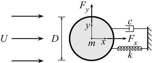
Figure 1 shows a schematic for the problem of interest: an elastically mounted cylinder is free to oscillate only in the streamwise direction, and the fluid–structure system is modelled as a single-degree-of-freedom mass-spring-damper oscillator subjected to a fluid flow. Key problem parameters are also defined in this figure. The body dynamics is governed by the linear second-order equation for a mass-spring-damper system:
 \begin{equation} m \ddot{x}(t) + c \dot{x}(t) + k x(t) = {{F_{x}}}(t) {,} \end{equation}
where  $m$ is the total oscillating mass of the system,
 $c$ is the structural damping of the system,
 $k$ is the spring constant,
 $x(t)$ is the body displacement and
 ${{F_{x}}}(t)$ represents the time-dependent (streamwise) fluid force acting on the cylinder. Note that the streamwise and transverse fluid force coefficients used in this study are defined by
 ${{{C_{x}}}} = {{F_{x}}} /((\rho U^2 D L)/{2})$ and
 ${{{C_{y}}}} = {{F_{y}}} /((\rho U^2 D L)/{2})$, respectively, where
 $\rho$ is the fluid density and
 $L$ is the cylinder immersed span. Often, the structural dynamics is characterised as a function of flow reduced velocity,
 ${U^*} = U/({{f_{{nw}}}} D)$, where
 ${{f_{{nw}}}}$ is the natural frequency of the system in quiescent fluid (i.e. water in the present study).
Problem set-up for in-line vortex-induced vibration of a circular cylinder showing key parameters.

Previous studies have focused on characterising the in-line VIV amplitude and frequency responses (e.g. Aguirre Reference Aguirre1977; Okajima et al. Reference Okajima, Nakamura, Kosugi, Uchida and Tamaki2004) and wake modes (e.g. Cagney & Balabani Reference Cagney and Balabani2013a,Reference Cagney and Balabanib; Konstantinidis Reference Konstantinidis2014). It has been shown widely in experimental studies that there generally exist two amplitude response branches in moderate- or high-Reynolds-number flows, while no branching behaviour has been observed in low-Reynolds-number numerical simulations (e.g. Bourguet & Lo Jacono Reference Bourguet and Lo Jacono2015; Konstantinidis, Dorogi & Baranyi Reference Konstantinidis, Dorogi and Baranyi2021). Note that the Reynolds number here is defined by  $\textit {Re} = UD/\nu$, with
 $\nu$ the kinematic viscosity of the fluid. Gurian, Currier & Modarres-Sadeghi (Reference Gurian, Currier and Modarres-Sadeghi2019) conducted experimental measurements of the streamwise fluid force, but without further decomposition analysis. Very recently, Konstantinidis et al. (Reference Konstantinidis, Dorogi and Baranyi2021) presented a force decomposition to shed light on the wake drag as the underlying driving component; however, when applied to our experimental data, their equations require modification. Therefore, there is still a need to develop an improved fluid forcing decomposition model that is consistent with the underlying force components in in-line VIV. This is particularly the case at moderate Reynolds numbers where the amplitude response is distinctly different from previous low-
 $\textit {Re}$ low-amplitude numerical studies. Thus, the primary contribution of the present work is to present this force decomposition extension, based on the model of Konstantinidis et al. (Reference Konstantinidis, Dorogi and Baranyi2021), to provide further insight into the dynamics in in-line VIV.
2. Experimental methodology
In the present study, the hydro-elastic system was modelled using a low-friction air-bearing rig in conjunction with a recirculating free-surface water channel of the Fluids Laboratory for Aeronautical and Industrial Research (FLAIR) at Monash University. Details of the air-bearing system and water-channel facilities have been described in the previous related studies of Zhao et al. (Reference Zhao, Hourigan and Thompson2018a,Reference Zhao, Lo Jacono, Sheridan, Hourigan and Thompsonb) and Wong et al. (Reference Wong, Zhao, Lo Jacono, Thompson and Sheridan2018).
The test cylinder model, precision-made from aluminium tubing, had an outer diameter of  $D = 40\pm 0.01\ {\rm mm}$. The immersed length of cylinder was
 $L = {614}\ {\rm mm}$, yielding a span-to-diameter aspect ratio of
 $AR = L/D = 15.4$. To reduce end effects of the cylinder and to promote parallel vortex shedding, an end conditioning platform was used (for more details, see Zhao et al. Reference Zhao, Hourigan and Thompson2018a,Reference Zhao, Lo Jacono, Sheridan, Hourigan and Thompsonb). The total oscillating mass of the system was
 $m = {1140.1}\ {\rm g}$, and the displaced mass of water was
 ${{m_{d}}} = \rho {\rm \pi}D^2 L/4 = {770.7}\, {\rm g}$, giving a mass ratio
 ${{m^{*}}} = m/m_{d} = 1.48$. The natural frequency of the mass-spring-damper system, determined via free decay tests, was found to be
 ${{f_{{na}}}} = {0.951}\ {\rm Hz}$ in air and
 ${{f_{{nw}}}} = {0.723}\ {\rm Hz}$ in quiescent water. Note that the structural damping ratio with consideration of the added mass was given by
 $\zeta = c / (2 \sqrt {k (m + {{m_{A}}})}) = 1.98\times 10^{-3}$, where the added mass, given by
 ${{m_{A}}} = (({{f_{{na}}}}/{{f_{{nw}}}})^2 -1) m$, was found to be 829.8 g. This equates to an experimentally defined added-mass coefficient, defined by
 ${{{C_{A}}}} = {{m_{A}}}/{{m_{d}}}$, of
 $1.08$, noting this is close to the theoretical potential added-mass coefficient of
 ${{{C_{A}}}}= 1$.
Measurement techniques for the cylinder vibration and fluid forces acting on the vibrating cylinder have been described and validated by Zhao et al. (Reference Zhao, Leontini, Lo Jacono and Sheridan2014, Reference Zhao, Hourigan and Thompson2018a,Reference Zhao, Lo Jacono, Sheridan, Hourigan and Thompsonb). The current VIV experiments were conducted over the reduced velocity range of  $1.40 \leqslant {U^*} \leqslant 5.00$ with fine increments of
 $0.05$, while the corresponding Reynolds number range was
 $1530 \leqslant \textit {Re} \leqslant 5450$. In addition, drag force measurements for a stationary cylinder over the same Reynolds number range were also conducted using a high-precision six-axis force sensor (Mini40, ATI-IA, US) with an accuracy of 5 mN (see Sareen et al. Reference Sareen, Zhao, Lo Jacono, Sheridan, Hourigan and Thompson2018).
The near wake of the cylinder was measured using the particle image velocimetry (PIV) technique. Details of the PIV system used can be found in Zhao et al. (Reference Zhao, Hourigan and Thompson2018a,Reference Zhao, Lo Jacono, Sheridan, Hourigan and Thompsonb). In the present experiments, in order to provide a thorough examination of changes of the near-wake flow structure, more than 100 000 images were obtained for 13 reduced velocities (9 are presented in the text of this paper, while the others are provided together as supplementary movies available at https://doi.org/10.1017/jfm.2022.359) across the VIV response regimes. The imaging was conducted at a sampling rate of 100 Hz for  $6200$ images in each dataset. To clearly visualise the evolution of the wake, images of each case were divided into
 $48$ phases per vortex-shedding cycle, giving each phase at least
 $100$ snapshots for averaging.
3. Results and discussion
3.1. Amplitude response and quasi-steady drag force
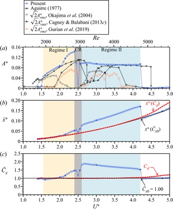
Figure 2 shows the normalised amplitude response ( ${A^{*}}$), the normalised time-averaged displacement (
 ${{\bar {x}^{*}}}$) of the cylinder from its neutral position at zero flow velocity, and the time-averaged streamwise fluid force coefficient (
 ${{{\bar{C}_{x}}}}$) as a function of reduced velocity. Note that in the present study the amplitude is represented by the mean of the top
 $10\,\%$ of amplitudes (
 ${{{A^{*}_{\rm{10}}}}}$, based on half of peak-to-peak values) at each
 ${U^*}$. As can be seen in figure 2(a), the present amplitude response can be characterised distinctly by two VIV regimes (namely regime I and regime II) and a competing regime (CR). In general, the two response regimes of the present work agree with those found in previous studies (for instance, see Aguirre (Reference Aguirre1977) with a similar mass ratio of
 $1.46$). However, discrepancies in some details may be attributable to differences in mass ratio, damping ratio and Reynolds number, but these aspects are beyond the focus of the present study.
The variation of  $(a)$ the normalised amplitude response,
 $(b)$ time-averaged displacement and
 $(c)$ time-averaged streamwise fluid force coefficient as a function of reduced velocity. In
 $(a)$, the vibration response regimes in the present study are shaded in different colours: VIV regime I in light yellow, CR in grey and VIV regime II in light blue. For Aguirre (Reference Aguirre1977),
 ${{m^{*}}} = 1.46$ (
 $\zeta$ unknown),
 $\textit {Re} = 1 \times 10^3\unicode{x2013}3\times 10^5$; for Okajima et al. (Reference Okajima, Nakamura, Kosugi, Uchida and Tamaki2004),
 ${{m^{*}}} \zeta = 0.49$ (
 ${{m^{*}}}$ and
 $\zeta$ individually unknown),
 $\textit {Re} = 8 \times 10^3\unicode{x2013}4\times 10^4$; for Cagney & Balabani (Reference Cagney and Balabani2013b),
 ${{m^{*}}} = 1.17$ and
 $\zeta \approx 5.3\times 10^{-3}$,
 $\textit {Re} = 450\unicode{x2013}3700$; and for Gurian et al. (Reference Gurian, Currier and Modarres-Sadeghi2019),
 ${{m^{*}}} = 1.61$ and
 $\zeta = 6\times 10^{-3}$,
 $\textit {Re} = 970\unicode{x2013}3370$. In
 $(b)$, the dotted line in red and the solid line in black represent the evaluations of
 ${{\bar {x}^{*}}}({{{C_{d}}}} )$ and
 ${{\bar {x}^{*}}}(\bar {C}_{x_0})$ by substituting
 ${{{C_{d}}}}$ and
 $\bar {C}_{x_0}$ for (3.1), respectively. In
 $(c)$, the dotted line in red represents the measurements of
 ${{{C_{d}}}}$, while the horizontal line in black represents
 $\bar {C}_{x_0}$. Note that the circles filled in blue represent spot PIV measurements.

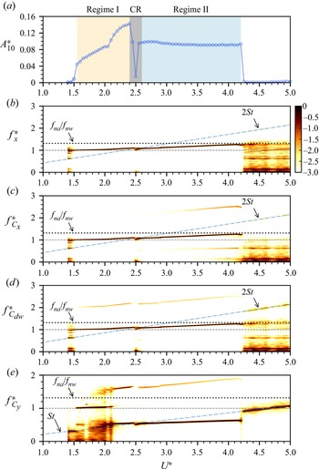
In regime I (covering the range  $1.55 \leqslant {U^*} \leqslant 2.40$), the vibration amplitude increases gradually to reach its peak value of
 ${{A^{*}_{\rm {10}}}} = 0.144$ as
 ${U^*}$ is increased to
 $2.40$. In this regime, the body vibration frequency (
 ${f^*_x}$) is synchronised with the fluid forcing frequency (
 ${f^*_{C_x}}$), as shown in figure 3(b,c). Note that the frequency components are normalised by the natural frequency of the system in quiescent water, namely
 ${f^{*}} = f/{{f_{{nw}}}}$. It is interesting to note that both
 ${f^*_x}$ and
 ${f^*_{C_x}}$ tend to increase slightly with
 ${U^*}$ beyond
 ${U^*} \simeq 2.1$. When both
 ${f^*_x}$ and
 ${f^*_{C_x}}$ approach the slope of
 $2{St}$ (
 $\text {Strouhal number} = {St} = Df/U = 0.215$ measured over the Reynolds number range tested), the amplitude response experiences an abrupt drop at
 ${U^*} = 2.45$ (
 ${\approx }1/(2{St})$), due to the competition between non-stationary (i.e. changing with time) frequency responses of the body vibration and the vortex shedding, noting that the streamwise fluid force generally exhibits a dominant frequency twice that of the cross-flow fluid force (
 ${f^*_{C_y}}$) for a fixed body. As shown in figure 2, the sudden drop of amplitude response in this regime has also been observed occurring over different
 ${U^*}$ ranges in the previous studies with different structural properties; however, no detailed investigations into this regime have yet been reported. More features of the CR will be further discussed later. As
 ${U^*}$ is increased slightly further to
 $2.60$, frequency synchronisation between the body vibration and driving fluid force is resumed in regime II for
 ${U^*}$ up to 4.20, where the vibration amplitude is found to be almost constant at
 ${{A^{*}_{\rm {10}}}} = 0.094$ throughout. Still, both
 ${f^*_x}$ and
 ${f^*_{C_x}}$ tend to increase slightly with
 ${U^*}$, until desynchronisation is encountered when they approach the natural frequency of the system in air (i.e.
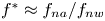 ${f^{*}} \approx {{f_{{na}}}}/{{f_{{nw}}}}$).
Normalised amplitude and logarithmic-scale power spectrum density contours of normalised frequency responses as a function of reduced velocity. Note that  $f^*_{C_{dw}}$ represents the normalised frequency of the wake drag.

To take the analyse further, we examine the time-averaged cylinder position and the time-averaged streamwise fluid force coefficient. Following the analytical approach used by Zhao et al. (Reference Zhao, Lo Jacono, Sheridan, Hourigan and Thompson2018b), by taking temporal averages of both sides of (1.1), the time-averaged cylinder displacement in dimensionless form (normalised by the cylinder diameter  $D$) can be expressed as
 \begin{equation} {{\bar{x}^{*}}} = \frac{{U^*}^2 {{{\bar{C}_{x}}}}}{2{\rm \pi}^3({{m^{*}}} + {{{C_{A}}}})}. \end{equation}
Interestingly, as shown in figure 2(b),  ${{\bar {x}^{*}}}$ deviates from the values of
 ${{\bar {x}^{*}}}({{{C_{d}}}} )$ and
 ${{\bar {x}^{*}}}(\bar {C}_{x_0})$, which are evaluated by substituting
 ${{{C_{d}}}}$ and
 $\bar {C}_{x_0}$, respectively, for
 ${{{\bar{C}_{x}}}}$ in (3.1), noting that
 ${{{C_{d}}}}$ is the quasi-steady drag coefficient measured for the fixed cylinder case, while
 $\bar {C}_{x_0}$ is the average of
 ${{{\bar{C}_{x}}}}$ taken for the desynchronised locations of insignificant vibration (i.e.
 ${U^*} > 4.2$). Similar deviations have been observed for in-line FIV of a rotating cylinder by Zhao et al. (Reference Zhao, Lo Jacono, Sheridan, Hourigan and Thompson2018b), when the cylinder experienced large-amplitude oscillations. It is also interesting to note in the present study that
 $\bar {C}_{x_0}$ deviates from
 ${{{C_{d}}}}$ for high reduced velocities (i.e.
 ${U^*} > 4.1$), which in turn leads to the differences between
 ${{\bar {x}^{*}}}({{{C_{d}}}} )$ and
 ${{\bar {x}^{*}}}(\bar {C}_{x_0})$. However, these significant deviations could not be explained by the previous force decomposition of Konstantinidis et al. (Reference Konstantinidis, Dorogi and Baranyi2021), as they were neglected in low-Reynolds-number flows (
 $Re = 100\unicode{x2013}250$). To better understand the underlying physics of the resonant response, we perform a decomposition analysis for the driving fluid force in the following § 3.2.
3.2. Decomposition of the driving fluid force
Assuming that the cylinder vibration in fluid–structure synchronisation can be represented by a single-frequency harmonic function of time, the cylinder displacement and the streamwise fluid force can be expressed by (3.2) and (3.3), respectively:
 $$\begin{gather} x(t) = \bar{x} + A \cos(\omega t) {,} \end{gather}$$
 $$\begin{gather}{{F_{x}}}(t) = {{\bar{F}_{x}}} + {{\tilde{F}_{x}}} \cos(\omega t + {{\phi_{x}}}) , \end{gather}$$
where  ${{\bar {F}_{x}}}$ and
 ${{\tilde {F}_{x}}}$ are the time-averaged component and the magnitude of the fluctuating component of
 ${{F_{x}}}$, respectively, while
 ${{\phi _{x}}}$ is the phase between
 ${{F_{x}}}$ and
 $x$ (also referred to as the total phase);
 $\omega = 2{\rm \pi} f$ is the angular frequency.
Following the force decomposition method proposed by Konstantinidis et al. (Reference Konstantinidis, Dorogi and Baranyi2021), who extended the equation of Morison et al. (Reference Morison, Johnson and Schaaf1950) to include a wake drag term, the streamwise fluid force is given as follows:
 \begin{equation} {{F_{x}}}(t) = \tfrac{1}{2}\rho D L {{{C_{d}}}} |U - \dot{x}|(U - \dot{x}) - {{m_{A}}} \ddot{x} + {{{F_{dw}}}} (t) {,} \end{equation}
where the first term represents the quasi-steady drag experienced by a fixed cylinder that is subjected to a relative flow speed  $(U - \dot {x})$, the second term represents the potential force (the inviscid added-mass force) associated with the body acceleration, and the third term represents the wake drag. In particular, different from Konstantinidis et al. (Reference Konstantinidis, Dorogi and Baranyi2021), we here further decompose the wake drag into a steady component and an unsteady component due to periodic vortex formation in the cylinder wake, given by
 \begin{equation} {{{F_{dw}}}} (t) = {{{\bar{F}_{dw}}}} + {{{\tilde{F}_{dw}}}} \cos(\omega t + {{\phi_{dw}}}) , \end{equation}
where  ${{{\bar{F}_{dw}}}}$ is the (time-averaged) steady component, while
 ${{{\tilde{F}_{dw}}}}$ is the magnitude of the unsteady component with a phase,
 ${{\phi _{dw}}}$, with respect to the body displacement
 $x$. By neglecting the terms involving second or higher orders of
 $\sin (\omega t)$ and
 $\cos (\omega t)$, the streamwise fluid force can be approximated as
 \begin{align} {{F_{x}}}(t) &= \frac{1}{2} \rho U^2 D L \left[{{{C_{d}}}} + \frac{2 \omega A}{U} \sin(\omega t) + {{{\bar{C}_{dw}}}} + {{{\tilde{C}_{dw}}}} \cos(\omega t + {{\phi_{dw}}}) \right] \nonumber\\ &\quad +\frac{1}{4} {\rm \pi}\rho D^2 L {{{C_{A}}}}\omega^2 A \cos(\omega t). \end{align}
The above equation indicates that the steady part of the streamwise fluid force consists of contributions from the quasi-steady drag ( ${{{C_{d}}}}$) and the steady component of the wake drag (
 ${{{\bar{C}_{dw}}}}$):
 \begin{equation} {{\bar{F}_{x}}} = \tfrac{1}{2} \rho U^2 D L \left({{{C_{d}}}}+ {{{\bar{C}_{dw}}}}\right), \end{equation}
or in dimensionless form
 \begin{equation} {{{\bar{C}_{x}}}} = {{{C_{d}}}}+ {{{\bar{C}_{dw}}}}. \end{equation}
Importantly, this expression reflects that the mean wake drag, in addition to the quasi-steady drag, can contribute to the steady component of the driving fluid force when the cylinder is given the degree of freedom to oscillate streamwise. This approach presents a significant modification of the original model of Konstantinidis et al. (Reference Konstantinidis, Dorogi and Baranyi2021) that gives  ${{{\bar{C}_{x}}}} = {{{C_{d}}}}$. Indeed in that model
 ${{{\bar{C}_{dw}}}}$ was not considered, and thus the deviations in both
 ${{\bar {x}^{*}}}$ and
 ${{{\bar {C}_{x}}}}$ curves during VIV could not to be explained, noting the significant departures shown in figure 2. To comment further, for the cases considered by Konstantinidis et al. (Reference Konstantinidis, Dorogi and Baranyi2021) of
 $\textit {Re}=100$ and 180, the peak oscillation amplitudes are so small that the movement of the cylinder during oscillation (
 ${\sim }1\,\%D$ or less) hardly causes any modification of the wake from that of a stationary cylinder. Hence in that case, there is hardly any change to the mean drag force whether the cylinder oscillates or not. On the other hand, for the higher Reynolds numbers considered here, the oscillation amplitude is larger, although still relatively small (
 ${\sim }10\,\%D$). However, this is enough to cause the motion of the cylinder to modify the wake and mean drag force to be noticeably different from those of a stationary cylinder.
The unsteady part of  ${{F_{x}}}$ can also be written in a dimensionless form:
 \begin{equation} {{{\tilde{C}_{x}}}} \cos(\omega t + {{\phi_{x}}}) = \frac{2 \omega A}{U} {{{C_{d}}}}\sin(\omega t) + {{{\tilde{C}_{dw}}}} \cos(\omega t + {{\phi_{dw}}}) + \frac{{\rm \pi} D \omega^2 A}{2 U^2} {{{C_{A}}}}\cos(\omega t). \end{equation}
By equating the cosine and sine terms expanded through the double-angle formulae for the above equation, we can find the following relationships:
 $$\begin{gather} {{{\tilde{C}_{dw}}}} \sin{{\phi_{dw}}} = {{{\tilde{C}_{x}}}} \sin{{\phi_{x}}} + \frac{2\omega A}{U} {{{C_{d}}}}= {{{\tilde{C}_{x}}}} \sin{{\phi_{x}}} + \frac{4 {\rm \pi}{f^{*}} {A^{*}}}{{U^*}} {{{C_{d}}}}, \end{gather}$$
 $$\begin{gather}{{{\tilde{C}_{dw}}}} \cos{{\phi_{dw}}} = {{{\tilde{C}_{x}}}} \cos{{\phi_{x}}} - \frac{{\rm \pi} D \omega^2 A}{2 U^2} {{{C_{A}}}}= {{{\tilde{C}_{x}}}} \cos{{\phi_{x}}} - 2{\rm \pi}^3 \left(\frac{{f^{*}}}{{U^*}}\right)^2 {A^{*}} {{{C_{A}}}}. \end{gather}$$
Substituting (3.2) and (3.3) for the governing equation of motion (1.1), with the natural frequency of the system in vacuum  $f_n$, we can obtain the following relationships:
 $$\begin{gather} {{{\tilde{C}_{x}}}} \sin{{\phi_{x}}} = \frac{4 {\rm \pi}^3 {f^{*}} {A^{*}}}{{U^*}^2} {{m^{*}}} \zeta \left(\frac{{{f_{n}}}}{{{f_{{nw}}}}}\right)^2 = \frac{4{\rm \pi}^3 {f^{*}} {A^{*}}}{{U^*}^2}({{m^{*}}} + {{{C_{A}}}}) \zeta , \end{gather}$$
 $$\begin{gather}{{{\tilde{C}_{x}}}} \cos{{\phi_{x}}} = \frac{2 {\rm \pi}^3{{m^{*}}} {A^{*}}}{{U^*}^2} \frac{({{f_{n}}}^2 - f^2 )}{{{f_{{nw}}}}^2} = \frac{2{\rm \pi}^3 {A^{*}}}{{U^*}^2} \left[{{m^{*}}}(1-{f^{*}}) + {{{C_{A}}}}\right]. \end{gather}$$
It should be noted that in addition to our new decomposition leading to (3.8), we have also obtained the modified expressions in (3.10)–(3.13) to those given by Konstantinidis et al. (Reference Konstantinidis, Dorogi and Baranyi2021). Furthermore, by substituting (3.12) for (3.10), the dimensionless vibration amplitude in steady state can be evaluated by
 \begin{equation} {A^{*}} = \frac{{U^*}^2 {{{\tilde{C}_{dw}}}} \sin{{\phi_{dw}}}}{4{\rm \pi} {f^{*}} \left[{\rm \pi}^2 ({{m^{*}}} + {{{C_{A}}}})\zeta + {U^*}{{{C_{d}}}}\right]} . \end{equation}
This expression indicates that the vibration amplitude depends on the unsteady component of the wake drag and its phase. Note that this is significantly different from that of Konstantinidis et al. (Reference Konstantinidis, Dorogi and Baranyi2021) (their (4.7)), which is much simplified and with the wake drag phase term missing, an important parameter to evaluate  ${A^{*}}$ in steady state. A direct comparison between the amplitude response predicted using (3.14) and experimental data is presented in § 3.4.
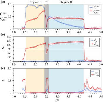
Through the decomposition of  ${{F_{x}}}$, we can determine the wake drag to gain a better understanding of the dynamics of the fluid–structure system. Figure 4 shows the root-mean-square coefficients of the streamwise fluid force and wake drag (
 ${{{C_{x}^{rms}}}}$ and
 ${{C_{{dw}}^{rms}}}$), together with their mean phases and phase variants (with respect to
 $x$), as a function of reduced velocity. The mean phase is obtained by projecting the phase differences between two signals onto the unit circle in a complex plane and calculating the mean resultant vector of the angular phase distribution, as given by
 \begin{equation} \bar{\boldsymbol{\varPhi}} = \frac{1}{N}\sum^{N}_{j=1}{\rm e}^{{\rm i}\phi_j}, \end{equation}
where  $\phi _j$ is the relative phase between the two signals at an instance and
 $N$ is the total number of samples of a signal (McQueen et al. Reference McQueen, Zhao, Sheridan and Thompson2021). Thus, the mean phase angle can be determined by
 \begin{equation} \bar{\phi} = \mathrm{Arg}(\bar{\boldsymbol{\varPhi}}), \end{equation}
and the mean phase coherence based on the circular variance of the phase distribution can be indicated by
 \begin{equation} \sigma = 1 - |\bar{\boldsymbol{\varPhi}}|, \end{equation}
where  $0 \leqslant \sigma \leqslant 1$ is used as the index of phase synchronisation. The minimum possible value,
 $0$, indicates that all phase angles are equal (i.e. perfect phase synchronisation), whereas the maximum,
 $1$, indicates that the phase angles are spread uniformly over the circular space (i.e. no phase synchronisation or uncorrelated phase differences).
Variations of the streamwise fluid force and wake drag coefficients, together with the mean phases (in degrees) and their variants, as a function of reduced velocity.

As can be seen in figure 4, the coefficients of fluid forces, and the mean phases and their synchronisation indices, experience changes corresponding to changes in the frequency responses in figure 3. Notably, both  ${{C_{y}^{rms}}}$ and
 ${{C_{{dw}}^{rms}}}$ display an abrupt jump at the onset of regime I, and then another deflection change at
 ${U^*} \approx 2.05$. Interestingly, the notable V-shape drop in
 ${{C_{y}^{rms}}}$ at
 ${U^*} \approx 2.05$ corresponds to a sharp change in the dominant component of
 ${f^*_{C_y}}$ shifting from
 ${f^*_{C_y}} = {f^*_x}$ to
 ${f^*_{C_y}} = 0.5{f^*_x}$ (figure 3e). After the abrupt drop in the CR,
 ${{{C_{x}^{rms}}}}$ and
 ${{C_{{dw}}^{rms}}}$ increase rapidly at the beginning of regime II. However, as it is expected from (3.13),
 ${{{C_{x}^{rms}}}}$ tends to decrease to minimal or zero, as the vibration frequency increases gradually towards
 ${{f_{{na}}}}$ at the end of regime II. Through the
 ${U^*}$ range tested,
 ${{F_{x}}}$ remains in phase with
 $x$, i.e.
 ${{\phi _{x}}} \simeq 0^\circ$. On the other hand, the variation of
 ${{C_{{dw}}^{rms}}}$ resembles that of
 ${A^{*}}$, which would be expected from (3.14). Interestingly, the wake drag phase
 ${{\bar {\phi }_{dw}}}$ undergoes a sudden jump to
 $91^\circ$ at the beginning of regime I and then increases to
 $130^\circ$ at the end of the regime. The change of the dominant frequency of
 ${f^*_{C_y}}$ and the variation of
 ${{\bar {\phi }_{dw}}}$ imply the existence of different wake patterns in this regime, as expected from previous studies. In regime II,
 ${{\bar {\phi }_{dw}}}$ is found to be stable at approximately
 $138^{\circ }$. Further discussion on wake modes is presented in § 3.3.
Moreover, the variants of the phases ( ${{\sigma _x}}$ and
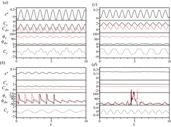
 ${{\sigma _{{dw}}}}$) in figure 4(c) show that the driving force components are in phase synchronisation with cylinder vibration in both regimes I and II. Interestingly, time traces of the wake drag force shown in figure 5(b) revealed that
 ${{\phi _{dw}}}$ sweeps through from
 $0^\circ$ to
 $360^\circ$, indicating a phase desynchronisation in the CR, which is distinctly different from regimes I and II (see
 ${U^*} = 2.40$ and
 $3.00$ in figures 5(a) and 5(c), respectively), where
 ${{\phi _{x}}}$ and
 ${{\phi _{dw}}}$ fluctuate slightly about their stable mean value; that is, the phase desynchronisation leads to a chaotic dynamical response in this regime.
Sample time traces of the cylinder displacement, fluid force coefficients and their phases (in degrees) at different reduced velocities:  $(a)$
 ${U^*} = 2.40$,
 $(b)$
 ${U^*} = 2.50$,
 $(c)$
 ${U^*} = 3.00$ and
 $(d)$
 ${U^*} = 4.80$. Note that
 ${{{C_{dw}}}}$ and
 ${{\phi _{dw}}}$ are denoted by the dashed lines. Note that
 $\tau$ is the normalised time given by
 $\tau = {{f_{{nw}}}} t$ to indicate body vibration cycles.

3.3. Time-frequency analysis and wake modes
To provide an insight into the dynamics of the cylinder vibration and the wake structure, this subsection presents a time-frequency analysis and PIV measurements undertaken at various reduced velocities across the VIV response regimes.
The time-frequency analysis is based on continuous wavelet transform (CWT), and the ‘mother’ wavelet used is a complex Morlet wavelet. In the present analysis, the centre frequency of the mother wavelet is set equal to  ${{f_{{nw}}}}$, while the bandwidth is set at
 $10/{{f_{{nw}}}}$ (approximately 10 cylinder vibration cycles) for cases in regimes I and II, where the cylinder vibration is highly periodic, and
 $3 /{{f_{{nw}}}}$ for cases in the CR and desynchronisation regime to better capture intermittent changes in the dynamic signals. This CWT method has been used by Nemes et al. (Reference Nemes, Zhao, Lo Jacono and Sheridan2012) and Zhao et al. (Reference Zhao, Nemes, Lo Jacono and Sheridan2018c) to reveal intermittent behaviour and branch competition of FIV responses for square cylinders.
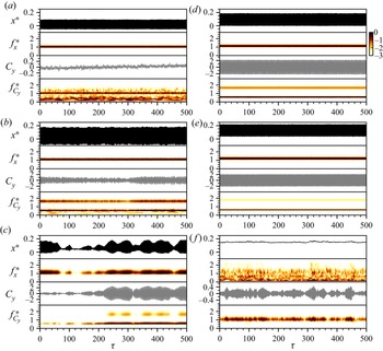
Figure 6 shows the time-frequency variations of the cylinder vibration and the transverse lift (coefficient), which reflects the vortex-shedding frequency, at  ${U^*} = [1.80, 2.35, 2.55, 2.80, 3.50, 4.80]$. Note that the measurements for each case in this figure were taken over 1200 s (more than
 $900$ vibration cycles) in order to reveal non-stationary frequencies and intermittent behaviour. Based on the transverse lift frequency response in figure 3(e), regime I can be further divided into two parts:
 $1.55 \leqslant {U^*} \lesssim 2.1$, where the dominant component of
 ${f^*_{C_y}}$ matches that of
 ${f^*_x}$, and
 $2.1 < {U^*} \leqslant 2.4$, where the dominant component of
 ${f^*_{C_y}}$ appears at
 $0.5{f^*_x}$, accompanied by a harmonic at
 $1.5{f^*_x}$. This change in the dominant frequency of
 ${f^*_{C_y}}$ implies a corresponding change in wake mode. As shown in figure 6(a), at
 ${U^*} = 1.80$ selected from the middle of first part of regime I, the cylinder vibration is highly periodic with its dominant frequency as stationary (i.e. not changing with time) slightly above
 ${{f_{{nw}}}}$, while
 ${f^*_{C_y}}$ also displays its stationary dominant component matching
 ${f^*_x}$, but accompanied by a non-stationary subharmoic (
 ${\sim }0.5{f^*_x}$) with relatively strong power varying with time. As expected, the phase-averaged PIV results of
 ${U^*} = 1.60$ and
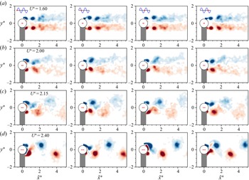
 $2.00$ in figures 7(a) and 7(b), respectively, show a symmetric vortex-shedding mode, where a pair of opposite-sign vortices are shed simultaneously from both sides of the cylinder. This symmetric wake pattern agrees with the symmetric ‘S-I’ mode reported in the previous studies of Cagney & Balabani (Reference Cagney and Balabani2013a,Reference Cagney and Balabanib), Okajima et al. (Reference Okajima, Nakamura, Kosugi, Uchida and Tamaki2004), and Gurian et al. (Reference Gurian, Currier and Modarres-Sadeghi2019). Unsurprisingly, in the present experiments, the symmetry of this wake mode is associated with very low lift coefficient magnitudes (figure 6a), due to the simultaneously symmetric wake structure and, thus so, the pressure distribution around the cylinder. However, it is worth noting that the vortices of this symmetric mode tend to break up towards the cylinder's equilibrium position as
 ${U^*}$ is increased in this subregime, e.g. the breakdown of vortices occurs at
 ${{\tilde {x}^{*}}} \approx 2.5$ for
 $U^* = 1.60$, and at
 ${{\tilde {x}^{*}}} \approx 1.5$ for
 $U^* = 2.00$. Further increasing
 ${U^*}$ will cause the breakdown of vortices to occur close to the cylinder body, thus leading to a change of the wake mode in the second subregime.
Continuous-wavelet-transform-based time-frequency analysis for the body vibration and the transverse lift coefficient at different reduced velocities selected from the VIV response regimes. For convenience of comparison, the left column plots two cases  ${U^*} = 1.8$ and
 $2.35$ from regime I and one case
 ${U^*} = 2.55$ from CR in (a–c), respectively, while the right column presents two cases
 ${U^*} = 2.8$ and
 $3.5$ from regime II and one case
 ${U^*} = 4.8$ from desynchronisation regime in (e–f), respectively.

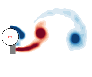
Phase-averaged vorticity contours (of selected phases) showing the evolution of the wake patterns for various reduced velocities across regime I:  ${U^*} \in [1.60, 2.00, 2.15, 2.40]$ in (a–d), respectively. The normalised vorticity range shown here is
 $\omega ^*_z = [-5, 5]$. The horizontal bar in red placed at the cylinder centre represents the peak-to-peak vibration amplitude. The red dots on the sine waves in (a) denote the cylinder position during its vibration. For the full oscillation cycles, see supplementary movie 1 for all test cases in regime I.

Indeed, the second part of regime I sees a different wake mode comprising two single opposite-sign vortices shed simultaneously but alternating in size from both sides of the cylinder per shedding cycle (or per two cylinder vibration cycles). This wake mode is termed ‘AS’ (alternating-symmetric) mode by Gurian et al. (Reference Gurian, Currier and Modarres-Sadeghi2019). Correspondingly, as previously mentioned,  ${f^*_{C_y}}$ exhibits a different composition with its dominant component at
 $0.5{f^*_x}$ and a harmonic at
 $1.5{f^*_x}$ (figure 3e), while the CWT result in figure 6(b) indicates that these frequency components remain almost constant in power over time. On the other hand, the phase-averaged vorticity fields in figure 7(c) show that vortices tend to become stronger as
 ${U^*}$ is increased; that is, at
 ${U^*} = 2.15$ (and
 $2.25$ and
 $2.30$ in supplementary movie 1) the vortices seem to dissipate significantly as they travel downstream, while at the high-end reduced velocity
 ${U^*} = 2.40$, the vortices remain clearly in a strong AS pattern travelling through the measurement field of view. As expected, this mode causes significant fluctuating lateral fluid forces acting on the cylinder. Notably, these strong vortices induce an amplitude peak significantly greater than those reported in previous studies (as compared in figure 2).
Interestingly, as  ${U^*}$ is further increased in the CR, both
 ${f^*_x}$ and
 ${f^*_{C_y}}$ exhibit intermittent behaviour. This is demonstrated by the case of
 ${U^*} = 2.55$ in figure 6(c), where significant cylinder oscillations (i.e. with
 ${A^{*}} \approx 0.1$) accompanied with well-defined harmonics of
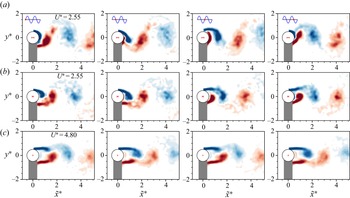
 ${f^*_{C_y}}$ are encountered intermittently in an unpredictable way. Such a chaotic response is similar to the branch competing behaviour in FIV of inclined square cylinders reported by Nemes et al. (Reference Nemes, Zhao, Lo Jacono and Sheridan2012) and Zhao et al. (Reference Zhao, Nemes, Lo Jacono and Sheridan2018c). On the other hand, however, as shown in figure 8(a,b), the wake measurements taken separately for large- and low-amplitude oscillation cycles show similar patterns, while the vortices associated with large-amplitude cycles seem to be slightly stronger. When compared with the desynchronisation case of
 ${U^*} = 4.80$ in figure 8(c), despite similar (Kármán-like) patterns observed further downstream (
 ${{\tilde {x}^{*}}} > 2$), the CR cases see strong shear-layer wrapping across the centreline of the cylinder wake. Nevertheless, the vortices in the CR do not seem to have well-defined regular shapes as in regimes I and II, thus seem less able to maintain consistent forcing responsible for the cylinder vibration.
Phase-averaged vorticity contours (of selected phases) showing the evolution of the wake patterns at  ${U^*} = 2.55$ in the CR and
 ${U^*} = 4.80$ in the desynchronisation regime. Note that
 $(a)$ presents the PIV measurements taken for large-amplitude oscillation cycles (i.e.
 ${A^{*}} \approx 0.1$) at
 ${U^*} = 2.55$, and
 $(b)$ for low-amplitude oscillation cycles (i.e.
 ${A^{*}} \lesssim 0.03$) . For more details, refer to the caption of figure 7. For the full oscillation cycles, see supplementary movie 2.

When  ${U^*}$ is further increased into regime II, highly periodic vibration resumes. As shown in figures 6(d) and 6(e) for two cases
 ${U^*} = 3.00$ and
 $4.20$,
 ${f^*_x}$ remains stationary over time, while
 ${f^*_{C_y}}$ also remains stationary but its harmonic component at
 $1.5{f^*_x}$ tends to become weaker as
 ${U^*}$ is increased. On the other hand, the wake patterns in figure 9 show similar major structures, which are in agreement with previous studies (i.e. the A-IV mode reported by Cagney & Balabani Reference Cagney and Balabani2013b). The present study, for the first time, extends wake measurement beyond
 ${U^*} = 4.0$ for regime II. It is interesting to note that the elongated shear layers tend to become stronger with increasing
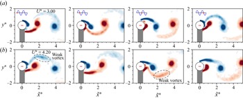
 $U^*$ in this regime, and at high reduced velocities they can form a secondary weak vortex each time a major vortex sheds, making the wake pattern appear as a
 ${P_{{o}}}$ mode (namely, a pair of vortices consisting of a strong vortex and a relatively much weaker one in each pair shed per cycle) – see supplementary movie 3 for animations of full vortex-shedding cycles. With multiple vortices shed per cycle, this
 $P_{{o}}$ mode should explain why the harmonic component of the drag force frequency
 ${f^*_{C_x}}$ appears and tends to become stronger with increasing
 ${U^*}$ in regime II (figure 3c).
Phase-averaged vorticity contours (of selected phases) showing the evolution of the wake patterns at  ${U^*} = 3.00$ and
 $4.20$ in regime II. For more details, refer to the caption of figure 7. For the full oscillation cycles, see supplementary movie 3 for all test cases in regime II.

3.4. Evaluation of amplitude response based on wake drag
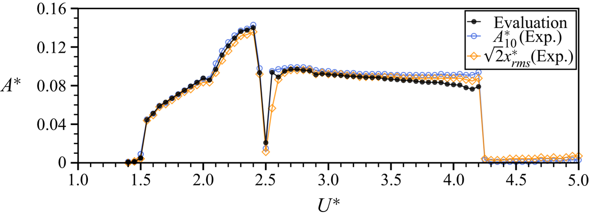
In order to validate our force decomposition analysis, we evaluate the vibration amplitude based on (3.14) and compare it with the experimentally measured response in figure 10. As shown, the evaluated amplitude response closely matches the actual values of  ${{A^{*}_{\rm {10}}}}$ and
 $\sqrt {2} A^*_{rms}$ (or
 $\sqrt {2}x^*_{rms}$) for most of the
 ${U^*}$ range tested. Subtle differences observed for
 $3.5 \lesssim {U^*} \leqslant 4.2$ in regime II could be attributable to the fact that the power of the harmonic components in
 ${f^*_{C_x}}$ (figure 3c) tends to increase in this
 ${U^*}$ range (still of two orders weaker than the dominant frequency), affecting the evaluation based on harmonic approximations. (In the present experiment, we did not extend the evaluation to the desynchronisation regime beyond
 ${U^*} = 4.2$, where the harmonic assumption is not applicable). Nevertheless, the above results have validated the force decomposition and the harmonic approximations.
Evaluation of amplitude response as a function of reduced velocity.

4. Conclusions
Decomposition has been performed for the driving fluid force on an elastically mounted circular cylinder undergoing in-line vortex-induced vibration in a free-stream flow. Based on the carefully conducted experiments, we have updated the wake drag model proposed previously by Konstantinidis et al. (Reference Konstantinidis, Dorogi and Baranyi2021) to include a steady and an unsteady part. This approach reflects that, when the cylinder is allowed to oscillate streamwise, the oscillation alters the time-dependent wake in turn altering the time-averaged displacement of the cylinder as well as the time-averaged streamwise fluid force from those experienced without cylinder oscillation. A harmonic approximation analysis was adopted to derive the relationship between the total streamwise fluid force and the wake drag. This analysis has been validated by predicting the amplitude response to directly compare with experimental measurements, meaning that prediction of amplitude response based on the updated wake drag model would be possible for various conditions of flow velocity and structural properties.
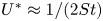
The in-line VIV response was characterised by two regimes (i.e. regimes I and II) of significant vibration and a CR in between. The peak values of the vibration amplitude and the coefficients of the driving fluid force in regime I were found to be greater than those in regime II. A continuous-wavelet-transform-based time-frequency analysis showed that intermittent and competing behaviour occurred in the cylinder vibration frequency and the vortex-shedding frequency, when the normalised cylinder vibration frequency approached the slope of  $2{St}$ at
 ${U^*} \approx 1/(2{St})$, leading to a phase desynchronisation and thus an abrupt drop in the amplitude response. As can be explained by (3.13), the streamwise fluid force coefficient tends to decrease to minimal or zero as the vibration frequency approaches
 ${{f_{{na}}}}$ with increasing
 ${U^*}$, leading to vibration suppression.
The wake mode measurements provided an insight into the evolution of wake modes across the in-line VIV response regimes. It was found that regime I is initially associated with a symmetric S-I wake mode over  $1.55 \leqslant {U^*} \lesssim 2.10$, and then it undergoes a transition to an AS mode that tends to become stronger with increasing
 ${U^*}$ for the rest of this regime; on the other hand, regime II initially displays an A-IV mode, which gradually becomes a
 $P_{{o}}$ mode with its secondary vortex forming from the strengthened shear layers at high reduced velocities, contributing to the harmonics of the drag force frequency.
The updated wake drag model and harmonic approximation analysis have been applied successfully to the present experiments. Thus, it would be of further interest to examine whether it provides an improved model for lower amplitude low-Reynolds-number numerical simulations and, of course, other VIV systems.
Supplementary movies
Supplementary movies are available at https://doi.org/10.1017/jfm.2022.359.
Funding
This work was supported by the Australian Research Council (J.Z., Discovery Early Career Researcher Award DE200101650; M.C.T., Discovery Project DP190103388; K.H. and M.C.T., Discovery Project DP200100704; and K.H. and J.Z., Discovery Project DP210100990).
Declaration of interests
The authors report no conflict of interest.