Political scientists are increasingly focused on improving the measurement of unobservable concepts. Recent methodological and computational advances have led to a flourishing of latent variable modeling techniques that provide researchers with a means of measuring these concepts based on events, ratings, or other observed information that are assumed to be manifestations of the unobservable latent trait (Martin and Quinn Reference Martin and Quinn2002; Carpenter et al. Reference Carpenter, Gelman, Hoffman, Lee, Goodrich, Betancourt, Brubaker, Guo, Li and Riddell2016; Imai, Lo, and Olmsted Reference Imai, Lo and Olmsted2016). These models have been applied across a variety of subfields, encompassing the study of political ideology (Martin and Quinn Reference Martin and Quinn2002; Treier and Hillygus Reference Treier and Hillygus2009; Kōnig, Marbach, and Osnabrügge Reference Kōnig, Marbach and Osnabrügge2013; Barbera Reference Barbera2015; Caughey and Warshaw Reference Caughey and Warshaw2015; Pan and Xu Reference Pan and Xu2018), political attitudes, knowledge, and preferences (Blaydes and Linzer Reference Blaydes and Linzer2008; Pérez Reference Pérez2011; Stegmueller Reference Stegmueller2011, Reference Stegmueller2013; Jesse Reference Jesse2017), regime type (Treier and Jackman Reference Treier and Jackman2008; Pemstein, Meserve, and Melton Reference Pemstein, Meserve and Melton2010), UN voting positions (Voeten Reference Voeten2000), human rights abuse (Fariss Reference Fariss2014; Schnakenberg and Fariss Reference Schnakenberg and Fariss2014), civilian control of the military (Kenwick Reference Kenwick2019), human rights treaty embeddedness (Fariss Reference Fariss2018), judicial independence (Linzer and Staton Reference Linzer and Staton2016), and institutional transparency (Hollyer, Rosendorff and Vreeland Reference Hollyer, Rosendorff and Vreeland2014).
In several recent applications, these models are applied to time-series cross-sectional data (e.g., Treier and Jackman Reference Treier and Jackman2008; Pemstein, Meserve, and Melton Reference Pemstein, Meserve and Melton2010; Schnakenberg and Fariss Reference Schnakenberg and Fariss2014; Fariss Reference Fariss2014, Reference Fariss2018; Linzer and Staton Reference Linzer and Staton2016). Two modeling strategies are commonly applied to accommodate this data structure, but both face limitations when confronted with certain types of temporal dynamics. Until recently, the most commonly used latent trait model for time-series cross-sectional data assumes that each observed time period is an independent observation. This type of model is usually referred to as static. For many applications, this assumption is appealing because estimates of the latent trait are determined exclusively by the observed data for a particular unit at a given time point. As a result, static models easily accommodate rapid changes in latent traits over time. Yet, the static approach ignores the time-series nature of the data and imposes a tenuous assumption of local independence with respect to time.
More recently, the “dynamic approach” has emerged as a useful alternative (Jackman Reference Jackman2009, 471–485). Here, the time-series structure of the data is accommodated by modeling the latent trait as a random walk or through a local linear model. In Bayesian analysis, this is typically modeled through the prior information assigned to the latent trait for units at each time point. In doing so, these models smooth the estimates over time periods for a given unit. This smoothing is often theoretically appealing and leads to more efficient estimates (Armstrong II et al. Reference Armstrong II, Bakker, Carroll, Hare, Poole and Rosenthal2014, 303–309).
There are limitations to both the static and dynamic strategies when modeling a potentially volatile latent trait. Dynamic models will oversmooth these transitions, causing rapid changes to appear as gradual transitions, thus biasing the resulting estimates. Static models accommodate sudden changes but at the loss of efficiency and without directly modeling the temporal dynamics, which are often of substantive interest. Assuming away the dynamic structure of the model, leads to a loss of important information, which makes evaluating and testing hypotheses involving latent concepts more difficult. These limitations are important for political scientists as many political constructs are characterized by punctuated equilibria or similar theoretical processes where rapid change is possible after long periods of stasis (e.g., Leventoğlu and Slantchev Reference Leventoğlu and Slantchev2007). Political institutions, for example, often persist for generations only to collapse or change suddenly (e.g., Grief and Laitin Reference Grief and Laitin2004). Exogenous shocks may also result in concomitant changes in individual level traits such as political preferences or partisan identification (e.g., Baker et al. Reference Baker, Sokhey, Ames and Renno2016).
In this article, we introduce a robust version of the standard dynamic model. We demonstrate that the robust model retains the theoretically useful features of the dynamic model while reducing bias in the estimates that result from over smoothing. This model changes the distributional assumptions conventionally applied to the latent trait while still incorporating temporal information. After a brief discussion of these three models, we evaluate their relative performance. We find that the robust model outperforms conventional modeling choices across a variety of metrics. Further, we find that the robust model performs as well as the dynamic model, even when simulated conditions match the assumptions underlying the dynamic model.
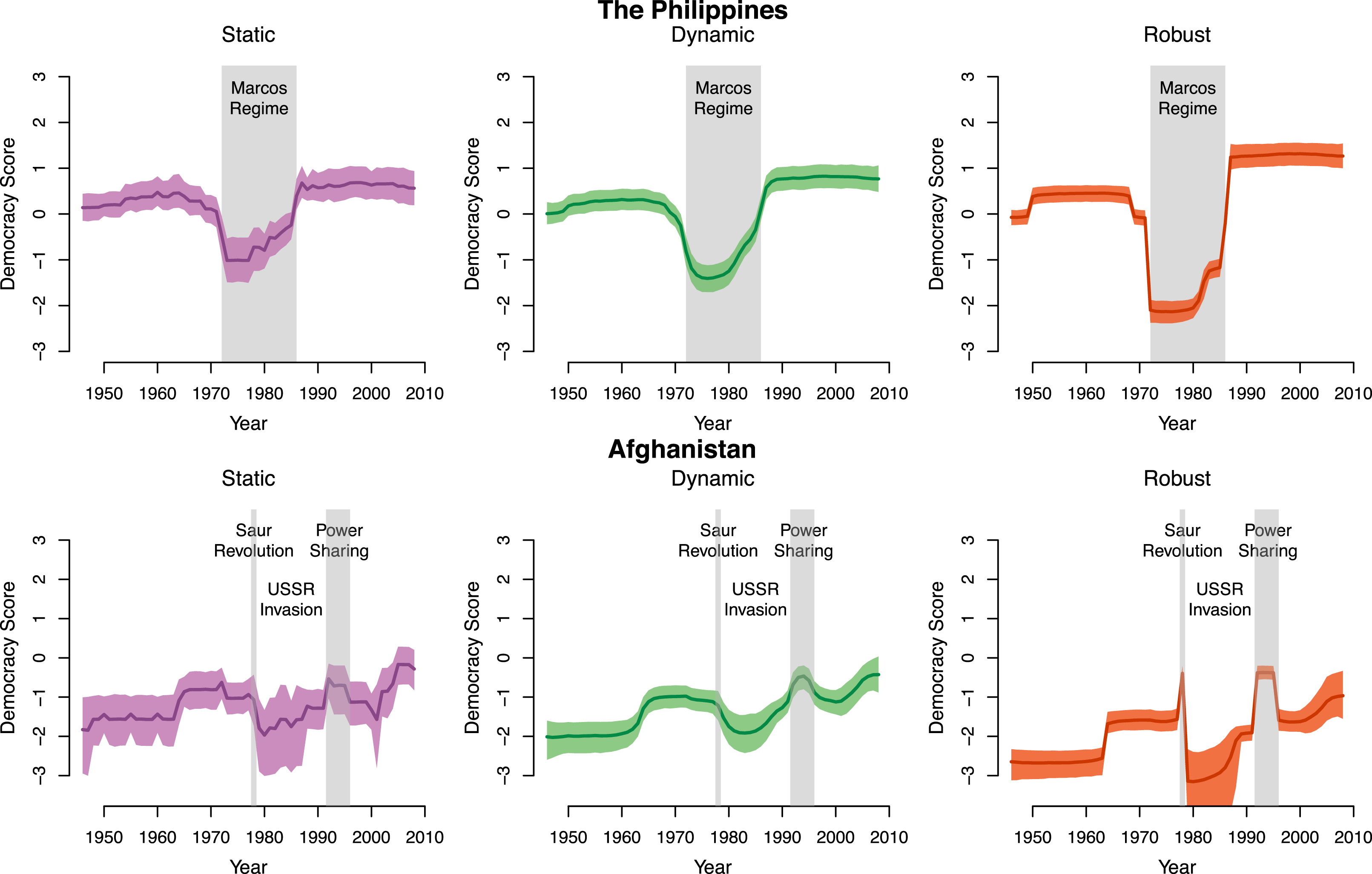
Next, we reproduce and evaluate two common latent variables in political science: judicial voting preferences (Martin and Quinn Reference Martin and Quinn2002) and democracy (Pemstein, Meserve, and Melton Reference Pemstein, Meserve and Melton2010). We find that the estimates from the robust latent variable model reveal previously unobserved shocks and improve fit for both constructs. Substantively, the robust model provides evidence that judicial voting patterns sometimes change rapidly for a subset of Supreme Court justices. We also find that the robust model provides more precise estimates of democracy in response to sudden political events such as the imposition of martial law that occurred in the Philippines from 1972 through 1981 under the regime of Ferdinand Marcos and the short-lived Saur Revolution in Afghanistan in 1978. The analyses indicate that the robust latent variable model yields substantively meaningful insights not obtainable from existing latent variable modeling strategies.
1 Modeling Strategies and Simulation Analysis
We start by briefly discussing the static and dynamic modeling strategies and introducing the robust modeling alternative. We also outline a simple data generating process and the priors which we will use in a simulation analysis of the competing models.
We begin with a simple item response theory framework (IRT) with binary manifest variables.Footnote
1
The latent trait,
 $\unicode[STIX]{x1D703}_{\mathit{it}}$
exists for each unit,
 $i=1,\ldots ,N$
across each time period
 $t=1,\ldots ,T$
.
 $\unicode[STIX]{x1D703}_{\mathit{it}}$
is not observed directly, but determines the value of a series of manifest variables, or items,
 $y_{kit}$
, where
 $k=1,\ldots ,K$
indexes the number of items observed. Thus,
 $y_{itk}$
is the observed value for item
 $k$
for unit
 $i$
at time
 $t$
. For each item,
 $\unicode[STIX]{x1D6FC}_{k}$
and
 $\unicode[STIX]{x1D6FD}_{k}$
are estimated. These are commonly referred to as the “difficulty” and “discrimination” parameters, respectively and are analogous to an intercept and slope in traditional logit regression. The likelihood function takes the following form, where
 $\unicode[STIX]{x1D6EC}$
is the logistic function:
 $$\begin{eqnarray}\displaystyle {\mathcal{L}}=\mathop{\prod }_{i,t=1}^{N,T}\mathop{\prod }_{k=1}^{K}\unicode[STIX]{x1D6EC}(\unicode[STIX]{x1D6FC}_{k}-\unicode[STIX]{x1D6FD}_{k}\unicode[STIX]{x1D703}_{\mathit{it}})^{y_{itk}}(1-\unicode[STIX]{x1D6EC}(\unicode[STIX]{x1D6FC}_{k}-\unicode[STIX]{x1D6FD}_{k}\unicode[STIX]{x1D703}_{\mathit{it}}))^{1-y_{itk}}. & & \displaystyle \nonumber\end{eqnarray}$$
We place weakly informative, normal priors on the difficulty and discrimination parameters. In addition,
 $\unicode[STIX]{x1D6FD}_{k}$
, the difficulty parameter, is constrained to be greater than 0. This is a common identification constraint that resolves rotational invariance by preventing “flipping” where the likelihood from
 $\hat{\unicode[STIX]{x1D6FD}}_{k}$
and
 $\hat{\unicode[STIX]{x1D703}}_{\mathit{it}}$
is equal to the likelihood from
 $-\hat{\unicode[STIX]{x1D6FD}}_{k}$
and
 $-\hat{\unicode[STIX]{x1D703}}_{\mathit{it}}$
. All the items are then coded so that a 1 indicates increased levels of the latent trait, and a 0 decreased levels.Footnote
2
Formally our priors are:
 $$\begin{eqnarray}\displaystyle \unicode[STIX]{x1D6FC}_{k} & {\sim} & \displaystyle \text{N}(0,3)\nonumber\\ \displaystyle \unicode[STIX]{x1D6FD}_{k} & {\sim} & \displaystyle \text{HN}(0,3).\nonumber\end{eqnarray}$$
HN is the half-normal distribution, with support on
 $[0,\infty )$
. All models presented here share these priors on their item parameters.
1.1 Static Model
The three modeling strategies we present are differentiated by the prior information assigned to the latent variable. The static model, places a standard normal prior on all units for all time periods:
Static Model Prior
 $$\begin{eqnarray}\displaystyle \unicode[STIX]{x1D703}_{\mathit{it}} & {\sim}\text{N}(0,1)\quad \forall i=1,\ldots ,N\quad \& \quad \forall t=1,\ldots ,T. & \displaystyle \nonumber\end{eqnarray}$$
Estimates for each unit in each time period are therefore differentiated exclusively by the values of the manifest variables for that unit at that time period. This allows for sudden changes in the latent estimates in a unit between time periods. A shortcoming of this model is that it treats each observation as independent. In the case where the manifest variables contain sufficient information on the latent trait, this modeling strategy may not be problematic. Unfortunately, this is seldom the case when using social science data, where indicators are often coarse or missing. As a result, these indicators often do not contain sufficient information to differentiate between theoretically distinct units.
1.2 Standard Dynamic Model
To address temporal nonindependence in the data, many researchers use a dynamic prior for the latent trait (Martin and Quinn Reference Martin and Quinn2002; Kōnig, Marbach, and Osnabrügge Reference Kōnig, Marbach and Osnabrügge2013; Fariss Reference Fariss2014; Schnakenberg and Fariss Reference Schnakenberg and Fariss2014; Caughey and Warshaw Reference Caughey and Warshaw2015). The choice of a “random walk” prior on the latent variable is particularly common.
Researchers apply a standard normal distribution to the latent trait in the first observation period for every unit. For each subsequent time period, the prior is normally distributed with mean
 $\unicode[STIX]{x1D703}_{i(t-1)}$
, and an innovation standard deviation
 $\unicode[STIX]{x1D70E}$
which is either assigned by the researcher or, more commonly, estimated from the data. Here, we assign a weakly informative prior to
 $\unicode[STIX]{x1D70E}$
by using a half-normal distribution with standard deviation of 3 and mean 0.Footnote
3
Standard Dynamic Model Priors
 $$\begin{eqnarray}\displaystyle \unicode[STIX]{x1D703}_{i1} & {\sim} & \displaystyle \text{N}(0,1)\quad \forall i=1,\ldots ,N\nonumber\\ \displaystyle \unicode[STIX]{x1D703}_{\mathit{it}} & {\sim} & \displaystyle \text{N}(\unicode[STIX]{x1D703}_{i(t-1)},\unicode[STIX]{x1D70E})\quad \forall i=1,\ldots ,N\quad \& \quad \forall t=2,\ldots ,T\nonumber\\ \displaystyle \unicode[STIX]{x1D70E} & {\sim} & \displaystyle \text{HN}(0,3).\nonumber\end{eqnarray}$$
This strategy trades the assumption that observations are independent with the assumption that the latent trait will be correlated over time. As a result, estimates from dynamic models typically have less uncertainty because more information is used to estimate each latent variable. This also induces smoothing over time because changes between time periods are constrained. When researchers have theoretical reasons to expect that the latent trait is relatively slow-moving over time, both modeling features can be desirable. If, however, the latent trait is subject to rapid fluctuations or state changes between time periods, this temporal smoothing can produce biased estimates. The modeling strategy we introduce below is designed to address this problem while still accounting for temporal dynamics.
1.3 Robust Dynamic Modeling
Our alternative strategy draws on the robust modeling literature. Robust models, broadly defined, weaken the parametric assumptions common to standard statistical models as a means of accommodating unique data structures and the potential for influential outlying observations. One simple modification commonly used is the substitution of normally distributed errors with Student’s
 $t$
-distributed errors (Lange, Little, and Taylor Reference Lange, Little and Taylor1989; Lange and Sinsheimer Reference Lange and Sinsheimer1993; Gelman et al.
Reference Gelman, Carlin, Stern, Dunson, Vehtari and Rubin2014). A specific Bayesian approach to the use of the Student’s
 $t$
-distribution has been developed (Geweke Reference Geweke1993; Fonseca, Ferreira, and Migon Reference Fonseca, Ferreira and Migon2008). This strategy has been used to account for heterogeneity in growth models (Zhang et al.
Reference Zhang, Lai, Lu and Tong2013), ordinal choice models (Stegmueller Reference Stegmueller2013), and mixed effects models (Rosa, Gianola, and Padovani Reference Rosa, Gianola and Padovani2004) among others. Within our context, potential outliers are “shocks” where values of the true latent variable change suddenly within a unit’s time series. As a prior on the latent variable
 $\unicode[STIX]{x1D703}$
, the Student’s
 $t$
-distribution is less restrictive when estimating the temporal data generating process that relates to the latent trait with the observed manifest variables because it has greater density in the tails when compared to the standard normal distribution (for details on the Student’s
 $t$
-distribution see Supplementary Appendix A).
To develop a robust dynamic model, we set the prior for the first year in a particular time series to a standard normal distribution.Footnote
4
For every subsequent year, the prior then follows a Student’s
 $t$
-distribution, with four degrees of freedom. Setting the degrees of freedom to a relatively low value increases the density of the tails of the distribution which allows “extreme values” to be estimated from time period to time period. Thus, the model smooths estimates across time during periods of stability, but also allows for rapid changes in the latent trait during periods of volatility. In the cases presented here we set the degrees of freedom and estimate the scale parameter
 $\unicode[STIX]{x1D70E}$
. In the appendix we discuss an alternative model specification where we estimate the degrees of freedom parameter instead of
 $\unicode[STIX]{x1D70E}$
, as well as a model that jointly estimates both parameters. We find that this does not improve model fit while potentially compounding rotational identification concerns in some cases and being computationally more taxing. Because of this, we opt to set the degrees of freedom at a low value of four, as recommended by Gelman et al. (Reference Gelman, Carlin, Stern, Dunson, Vehtari and Rubin2014).
Robust Dynamic Model Priors
 $$\begin{eqnarray}\displaystyle \unicode[STIX]{x1D703}_{i1} & {\sim} & \displaystyle \text{N}(0,1)\quad \forall i=1,\ldots ,N\nonumber\\ \displaystyle \unicode[STIX]{x1D703}_{\mathit{it}} & {\sim} & \displaystyle \text{T}_{4}(\unicode[STIX]{x1D703}_{i(t-1)},\unicode[STIX]{x1D70E})\quad \forall i=1,\ldots ,N\quad \& \quad \forall t=2,\ldots ,T\nonumber\\ \displaystyle \unicode[STIX]{x1D70E} & {\sim} & \displaystyle \text{HN}(0,3).\nonumber\end{eqnarray}$$
1.4 Potential Alternatives
In addition to the robust model there are several alternative modeling strategies that could be used to accommodate temporal shocks. First, given an assumed data generating process that is a combination of a dynamic process and a static process a finite mixture modeling strategy might be a useful strategy. We assess such a model in Supplementary Appendix B and find that the mixture model is outperformed by the robust model in almost all cases.
Another potential strategy would be to employ a change-point model (Western and Kleykamp Reference Western and Kleykamp2004) or regime switching model (Hamilton Reference Hamilton2010). These models capture the intuition that there is a discrete change in the underlying process. However, estimating these types of models requires a priori attention to the number of expected change points and are commonly employed only in time-series analysis (e.g., Pang et al. Reference Pang, Friedman, Martin and Quinn2012) but have seen some use in panel data (e.g., Joseph et al. Reference Joseph, Wolfson, Du Berger and Lyle1997; Spirling Reference Spirling2007). One of the main modeling challenges is estimating the discrete number of change points. This issue is particularly intractable for the types of punctuated equilibrium processes discussed here where the number of shocks or change points that are likely to exist in a given time-series are not known ex ante and vary across panels. In the univariate case, there have been some very useful developments in models without a fixed number of change points (Santifort, Sandler, and Brandt Reference Santifort, Sandler and Brandt2013). Other alternatives also exist for continuous time latent variables that do not assume discrete time intervals (Tahk Reference Tahk2015) as well as latent growth models which provide a flexible framework for specific theoretically driven assumptions about latent change over time (Duncan and Duncan Reference Duncan and Duncan2004). Evaluating all of these models is beyond the scope of this paper but each offers important opportunities for generating new inferences about unobservable concepts.
1.5 Simulation Analysis
To evaluate model performance we simulate conditions where the true data generating process is known. We focus in particular on situations where there is some time-series structure to the underlying latent trait. We do not evaluate any models in which there are no temporal dependencies in the underlying data generating process (e.g., the static model) given our focus on improving modeling techniques for data with dynamic temporal structures. While latent traits are sometimes temporally independent and identically distributed, we focus on more common conditions when this is not the case. In all our simulations, the latent trait is drawn from a standard normal distribution in its first time period and follows a random-walk process with the probability of a “shock” thereafter. When a unit experiences a shock, it is re-drawn from a standard normal distribution, thus inserting “breaks” in the time-series such that the latent trait is subject to the possibility of rapid change. From these “latent” variables, we estimate binary manifest indicators that are recorded with error for each observation. With these data in place, we estimate variants of the static, dynamic, and robust models and evaluate their performance under a variety of conditions. Information on these analyses, along with additional information on the underlying data generating process are available in the appendix.Footnote 5 Here, we provide a brief overview of our findings.
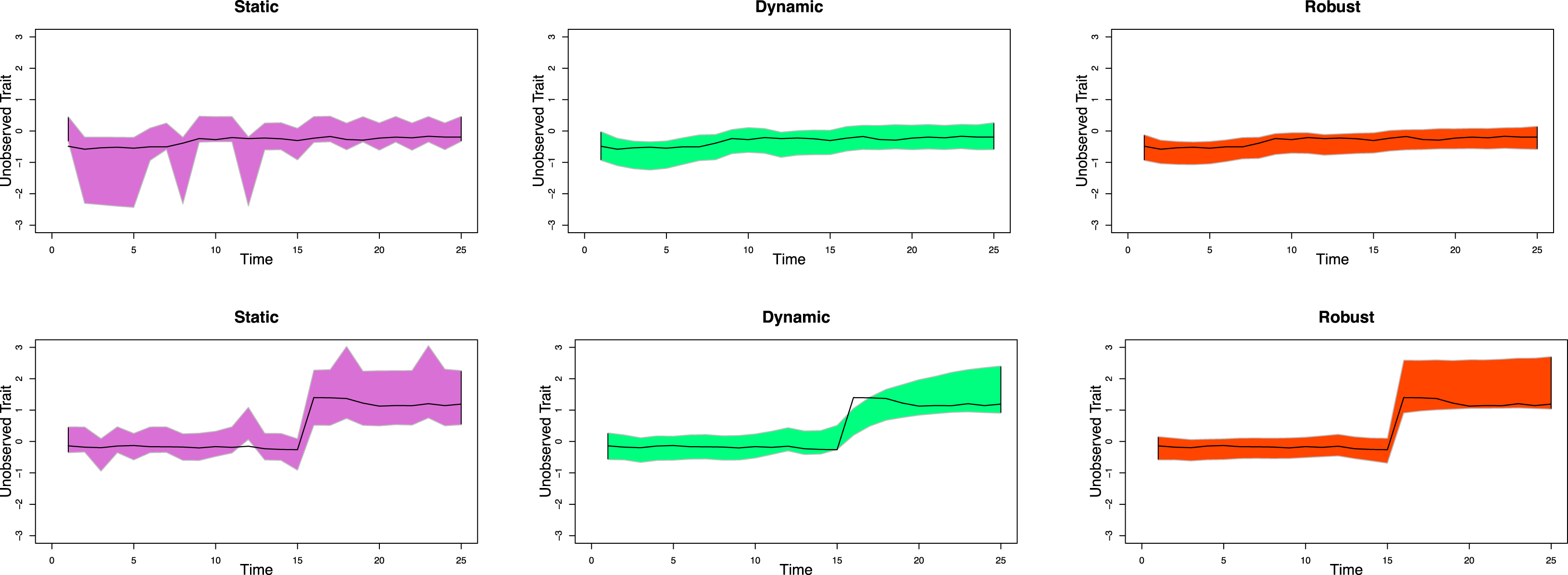
Figure 1 displays the differences in estimates of the latent trait from the static (left column), dynamic (center column), and robust (right column) for two sample units. These units were simulated with the probability of shock was set to 0.01, and the innovation standard deviation set to 0.05.Footnote 6 The first of these units (top panels) is representative of cases where the latent trait is relatively stable across time and does not experience a shock. The second (bottom panels) represents a case where a shock to the latent trait occurs after period 15.
Model Estimates Across Two Sample Units. Note: 95% Credible Intervals for two sample units using the four different modeling strategies. The true latent value is displayed with a dark line, and is the same in each row.

The efficiency loss in the static model is apparent for the unit that did not experience a shock. By efficiency loss, we mean a decrease in the amount of information contained in the estimate of the latent variable which translates into a flatter (and less informative) estimated probability density for each unit within the latent space. Although the true latent variable is within the credible interval of the static model across all time points, the credible intervals vary widely around it. This is because estimates at each time period are generated independently and so there is relatively limited information used in each time period. As expected, the dynamic and robust models generate lower estimates of uncertainty by leveraging time-series information in the data. Of particular note is that the use of the Student’s
 $t$
-distribution by the robust model does not lead to a significant increase in estimates of uncertainty relative to the dynamic model. The advantages of the robust model are apparent for the unit experiencing a shock. As before, the static model’s credible intervals are wide, but almost always capture the true estimate. By contrast, the dynamic model oversmooths the sudden changes in the time-series and therefore fails to produce accurate credible intervals over several time periods after the shock. The robust model, by contrast, produces relatively small credible intervals (in comparison to the static model) and is also capable of accounting for sudden changes to the true latent trait when the shock happens.
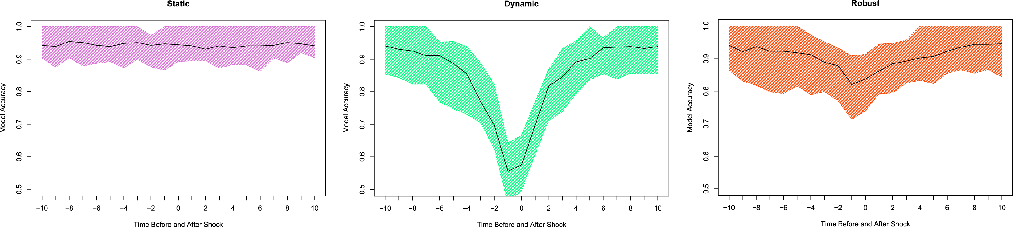
Next we show how these results generalize to many simulated units drawn from the described data generating process. In Figure 2 we plot the percentage of observations where the true latent trait value is contained within the 95% credible interval generated for each model as a function of the time before and after a shock to the latent trait (experienced at time
 $t=0$
). As expected, the static model performs particularly well using this metric due to its large credible intervals. More relevant for our purposes, the model performs equally well across all time periods, regardless of whether and when a unit experienced a shock. By contrast, the dynamic model performs well for units that have not recently experienced a shock, and poorly in the time of or proximate to a shock. This dip in accuracy is significantly mitigated, though not reduced entirely by the robust model. Taken together, the simulation analyses reported here and in the appendix indicate that the robust model is a viable alternative to standard dynamic modeling choices, particularly for latent traits subject to temporal volatility.
Model Accuracy in Time Surrounding Shocks to the Latent Variable. Note: The percentage of times the true latent variable is within 95% credible intervals. The horizontal axis is the distance away from the nearest shock. We omit a small number of observations that were within three time periods of two shocks. A distribution of values is estimated by generating 50 different simulated datasets—the bounds show the 20th and 80th percentile.

2 Substantive Applications
We now assess how the robust latent variable model performs using data from two important applications of latent variable models: a model of judicial ideology from Martin and Quinn (Reference Martin and Quinn2002) who originally used a dynamic model; and a model of democracy from Pemstein, Meserve, and Melton (Reference Pemstein, Meserve and Melton2010) who originally used a static model. For each, we estimate the original models and compare these original modeling strategies to the robust latent variable model. We assess model fit using the Widely Available Information Criterion (WAIC), posterior predictive checks, and visual assessments of well-known cases.Footnote 7
2.1 Martin and Quinn (Reference Martin and Quinn2002)
Martin and Quinn (Reference Martin and Quinn2002) design a latent variable model to measure United States Supreme Court justice ideology. The units are Supreme Court justice years and the items are the votes that each justice cast in a particular case. Each vote is coded zero or one depending on whether it overturns or affirms a lower court decision. Justices serve for multiple years, and Martin and Quinn (Reference Martin and Quinn2002) use a dynamic model with random walk priors to model the position of the justices over time. We replicate this model using the data made available on their website which extends the timespan of the original model to contain the years 1937–2015.
The sparsity of data along with a lack of clear polarity for votes required Martin and Quinn (Reference Martin and Quinn2002) to achieve identification through two modeling decisions. First, a subset of justices are assigned strong priors to allow them to act as anchors within the policy space. In addition, because of a sparsity of data they—after some experimentation—fix the value of the innovation variance (
 $\unicode[STIX]{x1D70E}^{2}$
) to 0.1.Footnote
8
Fixing the value of
 $\unicode[STIX]{x1D70E}^{2}$
warrants some additional discussion before proceeding. Often researchers estimate this parameter directly from the data, but sparse data structures such as this sometimes lead research to fix
 $\unicode[STIX]{x1D70E}^{2}$
. This value must be chosen carefully. When
 $\unicode[STIX]{x1D70E}^{2}\rightarrow \infty$
, the model will produce estimates for each period of time independently. Assigning
 $\unicode[STIX]{x1D70E}^{2}$
a value that is too large may produce a model that is not rotationally identified in cases where there are no expectations about the direction of the relationship between items and the latent trait. When
 $\unicode[STIX]{x1D70E}^{2}=0$
, the dynamic model will produce a single time-invariant estimate of the latent trait. Setting
 $\unicode[STIX]{x1D70E}^{2}$
to a value that is too small therefore ignores temporal variation of the latent trait. For a standard dynamic model, this is equivalent to fitting a flat line to a time-series.
The robust model is no less sensitive to these modeling decisions and shares many of the same properties as the standard dynamic model. One important exception, is that as
 $\unicode[STIX]{x1D70E}^{2}$
approaches zero, the robust model may fit an approximately stepwise function to smooth linear trends in the latent trait. This would result in the appearance of shocks in a time-series where none is present.Footnote
9
We therefore recommend practitioners estimate the value of
 $\unicode[STIX]{x1D70E}^{2}$
directly from the data when possible. If this parameter must be fixed, we recommend researchers evaluate model performance using multiple values of
 $\unicode[STIX]{x1D70E}^{2}$
. At each step, practitioners should evaluate model performance through a variety of metrics including those employed here: fit statistics such as WAIC; posterior predictive checks (particularly in times surrounding the “shocks” identified by the robust model); and visual inspection of the data.
We use a prior assignment and identification strategy similar to Martin and Quinn (Reference Martin and Quinn2002), including setting the innovation variance to 0.1 for all justices except Douglas and providing informed priors around a subset justices for their initial year on the court. In addition, because we use a more expansive dataset than originally employed by Martin and Quinn (Reference Martin and Quinn2002) we impose two additional priors on justices at the very end or very beginning of the time-series: Samuel Alito is given a prior on
 $\unicode[STIX]{x1D703}$
centered at 1.5 and Hugo Black is given a prior on
 $\unicode[STIX]{x1D703}$
centered at
 $-3$
. To ensure rotational identification we constrain some justices to be strictly positive or negative.Footnote
10
Finally, as in Martin and Quinn (Reference Martin and Quinn2002) we find that Douglas’s extremely limited and liberal voting pattern leads to near separation so we tighten the innovation variance to 0.0001, slightly tighter than the 0.001 imposed by Martin and Quinn (Reference Martin and Quinn2002). In the robust model we set the scale parameter in the Student’s
 $t$
-distribution so that the overall innovation variance is 0.1 given a Student’s
 $t$
-distribution with four degrees of freedom.Footnote
11
We evaluate model fit through posterior predictive checks (Gelman and Hill Reference Gelman and Hill2007; Gelman et al. Reference Gelman, Carlin, Stern, Dunson, Vehtari and Rubin2014). We sample from the posterior distribution of the parameter estimates generated from each model and use these values to make predictions about the votes cast by justices in each of the cases heard during their tenure. For every draw, we compute the proportion of justice decisions correctly predicted by each model. The robust model accurately predicts Supreme Court decisions 72.95% of the time, while the dynamic model generates accurate estimates 72.77% of the time. Although this is a substantively small difference, it is probabilistically distinguishable from 0. The fact that the robust model’s improvement is modest should be unsurprising, as the comparative advantage of this model pertains to the relatively small subset of instances where a Supreme Court justices’ voting position suddenly changes between years. Nevertheless, the improvement in predictive power is substantively meaningful for the subset of cases that seem to experience rapid fluctuations.
We estimate WAIC as a second means of comparing the models. WAIC is a fully Bayesian alternative to DIC and is asymptotically equal to Bayesian Leave-One-Out Cross-Validation. WAIC estimates the expected log pointwise predictive density (LPPD)Footnote 12 by estimating the LPPDFootnote 13 and correcting it by the number of effective parameters (Furr Reference Furr2017; Vehtari, Gelman, and Gabry Reference Vehtari, Gelman and Gabry2016). When estimating the expected model performance on new data, it is necessary to determine the form that hypothetical out-of-sample data will take (Gelman et al. Reference Gelman, Carlin, Stern, Dunson, Vehtari and Rubin2014). In this context, we evaluate out-of-sample performance in terms of new realizations of a particular justice’s decision on existing court cases. The LPPD is therefore calculated using the likelihood of a judicial decision, given each judge’s latent preference. The effective numbers of parameters correction are estimated using the summation of the variance of the log prediction density for each vote.Footnote 14
The difference in the WAIC scores provides evidence that the robust model is outperforming the original dynamic model. The estimate of WAIC for the dynamic replication is 46,852, reported on the deviance scale. The robust model improves on this, with a WAIC of 46,647. This is a difference of 205 with a standard error of 15.6—the robust model better fits the data than does the dynamic model.
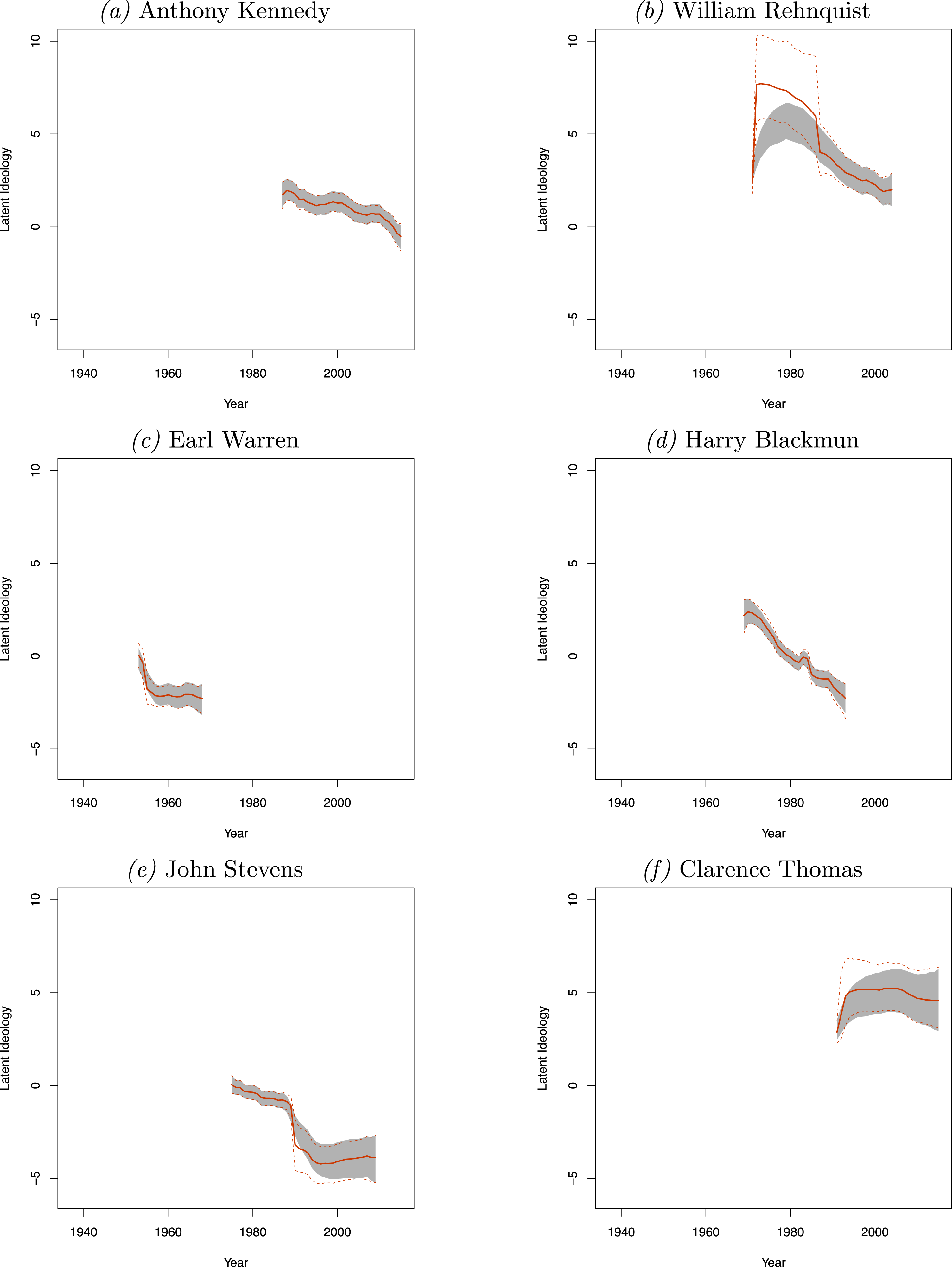
To demonstrate the substantive value of the robust model, we conduct a brief investigation of estimates for a subset of Supreme Court justices using visual evidence in Figure 3. We include (in the shaded area) the output from the dynamic model estimated by Martin and Quinn (Reference Martin and Quinn2002). One important contribution generated from the original model was confirmatory evidence that Supreme Court justice preferences changed meaningfully over time (Martin and Quinn Reference Martin and Quinn2002, Reference Martin and Quinn2007). Our results corroborate this finding, and for most justices there is little difference in the dynamic and robust model estimates.
Sample of Judicial Ideology—Robust and Martin and Quinn Scores. Note: Two sets of judicial ideology scores based on data from Martin and Quinn (Reference Martin and Quinn2002). These models are estimated using two different versions of the latent variable model (robust and dynamic). The robust model is represented by the solid black line for the median value and the dashed lines for the 2.5 and 97.5 credible interval. The dynamic model is represented by the shaded area, which is the 2.5 to 97.5 credible interval.

Yet, the smoothing pattern imposed by the dynamic modeling structure employed by the original authors also precludes the possibility that justice preferences may change rapidly. That a justice may suddenly become more liberal or conservative in their decision-making may seem unlikely. Nevertheless, we find evidence of such changes in a small, but substantively interesting set of cases. A brief examination suggests these rapid fluctuations are not simply a modeling artifact. For example, William Rehnquist’s score suddenly becomes more liberal in 1987. This was the first full year in which Rehnquist served as Chief Justice and it is plausible that this change to the composition of the court led to a commensurate change in Rehnquist’s voting patterns. As an additional validity check, we also consulted a criterion variable generated by Epstein et al. (Reference Epstein, Segal, Spaeth and Walker1996) that records a justice’s voting pattern on a similar liberal-conservative spectrum. These authors also identify a rapid change in Rehnquist’s voting pattern, which indicates that this shift reflected real-world changes and is not simply an artifact of our modeling assumptions.
Though we do not offer causal interpretation or explanation for these changes, investigating rapid shifts in voting patterns is a promising area for future research. For example, strategic explanations for Supreme Court justice behavior suggest that voting patterns are a function of both a justice’s underlying political ideology and the anticipated actions and preferences of their colleagues and external political entities (Epstein and Knight Reference Epstein and Knight2013). Scholars adhering to this framework might argue that Rehnquist’s changed voting patterns after becoming chief justice were a result of strategic incentives. Prior to becoming Chief Justice, Rehnquist was known for consistently voting with Chief Justice Burger, in part to maintain their positive collegial relationship (Woodward and Armstrong Reference Woodward and Armstrong1979). As Chief Justice, however, Rehnquist selected the majority opinion writer for all cases in which he was also in the majority. This provides him with an avenue for substantively impacting court decisions, even in cases where he may have otherwise been inclined to vote with the minority. We are agnostic to the validity of these potential explanations. Nonetheless, we find it heartening that the new patterns uncovered by the robust model appear to corroborate some existing arguments. In short, the robust model estimates help bring evidence about such cases to the forefront by accommodating rapid changes—an insight that would remain unobserved due to the smoothing induced by standard dynamic modeling procedures.
2.2 Pemstein, Meserve, and Melton (Reference Pemstein, Meserve and Melton2010)
Pemstein, Meserve, and Melton (Reference Pemstein, Meserve and Melton2010) generate country-year estimates of democracy using a static latent variable model that uses ten indicators of democracy. These items include: Polity (Marshall, Jaggers, and Gurr Reference Marshall, Jaggers and Gurr2006); Freedom House (2007); Polyarchy (Coppedge and Reinicke Reference Coppedge, Reinicke and Inkeles1991); Bollen (Reference Bollen2001); Vanhanen (Reference Vanhanen2003); Arat (Reference Arat1991); Political Regime Change (PRC) (Gasiorowski Reference Gasiorowski1996); Bowman, Lehoucq, and Mahoney (Reference Bowman, Lehoucq and Mahoney2005) (BLM); and Przeworski et al. (Reference Przeworski, Alvarez, Cheibub and Limongi2000) (PACL). Each of these items are assumed to be a unique approximation of a given country’s latent level of democracy. While the items are measured on different scales, the authors treat each as ordinal when linking the items to the latent level of democracy through an ordinal probit function. The model is identified through the application of a standard normal prior distribution on the latent level of democracy and uninformative, uniform priors applied to the cut-point parameters for each item. We depart from the original model slightly by linking the items to the latent trait using the ordered logit, rather than ordered probit function. We also use item-specific slope parameters, instead of item-specific variances, to account for the differences in precision of each item. These modifications do not lead to substantial changes in model estimates—the correlation between our replicated estimates of democracy and the original estimates is 0.987. In addition, we also estimate dynamic and robust variants of the original model.
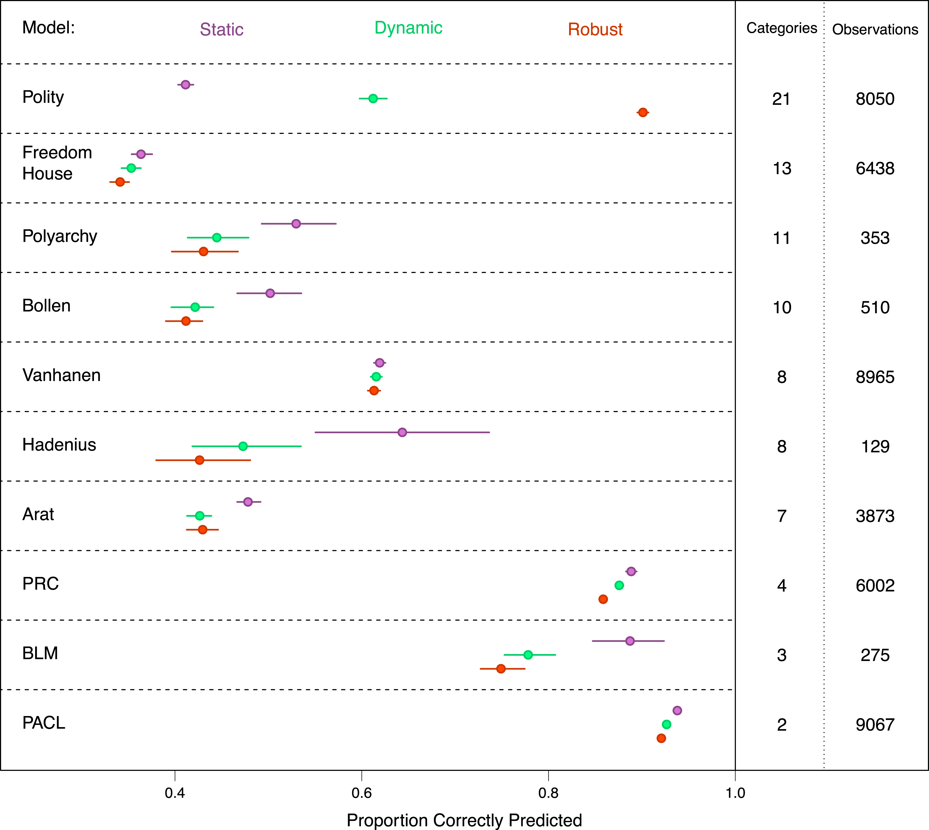
Posterior Predictive Checks—Pemstein, Meserve, and Melton (Reference Pemstein, Meserve and Melton2010) Replication. Note: This plot displays each models performance in accurately predicting the values of the ten democracy indicators used to generate model estimates. 500 sets of predictions were randomly drawn from the posterior distributions produced by each model. The horizontal axis reports the percent of cases correctly predicted. Models are displayed along the vertical axis. Dots correspond to the median value from the set of predictions, while solid lines denote the 2.5 and 97.5 percentile values of each models performance. The static model estimates are colored purple, the dynamic model is colored green, and the robust model orange.

As with the Martin and Quinn (Reference Martin and Quinn2002) replication, we also calculate WAIC for each of the three models. The WAIC is 93,267, 79,237, and 65,082 for the static, dynamic, and robust models respectively. The difference between the static model and robust model is 28,185 with a standard error of 358.8. The difference between the dynamic model and the robust model is 14,029 with a standard error of 247.7. In terms of predictive accuracy, the robust model is a substantial improvement upon both alternatives.
Figure 4 reports the posterior predictive checks used to assess model performance. With some exception, we find that each of the models produce less accurate predictions for indicators with many categories, and more accurate predictions for indicators with few categories. The difference in model performance is greatest for the polity indicator—here the static model correctly predicts polity scores for 41 percent of observations, the dynamic model does so for 61 percent, and the robust model does so for 90 percent. The static model does, however, fair best when predicting Polyarchy, Bollen, Arat, and BLM, though the differences in accuracy are less stark for these variables. The models produce similar accuracy figures for the remaining indicators (Freedom House, Vanhanen, PRC, and PACL). In Appendix F, we evaluate how the models perform when predicting annual change for seven democracy indicators. The robust model performs as well or better for every indicator. It also continues to outperform the static model for Polity.
A brief examination of historical cases that experience shocks—displayed in Figure 5—offers additional support for the robust model. The dynamic model produces narrower credible intervals than the static model, but oversmooths and anticipates the sudden changes to the level of democracy in these two countries. For the Philippines, the robust model, identifies a steep decrease in the level of democracy in 1972 when Ferdinand Marcos declares martial law and the onset of an autocratic regime. The robust model also estimates a notable increase after 1981, when marital law ended, and another dramatic increase in 1987 with the revolution that expelled Marcos from power. The robust dynamic model is also able to capture sudden changes for the case of Afghanistan. The model even captures the Saur Revolution, which occurred in 1978 and was quickly followed by the Soviet invasion in 1979. This sudden and short-lived institutional change is not observable in any of the other models which again highlights the pitfalls associated with the oversmoothing produced by the standard dynamic approach and constitutes an important validity check.
The Philippines and Afghanistan, Latent Democracy Score—Pemstein, Meserve, and Melton (Reference Pemstein, Meserve and Melton2010) Replication. Note: Estimates of democracy are displayed for the Philippines (first row) and Afghanistan (second row). Mean estimates and 95 percent credible intervals are indicated with a solid line and shaded region. For the case of the Philippines, the robust model is able to clearly distinguish between the periods before, during, and after the Marcos regime. For the case of Afghanistan, the robust model is able to clearly capture the short-lived Saur Revolution in Afghanistan that occurred in 1978 and was quickly followed by the Soviet invasion in 1979.

3 Discussion
Through simulated data and the reproduction of two existing latent variable models, we have explored how a relatively simple modification to the dynamic latent variable model increases the validity of the estimates of these variables when temporal shocks are present. Across a variety of metrics, the robust dynamic model outperforms existing modeling techniques when the latent traits are subject to volatility. Nevertheless, there is no guarantee that any single modeling strategy will be equally well suited for use with all data types or for estimating different latent concepts. The assumptions of the measurement model will influence the conclusions researchers draw both about the underlying theoretical concept of interest, as well as the empirical linkages between these concepts and other phenomena. We therefore suggest researchers estimate both dynamic and robust models and then assess the relative validity of the latent estimates with as many different evaluation tools as possible. Fit statistics, posterior predictive checks, and visual analysis of the temporal patterns of several well-known cases allowed us to evaluate the competing models without relying on a single statistical tool. Overall, the robust latent variable model reduces the bias associated with dynamic models without sacrificing efficiency, which has lead to new insights about the dynamic patterns of judicial ideology and democracy.
Supplementary material
For supplementary material accompanying this paper, please visit https://doi.org/10.1017/pan.2019.1.