2.1. Large-scale motions

Giving a rigorous definition of large-scale motions is a challenge. One of the most common definitions uses a Fourier cut-off filter in time, or one of homogeneous spatial directions, or a combination of such filters. The alternatives include the bi-dimensional version of the empirical mode decomposition (Huang et al. Reference Huang, Shen, Long, Wu, Shih, Zheng, Yen, Tung and Liu1998) first applied in the present context in Agostini & Leschziner (Reference Agostini and Leschziner2014) and the decomposition based on the hierarchical random additive process (Yang, Marusic & Meneveau Reference Yang, Marusic and Meneveau2016). Each of these methods requires additional decisions to be made to define the filter uniquely. The QSQH theory (Zhang & Chernyshenko Reference Zhang and Chernyshenko2016) circumvents this difficulty by specifying the properties of the large-scale filter that are required for the theory to be valid. Then the theory is built without defining the filter itself. To apply the theory to a particular flow one can then select the filter satisfying these properties at least approximately. An extensive investigation of filter selection was done by Zhang (Reference Zhang2019). Alternatively, one can derive useful relationships on the basis only of the assumption that such a filter exists, without specifying the filter explicitly. This approach will be followed in this paper. The reasons why this is at all possible are discussed in Chernyshenko et al. (Reference Chernyshenko, Zhang, Butt and Beit-Sadi2019), but this issue is far outside the scope of the present paper.

A large-scale filter is an operator that if applied to any scalar or vector-valued function of time and spatial coordinates gives the large-scale component of that function. We will denote the large-scale component with a subscript ‘$L$’. Thus, $f_L(t,\boldsymbol {x})={L} f(t,\boldsymbol {x})$, where ${L}$ is the large-scale filter.

The QSQH theory assumes that L has the following properties. For any constants $a$ and $b$ and functions $f (t,\boldsymbol {x})$ and $g(t,\boldsymbol {x})$:

P1. Linearity,

(2.1)\begin{equation} {L} (af + bg) = a{L} f + b{L} g. \end{equation}

P2. Invariance of averages: the averaged variables are large scale,

(2.2)\begin{equation} {L} \left\langle{f }\right\rangle = \left\langle{f }\right\rangle. \end{equation}

P3. Projection property: the large-scale filter does not change an already large-scale-filtered function,

(2.3)\begin{equation} {L} {L} f = {L} f. \end{equation}

P4. Commuting with averaging,

(2.4)\begin{equation} \left\langle{{L} f }\right\rangle = {L} \left\langle{f }\right\rangle. \end{equation}

P5. Scale-separation property: applying the large-scale filter to any function of $t$, $\boldsymbol {x}$ and other arguments that are large-scale-filtered variables is equivalent to averaging with the large-scale arguments held constant,

(2.5)\begin{equation} {L} f (t,\boldsymbol{x}, Lg_1, \ldots, {L} g_n) = \left\langle{f (t,\boldsymbol{x},\xi_1,\ldots,\xi_n )}\right\rangle_{\xi_1={L} g_1,\ldots,\xi_n={L} g_n}. \end{equation}

The fifth property expresses the reason why the QSQH theory might describe the scale interaction in near-wall turbulence. Property 5 will be satisfied to the extent to which the characteristic dimensions of the large scales are much larger than the characteristic dimensions of small scales.

2.2. Non-dimensional units

Wall friction $\boldsymbol {\tau }^*$ and its large-scale component $\boldsymbol {\tau }_L^*={L} \boldsymbol {\tau }^*$ are vectors parallel to the wall. Similar to the friction velocity, we introduce the large-scale friction velocity

(2.6)\begin{equation} u_{\tau_L}^*=\sqrt{|\boldsymbol{\tau}_L^*|/\rho^*}. \end{equation}

Note that unlike the friction velocity, $u_{\tau _L}^*$ is a function of time and the wall-parallel coordinates, and, where the statistical interpretation is used, it is a random function. In the rest of the paper all quantities will be made non-dimensional using the average large-scale friction velocity $\left \langle {u_{\tau _L}^*}\right \rangle$. Namely, the non-dimensional velocity, coordinates and time are

(2.7a–c)\begin{equation} \boldsymbol{u}=\boldsymbol{u}^*/\left\langle{u_{\tau_L}^*}\right\rangle, \quad \boldsymbol{x} = \boldsymbol{x}^* \left\langle{u_{\tau_L}^*}\right\rangle/\nu^*, \quad t = t^* {\left\langle{u_{\tau_L}^*}\right\rangle}^2/\nu^*, \end{equation}

where starred variables are dimensional. In these units the fluctuation of the large-scale friction velocity $u'_{\tau _L}=u_{\tau _L}-1$. The friction velocity is $u_\tau =\sqrt {\left \langle {\tau }\right \rangle }=\sqrt {\left \langle {\tau _L}\right \rangle }=\sqrt {\left \langle {u_{\tau _L}^2}\right \rangle }=\sqrt {1+\left \langle {u'^2_{\tau _L}}\right \rangle }$, where we used the fact that $\left \langle {\tau }\right \rangle =\left \langle {\tau _L}\right \rangle$ by a combination of properties P2 and P4.

The variables in the usual wall units and the non-dimensional units thus introduced are therefore related as

(2.8a–c)\begin{equation} \boldsymbol{u}^+=\boldsymbol{u}/u_\tau=\boldsymbol{u}/\sqrt{1+\left\langle{u'^2_{\tau_L}}\right\rangle},\quad \boldsymbol{x}^+=\boldsymbol{x}\sqrt{1+\left\langle{u'^2_{\tau_L}}\right\rangle}, \quad t^+=t\left(1+\left\langle{u'^2_{\tau_L}}\right\rangle\right). \end{equation}

They are very close quantitatively, at least for moderate ${\textit {Re}}$, when the fluctuations of the magnitude of large-scale motions are small.

2.3. Formulation of the QSQH hypothesis

If the large-scale component $\boldsymbol {\tau }_L$ were independent of time and the wall-parallel coordinates, while the small-scale component had zero time average, one could use wall units based on $\boldsymbol {\tau }_L$, which would coincide with the mean wall friction, and expect that near the wall the flow statistics expressed in thus defined wall units would be (approximately) independent of ${\textit {Re}}$ and other factors, including the dimensional value of $\boldsymbol {\tau }_L^*.$ The QSQH theory assumes that the same remains true even when $\boldsymbol {\tau }_L$ is dependent on time and the wall-parallel coordinates. The physical meaning of this hypothesis is therefore that the near-wall flow adjusts to the large-scale wall friction as if it were constant in time and homogeneous in space.

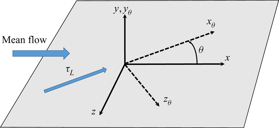
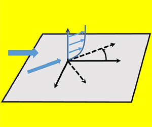
The large-scale component of the wall friction $\boldsymbol {\tau }_L(t,x,z)$ is a vector. A local coordinate system with an axis along the direction of $\boldsymbol {\tau }_L(t,x,z)$ shown in figure 1 and the coordinate system $x,y,z$ aligned with the mean flow direction are related by the formulae

(2.9a–c)\begin{gather} x_\theta=x\cos\theta -z \sin\theta,\quad y_\theta=y,\quad z_\theta=x\sin\theta+z\cos\theta, \end{gather}

(2.10a–c)\begin{gather} u=u_\theta\cos\theta +w_\theta \sin\theta,\quad v=v_\theta,\quad w={-}u_\theta\sin\theta+w_\theta\cos\theta,\end{gather}

where $\theta$ is the angle between the direction of the mean wall friction and the large-scale wall friction.

Figure 1.

The coordinate systems: $x$ is in the direction of the mean flow, $x_\theta$ is in the direction of the large-scale component of the wall friction, $y$ and $y_\theta$ coincide, being in the wall-normal direction, $z$ and $z_\theta$ are in the wall plane and perpendicular to $x$ and $x_\theta$, respectively. The angle $\theta$ is measured clockwise if looked at from above the wall.

The main relationships of the extended QSQH theory are

(2.11)\begin{gather} u_\theta(t,x_\theta,y_\theta,z_\theta)=u_{\tau_L}\tilde{u}(\tilde{t},\tilde{x},\tilde{y},\tilde{z}),\end{gather}

(2.12)\begin{gather} v_\theta(t,x_\theta,y_\theta,z_\theta)=u_{\tau_L}\tilde{v}(\tilde{t},\tilde{x},\tilde{y},\tilde{z}),\end{gather}

(2.13)\begin{gather} w_\theta(t,x_\theta,y_\theta,z_\theta,)=u_{\tau_L}\tilde{w}(\tilde{t},\tilde{x},\tilde{y},\tilde{z}),\end{gather}

(2.14a–d)\begin{gather} \tilde{t}=tu_{\tau_L}^2,\quad \tilde{x}=x_\theta u_{\tau_L},\quad \tilde{y}=y_\theta u_{\tau_L},\quad \tilde{z}=z_\theta u_{\tau_L}, \end{gather}

(2.15)\begin{gather} P[u_{\tau_L},\theta,\tilde{u}, \tilde{v}, \tilde{w},{\textit{Re}}]= P_{o}[u_{\tau_L},\theta,{\textit{Re}}]P_{u}[\tilde{u}, \tilde{v}, \tilde{w}],\end{gather}

where $P$ is the joint probability density functional of the functions $u_{\tau _L}(\cdot )$, $\theta (\cdot )$, $\tilde {u}(\cdot )$, $\tilde {v}(\cdot )$, $\tilde {w}(\cdot )$ and $P_{o}$ and $P_{u}$ are marginal probability density functionals of $u_{\tau _L}(.)$, $\theta (.)$ and $\tilde {u}(.)$, $\tilde {v}(.)$, $\tilde {w}(.)$, respectively. Similar to the expression of the classical universality hypothesis (1.2), the absence of ${\textit {Re}}$ from the arguments of $P_{u}$ is meant to indicate that the functions $\tilde {u}(.)$, $\tilde {v}(.)$ and $\tilde {w}(.)$ are universal in the sense that their statistical properties are independent of ${\textit {Re}}$ and of other global flow properties.

Equation (2.15) means that the set of functions $u_{\tau _L}(\cdot )$, $\theta (\cdot )$ and the set of functions $\tilde {u}(\cdot ),$ $\tilde {v}(\cdot )$, $\tilde {w}(\cdot )$ are statistically independent. To clarify this, this implies, for example, implies that for any non-random constant numbers $\xi _1,\xi _2,\xi _3,\xi _4,t,x$ and $z$, the value of $\tilde {u}(\xi _1,\xi _2,\xi _3,\xi _4)$ and the value of $u_{\tau _L}(t,x,z)$ are statistically independent, which in turn implies that their correlation is zero. Note however that, for constant $t,x,y,z$, the values of $\tilde {u}(\tilde {t},\tilde {x},\tilde {y},\tilde {z})$ and $u_{\tau _L}(t,x,z)$ are not statistically independent, since in this case $\tilde {t},\tilde {x},\tilde {y},\tilde {z}$ depend on $u_{\tau _L}$. Note also that though (2.11)–(2.14a–d) do not involve $\theta$ explicitly, the statistics of $u,$ $v$ and $w$ depend on the statistics of $\theta$ since it enters (2.9a–c) and (2.10a–c).

If $u_{\tau _L}$ and $\theta$ were not fluctuating then $u_{\tau _L}$ would be equal to 1 due to our choice of the non-dimensional variables, the averaged large-scale friction would be equal to the mean friction, our non-dimensional units would coincide with the wall units, $\tilde {u}, \tilde {v}, \tilde {w}$ would be the velocity components in wall units $u^+, v^+, w^+$, and $\tilde {t},\tilde {x},\tilde {y},\tilde {z}$ would be the time and coordinates in wall units $t^+, x^+,y^+,z^+$. Equations (2.11)–(2.14a–d) are the QSQH theory refinement suggested, although not explicitly formulated, by Zhang & Chernyshenko (Reference Zhang and Chernyshenko2016). If only the magnitude of the wall friction but not its direction fluctuates, that is, $\theta =0$, then (2.11) coincides with (5) in Chernyshenko et al. (Reference Chernyshenko, Marusic and Mathis2012), and (2.12), (2.13) are the assumptions implied by Agostini & Leschziner (Reference Agostini and Leschziner2019b).

The variables marked with a tilde are the QSQH analogue of the variables marked with a plus in the classical universality paradigm. These ‘tilde’ variables are a kind of ‘plus’ variable, but built on the fluctuating magnitude and direction of the large-scale component of skin friction instead of the constant mean skin friction.

Note also that as it follows from their definition and the filter property P5, (2.5), $u_{\tau _L}$ and $\theta$ are large-scale functions, so that ${L}u_{\tau _L}=u_{\tau _L}$ and ${L}\theta =\theta$.

The QSQH theory can be thought of as consisting of three parts. The first part is a rigorous mathematical theory of the relations between vector-valued functions $\boldsymbol {u}(t,x,y,z)$ and $\boldsymbol {\tau }_L(t,x,z)$, functions $u_{\tau _L}(t,x,z)=\sqrt {|\boldsymbol {\tau }_L(t,x,z)}|$ and $\theta (t,x,z)$, and an operator ${L}$ satisfying the relations (2.1)–(2.5), (2.9a–c)–(2.10a–c), (2.11)–(2.15). The second part, a physical hypothesis of quasi-steadiness, is the hypothesis that there exists such an operator ${L}$ that the velocity field of a real fluid flow satisfies, at least approximately, the above conditions. The third part, a physical hypothesis of universality, is the hypothesis that the statistical properties of the functions $\tilde {u}(\cdot ,\cdot ,\cdot )$, $\tilde {v}(\cdot ,\cdot ,\cdot )$ and $\tilde {w}(\cdot ,\cdot ,\cdot )$ are at least approximately the same for all real flows with sufficiently large ${\textit {Re}}$ independently of other large-scale factors such as the steady pressure gradient or smooth wall geometry. With both physical hypotheses accepted, the QSQH theory allows us to express the statistical properties of the total velocity field in terms of the statistical properties of $u_{\tau _L}$ and $\theta$, which depend on ${\textit {Re}}$ and other large-scale factors, and the universal statistical properties of $\tilde {u}(\cdot ,\cdot ,\cdot )$, $\tilde {v}(\cdot ,\cdot ,\cdot )$ and $\tilde {w}(\cdot ,\cdot ,\cdot )$.

2.4. Simplifications and basic relations

If only the statistics that are one-point in wall-parallel directions and time are considered, shifting the coordinate origin to the point and time of interest makes $t=x=x_\theta =z=z_\theta =0$. Then with zero arguments omitted (2.9a–c)–(2.13) reduce to

(2.16)\begin{gather} u/u_{\tau_L}=\tilde{u}(yu_{\tau_L})\cos\theta +\tilde{w}(yu_{\tau_L}) \sin\theta, \end{gather}

(2.17)\begin{gather}v/u_{\tau_L}=\tilde{v}(yu_{\tau_L}), \end{gather}

(2.18)\begin{gather}w/u_{\tau_L}={-}\tilde{u}(yu_{\tau_L})\sin\theta+\tilde{w}(yu_{\tau_L})\cos\theta. \end{gather}

Further considerations in the present paper will refer to this case. Once again, we use ensemble averaging, with the understanding that with the ergodicity assumption the ensemble averages are equal to time and homogeneous direction averages, to which the obtained results will therefore also apply.

When the large-scale wall friction does not fluctuate and is the same everywhere on the wall, $\theta =0$, $u_{\tau _L}=1$, $x=\tilde {x}$, $y=\tilde {y}$, $z=\tilde {z}$, $u=\tilde {u}$, $v=\tilde {v}$ and $w=\tilde {w}$. A natural assumption that the mean velocity $(U,V,W)$ of such a flow is parallel to the wall friction and satisfies continuity and impermeability conditions means that $U(y)=\tilde {U}(\tilde {y})=\left \langle {\tilde {u}(\tilde {y})}\right \rangle \ne 0$ but

(2.19)\begin{equation} V(y)=\tilde{V}(\tilde{y})=\left\langle{\tilde{v}(y)}\right\rangle=W(y)=\tilde{W}(\tilde{y})=\left\langle{\tilde{w}(\tilde{y})}\right\rangle=0. \end{equation}

Applying the large-scale filter to the Newton friction law, which in dimensional form is $\tau ^*_x/\rho =\nu ^*(\partial u^*/\partial y^*)|_{y^*=0}$, $\tau ^*_z/\rho =\nu ^*(\partial w^*/\partial y^*)|_{y^*=0}$ and combining the result with the definition of $u_{\tau _L}^*$ (2.6) and the expressions (2.23) in § 2.5 gives $\textrm {d}\tilde {U}/\textrm {d}\tilde {y}=1$ at $\tilde {y}=0$. This is fully analogous to the well-known relation $\textrm {d}U^+/{\textrm {d} y}^+=1$ at the wall.

2.5. Common derivation techniques and mean velocity

Typical application of the QSQH theory involves expressing the flow statistics in terms of the statistics of the universal velocity $(\tilde {u}, \tilde {v}, \tilde {w})$ and the statistics of $u_{\tau _L}$ and $\theta .$ Several techniques proved to be particularly useful. The typical derivation of the expression for an average, for example, $\left \langle {f}\right \rangle$, starts with applying filter properties P2 and P4, (2.2) and (2.4), to get $\left \langle {f}\right \rangle =\left \langle {{L} f}\right \rangle$. Then property P5, (2.5), is used to express ${L} f$ in terms of its average with a part of the arguments assumed to be constant. This intermediate average will typically be given a notation, for example, $\tilde {F}$, and will still be a function of those arguments of $f$ that are large-scale quantities and were therefore held constant when P5 was applied. Typically, $\tilde {F}$ would be expressed in terms of the averages of the universal functions. A frequent simplification follow from the left–right symmetry considerations: for example, $\left \langle {\sin \theta }\right \rangle =0$ and $\left \langle {u_{\tau _L}\sin \theta }\right \rangle =0$ because the negative and positive values of $\theta$ are equally probable. Another typical simplification follows from statistical independence, expressed by (2.15), of the large-scale skin friction, represented by $u_{\tau _L}$ and $\theta$, and the universal functions. The derivations based on these techniques, which we will call the QSQH derivations, are routine, often lengthy but, fortunately, often lead to compact outcomes. For example, for the mean velocity, the QSQH derivation (see appendix A) gives

(2.20)\begin{equation} U(y)=\left\langle{u_{\tau_L} \tilde{U}(yu_{\tau_L})\cos\theta}\right\rangle, \end{equation}

where the mean universal velocity is defined as $\tilde {U}(\xi )\stackrel {\text {def}}=\left \langle {\tilde {u}(\xi )}\right \rangle _{\xi =\text {const.}}$.

For ${\textit {Re}}$ achievable so far in direct numerical simulations (DNS), the amplitude of the fluctuation of large-scale motions is small. Constructing a truncated Taylor expansion in powers of $\theta$ and $u'_{\tau _L}=u_{\tau _L}-1$ or their statistical moments is another typical technique. Note that the coefficients in the Taylor expansions obtained within the QSQH theory can sometimes be quite large (Zhang & Chernyshenko Reference Zhang and Chernyshenko2016). Hence, caution is required in determining the sufficient number of terms. For the mean velocity, the Taylor expansion gives

(2.21) \begin{align} U(y)&= \left\langle{(1+u'_{\tau_L}) \tilde{U}(y+yu'_{\tau_L})\cos\theta}\right\rangle\nonumber\\ &=\left\langle{(1+u'_{\tau_L})\left(\tilde{U}(y)+\frac{\displaystyle \textrm{d} \tilde{U}}{\displaystyle \textrm{d}y} yu'_{\tau_L}+\frac{\displaystyle \textrm{d}^2 \tilde{U}}{\displaystyle \textrm{d} {y}^2} \frac{(yu'_{\tau_L})^2}{2}+\dots\right)\left(1-\frac{\theta^2}{2}+\dots\right)}\right\rangle\nonumber\\ &=\tilde{U}(y)+\left\langle{u'_{\tau_L}}\right\rangle\tilde{U}(y)+\frac{1}{2}\left\langle{u'^2_{\tau_L}}\right\rangle\left(2y\frac{\displaystyle \textrm{d} \tilde{U}}{\displaystyle \textrm{d} y} +y^2\frac{\displaystyle \textrm{d}^2 \tilde{U}}{\displaystyle \textrm{d} {y}^2} \right)- \frac{1}{2}\left\langle{\theta^2}\right\rangle\tilde{U}+\dots. \end{align}

Since $\left \langle {u'_{\tau _L}}\right \rangle =0$, a simple further transformation gives

(2.22)\begin{equation} U(y)=\tilde{U}(y)+\frac{1}{2}\left\langle{u'^2_{\tau_L}}\right\rangle \frac{\textrm{d}}{\textrm{d}y} y^2\frac{\displaystyle \textrm{d} \tilde{U}}{\displaystyle \textrm{d} y} - \frac{1}{2}\left\langle{\theta^2}\right\rangle\tilde{U}(y)+\dots. \end{equation}

2.6. Large-scale and small-scale motions within the QSQH theory

For the large-scale velocity components, defined as $u_L(y)={L} u(y)$, $v_L(y)={L} v(y)$ and $w_L(y)={L} w(y)$, the QSQH derivation (see appendix A) gives

(2.23)\begin{equation} \left.\begin{gathered} u_L=u_{\tau_L} \tilde{U}(yu_{\tau_L})\cos\theta,\\ v_L=0,\\ w_L={-}u_{\tau_L}\tilde{U}(yu_{\tau_L})\sin\theta. \end{gathered}\right\} \end{equation}

Hence, the large-scale component of the velocity has a unidirectional velocity profile, the direction of which coincides with the direction of the large-scale component of the wall friction. The shape of this profile is the same as the shape of the universal mean velocity profile stretched by a factor of $1/u_{\tau _L}$ in the wall-normal direction and of the magnitude of $u_{\tau _L}$ times greater than the magnitude of the universal mean profile. The small-scale velocity components are defined as $u_S=u-u_L$, $v_S=v-v_L$ and $w_S=w-u_L$. The QSQH derivation (see appendix A) gives that the correlations of large and small components are zero,

(2.24)\begin{equation} \left\langle{u'_Lu'_S}\right\rangle=\left\langle{u'_Lv'_S}\right\rangle=\left\langle{u'_Lw'_S}\right\rangle=\left\langle{w'_Lu'_S}\right\rangle=\left\langle{w'_Lv'_S}\right\rangle=\left\langle{w'_Lw'_S}\right\rangle=0. \end{equation}

This completes a brief description of the theory including the properties of the filter, the ideas of the main techniques used in the derivations and a few basic results. Now we will show that taking into account the fluctuations of the direction of large-scale friction makes a difference.

3.1. Sensitivity of mean velocity and the second moments to changes in ${\textit {Re}}$

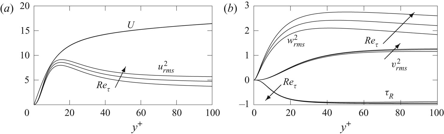
Hitherto it was known but remained unexplained that both in absolute and in relative terms the variation of $u_{rms}^2=\left \langle {u'^2}\right \rangle$ and $w_{rms}^2=\left \langle {w'^2}\right \rangle$ with ${\textit {Re}}_\tau$ is much greater than the variation of $U(y),$ $v_{rms}^2=\left \langle {v'^2}\right \rangle$ and the Reynolds stress $\tau _R=\left \langle {u'v'}\right \rangle$; see figure 2. This figure uses the DNS of a plane channel flow data available at turbulence.oden.utexas.edu. The DNS are described in Hoyas & Jiménez (Reference Hoyas and Jiménez2006) and Lee & Moser (Reference Lee and Moser2015). For the analysis, we fitted the velocity average and its non-zero second moments with explicit expressions. The fit is described in the supplementary material and is available at https://doi.org/10.1017/jfm.2021.180.

Figure 2.

The DNS data for ${\textit {Re}}_\tau =950$, $2000$ and $5200$ showing that $u_{rms}^2$ and $w_{rms}^2$ vary with ${\textit {Re}}_\tau$ significantly more than $U$, $v_{rms}^2$ and $\tau _R=\left \langle {u'v'}\right \rangle$. The three curves for $U$ overlap. Note the difference in the scales of the ordinate axes in the plots.

We introduce the fluctuation of the universal streamwise velocity $\tilde {u}'(\tilde {y})=\tilde {u}(\tilde {y})-\tilde {U}(\tilde {y})$, the universal second moments $\tilde {u}_{rms}^2(\tilde {y})=\left \langle {{{\tilde {u}'\!\,}}^2(\tilde {y})}\right \rangle _{\tilde {y}=\text {const.}}$, $\tilde {v}_{rms}^2(\tilde {y})=\left \langle {\tilde {v}(\tilde {y})^2}\right \rangle _{\tilde {y}=\text {const.}}$, $\tilde {w}_{rms}^2(\tilde {y})=\left \langle {\tilde {w}(\tilde {y})^2}\right \rangle _{\tilde {y}=\text {const.}}$, and the universal mean Reynolds stress $\tilde {\tau }_R(\tilde {y})=\left \langle {\tilde {u}'(\tilde {y})\tilde {v}(\tilde {y})}\right \rangle _{\tilde {y}=\text {const.}}$. Applying the same technique as the technique used to derive (2.20) gives (see appendix A)

(3.1)\begin{align} u_{rms}^2(y)&=\left\langle{(u-U)^2}\right\rangle=\left\langle{\left(u_{\tau_L}\tilde{U}(yu_{\tau_L})\cos\theta\right)^2}\right\rangle-U^2\nonumber\\ &\quad +\left\langle{u_{\tau_L}^2\left(\tilde{u}_{rms}^2(yu_{\tau_L})\cos^2\theta+\tilde{w}_{rms}^2(yu_{\tau_L})\sin^2\theta\right)}\right\rangle, \end{align}

(3.2)\begin{align} v_{rms}^2(y) &=\left\langle{u_{\tau_L}^2\tilde{v}_{rms}^2(yu_{\tau_L})}\right\rangle, \end{align}

(3.3)\begin{align} w_{rms}^2(y) &=\left\langle{w^2(y)}\right\rangle=\left\langle{\left(u_{\tau_L}\tilde{U}(yu_{\tau_L})\sin\theta\right)^2}\right\rangle\nonumber\\ &\quad +\left\langle{u_{\tau_L}^2\left(\tilde{w}_{rms}^2(yu_{\tau_L})\cos^2\theta+ \tilde{u}_{rms}^2(yu_{\tau_L})\sin^2\theta\right)}\right\rangle, \end{align}

(3.4)\begin{align} \left\langle{u'(y)v'(y)}\right\rangle&=\left\langle{u_{\tau_L}^2\tilde{\tau}_R(yu_{\tau_L})\cos\theta}\right\rangle. \end{align}

The Taylor expansions of (3.1)–(3.4) in powers of $\theta$ and $u'_{\tau _L}=u_{\tau _L}-1$ are

(3.5)\begin{gather} u_{rms}^2(y)=\left\langle{u'^2_{\tau_L}}\right\rangle\left(\frac{\displaystyle \textrm{d} y\tilde{U}}{\displaystyle \textrm{d} y}\right)^2+\tilde{u}_{rms}^2(y)+ \frac{\left\langle{u'^2_{\tau_L}}\right\rangle}2 \frac{\displaystyle \textrm{d}^2 y^2\tilde{u}_{rms}^2}{\displaystyle \textrm{d} {y}^2}+ \left\langle{\theta^2}\right\rangle\left(\tilde{w}_{rms}^2-\tilde{u}_{rms}^2\right)+\dots, \end{gather}

(3.6)\begin{gather}v_{rms}^2(y)= \tilde{v}_{rms}^2(y)+\frac12\left\langle{u'^2_{\tau_L}}\right\rangle\frac{\displaystyle \textrm{d}^2 y^2\tilde{v}_{rms}^2}{\displaystyle \textrm{d} {y}^2}+\dots, \end{gather}

(3.7)\begin{gather}w_{rms}^2(y)=\left\langle{\theta^2}\right\rangle\tilde{U}^2+\tilde{w}_{rms}^2(y)+\frac12\left\langle{u'^2_{\tau_L}}\right\rangle\frac{\displaystyle \textrm{d}^2 y^2\tilde{w}_{rms}^2}{\displaystyle \textrm{d} {y}^2}+ \left\langle{\theta^2}\right\rangle\left(\tilde{u}_{rms}^2-\tilde{w}_{rms}^2\right)+\dots, \end{gather}

(3.8)\begin{gather}\left\langle{u'v'}\right\rangle(y) = \tilde{\tau}_R(y)+\frac12\left\langle{u'^2_{\tau_L}}\right\rangle\frac{\displaystyle \textrm{d}^2 y^2\tilde{\tau}_R}{\displaystyle \textrm{d} {y}^2}- \frac{1}{2}\left\langle{\theta^2}\right\rangle\tilde{\tau}_R +\dots . \end{gather}

Note that, for any given $u_{\tau _L}$, negative and positive values of $\theta$ are equally probable (this is a left–right symmetry, similar, for example, to why the average of the fluctuation of the spanwise velocity is zero). Therefore, $\langle u '_{\tau _L}\theta \rangle =0$.

On the right-hand sides of (2.20) and (3.5)–(3.8) only $\left \langle {u'^2_{\tau _L}}\right \rangle$ and $\left \langle {\theta ^2}\right \rangle$ vary with ${\textit {Re}}.$ In (2.20) $\left \langle {u'^2_{\tau _L}}\right \rangle$ and $\left \langle {\theta ^2}\right \rangle$ are multiplied by a factor of the same order of magnitude as $U(y)$ itself. Since variation of $U(y)$ with ${\textit {Re}}$ is very small, the corresponding variation of $\left \langle {u'^2_{\tau _L}}\right \rangle$ and $\left \langle {\theta ^2}\right \rangle$ should also be small. Indeed, for ${\textit {Re}}_\tau$ in the range being considered (between 950 and 5200), the amplitude of large-scale motions is small. For example, for the filter used in Zhang & Chernyshenko (Reference Zhang and Chernyshenko2016), $\left \langle {u'^2_{\tau _L}}\right \rangle = 0.004364$ for ${\textit {Re}}_\tau =1000$, and for the filter used in Zhang (Reference Zhang2019), $\left \langle {u'^2_{\tau _L}}\right \rangle = 0.0031$ for ${\textit {Re}}_\tau =950$ and $\left \langle {u'^2_{\tau _L}}\right \rangle = 0.0064$ for ${\textit {Re}}_\tau =4200$. This allows us to conclude that $\tilde {U}(y)\approx U(y)$, and by the order of magnitude $\tilde {u}_{rms}^2\sim u_{rms}^2$, $\tilde {v}_{rms}^2\sim v_{rms}^2$, $\tilde {w}_{rms}^2\sim w_{rms}^2$, and $\tilde {\tau }_R\sim \left \langle {u'v'}\right \rangle (y)$. Using this for estimating the terms in (2.20) and (3.5)–(3.8) shows that $u_{rms}^2(y)$ and $w_{rms}^2(y)$ stand out. In (3.5) $\left \langle {u'^2_{\tau _L}}\right \rangle$ is multiplied by $({\textrm {d} y}\tilde {U}/{\textrm {d} y})^2$ and in (3.7) $\left \langle {\theta ^2}\right \rangle$ is multiplied by $\tilde {U}^2$. Outside the close vicinity of the wall these factors are large. At $y^+=40$, for example, $({\textrm {d} y}\tilde {U}/{\textrm {d} y})^2\approx 285,$ which is almost 50 times greater than $u^2_{rms}\approx 6$, and $\tilde {U}^2\approx 203,$ which is almost 85 times greater than $w^2_{rms}\approx 2.4.$ There are no such large terms in (2.20), (3.6) and (3.8). The term $\left \langle {u'^2_{\tau _L}}\right \rangle (\textrm {d}{y\tilde {U}}/{\textrm {d} y})^2$ describes the combined action of the amplitude modulation and modulation of the wall-normal length scale of the universal mean profile, which is a QSQH mechanism described in Chernyshenko et al. (Reference Chernyshenko, Marusic and Mathis2012) and Zhang & Chernyshenko (Reference Zhang and Chernyshenko2016). The term $\left \langle {\theta ^2}\right \rangle \tilde {U}^2$ describes the turning of the universal mean profile to follow the fluctuating direction of the large-scale wall friction. Such large terms are not present in the expressions for other quantities. This explains why $u_{rms}^2$ and $w_{rms}^2$ vary more with ${\textit {Re}}$ than $U$, $w_{rms}^2$ and $\left \langle {u'v'}\right \rangle$.

This result allows us to formulate an important observation. The effect of the fluctuation of the direction of the large-scale motion on the statistics of the spanwise velocity is substantial. To confirm these theoretical results, comparisons should be made.

3.2. The profiles of the change in the second moments with ${\textit {Re}}$

The values of $\left \langle {u'^2_{\tau _L}}\right \rangle$ and $\left \langle {\theta ^2}\right \rangle$ and the statistics of the universal velocity depend on the definition of the large-scale filter. Luckily, since $\left \langle {u'^2_{\tau _L}}\right \rangle$ and $\left \langle {\theta ^2}\right \rangle$ are small, $\tilde {U}$ is known quite accurately, and the second moments can be estimated approximately by taking $\tilde {u}_{rms}^2\approx u_{rms}^2$, $\tilde {v}_{rms}^2\approx v_{rms}^2$, $\tilde {w}_{rms}^2\approx w_{rms}^2$ and $\tilde {\tau }_R\approx \left \langle {u'v'}\right \rangle$. Moreover, the dominance of the terms $\left \langle {\theta ^2}\right \rangle \tilde {U}^2$ and $\left \langle {u'^2_{\tau _L}}\right \rangle (\textrm {d}{y\tilde {U}}/{\textrm {d} y})^2$ allows us to express the shape of the increase in $u_{rms}^2$ and $w_{rms}^2$ with ${\textit {Re}}$ as a function of the wall distance in terms of the shape of the mean velocity profile only.

Subtracting (2.22), (3.5)–(3.8) written down for one value of ${\textit {Re}}$ from the same equations for another value of ${\textit {Re}}$ gives the increments of the mean velocity and the second order moments as ${\textit {Re}}$ changes, expressed in terms of the increments of $\left \langle {u'^2_{\tau _L}}\right \rangle$ and $\left \langle {\theta ^2}\right \rangle$,

(3.9)\begin{gather} \Delta U(y)=\frac12\varDelta\left\langle{u'^2_{\tau_L}}\right\rangle \frac{\textrm{d}}{\textrm{d}y} y^2\frac{\displaystyle \textrm{d} \tilde{U}}{\displaystyle \textrm{d} y} - \frac12\varDelta\left\langle{\theta^2}\right\rangle\tilde{U}(y)+\dots, \end{gather}

(3.10)\begin{gather}\Delta u_{rms}^2=\varDelta \left\langle{u'^2_{\tau_L}}\right\rangle\left(\frac{\displaystyle \textrm{d} y\tilde{U}}{\displaystyle \textrm{d} y}\right)^2+\frac12\varDelta \left\langle{u'^2_{\tau_L}}\right\rangle\frac{\displaystyle \textrm{d}^2 y^2\tilde{u}_{rms}^2}{\displaystyle \textrm{d} {y}^2}+ \varDelta \left\langle{\theta^2}\right\rangle\left(\tilde{w}_{rms}^2-\tilde{u}_{rms}^2\right)+\dots, \end{gather}

(3.11)\begin{gather}\Delta v_{rms}^2= \frac{\varDelta\left\langle{u'^2_{\tau_L}}\right\rangle}2\frac{\displaystyle \textrm{d}^2 y^2\tilde{v}_{rms}^2}{\displaystyle \textrm{d} {y}^2}+\dots, \end{gather}

(3.12)\begin{gather}\Delta w_{rms}^2=\frac{\varDelta \left\langle{u'^2_{\tau_L}}\right\rangle}2\frac{\displaystyle \textrm{d}^2 y^2\tilde{w}_{rms}^2}{\displaystyle \textrm{d} {y}^2}+\varDelta \left\langle{\theta^2}\right\rangle\left(\tilde{U}^2+\tilde{u}_{rms}^2-\tilde{w}_{rms}^2\right)+\dots, \end{gather}

(3.13)\begin{gather}\varDelta \left\langle{u'v'}\right\rangle=\frac{\varDelta\left\langle{u'^2_{\tau_L}}\right\rangle}2\frac{\displaystyle \textrm{d}^2 y^2\tilde {\tau}_R}{\displaystyle \textrm{d} {y}^2}-\frac12\left\langle{\theta^2}\right\rangle\tilde{\tau}_R +\dots. \end{gather}

If the terms we identified to be small are dropped, this becomes

(3.14a–c)\begin{equation} \Delta u_{rms}^2\approx\varDelta \left\langle{u'^2_{\tau_L}}\right\rangle\left(\frac{\displaystyle \textrm{d} y\tilde{U}}{\displaystyle \textrm{d} y}\right)^2, \quad \Delta w_{rms}^2\approx \varDelta \left\langle{\theta^2}\right\rangle\tilde{U}^2, \quad \Delta v_{rms}^2\approx \varDelta \left\langle{u'v'}\right\rangle\approx 0. \end{equation}

Comparing the expressions (2.23) for the large-scale components with the expressions for the velocity mean squares (3.1) and (3.3) and their increments (3.10) and (3.12) shows that the non-zero terms in (3.14a–c) are the contributions of the large-scale motion. Thus, (3.14a–c) is in agreement with the well-known observations, see, e.g. Baidya et al. (Reference Baidya, Philip, Hutchins, Monty and Marusic2012), to which (3.14a–c) only adds the form of functional dependence between these increments and the shape of the mean velocity profile.

3.3. Comparisons with numerical simulations and experiment

The prediction of the QSQH theory will be compared with the results of the DNS by Hoyas & Jiménez (Reference Hoyas and Jiménez2006) and Lee & Moser (Reference Lee and Moser2015) and of the experiments by Baidya et al. (Reference Baidya, Philip, Hutchins, Monty and Marusic2012). These results are presented in wall units. All the comparisons will be done for the case of the small amplitude of the fluctuation of large-scale motions: $\left \langle {u'^2_{\tau _L}}\right \rangle \ll 1$ and $\left \langle {\theta ^2}\right \rangle \ll 1$. The relationships that will be verified by comparisons keep only the main term of the expansions in powers of $\left \langle {u'^2_{\tau _L}}\right \rangle$ and $\left \langle {\theta ^2}\right \rangle$. As the relationships (2.8a–c) between the units of the QSQH theory and the wall units show, these units coincide in the main term of the expansion. Moreover, for the values of ${\textit {Re}}_\tau$ considered, the difference between these units is too small to be noticeable in plots. To reflect this, the wall units notation will be used in the plots, but the QSQH notation will be kept in the text.

Some of the comparisons will require the knowledge of the universal mean profile and of the second moments of the universal velocity. From (3.5)–(3.8), it follows that in the main term of the expansion they coincide with the mean and the second moments of the actual velocity. These parameters do not vary significantly within the range of ${\textit {Re}}_\tau$ for which the comparisons will be made, but for consistency we will always use the DNS data for ${\textit {Re}}_\tau =5200$ as describing the universal velocity, that is, we will assume that $(\tilde {U}, \tilde {u}_{rms}^2, \tilde {v}_{rms}^2,\tilde {w}_{rms}^2,\tilde {\tau }_R)=(U,u_{rms}^2, v_{rms}^2,w_{rms}^2, \left \langle {u'v'}\right \rangle )|_{{\textit {Re}}_\tau =5200}$. Each comparison involves two flows at different ${\textit {Re}}_\tau$, which will be specified.

3.3.1. Logarithmic derivatives of the mean square of wall-parallel velocity components

Multiplying by $y$ the logarithmic derivative of (3.14a–c) with respect to $y$ gives

(3.15)\begin{gather} D_u(y)=y\frac{\displaystyle \textrm{d} }{\displaystyle \textrm{d} y}{\ln \Delta u_{rms}^2}\approx 2y\frac{\displaystyle \textrm{d} }{\displaystyle \textrm{d} y}{\ln\frac{\displaystyle \textrm{d} y\tilde{U}}{\displaystyle \textrm{d} y}}, \end{gather}

(3.16)\begin{gather}D_w(y)=y\frac{\displaystyle \textrm{d} }{\displaystyle \textrm{d} y}\ln\Delta w_{rms}^2\approx 2y\frac{\displaystyle \textrm{d} }{\displaystyle \textrm{d} y}\ln\tilde{U}. \end{gather}

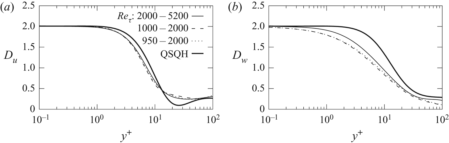
Figure 3 shows the comparison for $D_u$ and $D_w$. Figure 3(a) is effectively the same as figure 12 in Zhang & Chernyshenko (Reference Zhang and Chernyshenko2016), with the curve corresponding to the increment in ${\textit {Re}}_\tau$ from 950 to 2000 added, and the quality of the DNS data fit improved, in particular in the area of small values of $y^+$. It is worth mentioning that since the value of the $y$-multiplied logarithmic derivative of any function proportional to ${y}^2$ as $y\to 0$ is 2, the very good agreement for very small values of $y$ should not be overrated. In figure 3(b) close to $y^+=100$ the deviation of the curves for the differences between the flows with ${\textit {Re}}_\tau$ of 950 and 2000 and of 1000 and 2000 is due to the imperfection of the functional fit to the DNS data, aggravated by differentiation. Figure 3(b) shows that the agreement between DNS and the QSQH theory noticeably improves as ${\textit {Re}}_\tau$ increases. This is expected, but figure 3(b) is the first definite confirmation that the accuracy of the three-dimensional QSQH hypothesis improves with increasing ${\textit {Re}}_\tau$. The improvement can also be noticed in figure 3(a), although in that figure the agreement is noticeably better, while the improvement is smaller.

Figure 3.

Comparison of the logarithmic derivatives of the increments of $u_{rms}^2$ (a) and $w_{rms}^2$ (b) as ${\textit {Re}}_\tau$ varies. Thin curves are DNS results. The QSQH predictions are (3.15) and (3.16). The increments correspond to the changes in ${\textit {Re}}_\tau$ as shown.

Comparison using logarithmic derivatives cannot be extended to the full formulae (3.9)–(3.13). Fortunately, it is still possible to compare if not the magnitude but at least the shape of the curves of the increments of the second moments themselves rather than their derivatives. To do this, we fit $\Delta u_{rms}^2(y)$ and $\Delta w_{rms}^2(y)$ with the expressions (3.15) and (3.16), using $\varDelta \left \langle {u'^2_{\tau _L}}\right \rangle$ and $\varDelta \left \langle {\theta ^2}\right \rangle$ as the fitting parameters. Fitting was done with the gnuplot command ‘fit’, which implements the nonlinear least-squares Marquardt–Levenberg algorithm. 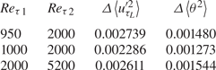The obtained values of $\varDelta \left \langle {u'^2_{\tau _L}}\right \rangle$ and $\varDelta \left \langle {\theta ^2}\right \rangle$ are listed in table 1. 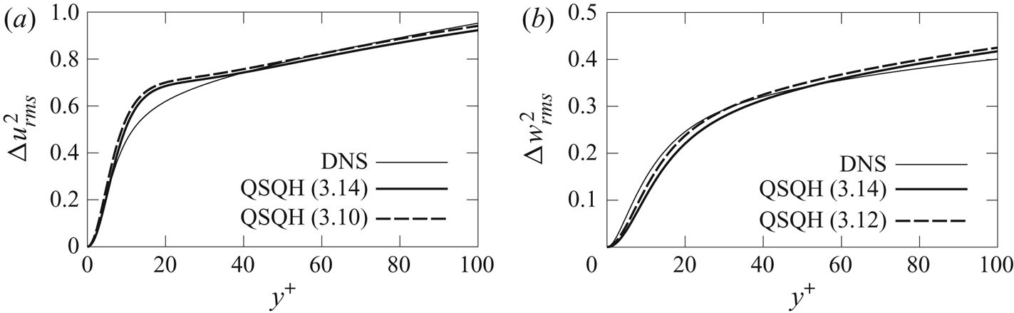With these values, $\Delta u_{rms}^2(y)$ and $\Delta w_{rms}^2(y)$ can be found not only from (3.14a–c) but also from (3.10), (3.12). Both results are shown in figure 4. Overall, the deviation of the QSQH predictions for $\Delta u_{rms}^2$ and $\Delta w_{rms}^2$ is not large and is of the same order of magnitude as reported in most cases in Zhang & Chernyshenko (Reference Zhang and Chernyshenko2016). This further confirms that near the wall the variation of $u_{rms}^2$ and $w_{rms}^2$ with ${\textit {Re}}$ is dominated by the QSQH mechanism. It is interesting to note that while figures 3 and 4 are comparisons for the same QSQH formulae, the visual impression is that in figure 3 the predictions involving $\Delta u_{rms}^2$ are more accurate than the prediction involving $\Delta w_{rms}^2$ while vice versa in figure 4.

Table 1.

Increments of $\left \langle {u'^2_{\tau _L}}\right \rangle$ and $\left \langle {\theta ^2}\right \rangle$ as ${\textit {Re}}_\tau$ grows from ${{\textit {Re}}_\tau }_1$ to ${{\textit {Re}}_\tau }_2$, fitted to (3.14a–c). Four digits are accurate only for the specific fits to the specific set of data as described in the text.

Figure 4.

Comparison of the increments of $u_{rms}^2$ and $w_{rms}^2$ as ${\textit {Re}}_\tau$ changes from 2000 to 5200. The thin curves are DNS results. The solid curves are QSQH predictions with simplified formulae (3.14a–c) and the dashed curves are QSQH predictions with the full formulae (3.10) and (3.12). The fitting parameters $\varDelta \left \langle {u'^2_{\tau _L}}\right \rangle$ and $\varDelta \left \langle {u'^2_{\tau _L}}\right \rangle$ are given in table 1.

The small difference between the QSQH predictions for $\Delta u_{rms}^2$ and $\Delta w_{rms}^2$ obtained using (3.14a–c) and (3.10), (3.12) confirms that the terms dropped in (3.14a–c) are small.

The use of fitting has a drawback. The QSQH theory relies on the assumption that there exists a large-scale filter satisfying the properties P1–P5 (2.1)–(2.5). The good agreement in figure 4 does not guarantee with full certainty however that the values of $\varDelta \left \langle {u'^2_{\tau _L}}\right \rangle$ and $\varDelta \left \langle {\theta ^2}\right \rangle$ obtained with such a filter and the values obtained by fitting are close. The comparisons in figure 3 are free from this complication because, with $\tilde {U}\approx U$, (3.15) and (3.16) establish a flow property that is independent of the definition or even existence of the large-scale filter. Another informative comparison of such nature can be done by introducing functions $R_u(y)$ and $R_w(y)$ as

(3.17a,b)\begin{equation} R_u(y)=\frac{\Delta u_{rms}^2}{\left(\frac{\displaystyle \textrm{d} y\tilde{U}}{\displaystyle \textrm{d} y}\right)^2\left(1+C_u(y)\right)}, \quad R_w(y)=\frac{\Delta w_{rms}^2}{U^2\left(1+C_w(y)\right)}, \end{equation}

where

(3.18)\begin{equation} C_u(y)=\left.\left(\frac12\frac{\displaystyle \textrm{d}^2 y^2\tilde{u}_{rms}^2}{\displaystyle \textrm{d} {y}^2}+ \frac{ \varDelta \left\langle{\theta^2}\right\rangle }{ \varDelta \left\langle{u'^2_{\tau_L}}\right\rangle} \left( \tilde{w}_{rms}^2-\tilde{u}_{rms}^2\right)+\dots \right) \right/\left( \frac{\displaystyle \textrm{d} y\tilde{U}}{\displaystyle \textrm{d} y} \right)^2 , \end{equation}

and

(3.19)\begin{equation} C_w(y) = \left.\left(\frac{\varDelta \left\langle{u'^2_{\tau_L}}\right\rangle}{2\varDelta \left\langle{\theta^2}\right\rangle}\frac{\displaystyle \textrm{d}^2 y^2\tilde{w}_{rms}^2}{\displaystyle \textrm{d} {y}^2}+\tilde{u}_{rms}^2- \tilde{w}_{rms}^2\right)\right/ U^2+\dots. \end{equation}

Then (3.10) and (3.12) state that $R_u(y)=\varDelta \left \langle {u'^2_{\tau _L}}\right \rangle$ and $R_w(y)=\varDelta \left \langle {\theta ^2}\right \rangle$. The same follows from (3.14a–c) with the additional assumption that $C(y)_u=C_w(y)=0$. In fact, $C_u(y)$ and $C_w(y)$ are just the ratios of the terms neglected to the terms kept when (3.14a–c) was obtained from (3.10) and (3.12). Therefore, the QSQH theory predicts that, for the small amplitude of the fluctuation of the large-scale motions, functions $R_u(y)$ and $R_w$(y) are independent of $y$. Moreover, with $C_u$ and $C_w$ neglected, these functions do not depend on the large-scale filter or any other elements of the QSQH theory: this is a prediction about the properties of the flow itself.

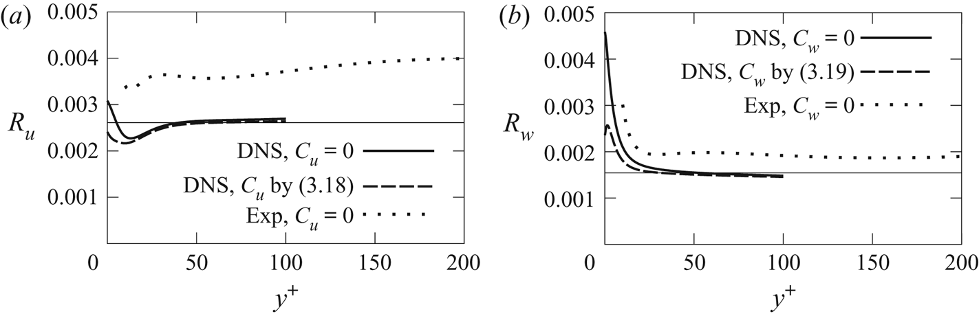
Plots of $R_u(y)$ and $R_w(y)$ are shown in figure 5. The DNS data are for the difference of the mean velocity squares in flows in a plane channel with ${\textit {Re}}_\tau =2000$ and $5200$. The data range up to 100 wall units is determined by the range of our fits to the mean square velocities, which in turn was selected on the basis of previous findings (Zhang & Chernyshenko Reference Zhang and Chernyshenko2016; Agostini & Leschziner Reference Agostini and Leschziner2019b) that at least for ${\textit {Re}}_\tau =1000$ the QSQH predictions deviate from the DNS results for $y^+>100$. The experimental data are for a zero pressure gradient boundary layer with ${\textit {Re}}_\tau =3000$ and 10 500 (Baidya et al. Reference Baidya, Philip, Hutchins, Monty and Marusic2012). For these higher ${\textit {Re}}_\tau$, the comparison data range was extended to $y^+=200$. The data were obtained by digitizing the large-scale contribution points in figure 5 in Baidya et al. (Reference Baidya, Philip, Hutchins, Monty and Marusic2012), and then using the same curve-fitting procedure as described in the supplement for the DNS data. The large-scale contribution was used because the variation of the small-scale contribution is small, as evidenced by that figure itself, and as predicted by the QSQH theory, and because the comparison was made only for $C_u=C_w=0$, that is, for the QSQH predictions for the large-scale contribution (see the discussion following (3.14a–c)). The curves are flat for larger values of $y^+$, which corresponds to the QSQH prediction, but, predictably, have noticeable variation near the wall, where $C_u$ and $C_w$ are not negligible. Figures 3–5 are various ways of verifying the same predictions (3.10), (3.12) and (3.14a–c). The seeming discrepancy in the performance of the QSQH theory is due to these figures describing different measures of the error. Thus, near the wall figure 3 effectively compares the exponent of $y^+$ of the $y^+\to 0$ asymptotics of (3.10), (3.12) and (3.14a–c), figure 4 compares the absolute error, and figure 5 effectively compares the relative error. Fortunately, comparisons for the other two moments, $v_{rms}^2$ and $\left \langle {u'v'}\right \rangle$, give further insight into the physics of the question.

Figure 5.

Comparison of the functions $R_u(y^+)$ and $R_w(y^+)$, (3.17a,b), with DNS and experimental data. In the limit of the small amplitude of the fluctuation of the large-scale motions the QSQH theory predicts that $R_u$ and $R_w$ are independent of $y^+$. The DNS results are for channel flows with ${\textit {Re}}_\tau$ changing from 2000 to 5200, and the experimental results are for a boundary layer with ${\textit {Re}}_\tau$ changing from 3000 to 10 500. The solid and dotted curves are for $C_u=C_w=0$. The dashed curves use the full formulae (3.18) and (3.19). The horizontal straight lines are the values of $\varDelta \left \langle {u'^2_{\tau _L}}\right \rangle$ and $\varDelta \left \langle {\theta ^2}\right \rangle$ from table 1.

The large-scale motions contribute to $\Delta v_{rms}^2$ and $\varDelta \left \langle {u'v'}\right \rangle$ only indirectly by modifying the small-scale structures. If this effect is neglected, as in (3.14a–c), the predicted increments of $\Delta v_{rms}^2$ and $\varDelta \left \langle {u'v'}\right \rangle$ are zero. Accordingly, the comparisons for these quantities are made only for the full predictions. 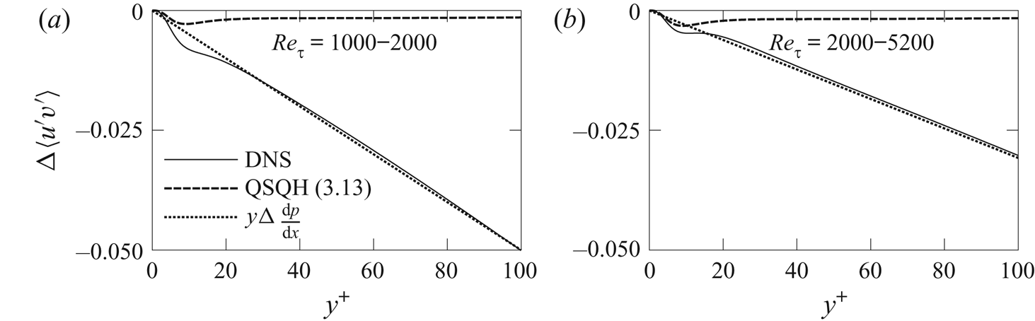The QSQH predictions for $\varDelta \left \langle {u'v'}\right \rangle$ deviate considerably, by an order of magnitude, from the DNS results, as shown in figure 6. The almost linear behaviour of $\varDelta \left \langle {u'v'}\right \rangle$ for $y^+>20$ suggests an explanation. It is well known that the dependence of the total shear stress on the distance to the channel wall is linear and in wall units is equal to $y^+\textrm {d}p^+/{\textrm {d} x}^+=y^+/{\textit {Re}}_\tau ,$ and that further away from the wall the Reynolds stress approaches the total stress. The corresponding change in the total stress, equal to $y^+\Delta \textrm {d}p^+{\textrm {d}x}^+=y^+(1/{\textit {Re}}_{\tau _2}-1/{\textit {Re}}_{\tau _1}),$ is shown with a dotted line. It closely agrees with the DNS result everywhere except the vicinity of the wall, where both the QSQH effect and the pressure gradient effect are of the same order of magnitude. As ${\textit {Re}}_\tau$ changes, so does the pressure gradient. Comparing the curves for different ${\textit {Re}}_\tau$ in figure 6 suggests that QSQH modulation effects can become more significant than the effect of the pressure gradient only at much higher ${\textit {Re}}_\tau$.

Figure 6.

Comparison of the increments of $\left \langle {u'v'}\right \rangle$ as ${\textit {Re}}_\tau$ changes from 1000 to 2000 (a) and from 2000 to 5200 (b). Thin curves are DNS results. The QSQH predictions are (3.13), shown with dashed curves. The dotted curve is $y^+\Delta \textrm {d}p^+/{\textrm {d} x}^+.$ The fitting parameters $\varDelta \left \langle {u'^2_{\tau _L}}\right \rangle$ and $\varDelta \left \langle {u'^2_{\tau _L}}\right \rangle$ are given in table 1.

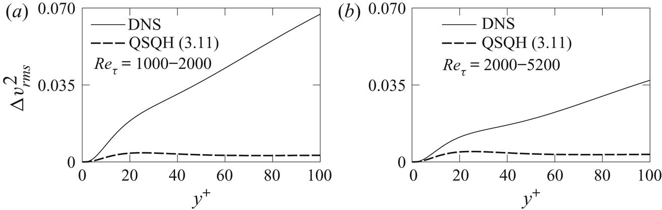
Comparisons made in figure 7 for $\Delta v_{rms}^2$ also reveal a significant deviation of the QSQH predictions from the DNS results. There is no simple formula for the quantitative description of the effect of the pressure gradient on $v_{rms}$, but since both $v_{rms}$ and $\left \langle {u'v'}\right \rangle$ depend on the properties of the wall-normal velocity, it is reasonable to assume that their similar behaviour has the same nature. This is further confirmed by the decrease of the deviation as ${\textit {Re}}_\tau$ increases.

Figure 7.

Comparison of the increments of $v_{rms}^2$ as ${\textit {Re}}_\tau$ changes from 1000 to 2000 (a) and from 2000 to 5200 (b). Thin curves are DNS results. The QSQH predictions are (3.11). The fitting parameters $\varDelta \left \langle {u'^2_{\tau _L}}\right \rangle$ and $\varDelta \left \langle {u'^2_{\tau _L}}\right \rangle$ are given in table 1.

The comparisons in the section draw a clear physical picture. The near-wall turbulent flows are affected both by the large-scale structures and other effects, unrelated to large-scale structures, such as the pressure gradient in a channel flow. In the range of the ${\textit {Re}}_\tau$ considered, that is, primarily from $1000$ to $5000$, these mechanisms can create effects of various magnitude depending on the particular statistic in question and the distance to the wall. When the effect of the large-scale structures dominates, it can be described by the QSQH theory.