1. Introduction
Shock waves are very common in systems that involve fluid flows. Such systems occur on very different scales – from the microphysical scale to the astronomical scale. As such, the properties of such shocks can vary considerably, depending on the environment. From the microphysical point of view, it is useful to discriminate between collisional and collisionless shocks. Collisional shock waves, first discovered in the nineteenth century (Salas Reference Salas2007), can occur in any fluid as the result of a steepening of a large-amplitude sound wave, or collision of two media (Zel'dovich & Raizer Reference Zel'dovich and Raizer2002). The front of a collisional shock is necessarily at least a few mean-free-paths thick, as the dissipation from the downstream to the upstream occurs via binary collisions.
Collisionless shock waves were discovered later and can only form in plasma (Petschek Reference Petschek1958; Buneman Reference Buneman1964; Sagdeev Reference Sagdeev1966). The dissipation is provided by collective plasma phenomena instead of binary collisions. As a result, the front of such shocks can be orders of magnitude thinner than the mean free path. For example, the front of the bow shock of Earth's magnetosphere in the solar wind is some 100 km thick (Bale, Mozer & Horbury Reference Bale, Mozer and Horbury2003; Schwartz et al. Reference Schwartz, Henley, Mitchell and Krasnoselskikh2011). Yet, the proton mean free path at this location is about the Sun–Earth distance, nearly seven orders of magnitude greater. Hence, if the Earth bow shock were collisional, its front would be about 1 a.u. thick (see also § 2.1.3 of Balogh & Treumann (Reference Balogh and Treumann2013) and references therein).
Is it possible to bridge between these two regimes? How does a shock switch from a regime where its front is a few mean-free-paths thick to another regime where its front is a million times smaller? Exploring the intermediate case, bridging between collisional and collisionless shocks, is the aim of this article.
On the collisionless side, shock-accelerated particles which can enhance the density jump, or external magnetization which can reduce it, will be ignored (Berezhko & Ellison Reference Berezhko and Ellison1999; Bret & Narayan Reference Bret and Narayan2018, Reference Bret and Narayan2019; Bret Reference Bret2020).
The method implemented is explained in § 2. The overall picture is as follows: we first present an evaluation of the shock front thickness in the collisional regime, then in the collisionless regime. The first task is achieved in § 3 using the Mott-Smith ansatz (Mott-Smith Reference Mott-Smith1951), which expresses the distribution function at any place along the shock profile as a linear combination of the upstream and downstream Maxwellians. We then follow Tidman (Reference Tidman1967) in § 4 for the collisionless case before we bridge between the two expressions of the front thickness in § 5, to propose an expression of the front thickness valid from the collisional to the collisionless regime.
2. Method
As previously stated, a fluid shock is mediated by collisions while a collisionless shock is mediated by collective effects. For a plasma where only electrostatic fields are active (such is the case for an electrostatic shock), the kinetic equation accounting for both kinds of effects would formally read (Kulsrud Reference Kulsrud2005, p. 9)
 \begin{equation} \frac{\partial F}{\partial t} + \boldsymbol{v} \boldsymbol{\cdot} \frac{\partial F}{\partial \boldsymbol{r}} + \frac{q \boldsymbol{E}}{m}\boldsymbol{\cdot}\frac{\partial F}{\partial \boldsymbol{v}} = \left( \frac{\partial F}{\partial t}\right)_c + \left( \frac{\partial F}{\partial t}\right)_w, \end{equation}
where  $q$ and
 $m$ are the charge and the mass of the species considered. The first term on the right-hand side, namely
 $(\partial F/\partial t)_c$, represents the rate of change of the distribution
 $F$ due to collisions. It is typically given by the Fokker–Planck operator. The second term,
 $(\partial F/\partial t)_w$, accounts for the effects of the waves and is given, for example, by the quasi-linear operator. In principle, accounting at once for these two collision terms with appropriate collision operators should allow a description of a shock wave from the collisional regime to the fully collisionless regime.
Resolving the shock front requires a formalism capable of resolving the entire shock profile. This is a notoriously difficult problem which has been greatly aided by the introduction of the so-called Mott-Smith ansatz (Mott-Smith Reference Mott-Smith1951). Initially introduced for a neutral fluid, this ansatz consists of approximating the molecular distribution function  $F$ along the shock profile by a linear combination of the upstream and downstream drifting Maxwellians:
 \begin{align} F(\boldsymbol{v}) &= n_1(x)\left(\frac{m}{2{\rm \pi} k_BT_1}\right)^{3/2}\exp\left(-\frac{m}{2 k_BT_1}(\boldsymbol{v}-\boldsymbol{U}_1)^2\right) \nonumber\\ &\quad + n_2(x)\left(\frac{m}{2{\rm \pi} k_BT_2}\right)^{3/2}\exp\left(-\frac{m}{2 k_BT_2}(\boldsymbol{v}-\boldsymbol{U}_2)^2\right), \end{align}
where  $T_{1,2}$ and
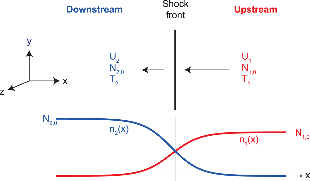
 $\boldsymbol {U}_{1,2}$ are the upstream (subscript 1) and downstream (subscript 2) temperatures and velocities, respectively, determined by the Rankine–Hugoniot (RH) jump conditions (see figure 1).Footnote 1 The boundary conditions for the functions
 $n_{1,2}(x)$ are
 \begin{equation} \left. \begin{array}{c@{}} n_1(+\infty) = N_{1,0} \quad n_1(-\infty) = 0, \\ n_2(+\infty) = 0 \quad n_2(-\infty) = N_{2,0} , \end{array}\right\} \end{equation}
where again  $N_{1,0}$ and
 $N_{2,0}$ fulfil the RH jump conditions.
Set-up and notations.

Taking then the appropriate moments of the dispersion equation gives a differential equation which allows the determination of the respective weights of the two Maxwellians in terms of  $x$, and hence the shock profile together with its front thickness (Mott-Smith Reference Mott-Smith1951).
The method implemented here consists of dealing with the collisional and the collisionless regimes separately.
• We study the collisional regime in § 3. There we apply the Mott-Smith ansatz using the BGK collision term (Bhatnagar, Gross & Krook Reference Bhatnagar, Gross and Krook1954) as a collision operator for
 $(\partial F/\partial t)_c$ in (2.1), with $(\partial F/\partial t)_w=0$. Notably, Bhatnagar et al. (Reference Bhatnagar, Gross and Krook1954) presented four different collision operators through their (3), (4), (5)–(6), (15)–(19). Those given by (3), (4), (5)–(6), like $\nu (f-f_0)$,Footnote 2 have been widely used although they do not conserve all three quantities: particle number and/or momentum and/or energy. In Bhatnagar et al. (Reference Bhatnagar, Gross and Krook1954), only the operator of (15)–(19) does conserve all three, and hence this is the one used here.
Tidman (Reference Tidman1958) used the Fokker–Planck operator to deal with the problem, considering (2.1) with
$(\partial F/\partial t)_w=0$ and
(2.4)where\begin{equation} \left( \frac{\partial F}{\partial t}\right)_c = \frac{4{\rm \pi} e^4}{m_i^2} \ln \varLambda \left( \frac{\partial F}{\partial t}\right)_{c,\textrm{FP}}, \end{equation}$(\partial F/\partial t)_{c,\textrm {FP}}$ is the Fokker–Planck collision operator, $m_i$ the ion mass and $\varLambda$ the number of particles in the Debye sphere, that is, the co-called ‘plasma parameter’ which measures the coupling of the plasma. As we shall see in § 6, the present treatment provides a more adequate bridging to the collisionless regime than Reference TidmanTidman's (Reference Tidman1958) Fokker–Planck result.• For the collisionless regime we follow in § 4 the collisionless result of Tidman (Reference Tidman1967) who also used the Mott-Smith ansatz. In recent years, the correctness of this approximation, namely that the distribution function is well approximated by superimposed drifting Maxwellians, was validated numerically using particle-in-cell simulations (Spitkovsky Reference Spitkovsky2008). Tidman (Reference Tidman1967) considered (2.1) with
$(\partial F/\partial t)_c=0$, describing $(\partial F/\partial t)_w=0$ by the quasi-linear operator.


Having assessed the width of the shock front in the collisional and the collisionless regimes, we then bridge between the two expressions of the shock thickness in § 5.
3. Collisional regime: applying the BGK collision term to the Mott-Smith ansatz
We switch to the reference frame of the shock and assume steady state in this frame. As in Tidman (Reference Tidman1958), we consider the distributions are functions of  $(v_x,v_y,v_z)$ and assume quantities only vary with the
 $x$ coordinate. We therefore set
 $\partial _{y,z,t}=0$ and
 $E_{y,z}=0$ so that (2.1), with
 $(\partial F/\partial t)_w=0$, reads for the ion distribution
 $F$ as
 \begin{equation} v_x\frac{\partial F}{\partial x } + \frac{e E_x}{m_i}\frac{\partial F}{\partial v_x } = \left( \frac{\partial F}{\partial t }\right)_{c,\textrm{BGK}}, \end{equation}
where  $m_i$ is the ion mass. The BGK collision term now reads (Bhatnagar et al. Reference Bhatnagar, Gross and Krook1954; Gross & Krook Reference Gross and Krook1956)
 \begin{equation} \left( \frac{\partial F}{\partial t }\right)_{c,\textrm{BGK}} = \frac{1}{\sigma}( N^2 \varPhi-N F ), \end{equation}
which vanishes for a Maxwellian distribution. According to Bhatnagar et al. (Reference Bhatnagar, Gross and Krook1954), ‘ $\sigma ^{-1} \times$ a density’ is a collision frequency
 $\nu$. In the present setting we define
 \begin{equation} \frac{N_{1,0}}{\sigma} = \nu \sim \frac{v_{\mathrm{thi},1}}{\lambda_{\mathrm{mfp},1}} \Rightarrow \sigma = \frac{N_{1,0} \lambda_{\mathrm{mfp},1}}{v_{\mathrm{thi},1}} , \end{equation}
where  $v_{\mathrm {thi},1}$ and
 $\lambda _{\mathrm {mfp},1}$ are the upstream thermal velocity and mean free path, respectively. Then
 $N$ and
 $\varPhi$ are given by (15)–(19) of Bhatnagar et al. (Reference Bhatnagar, Gross and Krook1954):
 \begin{gather} N = \int F \, \textrm{d}^3v =n_1 (x) + n_2(x), \end{gather}
 \begin{gather}\varPhi = \left( \frac{m_i}{2{\rm \pi} k_BT } \right)^{3/2}\exp\left( -\frac{m_i}{2 k_BT }(\boldsymbol{v}-\boldsymbol{q} )^2 \right), \end{gather}
 \begin{gather}\boldsymbol{q} = \frac{1}{N}\int \boldsymbol{v} F \, \textrm{d}^3v, \end{gather}
 \begin{gather}\frac{3 k_BT }{m_i} = \frac{1}{N}\int (\boldsymbol{v}-\boldsymbol{q} )^2 F \, \textrm{d}^3v, \end{gather}
where  $F$ has been considered of the form (2.2). Multiplying (3.1) by
 $v_y^2$ and integrating over
 $\textrm {d}^3v$ (see detailed calculation reported in Appendix A) gives an exact, simple result:
 \begin{equation} U_1\frac{k_BT_1}{m_i} \frac{\partial n_1}{\partial x} + U_2\frac{k_BT_2}{m_i} \frac{\partial n_2}{\partial x} = \frac{1}{3\sigma } (U_1-U_2 )^2 n_1 n_2. \end{equation}
This differential equation is structurally identical to the ones found in Mott-Smith (Reference Mott-Smith1951) and Tidman (Reference Tidman1958). We show in Appendix B how it yields density profiles like the ones pictured in figure 1, of the form
 \begin{gather} n_1(x) = N_{1,0} \frac{1}{1+e^{{-}x/\ell}}, \end{gather}
 \begin{gather}n_2(x) = N_{2,0} \frac{e^{{-}x/\ell}}{1+e^{{-}x/\ell}}, \end{gather}
implicitly defining the shock width  $\ell$. From (B 7) we find the thickness of the shock according to the present formalism:
 \begin{equation} \ell=3\sigma \frac{ k_B(T_1 - T_2) U_2 }{ N_{1,0} m_i (U_1-U_2)^2} = 3 \frac{N_{1,0} \lambda_{\mathrm{mfp},1}}{v_{\mathrm{thi},1}} \frac{ k_B(T_1 - T_2) U_2 }{ N_{1,0} m_i (U_1-U_2)^2}. \end{equation}
It is now convenient to use the RH jump conditions to express  $\ell$ in terms of the upstream quantities, like the upstream Mach number and mean free path. The calculations reported in Appendix C give
 \begin{align} \ell &= \lambda_{\mathrm{mfp},1}\frac{U_1}{v_{\mathrm{thi},1}} \frac{ (\mathcal{M}_1^2+3 ) (5 \mathcal{M}_1^2 (\mathcal{M}_1^2+2 )-3 )}{5 \mathcal{M}_1^2 (\mathcal{M}_1^2-1)^2} \nonumber\\ &= \lambda_{\mathrm{mfp},1} \frac{ (\mathcal{M}_1^2+3 ) (5 \mathcal{M}_1^2 (\mathcal{M}_1^2+2 )-3 )}{5 \mathcal{M}_1 (\mathcal{M}_1^2-1)^2}, \end{align}
where  $\mathcal {M}_1$ is the upstream Mach number.Footnote 3 We eventually obtain the following limits for the shock width
 $\ell$:
 \begin{equation} \ell = \lambda_{\mathrm{mfp},1} \times \left\{\begin{array}{@{}ll} \dfrac{12}{5}(\mathcal{M}_1-1)^{{-}2} & \mathrm{for}\ \mathcal{M}_1 \sim 1, \\ \mathcal{M}_1 & \mathrm{for}\ \mathcal{M}_1 \rightarrow \infty. \end{array} \right. \end{equation}
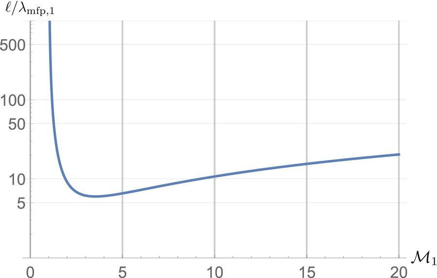
The function  $\ell /\lambda _{\mathrm {mfp},1}$ is plotted in figure 2 in terms of the Mach number. It reaches a minimum for
 $\mathcal {M}_1=3.53$ with
 $\ell /\lambda _{\mathrm {mfp},1}=6$. Such a ‘U’ shape has also been found in Tidman (Reference Tidman1958). We shall further comment on Tidman (Reference Tidman1958) in § 6.
Shock front thickness in units of the mean free path,  $\ell /\lambda _{\mathrm {mfp},1}$, in terms of the upstream Mach number
 $\mathcal {M}_1$.

4. Collisionless regime
Our expression (3.13) for the shock width cannot be used to bridge all the way to collisionless shocks since it has been derived from the kinetic (2.1) without the  $(\partial F/\partial t)_w$ collision term. Yet, collisionless shocks are sustained by the mechanism described by this very term. Tidman (Reference Tidman1967) treated the problem of a collisionless shock by setting
 $(\partial F/\partial t)_c=0$ in (2.1) and considering the quasi-linear operator for
 $(\partial F/\partial t)_w$. The Mott-Smith ansatz was also implemented in this study. Tidman (Reference Tidman1967) could not derive an equation of the form (3.8) allowing an extraction of an analytical shock profile. Further analysis in Biskamp & Pfirsch (Reference Biskamp and Pfirsch1969) and Tidman & Krall (Reference Tidman and Krall1969) concluded that the quasi-linear formalism is not nonlinear enough to fully render a shock.
Yet, Tidman (Reference Tidman1967) could derive the following estimate of the width of the front:
 \begin{align} \ell &= A\frac{U_1}{\omega_{pi,1}} = A \frac{U_1}{v_{\mathrm{thi},1}} \frac{v_{\mathrm{thi},1}}{\omega_{\textrm{pi},1}} \nonumber\\ &= A \mathcal{M}_1 \lambda_{\mathrm{Di},1}, \end{align}
where  $\lambda _{\mathrm {Di},1}$ is the upstream ionic Debye length and
 $A$ is a parameter expected to be of
 ${O}(10)$. We can eventually cast this result in the form
 \begin{equation} \ell = A \mathcal{M}_1 \frac{\ln \varLambda}{\varLambda} \lambda_{\mathrm{mfp,1}}, \end{equation}
where  $\varLambda$ is the plasma parameter already introduced in (2.4) and we have used (Fitzpatrick Reference Fitzpatrick2014, p. 10)
 \begin{equation} \lambda_{\mathrm{mfp,1}} = \frac{\varLambda}{\ln \varLambda}\lambda_{\mathrm{Di},1}. \end{equation}
Notably, Tidman (Reference Tidman1967) only addressed high-Mach-number turbulent shocks triggered by electrostatic instabilities. The forthcoming bridging between the two regimes is therefore only valid for such shocks. Weibel shocks sustained by electromagnetic instabilities are therefore excluded (Stockem et al. Reference Stockem, Fiuza, Bret, Fonseca and Silva2014; Ruyer et al. Reference Ruyer, Gremillet, Bonnaud and Riconda2017).
5. Bridging between the two regimes
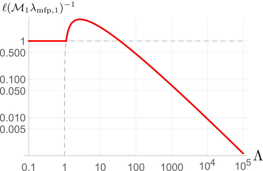
Figure 3 shows the collisional and collisionless expressions of  $\ell (\mathcal {M}_1 \lambda _{\mathrm {mfp},1})^{-1}$ from (3.13) and (4.2). For upstream Mach number
 $\mathcal {M}_1$ greater than a few (4–5), these two expressions intersect for a critical plasma parameter
 $\varLambda _c$ defined by
 \begin{equation} \lambda_{\mathrm{mfp},1} \mathcal{M}_1 = A \mathcal{M}_1 \frac{\ln \varLambda_c}{\varLambda_c} \lambda_{\mathrm{mfp,1}} \Rightarrow 1 = A \frac{\ln \varLambda_c}{\varLambda_c}, \end{equation}
fulfilled for  $\varLambda _c \sim 1.12$ and then for
 $\varLambda _c \sim 35$ (for
 $A=10$).
Plot of  $\ell (\mathcal {M}_1 \lambda _{\mathrm {mfp},1})^{-1}$ in terms of
 $\varLambda$. For a collisional plasma with small
 $\varLambda$, the front thickness
 $\ell$ is given by (3.13). The collisionless thickness is given by (4.2). The width of the front for any plasma parameter
 $\varLambda$ is given by the red curve. Only valid for strong shock (see the final discussion of § 4).

For  $\varLambda < 1.12$, the upstream is strongly coupled, that is, collisional, and the width of the front will be given by the collisional result (3.13). For
 $\varLambda > 1.12$, the upstream is weakly coupled, that is, collisionless, and the relevant front width is therefore the collisionless result (4.2). Hence, the larger value of
 $\varLambda _c \sim 35$ where the two expressions intersect again is not physically meaningful. For such values of
 $\varLambda$, the upstream is collisionless so that the collisionless result applies.
The transition between the two regimes occurs therefore for a critical plasma parameter  $\varLambda _c = 1.12$, coinciding with the transition of the upstream from the strongly coupled/collisional regime to the weakly coupled/collisionless regime. Although this value of
 $\varLambda _c$ has been computed for
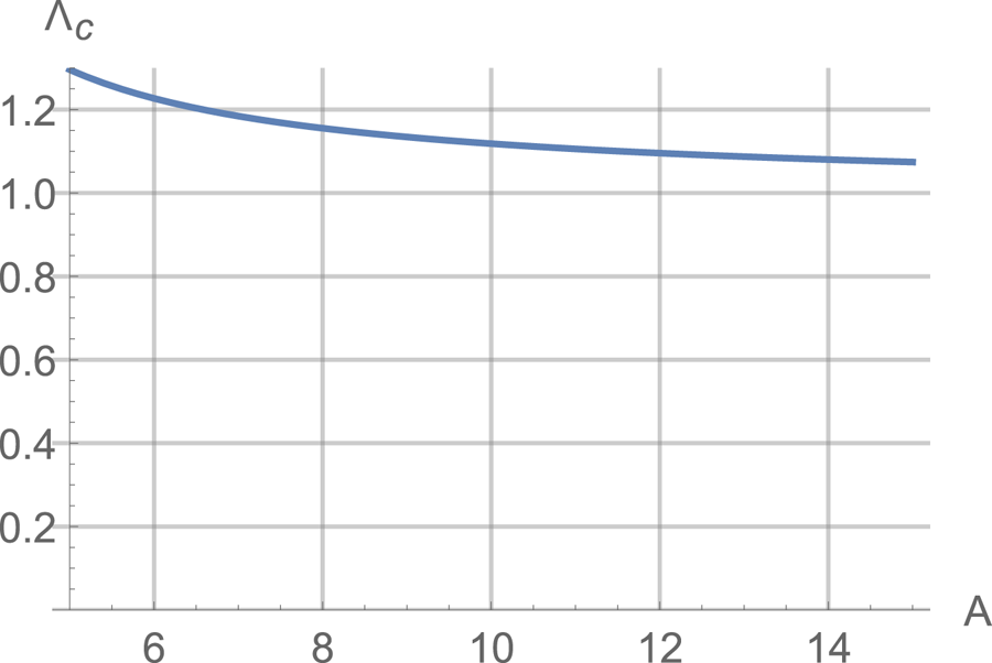
 $A=10$, figure 4 shows that it is poorly sensitive to
 $A$ as long as
 $A={O}(10)$.


Note that this value of  $\varLambda _c = 1.12$ is only indicative. For example, Lee & More (Reference Lee and More1984) developed an electron conductivity model for dense plasmas requiring
 $\ln \varLambda \geq 2$, i.e.
 $\varLambda \geq e^2=7.39$. Therefore, while
 $\varLambda =35$ probably pertains to weakly collisional plasmas, the value
 $\varLambda _c = 1.12$ only gives a general idea of where the transition occurs.
The width of the front for any plasma parameter  $\varLambda$ is eventually given by the red curve in figure 3. Simply put, the nature of the shock is the same as the nature of the upstream. Both are collisional or collisionless together.
The non-monotonic behaviour in the collisionless regime is just a consequence of the non-monotonic variation of the mean free path in terms of the plasma parameter. The function  $g(x)=A\ln x/x$ reaches a maximum for
 $x=e$ with
 $g(e)=3.67$, still for
 $A=10$.
6. Comparison with Tidman (Reference Tidman1958)
A calculation parallel to the one performed in § 3 for the collisional regime was achieved in Tidman (Reference Tidman1958). However, as we show here, the bridging it provides to the collisionless regime is inadequate.
For the ion distribution function  $F$, Tidman (Reference Tidman1958) used the Fokker–Planck operator for
 $(\partial F/\partial t)_c$ in (2.1), set
 $(\partial F/\partial t)_w=0$ and found for strong shocks thatFootnote 4
 \begin{equation} \ell_T = \alpha \frac{c_s^4}{N_{1,0}\varGamma}\mathcal{M}_1^4, \end{equation}
where  $\alpha =29.1/512{\rm \pi}$ and
 $\varGamma =({4{\rm \pi} e^4}/{m_i^2}) \ln \varLambda$. We can recast this result in the form
 \begin{equation} \ell_T = 4{\rm \pi}\alpha \lambda_{\mathrm{mfp,1}} \mathcal{M}_1^4 \sim 0.23 \lambda_{\mathrm{mfp,1}} \mathcal{M}_1^4, \end{equation}
where we have used (4.3).
As a consequence, bridging the collisional result of Tidman (Reference Tidman1958) with the collisionless result of Tidman (Reference Tidman1967), that is, bridging (6.2) with (4.2), implicitly defines a critical plasma parameter  $\varLambda _c$ through
 \begin{equation} \frac{4{\rm \pi}\alpha}{A } \mathcal{M}_1^3 = \frac{\ln \varLambda_c}{\varLambda_c} , \end{equation}
yielding a Mach-number-dependent value of  $\varLambda _c$ and having no solution if the left-hand side is larger than the maximum of the right-hand side, that is, for
 $\mathcal {M}_1 > 2.51$ (considering
 $A=10$).
As opposed to that, the  $\propto \mathcal {M}_1$ scaling of the collisional
 $\ell$ given by BGK-derived (3.13) is essential to give a value of
 $\varLambda _c$ independent of the upstream Mach number
 $\mathcal {M}_1$, with a switch from the collisional to the collisionless regime when the upstream becomes collisionless.
We therefore find that the BGK treatment provides a better bridging to the collisionless regime than the Fokker–Planck treatment. Hazeltine (Reference Hazeltine1998) already noted the capacity of the BGK operator to behave adequately in the collisionless limit. Computing the moments of the kinetic equation with the BGK operator, he could derive a non-local expression of the heat flux in the collisionless regime, as expected when the mean free path becomes large (Hammett & Perkins Reference Hammett and Perkins1990; Hazeltine Reference Hazeltine1998). Indeed, the BGK operator was specifically designed to provide an operator capable of giving an adequate description of low-density plasmas (Bhatnagar et al. Reference Bhatnagar, Gross and Krook1954).
The physical reason for the better behaviour of the BGK operator when the mean free path becomes large could be that regardless of the mean free path, BGK assumes the equilibrium distribution function is a Maxwellian, since the collision term (3.2) vanishes for  $F=N\phi$, where
 $\phi$ is a Maxwellian (see (3.5)).
In contrast, the Fokker–Planck operator does not assume any a priori form of the equilibrium distribution function. It can even be used to prove that such a function is a Maxwellian. Yet, the collision rate is implicitly assumed large compared to the dynamic terms  $v/L$ in the Fokker–Planck equation (Kulsrud Reference Kulsrud2005, p. 213) since the derivation of the Fokker–Planck operator involves a Taylor expansion in time, implicitly assuming collisions are frequent enough (see Kulsrud (Reference Kulsrud2005, (29) and (30), p. 204) or Chandrasekhar (Reference Chandrasekhar1943, § II.4)).
Therefore, when collisions become scarce, the BGK formalism keeps forcing, by design, a Maxwellian equilibrium, while the Fokker–Planck treatment progressively loses validity.
7. Conclusion
We propose a bridging between collisional and collisionless shocks. The collisional part is worked out using the Mott-Smith ansatz (Mott-Smith Reference Mott-Smith1951) with the ‘full’ BGK collision term which behaves correctly in the limit of large mean free path (Bhatnagar et al. Reference Bhatnagar, Gross and Krook1954; Gross & Krook Reference Gross and Krook1956; Hazeltine Reference Hazeltine1998). The collisionless part is from Tidman (Reference Tidman1967), valid for strong turbulent electrostatic shocks.
The result makes perfect physical sense. As long as the upstream is strongly coupled, that is, collisional with  $\varLambda \lesssim 1.12$, the strong shock is collisional with a front thickness
 $\sim \mathcal {M}_1 \lambda _{\mathrm {mfp},1}$ given by (3.13). From
 $\varLambda \gtrsim 1.12$, the shock switches to the collisionless regime, with a front thickness
 $\ell \sim \mathcal {M}_1 \lambda _{\mathrm {mfp},1}\ln \varLambda /\varLambda$, given by (4.2).
We show that the BGK treatment of the collisional regime provides a better bridge to the collisionless regime than the Fokker–Planckmodel. Nevertheless, a confusing feature remains: in the collisional limit, one would expect the BGK and the Fokker–Planck treatments to merge. Yet, they do not, as evidenced by their different  $\mathcal {M}_1$ scaling for the strong shock width (
 $\propto \mathcal {M}_1$ for BGK versus
 $\propto \mathcal {M}_1^4$ for Fokker–Planck). The reason for this could be that the collision frequency used in BGK (equation (3.3)) does not depend on the particle velocity. However, this is still unclear to us.
A smoother transition between the two regimes could be assessed from (2.1) considering both  $(\partial F/\partial t)_c$ and
 $(\partial F/\partial t)_w$ at once, whereas we here switched them on and off according to the regime considered. The Mott-Smith ansatz could still be applied, while using BGK for
 $(\partial F/\partial t)_c$ and the operator proposed by Dupree (Reference Dupree1966) (as suggested in
Tidman (Reference Tidman1967)) or Baalrud, Callen & Hegna (Reference Baalrud, Callen and Hegna2008) for  $(\partial F/\partial t)_w$.
Although the present theory is formally restricted to high-Mach-number, non-magnetized, electrostatic shocks, it may help in understanding how the value of  $\varLambda \sim 10^{10}$ observed in the solar wind (e.g. Fitzpatrick Reference Fitzpatrick2014, p. 8) yields an Earth bow shock thickness orders of magnitude shorter than the mean free path.
Acknowledgements
A.B. acknowledges support by grants ENE2016-75703-R from the Spanish Ministerio de Economía y Competitividad and SBPLY/17/180501/000264 from the Junta de Comunidades de Castilla-La Mancha. A.P. acknowledges support from the European Research Council via ERC consolidating grant no.773062 (OMJ). A. Spitkovsky, B. Dorland, I. Hutchinson, E. Zweibel and R. Halzeltine are thanked for valuable inputs.
Editor Luís O. Silva thanks the referees for their advice in evaluating this article.
Declaration of interests
The authors report no conflict of interest.
Appendix A. Proof of (3.8)
Equation (3.8) is the  $v_y^2$ moment of (3.1). The left-hand side is calculated in Tidman (Reference Tidman1958). Note that the term proportional to
 $E_x$ vanishes in this moment. We only detail here the calculation proper to the present work, that is, that of the right-hand side. For this we need
 $\varPhi$, hence
 $\boldsymbol {q}$ and
 $T$ defined by (3.4)–(3.7).
According to (3.6),  $\boldsymbol {q}$ is given by
 \begin{equation} \boldsymbol{q} = \frac{1}{N}\int \boldsymbol{v} F \, \textrm{d}^3v = \frac{1}{n_1 + n_2}\int \boldsymbol{v} F \, \textrm{d}^3v . \end{equation}
Since  $F$ is the sum of two drifting Maxwellians given by (2.2), we find for
 $\boldsymbol {q}$
 \begin{equation} \boldsymbol{q} = \frac{n_1 \boldsymbol{U}_1 + n_2 \boldsymbol{U}_2}{n_1 + n_2} \equiv q \boldsymbol{e}_x, \end{equation}
where  $\boldsymbol {e}_x$ is the unit vector of the
 $x$ axis. For
 $T$ we then get from (3.7)Footnote 5
 \begin{align} \frac{3 k_BT }{m_i} &= \frac{1}{n_1 + n_2}\int (\boldsymbol{v}-\boldsymbol{q} )^2 F \, \textrm{d}^3v \nonumber\\ &= \frac{1}{n_1 + n_2}\int [(v_x-q )^2 + v_y^2 + v_z^2] F \, \textrm{d}^3v \nonumber\\ &= \frac{1}{n_1 + n_2}\int (v_x-q )^2 F \, \textrm{d}^3v + \frac{2}{n_1 + n_2}\int v_y^2 F \, \textrm{d}^3v \nonumber\\ &= \frac{1}{n_1 + n_2}\int (v_x-q )^2 F \, \textrm{d}^3v + \frac{2 (k_BT_1 n_1+k_BT_2 n_2 )}{m_i ( n_1+n_2 )} \end{align}
 \begin{align} \Rightarrow k_BT &= \frac{n_1 k_BT_1 +n_2 k_BT_2 }{n_1+n_2} +\frac{n_1 n_2}{3 (n_1+n_2 )^2}m_i (U_1-U_2 )^2. \end{align}
Let us now write explicitly the  $v_y^2$ moment of the right-hand side of (3.1):
 \begin{align} \mathrm{Right-hand side} = \frac{1}{ \sigma }\int v_y^2 ({-}N F + N^2 \varPhi )\, \textrm{d}^3v = \underbrace{\frac{ N^2}{ \sigma }\int v_y^2 \varPhi \, \textrm{d}^3v}_{\boldsymbol{1}} - \underbrace{\frac{ N}{ \sigma }\int v_y^2 F \, \textrm{d}^3v}_{\boldsymbol{2}}. \end{align}
From (3.4) we see that  $N$ does not depend on
 $\boldsymbol {v}$. It can therefore be taken out of the integrals.
Computing 2 we find
 \begin{align} \frac{ N}{ \sigma }\int v_y^2 F \, \textrm{d}^3v &= \frac{ n_1 + n_2}{ \sigma } \left( n_1 \frac{ k_BT_1}{m_i} + n_2 \frac{k_BT_2}{m_i} \right) \nonumber\\ &= \frac{ k_B}{m_i\sigma }( n_1 + n_2 ) ( n_1 T_1 + n_2 T_2 ). \end{align}
Then we compute 1:
 \begin{align} \frac{ N^2}{ \sigma }\int v_y^2 \varPhi \, \textrm{d}^3v &= \frac{ (n_1 + n_2)^2}{ \sigma }\int v_y^2 \left( \frac{m_i}{2{\rm \pi} k_BT } \right)^{3/2}\exp\left( -\frac{m_i}{2 k_BT }(\boldsymbol{v}-\boldsymbol{q} )^2 \right)\, \textrm{d}^3v \nonumber\\ &= \frac{ (n_1 + n_2)^2}{ \sigma }\left( \frac{m_i}{2{\rm \pi} k_BT } \right)^{3/2}\underbrace{\int v_y^2\exp\left( -\frac{m_i}{2 k_BT }(\boldsymbol{v}-\boldsymbol{q} )^2 \right)\, \textrm{d}^3v}_{\boldsymbol{3}}. \end{align}
For 3 we get
 \begin{equation} \boldsymbol{3} = (2{\rm \pi})^{3/2} \left(\frac{k_BT }{m_i}\right)^{5/2}, \end{equation}
so that 1 gives
 \begin{align} \boldsymbol{1} &= \frac{ (n_1 + n_2)^2}{ \sigma }\left( \frac{m_i}{2{\rm \pi} k_BT } \right)^{3/2}(2{\rm \pi})^{3/2} \left(\frac{k_BT }{m_i}\right)^{5/2} \nonumber\\ &= \frac{ (n_1 + n_2)^2}{ \sigma } \frac{k_BT }{m_i} . \end{align}
Finally, (A 5) simplifies nicely and reads
 \begin{align} \mathrm{Right-hand side} &= \frac{ (n_1 + n_2)^2}{\sigma } \frac{k_BT }{m_i} - \frac{k_B}{m_i\sigma }( n_1 + n_2) ( n_1 T_1 + n_2 T_2) \nonumber\\ &= \frac{1}{3\sigma } n_1 n_2 (U_1-U_2 )^2, \end{align}
in agreement with the right-hand side of (3.8).
Appendix B. Derivation of the density profiles (3.9) from (3.8)
Let us define  $\alpha$,
 $\beta$ and
 $\gamma$ from (3.8) by
 \begin{equation} \underbrace{U_1\frac{k_BT_1}{m_i}}_{\alpha}\frac{\partial n_1}{\partial x} + \underbrace{U_2\frac{k_BT_2}{m_i}}_{\beta}\frac{\partial n_2}{\partial x} = \underbrace{\frac{1}{3\sigma } (U_1-U_2 )^2}_\gamma n_1 n_2. \end{equation}
Consider now the matter conservation equation obtained by equating the  $v_x$ moments of (2.2) between any
 $x$ and
 $x=+\infty$:
 \begin{equation} n_1(x)U_1 + n_2(x)U_2 = N_{1,0}U_1 . \end{equation}
Differentiating with respect to  $x$ gives
 \begin{equation} \frac{\partial n_1(x)}{\partial x}U_1 + \frac{\partial n_2(x)}{\partial x}U_2 = 0 \Rightarrow \frac{\partial n_2(x)}{\partial x} ={-}\frac{\partial n_1(x)}{\partial x}\frac{U_1}{U_2}, \end{equation}
and using the result to eliminate  $\partial n_2/\partial x$ in (B 1) gives
 \begin{equation} \frac{\partial n_1}{\partial x}\left( \alpha - \beta \frac{U_1}{U_2}\right) = \gamma n_1 n_2 \Rightarrow \frac{\partial n_1}{\partial x}\frac{1}{n_1 n_2} = \frac{\gamma}{\alpha - \beta \dfrac{U_1}{U_2}}. \end{equation}
Making now use again of the conservation equation (B 2) to write
 \begin{equation} n_2 = (N_{1,0} - n_1)\frac{U_1}{U_2}, \end{equation}
one gets
 \begin{equation} \frac{U_2}{U_1}\frac{\partial n_1}{\partial x}\frac{1}{n_1 (N_{1,0} - n_1)} =\frac{U_2}{U_1}\frac{\partial n_1}{\partial x}\frac{1}{N_{1,0}} \left( \frac{1}{n_1} + \frac{1}{N_{1,0} - n_1 } \right) = \frac{\gamma}{\alpha - \beta \dfrac{U_1}{U_2}}. \end{equation}
We eventually obtain
 \begin{equation} \frac{\partial n_1}{\partial x} \left( \frac{1}{n_1} + \frac{1}{N_{1,0} - n_1 } \right) = N_{1,0}\frac{\gamma}{\alpha - \beta \dfrac{U_1}{U_2}} \frac{U_1}{U_2}\equiv{-}\ell^{{-}1}, \end{equation}
where  $\ell$ is the shock thickness since the solution accounting for the boundary conditions (2.3) is
 \begin{equation} n_1(x) = N_{1,0} \frac{1}{1+e^{{-}x/\ell}}. \end{equation}
From (B 2) one then obtains the following for  $n_2(x)$:
 \begin{equation} n_2(x) = N_{2,0} \frac{e^{{-}x/\ell}}{1+e^{{-}x/\ell}}. \end{equation}
Appendix C. Derivation of (3.12) from (3.11)
We first cast (3.11) in the form
 \begin{equation} \ell=3\sigma \frac{ k_BT_1(1-T_2/T_1) (U_2/U_1)U_1 }{ N_{1,0} m_i U_1^2(1-U_2/U_1)^2}. \end{equation}
We then use the RH jump conditions (see e.g. Fitzpatrick (Reference Fitzpatrick2014, p. 216) or Thorne & Blandford (Reference Thorne and Blandford2017, p. 905)):
 \begin{equation} \left(\frac{U_2}{U_1}\right)^{{-}1} = \frac{N_{2,0}}{N_{1,0}} = \frac{\gamma + 1}{\gamma - 1 + 2 \mathcal{M}_1^{{-}2}} \end{equation}
and
 \begin{equation} \frac{T_2}{T_1} = \frac{P_2}{P_1}\frac{N_{1,0}}{N_{2,0}} \end{equation}
with
 \begin{equation} \frac{P_2}{P_1} = \frac{2\gamma\mathcal{M}_1^2 - \gamma + 1 }{\gamma + 1 }. \end{equation}
Substituting these ratios and setting
 \begin{equation} \mathcal{M}_1^2 =\frac{U_1^2}{\gamma P_1/N_{1,0}}, \end{equation}
we get to (3.12) with  $\gamma =5/3$.