





1 Introduction
Network analysis has become an essential tool in psychometrics for understanding the structure of relationships that underpins psychological phenomena (Borsboom et al., Reference Borsboom, Deserno, Rhemtulla, Epskamp, Fried, McNally, Robinaugh, Perugini, Dalege, Costantini, Isvoranu, Wysocki, van Borkulo, van Bork and Waldorp2021; Epskamp et al., Reference Epskamp, Rhemtulla and Borsboom2017, Reference Epskamp, Borsboom and Fried2018; Jeon et al., Reference Jeon, Jin, Schweinberger and Baugh2021). Its increasing adoption has spurred a rapid expansion of quantitative methods (Che et al., Reference Che, Jin and Zhang2021; Liu et al., Reference Liu, Jin and Zhang2018, Reference Liu, Jin, Zhang and Yuan2021; Sweet, Reference Sweet2015; Sweet & Adhikari, Reference Sweet and Adhikari2020), from Bayesian graphical models for ordinal data (Marsman et al., Reference Marsman, van den Bergh and Haslbeck2025) to specialized latent space approaches for item response data (Jeon et al., Reference Jeon, Jin, Schweinberger and Baugh2021; Jin & Jeon, Reference Jin and Jeon2019), alongside comprehensive surveys charting the progress (Sweet, Reference Sweet2016; Wang, Reference Wang2021a).
A frontier in this domain is the integration of network structures with the rich, often high-dimensional, attributes of the nodes themselves (Leskovec & McAuley, Reference Leskovec and McAuley2012; McCallum et al., Reference McCallum, Nigam, Rennie and Seymore2000; Zhang et al., Reference Zhang, Xu and Zhu2022). The interaction between these data sources is typically reciprocal. An individual’s attributes influence their network position, while their network ties can shape their behaviors, a confounding that presents a modeling challenge (Fratiglioni et al., Reference Fratiglioni, Wang, Ericsson, Maytan and Winblad2000; McPherson et al., Reference McPherson, Smith-Lovin and Cook2001; Shalizi & Thomas, Reference Shalizi and Thomas2011; VanderWeele, Reference VanderWeele2011). This dynamic necessitates an integrated analytical framework, as modeling both data sources jointly is crucial for achieving a robust and comprehensive understanding of the underlying latent constructs (Wang, Reference Wang2022; Wang et al., Reference Wang, Paul and De Boeck2023; Zhang et al., Reference Zhang, Levina and Zhu2016, Reference Zhang, Xu and Zhu2022).
Latent space models (LSMs) offer powerful and interpretable tools for this purpose (Hoff et al., Reference Hoff, Raftery and Handcock2002). LSMs represent nodes as points in a low-dimensional geometric space, where proximity is proportional to the likelihood of a connection. This framework extends naturally to a joint LSM (JLSM), where a shared latent space generates both the network ties and the node attributes (Gollini & Murphy, Reference Gollini and Murphy2016; Salter-Townshend & McCormick, Reference Salter-Townshend and McCormick2017; Wang, Reference Wang2022; Wang et al., Reference Wang, Paul and De Boeck2023). By unifying these data sources, JLSM can borrow statistical strength across them, yielding more robust and accurate estimates of the underlying structure than could be achieved by analyzing either data source in isolation.
Despite their power, LSMs face a fundamental and persistent challenge: the selection of the latent space dimension. This choice is not a mere technicality; it has implications for both statistical validity and substantive interpretation. An under-dimensioned model risks missing key structural features of the data (underfitting), while an over-dimensioned model is prone to capturing spurious noise (overfitting) and produces latent factors that are difficult to interpret. Standard practice involves fitting a series of models with different pre-specified dimensions and selecting the “best” one using post-hoc criteria like cross-validation or information criteria (e.g., AIC and BIC) (Chen & Lei, Reference Chen and Lei2018; Hoff, Reference Hoff2007; Wang, Reference Wang2022; Wang et al., Reference Wang, Paul and De Boeck2023; Zhang et al., Reference Zhang, Xu and Zhu2022). These approaches are not only computationally prohibitive but also conceptually unsatisfying, as they separate the crucial task of dimension selection from the main inferential procedure. Moreover, the dependency between data points in network data violates the assumptions of standard cross-validation, the effective number of parameters required for information criteria can be ambiguous, and the marginal log likelihood is difficult to calculate in the LSMs context (Li et al., Reference Li, Levina and Zhu2020; Spiegelhalter et al., Reference Spiegelhalter, Best, Carlin and van der Linde2002; Vaida & Blanchard, Reference Vaida and Blanchard2005).
A fully Bayesian solution involves placing a prior over the latent dimension and inferring it alongside model parameters. However, this approach is not straightforward. Early attempts using ordered shrinkage priors (Bhattacharya & Dunson, Reference Bhattacharya and Dunson2011; Durante & Dunson, Reference Durante and Dunson2014) often induced excessive shrinkage and were sensitive to hyperparameters (Durante, Reference Durante2017). More recent methods have advanced this goal by employing sophisticated shrinkage techniques. For instance, rotational strategies have shown promise in factor analysis (Ročková & George, Reference Ročková and George2016), and spike-and-slab priors have been successfully applied to related problems (Guhaniyogi & Rodriguez, Reference Guhaniyogi and Rodriguez2020; Guha & Rodriguez, Reference Guha and Rodriguez2021; Ishwaran & Rao, Reference Ishwaran and Rao2005) and to network eigenmodels (Loyal & Chen, Reference Loyal and Chen2025). While the cumulative shrinkage process prior has also emerged as a powerful tool in Gaussian linear factor models (Legramanti et al., Reference Legramanti, Durante and Dunson2020; Schiavon et al., Reference Schiavon, Canale and Dunson2022), its empirical performance and theoretical properties are under-explored within the complex setting of joint network models.
In this work, we propose a cumulative ordered spike-and-slab (COSS) prior that facilitates automatic inference of the effective latent dimensionality within Bayesian JLSMs. This prior induces a stochastic ordering and progressively penalizes additional dimensions, allowing superfluous dimensions to fade during estimation. Our approach builds upon recent advancements in adaptive Bayesian shrinkage for latent variable models (Legramanti et al., Reference Legramanti, Durante and Dunson2020; Li et al., Reference Li, Gibbons and Ročková2025; Loyal & Chen, Reference Loyal and Chen2025; Ročková & George, Reference Ročková and George2016; Schiavon et al., Reference Schiavon, Canale and Dunson2022).
Our approach differs from previous JLSMs primarily in the treatment of latent dimensionality. Existing approaches typically determine the number of latent dimensions through cross-validation or post-hoc analysis (Wang, Reference Wang2022; Wang et al., Reference Wang, Paul and De Boeck2023; Zhang et al., Reference Zhang, Xu and Zhu2022), which requires fitting multiple candidate models and can therefore be computationally demanding, especially for large networks. Moreover, cross-validation assumes that held-out observations are approximately independent, an assumption that is difficult to justify for network data, where nodes and edges are inherently dependent. Beyond these general considerations, certain existing strategies address only part of the dimension-selection problem. Both Zhang et al. (Reference Zhang, Xu and Zhu2022) and Chapter 3 of Wang (Reference Wang2022) select the latent dimensionality based solely on the network component without incorporating information from node attributes, while the criteria adopted in Wang et al. (Reference Wang, Paul and De Boeck2023) and Chapter 2 of Wang (Reference Wang2022) are designed for binary attributes only. Our framework addresses these limitations through a COSS prior that determines the effective latent dimensionality automatically, while accommodating mixed data types within the exponential family.
Apart from the treatment of latent dimensionality, the approaches also differ in computational framework and model specification. Our inner-product formulation for the joint likelihood aligns with that of Zhang et al. (Reference Zhang, Xu and Zhu2022). In contrast, Wang et al. (Reference Wang, Paul and De Boeck2023) and Chapter 2 of Wang (Reference Wang2022) specify a distance-based LSM estimated via variational EM, while Chapter 3 of Wang (Reference Wang2022) places a multivariate normal distribution on the concatenated latent variables for the network and node attributes. Our contribution is thus not in the likelihood specification but in the inferential framework: a fully Bayesian approach with an adaptive Markov chain Monte Carlo (MCMC) sampler that jointly estimates all model parameters and the latent dimensionality within a single posterior computation.
The key contributions of our work are four-fold: (1) We introduce the COSS prior into a fully Bayesian JLSM, establishing a coherent inferential framework that integrates parameter estimation and latent dimension selection without requiring multiple model fits. (2) We develop an efficient adaptive MCMC algorithm for posterior inference, including a reversible-jump mechanism that expands or contracts the latent dimension during sampling, making the approach practical for real-world applications. (3) We provide theoretical guarantees for the proposed framework: the posterior latent dimension concentrates around the true dimension as the sample size grows, and the model parameters achieve a near-optimal Hellinger contraction rate that adapts to the unknown dimensionality. (4) We demonstrate through extensive simulations and three real-data applications that our method outperforms existing approaches in dimension recovery, parameter estimation accuracy, and computational efficiency.
The remainder of the article is structured as follows. In Section 2, we present JLSM. In Section 3, we develop the novel COSS prior that enables adaptive dimension selection. Section 4 details the MCMC algorithm for posterior computation. We then establish the theoretical underpinnings of our approach in Section 5, proving key asymptotic properties of the posterior. The method’s empirical performance is evaluated through extensive simulation studies in Section 6 and three real-data applications in Section 7. Finally, Section 8 provides a concluding discussion.
2 The joint latent space model
Let
$\mathcal {G} = (\mathcal {V}, \mathcal {E})$
 be an undirected network on a set of n nodes
$\mathcal {V} = \{1, \dots , n\}$
 , where
$\mathcal {E}$
 is the set of edges. The network structure is represented by a symmetric adjacency matrix
$\mathbf {A} \in \{0, 1\}^{n \times n}$
 , where
$A_{ii'} = 1$
 if an edge exists between nodes i and
$i'$
 , and
$A_{ii'} = 0$
 otherwise. In addition to the network, we observe a q-dimensional attribute vector
$\boldsymbol {y}_i \in \mathbb {R}^q$
 for each node i. These are collected in the matrix
$\mathbf {Y} = [\boldsymbol {y}_1, \dots , \boldsymbol {y}_n]^\top \in \mathbb {R}^{n \times q}$
 .
We consider a JLSM that assumes the network
$\mathbf {A}$
 and the node attributes
$\mathbf {Y}$
 are generated from a common set of unobserved latent variables. Specifically, each node i is associated with a latent vector
$\boldsymbol {z}_i \in \mathbb {R}^k$
 . The collection of these positions is denoted by the matrix
$\mathbf {Z} = [\boldsymbol {z}_1, \dots , \boldsymbol {z}_n]^\top \in \mathbb {R}^{n \times k}$
 . The latent dimension k is unknown and a primary object of inference in our framework. The joint likelihood of the observed data
$(\mathbf {A}, \mathbf {Y})$
 is specified through two conditionally independent components given
$\mathbf {Z}$
 .
2.1 Network model
For the adjacency matrix
$\mathbf {A}$
 , we assume that the edges are conditionally independent given their latent positions. Specifically, for
$1 \le i < i' \le n, A_{ii'}\sim \text {Bernoulli}(P_{ii'})$
 . We adopt the inner product formulation (Ma et al., Reference Ma, Ma and Yuan2020; Zhang et al., Reference Zhang, Xu and Zhu2022) for its flexibility in modeling network structures:

where
$\text {logit}(x) = \log \{x/(1-x)\}$
 . The parameters
$\boldsymbol {\alpha } = (\alpha _1, \dots , \alpha _n)^\top $
 capture node-specific degree heterogeneity; a larger
$\alpha _i$
 increases the propensity of node i to form connections. The inner product term
$\boldsymbol {z}_i^\top \boldsymbol {z}_{i'}$
 captures homophily and facilitates transitivity, as nodes with similar latent positions (yielding a larger inner product) are more likely to connect.
2.2 Node attribute model
For the node attribute matrix
$\mathbf {Y}$
 , we adopt a generalized latent factor model framework (Chen et al., Reference Chen, Li and Zhang2020; Skrondal & Rabe-Hesketh, Reference Skrondal and Rabe-Hesketh2004) and assume that the entries
$Y_{ij}$
 are conditionally independent given
$\mathbf {Z}$
 . Specifically, assume the distribution of
$Y_{ij}$
 belongs to the exponential family in canonical form:

where
$\Theta _{ij}^Y$
 denotes the natural parameter,
$\phi _j$
 is the dispersion parameter, and
$b(\cdot )$
 and
$c(\cdot )$
 are known functions determined by the chosen distribution. Furthermore, let
$\boldsymbol {\gamma } = (\gamma _1, \dots ,\gamma _q)^ \top \in \mathbb {R}^q$
 collect the intercept terms, and
$\mathbf {B} = [\boldsymbol {\beta }_1,\dots ,\boldsymbol \beta _q]^\top \in \mathbb {R}^{q\times k}$
 be the matrix of factor loadings. This framework encompasses many common models as special cases. When
$Y_{ij}$
 is continuous, taking
$b(\theta ) = \theta ^2/2$
 recovers the linear factor model:
$Y_{ij} \mid \boldsymbol {z}_i, \boldsymbol {\beta }_j, \gamma _j, \sigma _j^2 \sim \mathcal {N}(\gamma _j + \boldsymbol {z}_i^\top \boldsymbol {\beta }_j, \sigma _j^2)$
 . When
$Y_{ij}$
 is binary, taking
$b(\theta ) = \log (1 + e^\theta )$
 yields the multidimensional item response theory (MIRT) model:
$Y_{ij} \mid \boldsymbol {z}_i, \boldsymbol {\beta }_j, \gamma _j \sim \text {Bernoulli}\big ( \mathrm {logit}^{-1}(\gamma _j + \boldsymbol {z}_i^\top \boldsymbol {\beta }_j) \big )$
 .
Given the model specifications in (1) and (2), the joint likelihood of the observed data
$(\mathbf {A},\mathbf {Y})$
 , conditional on the latent positions
$\mathbf {Z}$
 and the model parameters
$ {\Xi = }\{\boldsymbol \alpha ,\boldsymbol {\gamma },\mathbf {B},\boldsymbol {\phi }\}$
 (
$\boldsymbol {\phi }$
 denotes the scale parameters, if applicable), is formulated based on the assumption of conditional independence between the network and the node attributes, given the shared latent structure. The joint likelihood is the product of the likelihoods from the two components:

This unified framework facilitates information sharing across data sources, thereby enhancing the robustness of the inference on the underlying latent structure. However, the model is subject to identifiability challenges inherent to latent variable models, where different parameter configurations can produce the identical likelihood. Addressing these invariances is crucial for meaningful interpretation.
The first is rotational invariance. Specifically, for any
$k \times k$
 orthogonal matrix
$\mathbf {Q}$
 , the transformations
$\mathbf {Z} \to \mathbf {Z}\mathbf {Q}$
 and
$\mathbf {B} \to \mathbf {B}\mathbf {Q}$
 leave both the inner products
$\mathbf {Z}\mathbf {Z}^\top $
 and the linear predictors
$\mathbf {Z}\mathbf {B}^\top $
 in (3) unchanged. This rotational ambiguity, which includes column permutations (label switching) and sign-flips, implies that the latent coordinates and loadings are not uniquely identifiable from the likelihood alone. We address this through a COSS prior detailed in Section 3. This prior induces a stochastic ordering on the variances of the latent dimensions, providing a soft identifiability constraint that breaks the symmetry and encourages an interpretable orientation aligned with decreasing explained variance. Second, to fix the origin of the latent space, we specify a zero-mean prior for each latent position, such that
$\mathbb {E}(\mathbf {z}_i) = \mathbf {0}$
 .
We further remark that the assumption that models (1) and (2) share identical latent variables
$\mathbf {Z}$
 can be relaxed, as stated in Zhang et al. (Reference Zhang, Xu and Zhu2022). Suppose the network
$\mathbf {A}$
 is modeled by
$\mathbf {Z}_{A}\in \mathbb {R}^{n\times k_A}$
 via Eq. (1), and the attributes
$\mathbf {Y}$
 are modeled by
$\mathbf {Z}_{Y}\in \mathbb {R}^{n\times k_Y}$
 via an exponential family model with natural parameter
$\Theta _{ij}^Y = \gamma _j + \boldsymbol {z}_{Y,i}^\top \boldsymbol {\beta }_j.$
 If the two latent spaces are related by an approximate linear transformation
$\mathbf {Z}_{Y}\approx \mathbf {Z}_{A}\boldsymbol W$
 for some transformation matrix
$\mathbf {W}\in \mathbb {R}^{k_A\times k_Y}$
 , then
$\Theta _{ij}^Y$
 can be approximated as
$ \Theta _{ij}^Y \approx \gamma _j + \boldsymbol {z}_{A,i}^\top (\mathbf {W}\boldsymbol {\beta }_j) = \gamma _j + \boldsymbol {z}_{A,i}^\top \boldsymbol {\beta }_j^{\prime }, $
 where
$\boldsymbol {\beta }_j^{\prime } = \mathbf {W}\boldsymbol {\beta }_j$
 . Thus, the joint model formulation remains a valid approximation even if the latent variables are not identical, provided one can be sufficiently described by another one through a linear mapping. In this context,
$\mathbf {Z}$
 serves as the shared latent representation modeling both components.
We adopt a fully Bayesian approach for parameter estimation, treating the latent variables
$\mathbf {Z}$
 and the parameters
$\boldsymbol {\alpha }$
 ,
$\boldsymbol {\gamma }$
 , and
$\mathbf {B}$
 as random variables. We specify the following conventional prior distributions to the model parameters:
$\boldsymbol {\alpha } \sim \mathcal {N}(\boldsymbol {0}, \sigma _{\alpha }^2 \mathbf {I}_n)$
 ,
$\boldsymbol {\gamma } \sim \mathcal {N}(\boldsymbol {0}, \sigma _{\gamma }^2 \mathbf {I}_q)$
 , and
$\beta _{jh} \sim \mathcal {N}(0, \sigma _{B}^2)$
 for
$j = 1, \dots , q$
 and
$h = 1, \dots , k$
 . For the linear factor model, we place an inverse-gamma prior on the noise variances:
$\sigma _j^2 \sim \text {IG}(a_\sigma , b_\sigma )$
 . The prior for the latent variables
$\mathbf {Z}$
 , which is central to our goal of inferring the dimension k, is detailed in the next section.
3 Adaptive dimension selection via cumulative shrinkage
A critical challenge in latent space modeling is the selection of the latent dimension k. A fixed, pre-specified k risks either underfitting by missing important structural features or overfitting by modeling spurious noise. To address this, we develop a Bayesian procedure that infers the effective number of latent dimensions directly from the data. Our approach begins by positing a model with a large, fixed number of potential latent dimensions. We then introduce a novel shrinkage prior on the columns of the latent variable matrix
$\mathbf {Z}$
 that adaptively deactivates superfluous dimensions.
The key to our prior is the principle of ordered importance, where subsequent dimensions contribute progressively less explanatory power. We formalize this by constructing a non-homogeneous cumulative shrinkage process, which integrates a spike-and-slab framework with an ordered prior structure. This construction induces a stochastic ordering on the variance parameters of the latent dimensions, effectively shrinking the norms of unnecessary columns in
$\mathbf {Z}$
 toward zero while robustly retaining the signal in the active dimensions. We first define this process as a general tool for ordered variable selection before demonstrating its specific application to latent space inference.
3.1 The non-homogeneous spike-and-slab cumulative shrinkage process
We first introduce the general construction of the prior, which combines elements of spike-and-slab priors (Ishwaran & Rao, Reference Ishwaran and Rao2005) and the cumulative shrinkage process (Legramanti et al., Reference Legramanti, Durante and Dunson2020). Let
$\{\theta _h\}_{h=1}^k$
 be a sequence of parameters, which will later represent the variances of the latent columns. We assign them a spike-and-slab prior where the probability of being drawn from the spike increases with the index h:

where
$P_{\text {slab}}$
 is a distribution for active (non-zero) parameters and
$P_{\text {spike}}$
 is a distribution tightly concentrated at zero. The key step lies in the construction of the spike probabilities
$\pi _h$
 . To enforce cumulative shrinkage, we require the sequence of spike probabilities to be stochastically increasing:
$\pi _1 \le \pi _2 \le \cdots \le \pi _k$
 . We achieve this by using a stick-breaking process:

The weights
$\{\omega _l\}_{l=1}^k$
 are constructed by sequentially breaking a stick of unit length. At each step l, a proportion
$v_l$
 of the remaining stick is broken off, forming the weight
$\omega _l$
 . To induce the desired ordering, we specify the proportions
$\{v_l\}$
 as

The weights
$\omega _l$
 define a probability mass function over the indices
$\{1, \dots , k\}$
 , and
$\pi _h$
 is the cumulative probability up to index h. The stick-breaking variables
$v_l \in [0,1]$
 determine how the probability mass is allocated. The process is non-homogeneous because the distribution for the first break, governed by hyperparameter
$\kappa> 0$
 , differs from that of subsequent breaks, governed by
$a> 0$
 . By setting a large
$\kappa $
 , we can encourage the first weight
$\omega _1$
 to be small, thus making the first parameter
$\theta _1$
 likely to be active (drawn from the slab). Conversely, larger values of a push subsequent weights toward zero, increasing the spike probability
$\pi _h$
 more rapidly for larger h.
This construction leads to an ordering property, formalized below. Let the spike distribution be a point mass at zero,
$P_{\text {spike}}=\delta _0$
 .
Proposition 1 (Stochastic ordering).
Let
$\{\theta _h\}_{h=1}^k$
 follow the prior defined by (4) and (5) with
$P_{\text {spike}}=\delta _0$
 . Then for any
$\epsilon> 0$
 ,
$\Pr (|\theta _{h+1}| \le \epsilon )> \Pr (|\theta _h| \le \epsilon )$
 for all
$1 \le h < k$
 .
Proposition 1 confirms that the prior makes successive parameters stochastically smaller. That is,
$\theta _{h+1}$
 is more likely to be near zero than
$\theta _h$
 , formalizing the notion of ordered, adaptive shrinkage. Apart from the stochastic ordering, we further have that this prior exhibits exponentially decaying tails, provided the hyperparameters are chosen appropriately. This is crucial for establishing adaptive posterior contraction rates, and we refer readers to Lemma S3 in the Supplementary Material for details.
3.2 Prior specification for the latent positions
We now apply this framework to specify the prior for the latent position matrix
$\mathbf {Z}$
 . We assume that all latent positions
$z_{ih}$
 in a given column h share a common variance parameter
$\theta _h$
 . The full hierarchical prior is

where the spike probabilities
$\{\pi _h\}$
 are generated by the non-homogeneous stick-breaking process in (5). The slab distribution is an Inverse-Gamma, a conventional choice for variances that is computationally convenient. The spike component,
$\delta _{\theta _0}$
 , is a point mass at a small positive value
$\theta _0> 0$
 , representing a near-zero variance. In practice, setting
$\theta _0$
 to a small, fixed positive value results in a continuous shrinkage prior, which can improve the mixing and stability of MCMC samplers by avoiding true zeros while still achieving effective dimension selection (Ishwaran & Rao, Reference Ishwaran and Rao2005; Legramanti et al., Reference Legramanti, Durante and Dunson2020). For subsequent theoretical analysis, we can consider the limiting case where the spike variance
$\theta _0 \to 0$
 . We refer to the above hierarchical construction for the latent positions as the COSS prior.
A key feature of the COSS prior is the marginal distribution it induces on the latent positions
$z_{ih}$
 after integrating out the random variances
$\theta _h$
 . This marginal is a two-component mixture:

where
$t_{2a_\theta }(0,b_\theta /a_\theta )$
 denotes a Student’s t-distribution with
$2a_\theta $
 degrees of freedom, mean zero, and scale parameter
$\sqrt {b_\theta /a_\theta }$
 . The slab component is heavy-tailed, which provides robustness by preventing excessive shrinkage of genuinely large latent positions. The spike component is a narrow Gaussian, which strongly pulls irrelevant positions toward zero.
This prior on
$\mathbf {Z}$
 directly inherits the ordering property from Proposition 1, which is crucial for resolving the inherent column permutation invariance of the latent space likelihood.
Corollary 1 (Stochastic ordering of latent positions).
Let
$z_{ih}$
 be drawn from the COSS prior defined in (6). For any
$\epsilon> 0$
 , the inequality
$\Pr (|z_{i,h+1}| \le \epsilon )> \Pr (|z_{ih}| \le \epsilon )$
 holds for all
$1 \le h < k$
 , provided that the spike component is more concentrated around zero than the slab component.Footnote
1
The columns of
$\mathbf {Z}$
 are thus stochastically ordered, with higher-indexed columns progressively shrunk toward zero. This ordering serves as a soft identifiability constraint. In standard LSMs, the columns of
$\mathbf {Z}$
 are exchangeable so that any permutation yields an equivalent representation. The COSS prior breaks this permutation invariance: reordering the columns would alter their prior probabilities, making permuted configurations less probable. Unlike hard constraints such as lower-triangular factor loadings, this soft ordering does not restrict the parameter space and therefore avoids the mixing difficulties that rigid constraints can introduce. At the same time, by concentrating prior variance in the leading columns, the COSS prior ensures that substantive latent structure is captured by the first few dimensions before additional dimensions are activated, providing a natural mechanism for adaptive dimension selection.
4 Posterior computation
We develop an efficient MCMC algorithm for posterior inference of the JLSM equipped with the cumulative shrinkage prior. The algorithm is based on a Gibbs sampler that leverages data augmentation and an adaptive truncation scheme to efficiently explore the posterior distribution of both the parameters and the latent dimension. We first describe the sampler for a fixed truncation level k and then introduce an adaptive scheme that allows k to be adjusted dynamically during sampling, enhancing computational efficiency.
4.1 Posterior computation via Gibbs sampling
The primary challenges in posterior sampling arise from the non-conjugacy induced by the logistic network model (1) and the complex structure of the COSS prior (6). We address these challenges using two key strategies.
To address the non-conjugacy induced by the logistic likelihood of the network component, we employ the Pólya-Gamma data augmentation scheme of Polson et al. (Reference Polson, Scott and Windle2013). This approach leverages the following integral representation of the logistic function:

where
$\kappa = a-b/2$
 and
$p(\tau ;b,0)$
 denotes the density for the Pólya-Gamma random variable
$\tau $
 . The introduction of the Pólya-Gamma latent variables induces conditional conjugacy, enabling updates of the network parameters
$\boldsymbol {\alpha }$
 and latent positions
$\mathbf {Z}$
 from normal distributions within a Gibbs sampling framework. The sampling procedure and its detailed derivation are provided in Algorithm 1 and Section A of the Supplementary Material, respectively.
Next, in order to efficiently sample the parameters of the COSS prior, we introduce discrete random variable
$\rho _h\in \{1,\ldots ,k\}$
 such that
$\Pr (\rho _h = l \mid \boldsymbol {\omega }) = \omega _l$
 . Thus, the conditional distribution for the variance parameter
$\theta _h$
 in (6) can be rewritten as

where
 denotes the indicator function. If
$\rho _h \leq h$
 , the dimension is assigned to the spike; otherwise, it is assigned to the slab. Moreover, let
 that counts the number of active elements in
$\boldsymbol {\theta }$
 , which is referred to as the active dimension afterward.
The indicators
$\rho _h$
 are updated by sampling from a categorical distribution whose probabilities are derived by marginalizing
$\theta _h$
 from the joint density of the latent positions
$\mathbf {Z}_{\cdot h}$
 (the hth column of
$\mathbf {Z}$
 ). The conditional posterior probabilities are

This mixture representation, involving a narrow Gaussian (spike) and a heavy-tailed Student-t distribution (slab, resulting from integrating the Inverse-Gamma prior), allows for efficient updates while enabling robust shrinkage.
The Gibbs sampler proceeds by iteratively updating the network parameters
$(\boldsymbol {\alpha }, \mathbf {Z})$
 , the node attribute parameters (e.g.,
$\boldsymbol {\gamma }, \mathbf {B}, \boldsymbol {\sigma }^2$
 for the linear factor model), and the parameters of the shrinkage prior
$(\boldsymbol {\theta }, \boldsymbol {\rho }, \boldsymbol {v}, \boldsymbol {\omega })$
 . Algorithm 1 summarizes the steps for the joint model with Gaussian node attributes. Detailed derivations and the algorithm for Bernoulli node variables (MIRT model), which requires an additional layer of Pólya-Gamma augmentation, are provided in the Supplementary Material.
Sampling procedure for the joint latent space model (Gaussian).

Algorithm 1 Long description
The algorithm begins with the requirement of observed data A and Y.
Part 1: Update network parameters (alpha, Z) and augmentation data.
A loop runs for i equals 1 to n. Inside the loop:
- Update augmentation data by sampling d sub i i prime from a P G distribution.
- Update alpha sub i by sampling from its Gaussian full conditional.
- Update z sub i by sampling from its Gaussian full conditional.
Part 2: Update node parameters (gamma, B, sigma squared).
- Update gamma by sampling from its Gaussian full conditional.
- A loop runs for j equals 1 to q. Inside the loop:
- Update beta sub j by sampling from a normal distribution with mean M sub beta j and variance V sub beta j. V sub beta j is defined as the inverse of (sigma sub B to the negative 2 power times I sub k plus sigma sub j to the negative 2 power times Z transpose Z). M sub beta j is defined as V sub beta j times Z transpose times sigma sub j to the negative 2 power times (Y dot j minus gamma j 1 sub n).
- Update sigma sub j squared by sampling from an I G distribution with parameters (a sub sigma plus n over 2, b sub sigma plus 0.5 times the squared norm of Y dot j minus gamma j 1 sub n minus Z beta j).
Part 3: Update shrinkage hyperparameters (rho, theta, v, omega).
- A loop runs for h equals 1 to k. Inside the loop:
- Sample rho sub h from a categorical distribution.
- If rho sub h is less than or equal to h (Spike), then set theta sub h equal to theta sub 0.
- Else, sample theta sub h from an I G distribution with parameters (a sub theta plus n over 2, b sub theta plus 0.5 times the squared norm of Z dot h).
- After the loop, update stick-breaking variables v sub 1 through v sub k minus 1 from Beta conditionals.
- Compute omega using Equation 5.
4.2 Adaptive truncation for computational efficiency
The theoretical guarantees in Section 5 require the truncation level k to be large, potentially growing with n. However, in practice, the true dimension
$k_0$
 is usually much smaller than n. Running the sampler with a large, fixed k leads to significant computational inefficiency, as most of the computational effort is dedicated to updating parameters for inactive (spike) dimensions.
To maintain computational efficiency without sacrificing theoretical rigor, we adopt an adaptive Gibbs sampling strategy (Bhattacharya & Dunson, Reference Bhattacharya and Dunson2011; Legramanti et al., Reference Legramanti, Durante and Dunson2020) that dynamically adjusts the truncation level k during the MCMC iterations. At each iteration t (after the burn-in period
$\bar {t}$
 ), the sampler proposes to either expand or contract the latent space with a small and diminishing probability
$p(t) = \exp (\eta _0 + \eta _1 t) (\eta _0\leq 0, \eta _1<0).$
 The adaptation procedure works as follows:
-
1. Calculate active dimension:
 .
-
2. Contraction: If more than one columns are currently inactive (i.e., $K^* < k-1$
), reduce it to
$k_{new} = K^* + 1$
and discard the parameters associated with columns
$h> k_{new}$
. -
3. Expansion: If all current columns are active (i.e., $K^* = k$
), add it to
$k_{new} = k+1$
, sampling the parameters for the new dimension from their respective priors.


This adaptation, formalized in Algorithm 2, ensures that the sampler explores dimensions as needed without the high computational cost of a large, fixed k. The diminishing probability of adaptation satisfies the conditions of Roberts and Rosenthal (Reference Roberts and Rosenthal2007), ensuring the ergodicity of the Markov chain.
This fully Bayesian framework offers several advantages. First, the incorporation of the COSS prior allows for automatic and adaptive inference of the latent dimension k, integrating dimension selection within the estimation procedure rather than relying on computationally intensive post-hoc criteria as in frequentist approaches (Wang, Reference Wang2022; Wang et al., Reference Wang, Paul and De Boeck2023; Zhang et al., Reference Zhang, Xu and Zhu2022). Second, the model structure and prior specification facilitate the construction of an efficient Gibbs sampler using data augmentation techniques, avoiding reliance on numerical approximations, such as variational inference or Laplace approximations. Finally, we establish strong theoretical guarantees, demonstrating that the posterior distribution concentrates consistently on low-dimensional structures near the true model, as detailed in the next section.
Adaptive Gibbs sampler with dynamic truncation.

Algorithm 2 Long description
The pseudocode is organized into 17 numbered lines.
Line 1: Input includes the last truncation index k super (t minus 1), total iteration T, burn-in t-bar, and adaptation schedule parameters eta sub 0 and eta sub 1.
Line 2: A for loop begins for t equals 1 to T.
Line 3: Execute one cycle of Algorithm 1 with current truncation k super (t minus 1).
Line 4: An if statement checks if t is greater than t-bar and if a Uniform(0,1) value is less than exp(eta sub 0 plus eta sub 1 times t).
Line 5: Determine the number of active columns, K star super (t) equals the summation from h equals 1 to k super (t minus 1) of the indicator function for rho sub h super (t) greater than h.
Line 6: A nested if statement checks if K star super (t) is less than k super (t minus 1).
Line 7: Set the new truncation level k super (t) equals K star super (t) plus 1.
Line 8: Drop all inactive columns from Z and B and their associated prior parameters.
Line 9: Else branch for the nested if.
Line 10: Set k super (t) equals k super (t minus 1) plus 1.
Line 11: Add a new column to Z and B, initialized from the slab distribution.
Line 12: End of nested if.
Line 13: Else branch for the primary if statement.
Line 14: Set k super (t) equals k super (t minus 1) with no adaptation.
Line 15: End of primary if.
Line 16: End of for loop.
Line 17: Output is one posterior sample and the current truncation level k super (t).
5 Theoretical guarantees
This section provides theoretical justification for the proposed Bayesian JLSM, focusing on two key aspects: the ability of the posterior distribution to recover the true latent dimension and the accuracy of parameter estimation. We investigate the asymptotic consistency of the posterior as the number of nodes n increases.
We assume that the data
$(\mathbf {A}, \mathbf {Y})$
 are generated from the models defined in (1) and (2) under a true set of parameters
$\{\boldsymbol {\alpha }_0, \boldsymbol {\gamma }_0,\mathbf {B}_0,\boldsymbol {\phi }_0\}$
 and a true latent dimension
$k_0$
 . Denote the expectation under this true process by
$\mathbb {E}_0$
 . To establish our theoretical results, we rely on several standard regularity conditions concerning the data-generating process and prior specification. These conditions align with the literature on LSMs and high-dimensional Bayesian statistics (e.g., Ma et al., Reference Ma, Ma and Yuan2020; Zhang et al., Reference Zhang, Xu and Zhu2022). Specifically, the prior truncation level k grows polynomially with n (i.e.,
$k \asymp n^\lambda $
 for
$\lambda \in (0,1]$
 ), while the true dimension
$k_0$
 grows much slower than k. This condition is easily met if
$k_0$
 is assumed fixed. Furthermore, we allow q to be high-dimensional, growing at most linearly with n. Finally, we impose standard boundedness conditions on the true parameters and mild conditions on the link function
$f(Y_{ij}\mid \cdot )$
 . A formal statement of these assumptions and the required prior specifications is provided in the Supplementary Material.
5.1 Consistency of latent dimension selection
Our first main result concerns the posterior distribution of the active latent dimension
$K^*$
 . We demonstrate that the COSS prior effectively controls the complexity of the latent space, ensuring the estimated dimension does not significantly overshoot the true dimension
$k_0$
 .
Theorem 1 (Posterior concentration for the latent dimension).
Consider the JLSM defined in Eqs. (1) and (2) with the cumulative shrinkage prior (6) placed on
$\mathbf {Z}$
 , and standard Gaussian priors for
$\boldsymbol {\alpha }, \boldsymbol {\gamma }, \mathbf {B}$
 . Under the regularity conditions detailed in the Supplementary Material, there exists a constant
$C_1>1$
 such that

Remark 1. Establishing exact model selection consistency (i.e.,
$\Pr (K^* = k_0 \mid \mathbf {A}, \mathbf {Y}) \to 1$
 ) would require showing that the constant
$C_1=1$
 in Theorem 1. This is generally unattainable in Bayesian shrinkage frameworks because the exponential rates governing the prior penalty and the marginal likelihood involve unresolved leading constants whose relative magnitude cannot be determined in closed form, which is a difficulty shared by related results in the spike-and-slab literature (Li et al., Reference Li, Gibbons and Ročková2025; Loyal & Chen, Reference Loyal and Chen2025; Ročková & George, Reference Ročková and George2016). To complement the overestimation control established above, we show in Section B.5 of the Supplementary Material that, under additional minimum signal strength conditions, the posterior probability of underestimation (
$\Pr (K* < k_0 \mid \mathbf {A}, \mathbf {Y})$
 ) also vanishes asymptotically. Together, these results imply that the posterior concentrates around
$k_0$
 .
In practice, Theorem 1 and Remark 1 together show that the COSS prior automatically penalizes superfluous dimensions, ensuring the posterior concentrates on parsimonious models whose complexity is bounded relative to the true latent dimensionality. While the posterior mode need not equal
$k_0$
 exactly in finite samples, the asymptotic guarantees indicate that practitioners can safely set the initial truncation level k to a conservatively large value and rely on the COSS prior to shrink away unnecessary dimensions during posterior computation.
5.2 Posterior contraction rate
Next, we establish the consistency of the posterior distribution for the model parameters and the rate at which it contracts around the truth, based on the following definition.
Let
$\boldsymbol {\Theta } = \{\boldsymbol {\Theta }^A, \boldsymbol {\Theta }^Y\}$
 denote the collection of model parameters, where
$\boldsymbol {\Theta }^{A} = \{\Theta ^{A}_{ii'}\}_{1 \le i < i'\le n}$
 and
$\boldsymbol {\Theta }^Y = \{\Theta ^Y_{ij}\}_{i \le n, j \le q}$
 are the natural parameters for the network and node attributes, respectively. Each
$\Theta ^{A}_{ii'}$
 determines a marginal density
$p_{\Theta _{ii'}^A}$
 for the edge variable
$A_{ii'}$
 , and each
$\Theta ^Y_{ij}$
 determines a marginal density
$p_{\Theta _{ij}^Y}$
 for the node attribute
$Y_{ij}$
 . To quantify the discrepancy between two parameter configurations
$\boldsymbol {\Theta }_1$
 and
$\boldsymbol {\Theta }_2$
 , we define the root-mean-squared Hellinger metric:

where
$h^2(p_1, p_2) = \int (\sqrt {p_1(x)} - \sqrt {p_2(x)})^2 dx$
 denotes the squared Hellinger distance between two densities. This metric averages the Hellinger distances over all
$\binom {n}{2}$
 edge pairs and
$nq$
 attribute entries, providing a single summary of how well the estimated parameters approximate the truth across both data sources.
Theorem 2 (Adaptive posterior contraction rate).
Under the same conditions as Theorem 1, the posterior distribution contracts around the true parameters
$\boldsymbol {\Theta }_0=\{\boldsymbol {\Theta }_0^A,\boldsymbol {\Theta }_0^Y\}$
 at the rate
$\epsilon _n = \sqrt {k_0 \log k / n}$
 , that is:

where
$k_0,k$
 are the true and pre-specified latent dimensions and
$C_2> 0$
 is a constant.
Theorem 2 establishes that the posterior distribution contracts around the true parameters at the rate
$\epsilon _n$
 . This rate is nearly minimax optimal: when the true dimension
$k_0$
 is known in advance, the optimal rate for LSMs is
$\sqrt {k_0/n}$
 (Ma et al., Reference Ma, Ma and Yuan2020; Xie & Xu, Reference Xie and Xu2020; Zhang et al., Reference Zhang, Xu and Zhu2022). The extra logarithmic factor
$\sqrt {\log k}$
 reflects the statistical price paid for treating the dimension as unknown and learning it from the data (Loyal & Chen, Reference Loyal and Chen2025). Furthermore, the rate adapts to the unknown true dimension
$k_0$
 without requiring its specification, so the model automatically achieves high estimation accuracy commensurate with the true latent complexity. Since the truncation level k enters only through the logarithmic factor, setting k conservatively large has a negligible effect on the contraction rate, further confirming the robustness of the COSS prior in practice.
This general guarantee of distributional convergence can be translated into more interpretable metrics for specific models. For instance, for binary node attributes (the MIRT model), we can show that the estimated probabilities converge to the true probabilities in terms of the Frobenius norm, see Corollary S1 in the Supplementary Material.
6 Simulations
We conducted simulation studies to evaluate the performance of the proposed JLSM equipped with the COSS prior. The simulations aimed to (1) assess the improvement in parameter recovery achieved by the JLSM compared to modeling the network and node attributes separately and (2) benchmark the accuracy of the proposed dimension selection approach against standard model selection techniques. We investigated these aspects under varying sample sizes and network densities.
6.1 Study 1
6.1.1 Design and evaluation criteria
In this study, we evaluated the proposed method for estimating accuracy of parameter estimation, latent dimension recovery, and model selection under different sample sizes and model specifications. Data were generated from the JLSM under conditions reflecting different sample sizes and numbers of node attributes, with
$(n, q)$
 pairs set to
$(50, 10)$
 ,
$(100, 20)$
 ,
$(150, 30)$
 , and
$(300, 60)$
 . The true latent dimension was fixed at
$k_0=3$
 . For each of the 100 replications per condition, model parameters were drawn as follows: node heterogeneity parameters were drawn from
$\alpha _i \sim U[-0.5,0.5]$
 ; intercept parameters were drawn from
$\gamma _j \sim \mathcal {N}(0,1)$
 ; latent positions were generated independently from
$z_{ih} \sim \mathcal {N}(0,1)$
 ; and a sparse loading matrix
$\mathbf {B}_0 \in \mathbb {R}^{q \times k_0}$
 of simple structure, where each row contained exactly one non-zero element drawn from
$U[0.25, 1.25]$
 . The network adjacency matrix
$\mathbf {A}$
 was generated from Eq. (1), and the node attribute matrix
$\mathbf {Y}$
 was generated for two scenarios: continuous (Gaussian) and binary (Bernoulli) variables.
We compared the performance of our proposed JLSM to two specialized variants: a Network-Only LSM using only
$\mathbf {A}$
 and a Node-Only model (factor analysis or MIRT) using only
$\mathbf {Y}$
 . The COSS prior was implemented in all three models.
For implementation, the truncation level was initialized at
$k=8$
 . Hyperparameters were set as
$a_\theta = b_\theta = 3$
 and
$a=8$
 . The spike variance
$\theta _0$
 was
$0.1$
 for the Network LSM and JLSM, and
$0.05$
 for the Node LVM. Weakly informative priors were used for other parameters (
$\sigma _\alpha = \sigma _\gamma = 100$
 ,
$\sigma _B = 1$
 ). The MCMC algorithms were run for 15,000 total iterations, with 10,000 discarded as burn-in, and the remainder thinned every five iterations, yielding 1,000 posterior samples. Adaptive Gibbs sampling was initiated after
$\bar {t}=500$
 iterations, with adaptation parameters
$(\eta _0, \eta _1) = (-1, -5 \times 10^{-4})$
 .
We evaluated performance using several normalized metrics calculated using posterior means. To assess the recovery of the latent structure, we used the normalized Frobenius error of the inner product matrix,
$\Delta _Z = \|\hat {\mathbf Z}\hat {\mathbf Z}^\top - \mathbf Z_0\mathbf Z^{\top }_0\|_F/n$
 . Similarly, loading matrix estimation was evaluated by
$\Delta _B = \|\hat {\mathbf B} \hat {\mathbf B}^\top - \mathbf B_0\mathbf B_0^\top \|_F/q$
 . The use of inner products accounts for the rotational invariance of the latent space. Parameter estimation accuracy for node heterogeneity and intercepts was measured by their normalized
$L_2$
 errors,
$\Delta _{{\alpha }} = \|\hat {\boldsymbol {\alpha }} - \boldsymbol {\alpha }_0\|_2/\sqrt {n}$
 and
$\Delta _{{\gamma }} = \|\hat {\boldsymbol {\gamma }} - \boldsymbol {\gamma }_0\|_2/\sqrt {q}$
 , respectively. For dimension recovery, the latent dimension was estimated using the posterior mode:

We report the accuracy (Acc; proportion of replications where
$\hat {K}=k_0$
 ) and the mean absolute bias (MAB), calculated only over replications where
$\hat {K} \neq k_0$
 .
6.1.2 Results
The results of parameter recovery are summarized in Table 1, demonstrating a clear advantage for the joint modeling approach as well as the validity of the proposed dimension selection approach. The JLSM consistently outperforms both the Network LSM and the Node LVM across all configurations and metrics. This demonstrates the statistical efficiency gained by integrating both data sources, allowing the model to borrow strength and yield more accurate estimates of the shared latent structure and associated parameters. As expected, estimation accuracy improves as the sample size increases, and performance is generally better with Gaussian attributes than Bernoulli attributes, reflecting the higher information content of continuous data.
Parameter recovery simulation results for true
$k_0=3$


Table 1 Long description
The table is organized into eight columns: bold Y, (n, q), Model, Delta alpha, Delta gamma, Delta B, Delta Z, and Acc (MAB). It is divided into two main sections based on the distribution type in the first column.
1. Gaussian Section:
* For (n, q) = (50, 10): Network model shows Delta alpha 0.470 (0.089), Delta Z 1.067 (0.116), Acc 0.680 (1.000). Node L V M shows Delta gamma 0.188 (0.047), Delta B 0.335 (0.060), Delta Z 1.676 (0.190), Acc 0.000 (2.640). J L S M shows Delta alpha 0.457 (0.053), Delta gamma 0.193 (0.056), Delta B 0.213 (0.050), Delta Z 0.954 (0.113), Acc 0.760 (1.125).
* For (n, q) = (100, 20): J L S M shows Delta alpha 0.310 (0.046), Delta gamma 0.128 (0.029), Delta B 0.135 (0.021), Delta Z 0.655 (0.067), Acc 1.000 (0.000).
* For (n, q) = (150, 30): J L S M shows Delta alpha 0.256 (0.043), Delta gamma 0.107 (0.024), Delta B 0.102 (0.011), Delta Z 0.535 (0.045), Acc 1.000 (0.000).
* For (n, q) = (300, 60): J L S M shows Delta alpha 0.183 (0.030), Delta gamma 0.078 (0.017), Delta B 0.068 (0.005), Delta Z 0.379 (0.032), Acc 1.000 (0.000).
2. Bernoulli Section:
* For (n, q) = (50, 10): J L S M shows Delta alpha 0.451 (0.081), Delta gamma 0.428 (0.349), Delta B 0.319 (0.064), Delta Z 1.025 (0.112), Acc 0.780 (1.000).
* For (n, q) = (100, 20): J L S M shows Delta alpha 0.322 (0.052), Delta gamma 0.280 (0.057), Delta B 0.249 (0.033), Delta Z 0.741 (0.064), Acc 0.980 (1.000).
* For (n, q) = (150, 30): J L S M shows Delta alpha 0.264 (0.040), Delta gamma 0.216 (0.035), Delta B 0.215 (0.023), Delta Z 0.612 (0.046), Acc 1.000 (0.000).
* For (n, q) = (300, 60): J L S M shows Delta alpha 0.178 (0.025), Delta gamma 0.151 (0.018), Delta B 0.156 (0.015), Delta Z 0.426 (0.027), Acc 1.000 (0.000).
Values represent means over 100 replications with standard errors in parentheses. M A B in the Acc column is calculated only when k-hat does not equal k sub 0.
Note: Values are means over 100 replications, with standard errors in parentheses. The values in the parentheses of the “Acc” column are the mean absolute bias (MAB) calculated only when
$\hat {K} \neq k_0$
 .
Figure 1 illustrates the frequency of dimension selection across the three models. As the sample size increases, the accuracy of all models improves significantly, showing the consistency of the latent dimension selection. Moreover, the JLSM identified the true latent dimension with higher accuracy than the specialized models, especially in smaller samples.
Frequency of dimension selection across 100 simulations for the three models using the COSS prior. The column outlined in black indicates the true value
$k_0 = 3$
 . Darker cells indicate higher percentages.

Figure 1 Long description
The figure consists of two rows of four heatmaps each. The top row is labeled Gaussian and the bottom row is labeled Bernoulli. From left to right, the panels represent increasing complexity: n equals 50, q equals 10; n equals 100, q equals 20; n equals 150, q equals 30; and n equals 300, q equals 60.
Each heatmap has a Y-axis with three categories: Network, Node, and Joint. The X-axis represents the Selected dimension from 0 to 5. The true value, dimension 3, is outlined in black across all panels.
In the Gaussian row:
* At n equals 50, the Node model peaks at dimension 0 (64 percent), while Network and Joint peak at dimension 3 (68 percent and 76 percent).
* As n increases to 300, all three models (Network, Node, and Joint) show nearly 100 percent selection at the true dimension 3, indicated by solid black cells.
In the Bernoulli row:
* At n equals 50, the Node model peaks at dimension 1 (72 percent), while Network and Joint peak at dimension 3 (77 percent and 78 percent).
* Similar to the Gaussian row, as n increases to 300, the selection frequency concentrates heavily at dimension 3, with Network and Joint reaching 100 percent and Node reaching 92 percent.
We further compared the dimension selection performance of the COSS prior against standard post-hoc criteria. These benchmarks involved fitting a standard JLSM with independent
$\mathcal {N}(0,1)$
 priors on
$z_{ih}$
 across a range of fixed dimensions and selecting the optimal dimension using information criteria (AIC, BIC, DIC, and WAIC) and K-fold cross-validation (K-fold CV) with
$K=5$
 folds, where we selected the dimension maximizing the average held-out log-likelihood. We also considered the “K-fold CV 1SE” criterion to favor parsimony by selecting the smallest model within one standard deviation of the best model. See the Supplementary Material for more details on the criteria calculation.
Figure 2 compares the dimension selection performance of the COSS prior (labeled “Proposed”) against competing methods. The COSS prior was highly accurate and robust across all conditions. In contrast, traditional criteria exhibit notable biases: DIC and K-fold CV consistently overestimate the latent dimension. WAIC also tends to overestimate in small samples. Conversely, BIC often underestimates the dimension when the sample size is small (
$n=50$
 ) but improves as n increases. AIC performs reasonably well, though it is slightly outperformed by the proposed method in small sample scenarios. Overall, the cumulative shrinkage prior provides robust and accurate dimension selection. Crucially, it achieves this within a single MCMC run, making it computationally more efficient than methods requiring fitting multiple models, and it naturally incorporates uncertainty about the latent dimension into the posterior inference.
Comparison of dimension selection methods applied to the JLSM across 100 simulations. The column outlined in black indicates the true value
$k_0 = 3$
 . Darker cells indicate higher percentages.

Figure 2 Long description
The multi-panel figure consists of two rows of four heatmaps each. The top row is labeled Gaussian and the bottom row is labeled Bernoulli. Each row contains four panels with increasing sample sizes: n equals 50, q equals 10; n equals 100, q equals 20; n equals 150, q equals 30; and n equals 300, q equals 60.
The y-axis of each heatmap lists seven methods: Proposed, A I C, B I C, D I C, W A I C, K-fold C V, and K-fold C V 1 S E. The x-axis is labeled Selected dimension with values from 1 to 7. A black outline highlights the column for dimension 3, which is the true value.
In the Gaussian row:
* At n equals 50, the Proposed method and A I C show high percentages at dimension 3 (76 and 74), while B I C peaks at dimension 2 (60). D I C and W A I C peak at dimension 7.
* As n increases to 300, the Proposed, A I C, and B I C methods converge to 100 percent accuracy at dimension 3. D I C and W A I C remain concentrated at dimension 7 (93 and 100).
In the Bernoulli row:
* At n equals 50, the Proposed method has 78 percent at dimension 3. B I C is concentrated at dimension 1 (92). D I C and W A I C are concentrated at dimension 7.
* At n equals 300, the Proposed, A I C, and B I C methods reach 100 percent at dimension 3. D I C and W A I C remain at dimension 7 (95 and 100). K-fold C V 1 S E shows a split between dimension 3 (17) and dimension 4 (83).
6.2 Study 2
In the second study, we investigated the impact of network density on estimation accuracy, focusing on the ability of the joint model to leverage node attributes when network information is scarce. We fixed the sample size to
$(n,q) = (100,20)$
 and
$k_0=3$
 . We varied the network density by adjusting the distribution of the node heterogeneity parameters
$\boldsymbol {\alpha }$
 . By shifting the distribution of
$\alpha _i$
 from
$U[-3, -1]$
 (sparse) toward
$U[-0.375, -0.125]$
 (dense), we generated networks with densities ranging from 0.07 to 0.42. All other data-generating parameters and MCMC settings were identical to those in Study 1. We compared the performance of the JLSM and the Network LSM.
Figure 3 illustrates the latent structure recovery error (
$\Delta _Z$
 ) and the dimension recovery accuracy (Acc) as a function of network density. The performance of the Network-Only LSM was highly dependent on network density. As the network became sparser (moving from right to left on the x-axis), the performance of the Network LSM deteriorates significantly across both metrics. In particular, in highly sparse regimes (e.g., density below 0.10), the Network LSM exhibits substantial estimation error, and its dimension recovery accuracy drops sharply to below 40%. This is expected, as sparse networks offer limited information for identifying the underlying latent space structure and its dimensionality.
Latent structure estimation error (
$\Delta _Z$
 , left panels) and dimension recovery accuracy (right panels) versus network density for Gaussian (top) and Bernoulli (bottom) attributes.

Figure 3 Long description
The multi-panel figure consists of four line graphs arranged in a two-by-two grid. All graphs share a common x-axis labeled Density, ranging from 0.05 to 0.45. A legend at the bottom indicates two data series: Network (blue line with triangles) and Joint (red line with circles).
Top Row: Gaussian attributes.
* Top-Left Graph: Y-axis is Delta Z. Both lines show a decaying exponential trend. The blue Network line starts at approximately 1.9 and decreases to 0.6. The red Joint line starts lower at 1.0 and decreases to 0.4.
* Top-Right Graph: Y-axis is Accuracy percentage. Both lines show an asymptotic increase. The red Joint line starts at 65 percent and reaches 100 percent at a density of 0.15. The blue Network line starts lower at 37 percent and reaches 100 percent at the same density point.
Bottom Row: Bernoulli attributes.
* Bottom-Left Graph: Y-axis is Delta Z. Similar to the Gaussian case, both lines decay as density increases. The blue Network line starts at 1.9 and the red Joint line starts at 1.5. They converge closely as they approach a density of 0.40, ending near 0.6 and 0.5 respectively.
* Bottom-Right Graph: Y-axis is Accuracy percentage. The red Joint line starts at 73 percent and reaches nearly 100 percent by 0.15 density. The blue Network line starts at 39 percent and converges with the Joint line at 100 percent accuracy around 0.20 density.
In contrast, the JLSM performed consistently well across all levels of network density. Notably, the JLSM maintains significantly higher accuracy in dimension selection (over 65% for Gaussian and 70% for Bernoulli) even at the lowest densities tested. This stability arises because the model effectively borrows information from the node attributes when the network signal is weak. The attributes provide the necessary data to identify the true latent dimension and estimate the model parameters accurately. This finding highlights a key practical advantage of our approach: it ensures reliable adaptive dimension selection even when one data source is uninformative, a common challenge in applied research.
7 Real-data analysis
We demonstrate the proposed COSS prior framework through three empirical applications, each highlighting a different aspect of the methodology. The first analyzes the French Financial Elites network (Kadushin, Reference Kadushin1995), previously studied by Wang et al. (Reference Wang, Paul and De Boeck2023), to provide a direct comparison with existing JLSM approaches on a common benchmark; here the COSS prior automatically recovers the latent dimensionality while revealing interpretable social structure. The second uses Facebook ego-networks from the Stanford SNAP repository (Leskovec & McAuley, Reference Leskovec and McAuley2012) to examine whether the predictive benefit of joint modeling is preserved when the latent dimension is selected adaptively rather than fixed a priori; we evaluate this through out-of-sample imputation of missing node attributes. The third applies the model to the Teenage Friends and Lifestyle Study (Pearson et al., Reference Pearson, Steglich and Snijders2006), a friendship network among secondary school students in Glasgow, providing independent empirical evidence on a dataset not previously analyzed in the JLSM literature.
7.1 French Financial Elites network
Our first application analyzes the French Financial Elites dataset, originally collected by Kadushin (Reference Kadushin1995) to study social connections within top financial circles during the final years of France’s Socialist government. We obtained the processed version of this dataset from the jlsm R package (Wang, Reference Wang2021b), which has also served as the empirical basis in Wang (Reference Wang2022) and Wang et al. (Reference Wang, Paul and De Boeck2023). We use it here to provide a direct, equitable comparison with these existing JLSM approaches on a common benchmark. The dataset comprises a friendship network among 28 prominent financial elites (network density 0.168) together with 13 binary node attributes covering education, career, social class, and political alignment. Notable among these attributes are affiliation with the École Nationale d’Administration (ENA) and inclusion in the Social Register, which are primary markers of elite status in the French context. A full description of the variables is provided in Kadushin (Reference Kadushin1995) and Wang et al. (Reference Wang, Paul and De Boeck2023).
To determine the optimal number of latent dimensions, we compared the performance of our proposed COSS prior against standard model selection techniques by fitting the JLSM 100 times under various specifications. First, we employed our proposed approach, using the COSS prior with a truncation level of
$k=5$
 , allowing the effective dimension to be automatically inferred from
$\{1, 2, 3, 4\}$
 . Second, we fitted the JLSM using a standard normal prior for the latent positions and selected the dimension based on AIC, BIC, 5-fold CV, and CV 1-SE rule (5-fold CV 1-SE). For the CV, the dimension was estimated by maximizing the average held-out conditional likelihood.
Figure 4 summarizes the results. BIC consistently selects a one-dimensional space, likely due to its tendency to favor overly simple models in small samples. While CV frequently overestimates the dimension, favoring three dimensions. The proposed COSS prior, AIC, and K-fold CV 1-SE predominantly select two dimensions. Given the consistency across these methods and the known biases of BIC and standard CV in this context, we conclude that a two-dimensional latent space is most appropriate for this dataset.
Estimated dimension for the French Financial Elites dataset. Darker cells indicate higher selection percentages.

Figure 4 Long description
The x-axis is labeled Selected dimension with values 1, 2, 3, and 4. The y-axis lists five methods.
Proposed method has 3 percent at dimension 1, 71 percent at dimension 2, and 26 percent at dimension 3.
A I C has 46 percent at dimension 1 and 54 percent at dimension 2.
B I C has 100 percent at dimension 1.
K-fold C V has 4 percent at dimension 2, 66 percent at dimension 3, and 30 percent at dimension 4.
K-fold C V 1 S E has 95 percent at dimension 2 and 5 percent at dimension 3.
Visual density is highest for B I C at dimension 1 and K-fold C V 1 S E at dimension 2, represented by black cells.
Next, we interpret the two-dimensional latent space by examining the factor loadings and the visualization of the latent positions. Figure 5 presents a heatmap of the absolute values of the estimated loading matrix after a Geomin rotation (Yates, Reference Yates1987). The loadings reveal a clear structure. The first dimension (F1) is strongly associated with attributes related to elite education and high-ranking career positions (ENA, IGF, Science Po, Polytechnique, and Cabinet). The second dimension (F2) is characterized by indicators of established social class (Social Register, Father Status, and Particule) and older age. This aligns with the social divisions within the French elite described by Kadushin (Reference Kadushin1995).
Heatmap of the estimated loading matrix
$\mathbf {B}$
 in absolute value under Geomin rotation for the French Financial Elites dataset.

Figure 5 Long description
The heatmap consists of a grid with 13 columns and 2 rows. The X-axis labels from left to right are Science Po, Polytechnique, University, E N A, I G F, Cabinet, Social Register, Father Status, Particule, Socialist, Capitalist, Centrist, and Age. The Y-axis labels on the right are F 1 for the top row and F 2 for the bottom row. A vertical grayscale legend on the far right indicates that darker shades represent higher values, ranging from 0.25 to 1.0.
* Row F 1 (Top): High loadings are concentrated on the left and center-left. Values include Science Po 0.78, Polytechnique 0.59, University 0.42, E N A 1.31 (darkest), I G F 0.99, and Cabinet 0.56. The remaining values to the right are low, ranging from 0.03 to 0.49.
* Row F 2 (Bottom): High loadings are concentrated in the center and right. Values include Social Register 1.07 (darkest), Father Status 0.83, Particule 0.89, Socialist 0.55, and Age 0.75. The values on the far left are lower, such as University at 0.05 and E N A at 0.11.
To further explore the estimated latent space, we visualize it in Figure 6. In the inner product LSM, nodes with similar latent positions (i.e., those clustered together in the visualization) are more likely to form connections. We highlight ENA and Social Register, the attributes with the strongest loadings on the first and second dimensions, respectively. The left panel demonstrates a clear separation based on ENA affiliation. ENA graduates (purple nodes) form a cohesive, densely connected cluster (purple ellipse), distinct from the more dispersed non-ENA individuals (gray nodes). This reinforces the interpretation of the first dimension as representing educational attainment and the associated strong social ties formed in these institutions. The right panel highlights social class. Individuals listed in the Social Register (blue nodes) also cluster tightly (blue ellipse), indicating a strong tendency for connection among the established upper class. Our joint modeling approach provides quantitative support for the qualitative divisions previously identified, illustrating a social structure segmented by education and class.
Latent space positioning of French Elites by ENA (left panel) and Social Register (right panel). Ellipses highlight the clustering of the respective groups.

Figure 6 Long description
A two-panel attribute space diagram. Both panels share identical axes. The x-axis is labeled K hat (Z) = 1, ranging from -1.5 to 2.0. The y-axis is labeled K hat (Z) = 2, ranging from -1.0 to 1.0. Data points are connected by a network of thin gray lines.
* Left Panel: Latent Space - E N A. Purple dots represent E N A graduates and light gray dots represent Non-E N A individuals. A large purple shaded ellipse is tilted diagonally from the bottom-left to the top-center, encompassing a dense cluster of purple dots. The light gray dots are primarily located outside this ellipse toward the bottom-right.
* Right Panel: Latent Space - Social Register. Blue dots represent Social Register members and light gray dots represent Non-Register individuals. A large blue shaded ellipse is oriented horizontally across the top half of the plot, encompassing a cluster of blue dots. The light gray dots are concentrated in the bottom-left and center-left areas, outside the blue ellipse.
7.2 Facebook social network data
In this section, we evaluate our model’s performance on a missing data imputation task using data from Facebook ego network (Zhang et al., Reference Zhang, Xu and Zhu2022). The dataset comprises 10 ego-networks, where each network represents the connections among the friends of a specific user. The data include anonymized binary attributes for each user (e.g., an original attribute like “political = Democratic Party” is transformed into “political = anonymized feature 1”). We analyzed 8 of the 10 networks, excluding two that had too few nodes or highly sparse attribute vectors. We also removed attributes with extremely low or high prevalence within each network to ensure stable estimation as in Zhang et al. (Reference Zhang, Xu and Zhu2022). The goal is to impute missing attributes for a user based on their available profile information and their social connections.
In our experiment, we randomly masked 5% of the entries in the node attribute matrix
$\mathbf {Y}$
 . We then imputed these missing values using both the network-only LSM and our proposed JLSM. For the joint model, missing values were re-imputed as unknown parameters within each iteration of the Gibbs sampler. For the network-only model, we first estimated the latent positions
$\mathbf {Z}_{\text {net}}$
 and then used these to predict the missing attributes by regressing
$\mathbf {Y}$
 on
$\mathbf {Z}_{\text {net}}$
 . As a benchmark, we also applied the multiple imputation by chained equations (MICE) method (Azur et al., Reference Azur, Stuart, Frangakis and Leaf2011), a standard technique that utilizes only the node attributes.
Table 2 summarizes the prediction performance in terms of mean AUROC values and estimated latent dimensions
$\hat {K}$
 over 30 replications. The results show that both network-based models outperform MICE across all networks, demonstrating that network structure contains predictive information about node attributes that traditional attribute-only methods fail to capture. Furthermore, the JLSM consistently achieves the highest AUROC scores, indicating that there are meaningful associations between network features and node attributes, and that integrating them within a unified framework enhances predictive accuracy. As our simulation studies indicated, this ability to flexibly model the dimensionality does not detract from, but rather enhances, the model’s performance.
Node variable imputation results for the Facebook dataset

Table 2 Long description
The table consists of nine columns and nine rows including the header.
Columns from left to right are: Dataset, n, q, Density, K-hat (split into Network and Joint), and A U R O C (split into Network, Joint, and M I C E).
Data rows for Circles 1 through 8:
* Circle 1: n 347, q 56, Density 0.042, K-hat Network 4.68, K-hat Joint 5.43, A U R O C Network 0.845, Joint 0.904, M I C E 0.801.
* Circle 2: n 547, q 58, Density 0.030, K-hat Network 5.22, K-hat Joint 6.93, A U R O C Network 0.857, Joint 0.921, M I C E 0.853.
* Circle 3: n 227, q 87, Density 0.124, K-hat Network 6.00, K-hat Joint 7.53, A U R O C Network 0.820, Joint 0.875, M I C E 0.716.
* Circle 4: n 159, q 55, Density 0.134, K-hat Network 3.00, K-hat Joint 6.20, A U R O C Network 0.804, Joint 0.866, M I C E 0.740.
* Circle 5: n 170, q 37, Density 0.155, K-hat Network 5.13, K-hat Joint 6.70, A U R O C Network 0.791, Joint 0.869, M I C E 0.779.
* Circle 6: n 792, q 100, Density 0.049, K-hat Network 8.53, K-hat Joint 9.57, A U R O C Network 0.872, Joint 0.931, M I C E 0.853.
* Circle 7: n 755, q 66, Density 0.105, K-hat Network 8.01, K-hat Joint 9.80, A U R O C Network 0.868, Joint 0.918, M I C E 0.874.
* Circle 8: n 1,045, q 153, Density 0.049, K-hat Network 11.69, K-hat Joint 12.08, A U R O C Network 0.877, Joint 0.914, M I C E 0.844.
Note: Values are mean A U R O C and estimated dimensions across 30 replications.
Note: Values reported are the mean AUROC and estimated dimensions
$\hat {K}$
 across 30 replications.
Finally, we find that the estimated latent dimension
$\hat {K}$
 is higher in the joint model than in the network-only model. This suggests that the latent structures underlying the network and node attributes are not fully aligned. The joint model accommodates this misalignment by adding additional dimensions that primarily capture the node attribute information. As discussed in Section 2 and Zhang et al. (Reference Zhang, Xu and Zhu2022), this expanded latent space enables the model to represent both data sources effectively without sacrificing performance.
7.3 Teenage friends and lifestyle study
Our third application analyzes data from the Teenage Friends and Lifestyle Study (Bush et al., Reference Bush, West and Michell1997; Michell & West, Reference Michell and West1996; Michell, Reference Michell2000; Pearson & West, Reference Pearson and West2003), a longitudinal study that tracked a cohort of Glasgow secondary school students over two years (1995–1997) to examine social influences on adolescent health behaviors, particularly smoking. We focus on the older cohort at the first measurement point and restrict the sample to the
$n = 129$
 students present at all three waves, consistent with prior analyses of this dataset (Pearson et al., Reference Pearson, Steglich and Snijders2006).
The friendship network
$\mathbf {A}\in \{0,1\}^{n\times n}$
 is constructed from nominations of up to six friends per student. The original data distinguished “best friends” from “just friends”; we collapse both categories into a single binary indicator resulting in an undirected graph, so that
$A_{ij} = 1$
 if either student nominated the other. The network density is 0.039. The node attribute matrix
$\mathbf {Y} \in \mathbb {R}^{n \times q}$
 comprises
$q = 34$
 mixed-type variables capturing three aspects of adolescent lifestyle: substance use (alcohol, tobacco, and cannabis, measured on ordinal scales of 1–5, 1–3, and 1–4, respectively), leisure activities (15 items rated on a 4-point frequency scale), and musical tastes (16 binary genre preferences). Details on the treatment of ordinal and mixed-type node variables within our framework are provided in Sections C.2 and C.3 of the Supplementary Material.
We applied the COSS prior with truncation level
$k = 11$
 and compared its dimension selection against a standard JLSM fitted with a normal prior, where the dimensionality was chosen by AIC, BIC, DIC, WAIC, 5-fold CV, and the 5-fold CV one-standard-error (1-SE) rule. For the cross-validation methods, the optimal dimension was selected by maximizing the average held-out conditional likelihood. Missing values in
$\mathbf {Y}$
 were handled according to the procedure described in Section 7.2.
Figure 7 summarizes the results of the dimension selection. BIC and WAIC both select a one-dimensional solution, likely reflecting their tendency to favor parsimonious models in small samples. At the other extreme, CV and DIC consistently select 10 dimensions, suggesting overfitting. The COSS prior predominantly selects five dimensions, while AIC and the CV 1-SE rule select three and seven, respectively.
Estimated dimension for the Teenage Friends and Lifestyle Study dataset. Darker cells indicate higher selection percentages.

Figure 7 Long description
A heatmap with the y-axis listing seven models and the x-axis labeled Selected dimension from 1 to 10.
* Proposed: Concentrated at dimensions 4, 5, and 6 with values 14, 71, and 15 respectively.
* A I C: Concentrated at dimensions 2, 3, and 4 with values 20, 56, and 24.
* B I C: Concentrated at dimensions 1 and 2 with values 70 and 30.
* D I C: A single dark cell at dimension 10 with a value of 100.
* W A I C: Concentrated at dimensions 1 and 2 with values 98 and 2.
* K-fold C V: Concentrated at dimensions 9 and 10 with values 15 and 85.
* K-fold C V 1 S E: Spread across dimensions 6 through 10 with values 9, 49, 32, 9, and 1.
Darker shading corresponds to higher numerical values, with 100 being black and lower values being light gray.
To assess these competing selections, we compare goodness of fit following the predictive approach of Hunter et al. (Reference Hunter, Goodreau and Handcock2008), evaluating the adaptive selection pipeline as a whole. The COSS prior infers the dimension automatically, whereas the competing criteria require it to be fixed in advance. Because the standard criteria diverge sharply here (from
$\hat {K}=1$
 to
$10$
 ), we add transitivity as a structural measure to identify the dimension that best reflects the observed network, since the tendency toward triadic closure is a hallmark of friendship networks shaped by homophily. Table 3 reports the AUROC for edge prediction and the transitivity error
$\Delta _{\text {transitivity}}$
 , the mean squared error between the observed transitivity and that of networks simulated from the fitted model over 100 replications. A lower value indicates more accurate recovery of the observed structure. To separate the effect of the prior from that of the dimension, the table also includes a normal-prior baseline fitted at the dimension selected by COSS.
Goodness-of-fit comparison for the adjacency matrix
$ {A}$
 : COSS prior versus normal-prior JLSM at
$\hat {K}=3$
 (selected by AIC) and
$\hat {K}=7$
 (selected by 5-fold CV 1-SE), as well as at the COSS-selected dimension (
$\hat {K}_{\text {COSS}}$
 )

Table 3 Long description
The table consists of five columns and three rows.
Header Row:
- Column 1: Empty.
- Column 2: C O S S.
- Column 3: Normal (K-hat = 3).
- Column 4: Normal (K-hat = 7).
- Column 5: Normal (K-hat sub C O S S).
Row 2 (A U R O C):
- C O S S: 0.9929 (0.0021).
- Normal (K-hat = 3): 0.9243 (0.0033).
- Normal (K-hat = 7): 0.9932 (0.0002).
- Normal (K-hat sub C O S S): 0.9747 (0.0097).
Row 3 (Delta sub transitivity):
- C O S S: 0.0150 (0.0040).
- Normal (K-hat = 3): 0.0516 (0.0012).
- Normal (K-hat = 7): 0.0290 (0.0008).
- Normal (K-hat sub C O S S): 0.0366 (0.0071).
Note: Delta sub transitivity denotes the mean squared error of the transitivity. Values are means over 100 replications, with standard errors in parentheses.
Note:
$\Delta _{\text {transitivity}}$
 denotes the mean squared error of the transitivity. Values are means over 100 replications, with standard errors in parentheses.
The COSS prior outperforms the AIC-selected model (
$\hat {K} = 3$
 ) in both AUC and transitivity recovery. Compared with the CV 1-SE model (
$\hat {K} = 7$
 ), the COSS prior achieves comparable AUROC while attaining a markedly lower transitivity error (
$\Delta _{\text {transitivity}}$
 ), indicating better recovery of the network’s structural properties with a more parsimonious representation. Even at the matched dimension, the COSS prior still outperforms the normal-prior baseline, indicating that its advantage stems not only from adaptive dimension selection but also from its more flexible prior form (Section 3).
Applying Geomin rotation to the estimated loading matrix
$\hat {\mathbf {B}}$
 reveals five interpretable factors: (1) Risk and Street Culture, (2) Cultural Appreciation, (3) Sports Activity, (4) Social Engagement, and (5) Alternative Subculture. A detailed interpretation of each factor and the corresponding heatmap are provided in Section E.1 of the Supplementary Material.
Figure 8 displays the estimated student positions
$\hat {\mathbf {Z}}$
 projected onto selected pairs of factor dimensions, with nodes colored by observed covariates and overlaid with friendship edges. The left panel projects Factor 1 (Risk and Street Culture) against Factor 5 (Alternative Subculture). A clear horizontal gradient separates smokers, who cluster at high values of Factor 1, from the larger group of non-smokers. The density of friendship ties among high-risk students confirms a homophilous selection process, whereby shared risk behaviors drive the formation of tightly connected peer groups. The right panel projects Factor 2 (Cultural Appreciation) against Factor 5. Here, students with a preference for folk music form a compact, well-separated cluster, suggesting that this musical taste acts as a strong social marker defining a distinct cultural niche within the school network.
Estimated student positions projected onto selected latent factor pairs, overlaid with friendship ties (gray lines). Left: colored by tobacco use. Right: colored by folk music preference.

Figure 8 Long description
Two side-by-side scatter plots visualize social networks within latent factor spaces. Both plots share a common Y axis labeled Factor 5 Alternative Subculture ranging from negative 1.5 to 1.5.
Left Panel: Latent Space - Tobacco (F 1 vs F 5). The X axis is Factor 1 Risk and Street Culture ranging from negative 4 to 4. Data points represent students connected by thin gray friendship lines. Purple dots represent Non-smokers and orange dots represent Smokers. A large purple shaded oval encompasses a dense cluster of Non-smokers centered around X equals negative 1. An orange shaded oval overlaps the lower right portion of the purple oval, containing a higher concentration of Smokers.
Right Panel: Latent Space - Folk (F 2 vs F 5). The X axis is Factor 2 Cultural Appreciation ranging from 0 to 8. Blue dots represent No Folk and orange dots represent Folk Listener. A large blue shaded circle dominates the center, containing the majority of students who do not listen to folk music. A small, isolated orange shaded oval in the top-left quadrant contains a tight cluster of four Folk Listeners, showing social segregation from the main group.
These projections confirm that the five-dimensional latent space recovered by the COSS prior captures meaningful social geometry: students’ latent positions correspond closely to both their observed lifestyle profiles and their friendship ties, reinforcing the interpretation of these dimensions as key drivers of adolescent social organization. Further details are discussed in Section E.2 of the Supplementary Material.
8 Conclusion
Network models in psychometrics increasingly integrate relational data with high-dimensional node attributes. While JLSMs offer a powerful framework for this integration, their utility has been limited by the challenge of selecting the latent dimension, which typically relies on computationally intensive and sometimes unreliable post-hoc procedures. We address this challenge by introducing a COSS prior into a Bayesian JLSM. This prior induces stochastic ordering on the latent dimensions and progressively shrinks superfluous ones, enabling adaptive dimension selection and parameter estimation within a single posterior computation.
The proposed methodology offers advantages across several aspects. First, we developed an efficient and scalable MCMC algorithm by leveraging a hierarchical representation of the prior and Pólya-Gamma data augmentation. Second, we established asymptotic guarantees for the proposed method, proving that the posterior concentrates on parsimonious models near the true dimension and achieves a near-optimal, adaptive Hellinger contraction rate for parameter estimation. Third, simulations confirmed that joint modeling improves estimation accuracy, especially with sparse networks. Furthermore, our adaptive approach outperforms standard dimension selection criteria. Applications to real data demonstrated the model’s utility in revealing latent social structures and enhancing predictive accuracy. The code implementing the proposed method with scripts to reproduce the simulation and real-data analyses is available at https://github.com/binlv0211-prog/COSS_JLSM.
This adaptive framework suggests several directions for future research. First, our model assumes that the network and node attributes arise from a single, fully shared latent space. While we have shown this is a reasonable and powerful approximation, future work could explore more flexible architectures that decompose the latent space into components that are shared versus specific to each data modality. Second, enhancing interpretability by addressing rotational invariance remains a promising direction. Although the shrinkage prior resolves column permutation invariance, further constraints such as structured sparsity priors on the loading matrix or the inclusion of relevant covariates could be incorporated to achieve an identifiable and interpretable latent structure. Third, the methodology can be extended to accommodate richer data structures common in psychometrics, such as dynamic networks and censored responses.
Supplementary material
The supplementary material for this article can be found at https://doi.org/10.1017/psy.2026.10134.
Data availability statement
The empirical datasets analyzed in this study are publicly available. The French Financial Elites dataset is distributed with the jlsm R package, available from the CRAN archive. The Facebook ego-network data are available from the Stanford Network Analysis Project. The Teenage Friends and Lifestyle Study data are available from the SIENA project. Code for generating the simulated data and reproducing the simulation and empirical analyses, together with data access and preprocessing instructions, is available at https://github.com/binlv0211-prog/COSS_JLSM.
Funding statement
The research was supported by the National Key R&D Program of China (Grant Nos. 2023YFA1008700 and 2023YFA1008703) and the National Natural Science Foundation of China (Grant Nos. 12301373, 12271168, 12531013, 12271166, and 12371289).
Competing interests
The authors declare none.

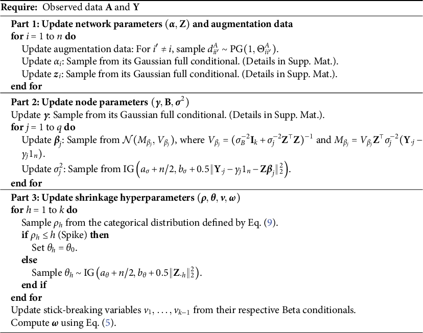
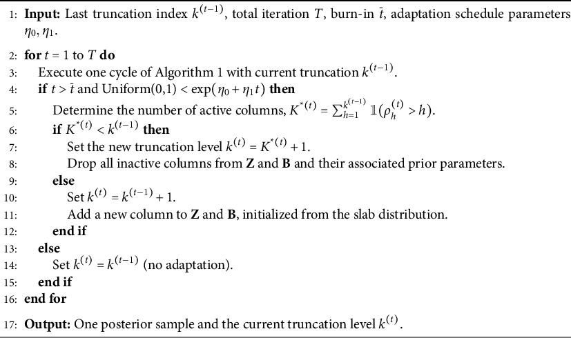
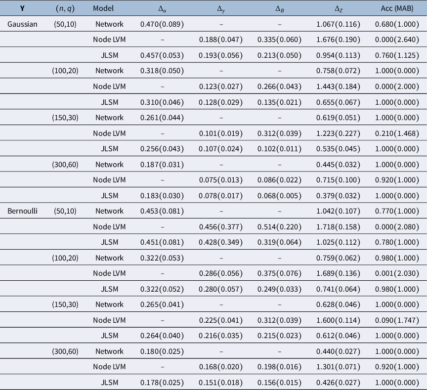

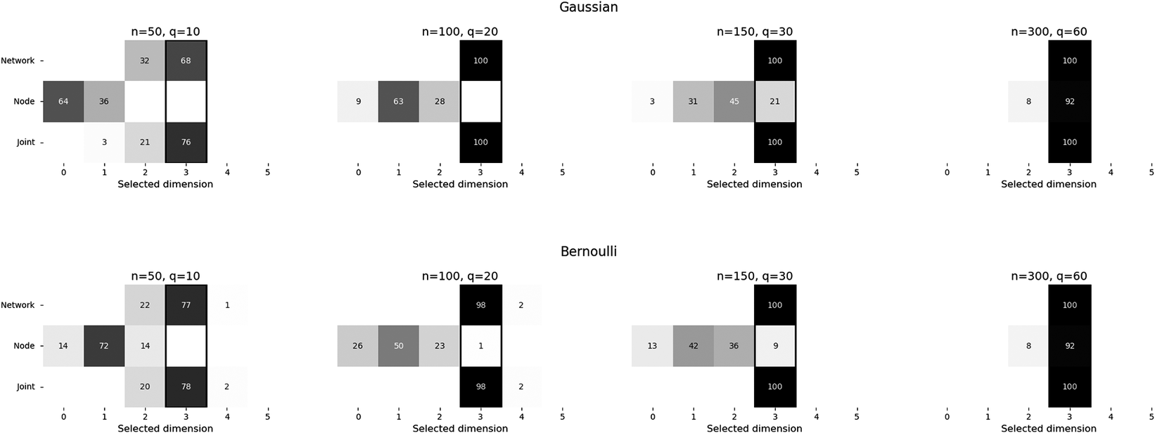

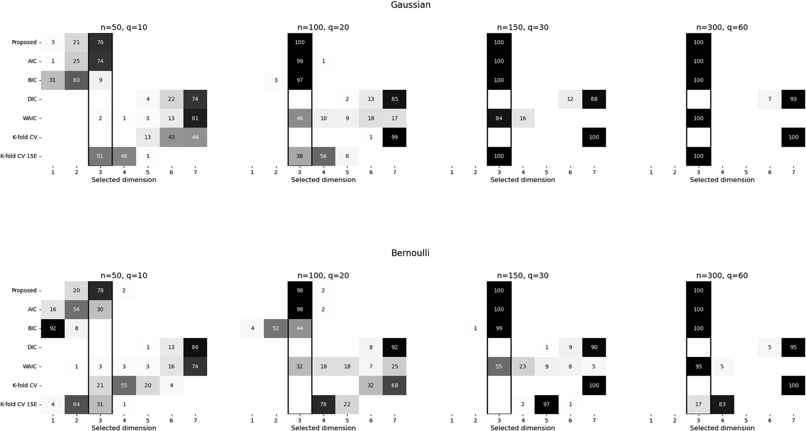


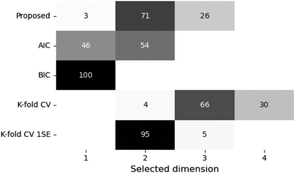
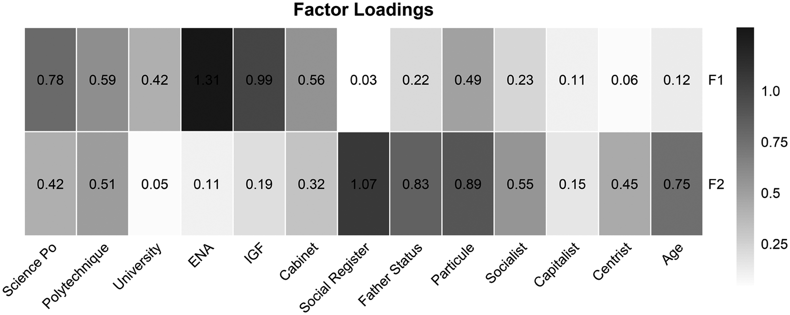


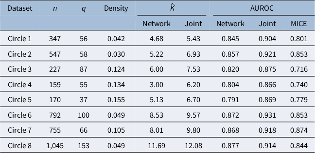
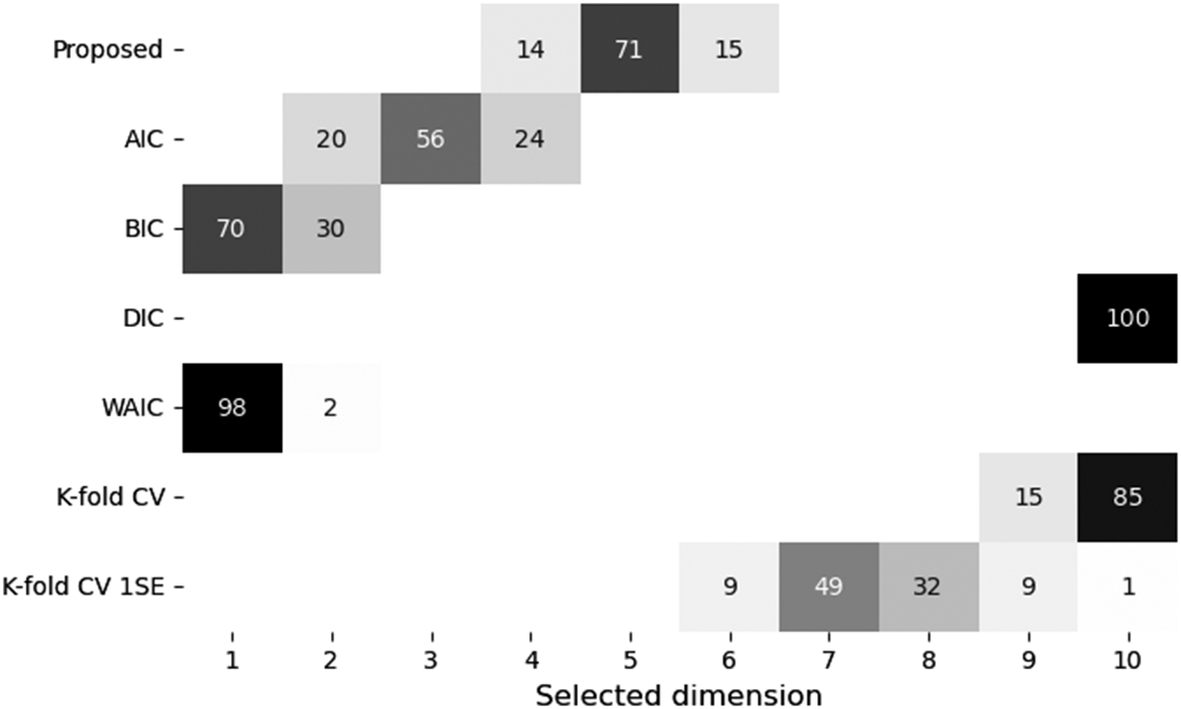



 Open access

