



1. Introduction
With the development of lean combustion aero-engines and land-based gas turbines, combustion instability has proven to be a persistent problem that can cause serious damage (Poinsot Reference Poinsot2017; Bailly et al. Reference Bailly, Durox, Juniper, Noiray, Poinsot, Schuller and Veynante2025). Combustion instability, also known as thermoacoustic instability, arises due to the interaction between flame heat release rate (HRR) fluctuations, oncoming flow perturbations upstream of the flame and acoustic oscillations in the combustion chamber (Candel Reference Candel2002). Its understanding and prediction require an understanding of how the flame HRR fluctuations respond to upstream velocity perturbations (Schuller, Durox & Candel Reference Schuller, Durox and Candel2003), often characterised by the ratio of the normalised HRR fluctuation to the normalised velocity perturbation. At low perturbation levels, the flame typically responds linearly to flow perturbations, and this relation is quantified using a flame transfer function (FTF) (Fleifil et al. Reference Fang, Yang, Hu, Wang, Li and Zheng1996). As the perturbation amplitudes increase, the flame response becomes nonlinear, and in the case of weak nonlinearity, is often characterised by a flame describing function (FDF) (Dowling Reference Cuquel, Durox and Schuller1997).
The FDF can be characterised through experiments (Noiray et al. Reference Noiray, Durox, Schuller and Candel2008; Durox et al. Reference Durox, Schuller, Noiray and Candel2009; Tian et al. Reference Tian, Nan, Yang and Li2024a
) and numerical simulations (Krediet et al. Reference Kedia, Altay and Ghoniem2013; Qiao & Lv Reference Qiao and Lv2023). A simpler alternative, which is able to quantitatively describe the FTF/FDF for laminar flames (Schuller et al. Reference Schuller, Durox and Candel2003; Orchini & Juniper Reference Orchini and Juniper2016a
; Tian et al. Reference Weng, Li, Zhong and Zhu2023; Qiao & Lv Reference Qiao and Lv2024; Tian et al. Reference Tian, Nan, Yang and Li2024b
) and weakly turbulent flames (Palies et al. Reference Palies, Durox, Schuller and Candel2011; Jiang et al. Reference Jiang and Peng2022), derives the flame model from the
 $G$
-equation proposed by Markstein (Reference Markstein1964) for tracking infinitely thin flame fronts. Based on the linearisation of the
 $G$
-equation for inclined flames, Schuller et al. (Reference Schuller, Durox and Candel2003) derived an analytical unified model which included the convective effects of flow modulation upstream of the flame to quantify the FTF of laminar premixed flames. The obtained analytical solution was in good agreement with the experimental results (Schuller et al. Reference Schuller, Ducruix, Durox and Candel2002). Lieuwen (Reference Lamraoui, Richecoeur, Schuller and Ducruix2005) developed a nonlinear framework for the
 $G$
-equation to analyse the nonlinear dynamics of a premixed flame in response to harmonic velocity perturbations and was able to predict the experimentally observed nonlinear behaviour of the flame (Bellows et al. Reference Bellows, Bobba, Forte, Seitzman and Lieuwen2007).
A more comprehensive characterisation of the nonlinear flame response is possible by considering perturbations at two or even more frequencies. As well as offering a more complete understanding of the flame nonlinearity, such studies are also directly relevant to experiments (Balachandran, Dowling & Mastorakos Reference Balachandran, Dowling and Mastorakos2008; Lamraoui et al. Reference Cuquel, Durox and Schuller2011; Albayrak et al. Reference Albayrak, Steinbacher, Komarek and Polifke2018; Fang et al. Reference Emmert, Bomberg and Polifke2021) and numerical simulations (Haeringer, Merk & Polifke Reference Gelb and Velde2019; Haeringer & Polifke Reference Haeringer, Merk and Polifke2019; Tathawadekar et al. Reference Tian, Liang, Zhang, Zhang, Yang and Li2021) exhibiting dual- or multiple-frequency oscillations.
Balachandran et al. (Reference Balachandran, Dowling and Mastorakos2008) conducted experiments investigating the nonlinear response of premixed flames at two different frequencies. With the introduction of subharmonics or higher harmonics, the formation and shedding of vortices change significantly. They elaborated on the possibility of suppressing instabilities by introducing additional excitation at carefully chosen frequencies to the flame. Based on the FDF framework, Boudy et al. (Reference Boudy, Durox, Schuller and Candel2011) further investigated nonlinear combustion instabilities in a multipoint injection combustor. Their results demonstrated that interactions between coexisting oscillation modes under dual-frequency forcing substantially alter the flame response, giving rise to nonlinear behaviours such as mode switching and hysteresis that cannot be captured by linear models. Lamraoui et al. (Reference Cuquel, Durox and Schuller2011) experimentally investigated combustion instability in a turbulent vortex burner with two non-harmonically related unstable modes at 180 and 280 Hz. The flame dynamics and corresponding combustion instabilities change significantly due to the presence of an additional disturbance. Similar modal interaction phenomena have also been reported in Rijke burner experiments, where the coupling between low-frequency flame pulsations and thermoacoustic modes gives rise to self-sustained amplitude modulation and beating (Weng et al. Reference Xu, Zheng, Wang, Feng, Tian, Li and Qi2016).
In this context, the analysis related to the nonlinear response under dual- or multi-frequency excitation can be broadly categorised into higher harmonics and non-resonant frequencies of the flame response. In the former case, Haeringer et al. (Reference Gelb and Velde2019) proposed an extended FDF based on the experimental phenomena of Albayrak et al. (Reference Albayrak, Steinbacher, Komarek and Polifke2018) as an efficient way to include higher harmonics of the flame response. More specifically, Han, Yang & Mao (Reference Haeringer and Polifke2016) numerically examined the nonlinear response of a lean premixed flame subjected to two strong perturbations at 160 and 320 Hz. The introduction of the higher-frequency forcing markedly altered HRR fluctuations, leading to a 70 % reduction in the flame response at the fundamental frequency compared with single-frequency excitation. In a practical combustion system (Lamraoui et al. Reference Cuquel, Durox and Schuller2011), however, perturbations frequently involve frequency pairs that are not harmonically related, leading to more complex nonlinear flame responses than those arising from correlated frequencies. As linear analysis shows a pattern with more than one positive growth rate, it is difficult to determine the presence and stability of steady-state oscillations.
Ćosić et al. (Reference Ćosić, Bobusch, Moeck and Paschereit2012) investigated open-loop forcing at non-resonant frequencies from the point of view of the nonlinear response of a flame to the superposition of two approximately sinusoidal input signals. They found that the reduction of the fundamental harmonic gain at unstable frequencies by additional forcing at non-resonant frequencies is a possible indicator of the success of open-loop control. Moeck & Paschereit (Reference Moeck and Paschereit2012) proposed conditions for the existence and stability of single- or multi-mode steady-state oscillations and applied this method to a thermoacoustic model with two linearly unstable modes. In the case of considering static nonlinearities, Gelb & Velde (Reference Fleifil, Annaswamy, Ghoneim and Ghoniem1968) obtained a large number of results in the study of two-frequency describing functions, most of whose properties are still applicable to dynamic nonlinearities.
Orchini & Juniper (Reference Orchini and Juniper2016b
) presented the computation of a non-static flame dual-input describing function based on the
 $G$
-equation model of a laminar conical flame. To perform harmonic balance analysis, they neglected the harmonic response at higher frequencies and assumed that the HRR response is dominated by components at the two input frequencies. It was able to predict the onset of the Neimark–Sacker bifurcation and determine the frequency of oscillations around the limit cycle. However, as noted by Orchini & Juniper (Reference Orchini and Juniper2016b
), this simplification becomes less appropriate when nonlinear coupling between multiple inputs generates additional low-frequency components, such as flame responses at
 $|\omega _1 \pm \omega _2|$
, where
 $\omega _1$
and
 $\omega _2$
denote the input angular frequencies. Along similar lines, Zheng et al. (Reference Zheng, Li, Wang, Xu, Wang, Xia and Qi2024) experimentally investigated the nonlinear flame response under dual-frequency excitation and explicitly examined the generation of interaction frequencies. Using a third-order asymptotic expansion of the
 $G$
-equation under the assumption of a fixed disturbance convection velocity, they demonstrated the emergence of a pronounced difference-frequency component (e.g.
 $|\omega _1 - \omega _2|$
), highlighting the second-order nonlinear interactions responsible for interaction-frequency generation.
Recently, the thermoacoustic response of hydrogen-enriched premixed flames subjected to non-harmonically related dual-mode forcing has been investigated using an FDF coupled with a low-order network model (Tian et al. Reference Tian, Nan, Yang and Li2024b ). The results demonstrated that dual-frequency coupling can substantially modify the nonlinear flame dynamics, leading to mode competition, suppression or amplification of the primary response and the emergence of difference-frequency oscillations. Building upon these findings, Tian, Yang & Li (Reference Tian, Yang, Morgans and Li2026) showed that such difference-frequency oscillations may become dominant through nonlinear modal interactions that are not captured by conventional single-input FDFs. To overcome this limitation, they introduced a dual-input FDF framework that enables frequency-domain modelling of cross-frequency coupling and difference-frequency generation, thereby improving predictive capability in multi-mode thermoacoustic systems.
These studies demonstrate that experimental, theoretical and numerical approaches involving dual- or multi-frequency perturbations provide deeper insights into flame nonlinearities and offer promising strategies for controlling combustion instabilities. However, despite the recognised influence of non-resonant frequency disturbances on the primary flame response, the underlying mechanisms governing the interaction between uncorrelated frequencies remain insufficiently understood. Specifically, in most of these studies, the flame module is treated as a ‘black box’ within the thermoacoustic network, thereby overlooking the underlying mechanisms responsible for the nonlinear flame response under dual- or multi-frequency perturbations. This limits physical understanding of the nonlinear flame response and further restricts its application in more practical cases.
As mentioned above, there is a deviation in the nonlinear flame response to a perturbation at frequency
 $St_1$
(
 $St$
is the Strouhal number, defined by the angular frequency multiplied by the spatial distance divided by the mean bulk velocity), when there is also a simultaneous excitation at a different frequency
 $St_2$
, compared with when
 $St_1$
is the only excitation frequency. In this study, the impact of the disturbance at
 $ St_2$
on the nonlinear flame response at
 $ St_1$
will be investigated. While Zheng et al. (Reference Zheng, Li, Wang, Xu, Wang, Xia and Qi2024) examined the generation of a flame response at different frequencies induced by excitation at
 $ St_2$
, the present study instead focuses on the suppression of the flame response at the primary frequency. This analysis will be conducted for general cases where the frequency, amplitude and phase of the perturbation at
 $ St_2$
are independent of those at
 $ St_1$
. In general, the nonlinear response of a V-flame to excitation is much more pronounced than that of a conical flame as the perturbation amplitude varies, as illustrated by the experiments of Durox et al. (Reference Durox, Schuller, Noiray and Candel2009). It is more appropriate to explore the above targets within the framework of V-flames with a more intense nonlinear response, so that it can be more clearly identified how the nonlinear response of the flame to excitation changes with the introduction of additional excitation at different frequencies.
In this paper, the spatial distribution of flame kinematics and the HRR response will be considered to quantify and account for the full nonlinearity induced by the dual-frequency excitation. The nonlinear results for the flame response are derived by considering a low-order asymptotic analysis (up to the third order in normalised excitation amplitude) applied to numerical computation of the flame based on the model framework of the
 $G$
-equation. Key empirical parameters are obtained from the experimental data and combined with results from a velocity-potential model to derive the dependence of the propagation speed of the disturbance on
 $St$
. These are described in § 2. The mechanisms by which the perturbation at
 $St_2$
affects the spatial kinematics of the flame at
 $St_1$
are discussed. These results are presented in § 3. The role of the perturbation at
 $St_2$
in the global flame response at
 $St_1$
is quantified, and the corresponding mechanisms are carefully discussed in § 4.
2. Formulation
This section presents analytical and numerical methods for determining the nonlinear acoustic response of laminar premixed V-flames to dual-frequency perturbations. As shown in figure 1, using the cylindrical coordinate system
 $x-r-\theta$
(
 $x$
,
 $r$
and
 $\theta$
correspond to the axial, radial and angular directions, respectively), an axisymmetric V-flame is anchored on the rim of the burner and subjected to the mean bulk velocity
 $\bar {u}$
and two velocity perturbations
 $u_1^\prime$
and
 $u_2^\prime$
with different frequencies and amplitudes. The instantaneous positions of the perturbed premixed flame can be captured by the
 $G$
-equation introduced by Markstein (Reference Markstein1964) to track the propagation of unsteady convected interfaces
 \begin{align} \frac {{\partial G}}{{\partial t}} + {\boldsymbol{u}} \boldsymbol{\cdot }\boldsymbol{\nabla }G = {S_L}\left | {\boldsymbol{\nabla }G} \right | , \end{align}
where
 $G$
is a scalar level-set function,
 $t$
is time,
 $\boldsymbol{u}$
is the velocity vector of a given flow field, i.e.
 $\boldsymbol{u}=(u,u_r,u_\theta )$
and
 $S_L$
is the laminar flame speed. The
 $G$
-(2.1) in this work assumes that: (i) an infinitely thin flame front (
 $G=0$
) separates the unburned reactant region (
 $G\lt 0$
) and burned gas region (
 $G\gt 0$
); (ii) the flame laminar displacement speed is constant, which assumes a spatially and temporally constant equivalence ratio and omits the flame curvature effect; (iii) the flow field upstream of the flame front can be predefined, and both heat diffusion and thermal expansion are neglected, implying weak density change across the flame front; and (iv) the flame height is a single-valued function of the radial coordinate.
Sketch of the perturbed V-flame subjected to dual-frequency disturbances. Here,
 $x$
,
 $r$
and
 $\theta$
denote the spatial coordinates;
 $\xi (r,\theta ,t)$
is the flame-front location;
 $u_1^\prime$
and
 $u_2^\prime$
are the perturbations at
 $St_1$
and
 $St_2$
, respectively;
 $\bar {u}$
is the mean bulk velocity;
 $\it \varOmega$
is the outer burner radius; and
 ${\it \varOmega }_b$
is the inner burner radius.

Figure 1. Long description
The diagram illustrates a perturbed V-flame subjected to dual-frequency disturbances. It features spatial coordinates labeled as x and r, with the flame-front location denoted by ξ(r, θ, t). The perturbations at two different frequencies are represented by u'1 and u'2. The mean bulk velocity is indicated by u with a bar, and the outer and inner burner radii are labeled as Ω and Ωb, respectively. The flame is depicted with red and blue regions, and the perturbations are shown with wavy arrows. The diagram includes directional arrows for the mean bulk velocity and perturbations, as well as a rotational arrow indicating the angular coordinate θ.
Equation (2.1) is rewritten as
 \begin{align} \frac {{\partial G}}{{\partial t}} + u\frac {{\partial G}}{{\partial x}} + {u_r}\frac {{\partial G}}{{\partial r}} + \frac {{{u_\theta }}}{r}\frac {{\partial G}}{{\partial \theta }} = {S_L}\sqrt {{{\left ( {\frac {{\partial G}}{{\partial x}}} \right )}^2} + {{\left ( {\frac {{\partial G}}{{\partial r}}} \right )}^2} + {{\left ( {\frac {1}{r}\frac {{\partial G}}{{\partial \theta }}} \right )}^2}} . \end{align}
According to assumption (iv),
 $G ({x,r,\theta ,t} )$
can be transformed into explicit form with respect to the instantaneous flame front
 $\xi ({r,\theta ,t} )$
. This means that, for a given radial position, only one axial position of the flame front is possible at a given instant. Although this is not entirely consistent with experimental observations, which show large sharp angles and different axial positions of the flame front for a given radius, it captures the main features of nonlinear flame response to excitations in both laminar and weakly turbulent cases (Hemchandra, Peters & Lieuwen Reference Han, Yang and Mao2011; Jiang et al. Reference Jiang and Peng2022)
 \begin{align} G\left ({x,r,\theta ,t} \right ) = x - \xi \left ( {r,\theta ,t} \right ) . \end{align}
Substituting (2.3) into (2.2), the flame front is
 $\theta$
-independent due to the angular symmetry of the mean flow and incoming flow perturbations (Lieuwen Reference Lamraoui, Richecoeur, Schuller and Ducruix2005; Preetham, Santosh & Lieuwen Reference Preetham, Santosh and Lieuwen2008). After further simplification, lower-order models based on the
 $G$
-equation have been proposed in the literature (Schuller et al. Reference Schuller, Durox and Candel2003; Preetham et al. Reference Preetham, Santosh and Lieuwen2008). Assuming that the incoming mean bulk velocity has only an axial component and lacks a corresponding radial component (
 $\bar {u}_r=0$
), the governing equation for the flame-front location
 $\xi$
is then recast as
 \begin{align} \frac {{\partial \xi }}{{\partial t}} - u + u^{\prime }_r\frac {{\partial \xi }}{{\partial r}}= - {S_L}\sqrt {1 + {{\left ( {\frac {{\partial \xi }}{{\partial r}}} \right )}^2}} , \end{align}
where
 $u^{\prime }_{r}$
is the radial velocity perturbation.
With the flame anchored on the burner rim, a boundary condition for (2.4) can be expressed as
 \begin{align} \xi \left ( {r = {\it \varOmega _b},t} \right ) = 0 , \end{align}
where
 $\it \varOmega _b$
is the radius of the centre body. In the remainder of this paper, all parameters are normalised, that is, velocities are normalised by the mean bulk velocity
 $\bar u$
, spatial coordinates are normalised by the burner radius
 $\it \varOmega$
and time by
 ${\it \varOmega }/\bar u$
.
2.1. Frequency-dependent model for incoming velocity perturbations
For the upstream velocity field of the flame, once the axial velocity perturbation
 $u^{\prime }$
is specified, the radial perturbation
 $u^{\prime }_r$
is not an independent quantity but is determined from the continuity equation under the incompressible and irrotational flow assumptions. This results in a radial velocity component that varies linearly with
 $r$
and depends on forcing frequency, as discussed in Cuquel, Durox & Schuller (Reference Cuquel, Durox and Schuller2011). Consequently, inclusion of the radial perturbation term in (2.4) leads to non-physical results for the V-flame response. Specifically, the intensity of the
 $u^{\prime }_{r}$
at the tip of the V-flame is excessively high and further amplifies the flame response within the context of the
 $G$
-equation, especially at high frequencies, which is physically unrealistic. Therefore, zero radial fluctuation is assumed (
 $u^{\prime }_{r}=0$
) in (2.4) despite the discontinuity in the prescribed velocity field. It should be noted that this treatment may represent a limitation of the present framework because the configuration considered in Cuquel et al. (Reference Cuquel, Durox and Schuller2011) differs from the present flame configuration, where heat release and finite flame extent may affect the radial convection dynamics. The issue related to neglecting
 $u^{\prime }_r$
is not encountered in the case of the conical flame that is axially perturbed because of its centred flame tip. The influence of the neglected radial perturbation term
 $u^{\prime }_r$
will be reconsidered using an alternative approach in the subsequent model construction.
Therefore, the velocity can be decomposed into a mean component and two perturbations of distinct frequencies and amplitudes originating from the thermoacoustic system
 \begin{align} u\left ( {S{t_1},S{t_2},x,t} \right )/\bar {u} = 1 + {\epsilon _1}{{C}_1}\left ( {S{t_1},x,t} \right ) + {\epsilon _2}{{C}_2}\left ( {S{t_2},x,t,\delta } \right ) . \end{align}
Herein,
 $C$
is the individual component of acoustic excitation and
 $\epsilon$
denotes the non-dimensional amplitude;
 $St=\omega {\it \varOmega }/\bar {u}$
is the normalised angular frequency;
 $\omega$
is the angular frequency. The subscripts ‘1’ and ‘2’ denote the perturbations at
 $St_1$
and
 $St_2$
, respectively, and
 $\delta$
denotes the initial phase difference between two perturbing components. The specific forms of the perturbation sources are given by
 \begin{align} \left \{ \begin{array}{l} {C_1}\left ( {S{t_1},x,t} \right ) = \cos \left [ {S{t_1}\left ( {K_1 x - t} \right )} \right ],\\[5pt] {C_2}\left ( {S{t_2},x,t,\delta } \right ) = \cos \left [ {S{t_2}\left ( {K_2 x - t} \right ) + \delta } \right ]. \end{array} \right . \end{align}
Here,
 $K_1$
and
 $K_2$
characterise the disturbance convection velocity
 $u_c$
and are expressed as
 $\bar u/u_c$
. It is frequently simplistically assumed that perturbations convect either with the mean volumetric velocity or with the sound speed, corresponding to
 $K=1$
or
 $K\to 0$
, respectively. Although this assumption is relatively straightforward, it typically fails to accurately reflect the actual convective behaviour observed in experiments or numerical simulations.
For instance, experimental studies (Birbaud, Durox & Candel Reference Birbaud, Durox and Candel2006; Karimi et al. Reference Jiang, Li, Yang and Liu2009; Yang et al. Reference Yang, Fang, Zhong, Xia, Jin, Li and Wang2011) and numerical simulations (Blanchard et al. Reference Blanchard, Schuller, Sipp and Schmid2015) have highlighted that the propagation of disturbances changes significantly as the modulation frequency upstream of the flame changes. Recent work (Steinbacher & Polifke Reference Tathawadekar, Doan, Silva and Thuerey2022) has emphasised that the need to calibrate
 $u_c$
arises from neglecting thermal diffusion and thermal expansion in the
 $G$
-equation model. The propagation of the disturbance along the flame sheet and the feedback to the velocity disturbances are responsible for
 $u_c$
. Therefore,
 $K$
in the
 $G$
-equation should be considered as an input parameter that requires calibration. However, in reality, propagation velocities cannot be an independent ‘input’ because they are determined by the closed-loop feedback of flame–flow interactions. This study proposes a simplified derivation (referred to as low-order modelling), which builds upon and extends the work of Birbaud et al. (Reference Birbaud, Durox and Candel2006). Its objective is to avoid the aforementioned conflicts while encapsulating the key characteristics of the relationship between
 $St$
and
 $K$
.
Within the velocity-potential framework, the radial velocity perturbation
 $u^{\prime }_{r}$
enters the formulation implicitly through its contribution to the
 $St$
–
 $K$
relation, thereby influencing the flame kinematics without appearing explicitly in the flame-front equation. With
 $z=1-r$
, a coordinate transformation is used to simplify the derivation process. Assuming the flow is incompressible and irrotational upstream of the flame, the velocity potential
 $\psi$
satisfies the Laplace equation and is written in cylindrical coordinates as
 \begin{align} \frac {{{\partial ^2}\psi }}{{\partial {x^2}}} + \frac {1}{z}\frac {{\partial \psi }}{{\partial z}} + \frac {{{\partial ^2}\psi }}{{\partial {z^2}}} = 0. \end{align}
Due to the presence of disturbances,
 $\psi$
is assumed to be in a wave-like form (i.e.
 $K_x$
, corresponding to axial perturbation propagation, is assumed to be unity)
 \begin{align} \psi = g\left ( z \right )\exp \left [ {\textrm {i}St\left ( {x - t} \right )} \right ]. \end{align}
Substituting (2.9) into (2.8), the ordinary differential equation for the radial velocity-potential distribution becomes
 \begin{align} \frac {{{{{d}}^2}g\left ( z \right )}}{{{\mathrm{d}}{z^2}}} + \frac {1}{z}\frac {{{\mathrm{d}}g\left ( z \right )}}{{{ \mathrm{d}}z}} - St^2 g\left ( z \right ) = 0. \end{align}
The general solution is
 \begin{align} g\left ( z \right ) = {A_1}{I_0}\left ( {Stz} \right ) + {A_2}{K_0}\left ( {Stz} \right ), \end{align}
where
 $I_0$
and
 $K_0$
are the zeroth-order modified Bessel functions.
The radial velocity component vanishes on the centreline
 $z=0$
, i.e.
 ${\left . {\partial \psi /\partial z} \right |_{z = 0}}=0$
, resulting in
 $A_2=0$
.
Following the approach of Birbaud et al. (Reference Birbaud, Durox and Candel2006), it is assumed that the flame front is nearly vertical, i.e. the flame half-angle is small. Under this assumption, flame wrinkles are considered to affect the radial velocity. One may write
 \begin{align} {\left . \frac {\partial \psi }{\partial z} \right |_{z =\eta (x)}} =B\cos \alpha \exp \left [ {\textrm {i}St\left ( {x - t} \right )} \right ], \end{align}
where
 $\eta (x)$
is the inverse function of
 $\xi (z)$
, denoting the flame front,
 $B$
denotes a pre-exponential coefficient and
 $\alpha$
is the half-angle of the flame tip.
Substituting (2.9) into (2.12), one obtains
 \begin{align} g\left ( z \right ) = B{I_0}\left ( {Stz} \right )/{I_1}\left ( {St{\eta (x)}} \right ), \end{align}
corresponding to the velocity-potential solution as follows:
 \begin{align} \psi \left ( {St,z,x} \right ) = \frac {{B{I_0}\left ( {Stz} \right )}}{{{I_1}\left [ {St\eta \left (x\right )} \right ]}}\exp \left [ {\textrm {i}St\left ( {x - t} \right )} \right ]. \end{align}
Thus, the relative velocity potential
 $\vartheta$
, defined as the ratio of the velocity potential on the reactant side to that on the flame front, is given by
 \begin{align} \vartheta \left ( {St,z,x} \right ) = \frac {{{I_0}\left ( {Stz} \right )}}{{{I_0}\left [ {St\eta \left ( x \right )} \right ]}}. \end{align}
It is shown in kinematic analyses and experiments that the acoustic wave can produce convective wrinkling on the flame front subjected to acoustic modulation, i.e.
 $K_\eta = 1$
. Therefore, the ratio of localised perturbation propagation velocities (
 $\kappa = \bar u/u_c (z,x )$
) at different spatial locations upstream of the flame can be derived using the parameter
 $\vartheta$
.
To further relate
 $\kappa$
to the relative velocity potential, an important empirical value of
 $\varLambda$
is used to relate the model results to the experimental data. If
 $\vartheta$
is smaller than the threshold
 $\varLambda$
, the perturbation speed is assumed to be the speed of sound, i.e.
 \begin{align} \kappa \left ( {St,z,x} \right ) = 0\,{\mathrm{when}}\, \vartheta \left ( {St,z,x} \right ) \lt \varLambda . \end{align}
Conversely, when
 $\vartheta$
exceeds
 $\varLambda$
, the perturbation is convected by the mean bulk velocity, i.e.
 \begin{align} \kappa \left ( {St,z,x} \right ) = 1 \, {\mathrm{when}} \,\vartheta \left ( {St,z,x} \right ) \ge \varLambda . \end{align}
Then the essential issue is to determine the threshold value
 $\varLambda$
from the experimental results. In the framework of conical flames, Birbaud et al. (Reference Birbaud, Durox and Candel2006) assumed a threshold of
 $\varLambda = 0.1$
, and the corresponding modelling results were shown to be in good agreement with experimental velocity perturbations measured upstream of the flame by particle image velocimetry (PIV). Recently, Yang et al. (Reference Yang, Fang, Zhong, Xia, Jin, Li and Wang2011) conducted similar experiments and found that
 $\varLambda =0.2$
represented the experimental results better. Figure 2 presents a comparison of the modelling results for two different
 $\varLambda$
cases with the experiments, where the modelling of the conical flame is also derived from (2.8)
 $\sim$
(2.17), but here
 $z$
is
 $r$
instead of
 $1-r$
. For details on obtaining experimental data from Birbaud et al. (Reference Birbaud, Durox and Candel2006), see Appendix A. The physical meaning of
 $\varLambda$
can be interpreted as follows:
 $\varLambda$
strongly influences the propagation behaviour of these perturbations by altering
 $\kappa$
through (2.16) and (2.17). As
 $\varLambda$
increases,
 $u_c$
approaches the speed of sound more readily. Based on comparison with the experimental data,
 $\varLambda = 0.2$
provides better agreement and is therefore adopted for the remainder of this study.
It should be noted that the existing studies (Birbaud et al. Reference Birbaud, Durox and Candel2006; Yang et al. Reference Yang, Fang, Zhong, Xia, Jin, Li and Wang2011) pertain exclusively to conical flames, and no comparable results are currently available for the determination of
 $\varLambda$
in V-flames. Therefore, in the case of V-flames,
 $\varLambda$
must be inferred from experimental data for conical flames in order to more realistically reveal how the upstream value of
 $\kappa$
varies with spatial position. The V-flame considered here is a simplified version of an inverted conical laminar flame, with the effect of vorticity on flame kinematics being neglected. This greatly reduces the differences between V-flames and conical flames, thereby justifying the application of the
 $\varLambda$
value derived from conical flames to V-flames. Indeed, these simplifications appear to be reasonable, as will be demonstrated through subsequent experiments and model comparisons (see § 4).
Comparison between the model predictions and experimental results for the ratio of the localised perturbation propagation velocity
 $\kappa$
along the centreline of a conical flame. From left to right:
 $f=250$
,
 $f=130$
and
 $f=50$
Hz. Experimental data reproduced from Birbaud et al. (Reference Birbaud, Durox and Candel2006).

Figure 2. Long description
The image contains three line graphs side by side, each comparing model predictions and experimental results for the ratio of localized perturbation propagation velocity along the centerline of a conical flame. The x-axis represents normalized flame height, ranging from 0 to 1. The y-axis represents the variable kappa, ranging from -0.5 to 1.5. Each graph includes experimental data points marked by blue circles. Two model predictions are shown: one with a solid yellow line for lambda equals 0.2 and another with a dotted red line for lambda equals 0.1. The graphs illustrate how the model predictions align with the experimental data across different conditions. All values are approximated.
Dependence of
 $K$
on
 $St$
for the V-flame. Here,
 $\varLambda =0.2$
,
 ${\it \varOmega _b}=0$
.

Figure 3. Long description
A line graph showing the dependence of K on St for the V-flame. The x-axis represents St values ranging from 0 to 40, while the y-axis represents K values ranging from 0 to 1. The graph depicts a downward trend, indicating that as St increases, K decreases. All values are approximated.
A global parameter
 $K$
, which characterises the overall properties of the reactant side, is defined as
 \begin{align} K\left ( {St} \right ) = \int _{\theta = 0}^{2\pi } {{\mathrm{d}}\theta \int _{x} {\int _{z } {\kappa \left ( {St,z,x} \right )z{\mathrm{d}}} x{\mathrm{d}}z} } \Bigg /\int _{\theta = 0}^{2\pi } {{\mathrm{d}}\theta \int _{x} {\int _{z} z {\mathrm{d}}x{\mathrm{d}}z} }. \end{align}
The relation between
 $St$
and
 $K$
is illustrated in figure 3. At low frequencies, inflow disturbances propagate with the mean bulk velocity. As the modulation frequency increases, the disturbance propagation speed also increases. When the forcing frequency becomes sufficiently high,
 $u_c$
approaches the speed of sound. At intermediate frequencies, perturbation propagation exhibits mixed characteristics;
 $u_c$
varies with spatial position and is no longer uniform. The corresponding spatially averaged value,
 $\bar {u_c}$
, lies between
 $\bar u$
and
 $c$
. These three distinct types of frequency-dependent behaviour are qualitatively consistent with experimental observations (Birbaud et al. Reference Birbaud, Durox and Candel2006) and numerical simulations (Blanchard et al. Reference Blanchard, Schuller, Sipp and Schmid2015). It is important to note that this method cannot capture cases where
 $u_c\lt \bar {u}$
(
 $K\gt 1$
), as observed in certain spatial regions at specific frequencies in different cases (Birbaud et al. Reference Birbaud, Durox and Candel2006; Karimi et al. Reference Jiang, Li, Yang and Liu2009; Blanchard et al. Reference Blanchard, Schuller, Sipp and Schmid2015). However, most analytical studies on laminar premixed flames typically assume
 $K=0$
or
 $K=1$
, ignoring its dependence on modulation frequency (Zheng et al. Reference Zheng, Li, Wang, Xu, Wang, Xia and Qi2024). The present approach improves upon previous models by quantitatively linking
 $K$
to the influence of
 $St$
within the range from 0 to 1.
2.2. Low-order asymptotic analysis of the flame front
An asymptotic analysis of the governing equation is performed to reveal the underlying mechanisms of the nonlinear interaction between the two perturbations. Asymptotic analysis is extended up to third order in the excitation amplitudes
 $\epsilon _1$
and
 $\epsilon _2$
, as follows:
 \begin{align} \begin{split} \xi ({r,t})& = \underbrace {{\xi _0}(r)}_{{\mathrm{Steady \, term}}} + \underbrace {{\epsilon _1} {\xi _1}({r,t}) + {\epsilon _2} {\xi _2}({r,t})}_{{\mathrm{Linear\, terms}}}\\ & + \underbrace {{\epsilon _1}^2 {\xi _{1,1}}({r,t}) + {\epsilon _2}^2 {\xi _{2,2}}({r,t}) + {\epsilon _1}^3 {\xi _{1,1,1}}({r,t}) +{\epsilon _2}^3 {\xi _{2,2,2}}({r,t})}_{{\mathrm{Self-nonlinear\,terms}}}\\ &+ \underbrace {{\epsilon _1} {\epsilon _2} {\xi _{1,2}}({r,t}) + {\epsilon _1}^2 {\epsilon _2} {\xi _{1,1,2}}({r,t}) + {\epsilon _1}{\epsilon _2}^2 {\xi _{1,2,2}}({r,t})}_{{\mathrm{Mutual-nonlinear\,terms}}}\\ & + {O}\left [ {{{\big ( {{\epsilon _1},{\epsilon _2}} \big )}^4}} \right ] ,\end{split} \end{align}
where the subscript ‘0’ denotes the steady flame configuration. The subscripts ‘1’ and ‘2’ identify response components associated with excitations at frequencies
 $St_1$
and
 $St_2$
, respectively. For the flame front
 $\xi$
, the number of subscript indices indicates the order of the flame response in the perturbation expansion. A single index (e.g.
 $\xi _1$
or
 $\xi _2$
) represents a first-order flame response, two indices denote second-order contributions, and three indices correspond to third-order terms. The specific combination of indices identifies the frequency origin of the nonlinear flame response. For instance,
 $\xi _{1,1}$
represents a second-order self-nonlinear flame response arising from excitation at
 $St_1$
, whereas
 $\xi _{1,2}$
denotes a second-order mutual-nonlinear flame response resulting from the interaction between response components associated with excitations at
 $St_1$
and
 $St_2$
. Similarly,
 $\xi _{2,2,2}$
corresponds to a third-order self-nonlinear flame response associated exclusively with excitation at
 $St_2$
, while
 $\xi _{1,2,2}$
represents a third-order term resulting from the interaction between a first-order response to excitation at
 $St_1$
and a second-order response to excitation at
 $St_2$
. Each term is proportional to the corresponding product of perturbation amplitudes (e.g.
 $\epsilon _1^2$
,
 $\epsilon _1\epsilon _2$
or
 $\epsilon _1\epsilon _2^2$
), consistent with the associated subscript structure.
These ten terms can therefore be grouped into three categories: linear, self-nonlinear and mutual-nonlinear contributions. The linear and self-nonlinear terms correspond to responses induced by individual excitations at
 $St_1$
or
 $St_2$
, whereas the mutual-nonlinear terms arise from the coupled action of both excitations.
The steady-term solution for the V-flame can be easily obtained as follows:
 \begin{align} {\xi _{0}}(r) = r \cot \alpha . \end{align}
By substituting (2.19) into the nonlinear source term on the right-hand side of (2.4) and applying a Taylor expansion up to third order, the nonlinear term can be expressed as
 \begin{align} \sqrt {1 + {{\left ( {\frac {{\partial \xi }}{{\partial r}}} \right )}^2}} \approx {\iota _0}{\mathrm{ + }}{\iota _1}\left ( {\frac {{\partial \xi }}{{\partial r}} - \frac {{\partial {\xi _0}}}{{\partial r}}} \right ) + \frac {1}{2}{\iota _2}{\left ( {\frac {{\partial \xi }}{{\partial r}} - \frac {{\partial {\xi _0}}}{{\partial r}}} \right )^2} , \end{align}
where
 \begin{align} \begin{split} &{\iota _0} = {\left [ {1 + {{\left ( {\frac {{\partial {\xi _0}}}{{\partial r}}} \right )}^2}} \right ]^{1/2}};\\ &{\iota _1} = \frac {{\partial {\xi _0}}}{{\partial r}}{\left [ {1 + {{\left ( {\frac {{\partial {\xi _0}}}{{\partial r}}} \right )}^2}} \right ]^{ - 1/2}};\\ &{\iota _2} = {\left [ {1 + {{\left ( {\frac {{\partial {\xi _0}}}{{\partial r}}} \right )}^2}} \right ]^{ - 1/2}} - {\left ( {\frac {{\partial {\xi _0}}}{{\partial r}}} \right )^2}{\left [ {1 + {{\left ( {\frac {{\partial {\xi _0}}}{{\partial r}}} \right )}^2}} \right ]^{ - 3/2}}. \end{split} \end{align}
The nonlinear source term has a clear physical interpretation, representing the propagation of the flame along its normal direction.
Following the standard procedure of asymptotic analysis, the detailed solution of each term in (2.19) can be obtained. The specific forms of these terms are provided in Appendix B. Focusing on the main issue addressed in this work, the terms were analysed concisely, three of which ((B12), (B16) and (B20)) were found to be directly related to the flame kinematics under the perturbation at
 $St_1$
. The specific expression is given by
 \begin{align} \begin{split} {\xi _{S{t_1}}}({r,t}) & = \underbrace {{\epsilon _1}{\xi _1}({r,t})}_{{\mathrm{Linear\,solution}}} + \underbrace {{\epsilon _1}^3{\xi _{{{I}},{\mathrm{1}},{\mathrm{1}},{\mathrm{1}}}}({r,t})}_{{\mathrm{Self\hbox{-}nonlinear\,solution}}} + \underbrace {{\epsilon _1}{\epsilon _2}^2{\xi _{{{I}},{\mathrm{1}},{\mathrm{2}},{\mathrm{2}}}}({r,t})}_{{\mathrm{Mutual\hbox{-}nonlinear\,solution}}}\\ &={\epsilon _1}{{\mu _1}(r)} \cos \left [ {S{t_1}t + {\chi _1}(r)} \right ]+{\epsilon _1}^3{{\mu _{{{I}},1,1,1}}(r)} \cos \left [ {S{t_1}t + {\chi _{{{I}},1,1,1}}(r)} \right ]+\\ &\quad {\epsilon _1}{\epsilon _2}^2{{\mu _{{{I}},{\mathrm{1}},{\mathrm{2}},{\mathrm{2}}}}(r)} \cos \left [ {S{t_1}t + {\chi _{{{I}},{\mathrm{1}},{\mathrm{2}},{\mathrm{2}}}}(r)} \right ]\\ &={{\mu _{St_1}}(r)} \cos \left [ {S{t_1}t + {\chi _{St_1}}(r)} \right ] ,\end{split} \end{align}
where the subscript ‘
 $St_1$
’ denotes the solution at
 $St_1$
,
 $\mu (r )$
and
 $\chi (r )$
denote the amplitude and phase of the flame spatial response.
These three components have clear physical interpretations: the first term represents the linear response of the flame kinematics to excitation at
 $St_1$
, while the remaining two terms arise from the nonlinearity of flame kinematic restoration. The derivation of the two third-order terms in (2.23) can be determined based on low-order asymptotic analysis. The former (called the self-nonlinear term,
 $\xi _{{I},1,1,1}$
) is induced by perturbation at
 $St_1$
, and the second term (called the mutual-nonlinear term,
 $\xi _{{I},1,2,2}$
) arises from simultaneous excitations at both
 $St_1$
and
 $St_2$
. The term
 $\xi _{{I},1,2,2}$
is significant, as it directly modifies the flame response behaviour at
 $St_1$
under perturbation at
 $St_2$
. In other words,
 $\xi _{{I},1,2,2}$
represents the variation of flame kinematics at
 $St_1$
when an excitation at frequency
 $St_2$
is applied. This demonstrates that asymptotic analysis provides an efficient approach to assess the influence of linear, self-nonlinear and mutual-nonlinear responses arising from perturbations at
 $St_2$
and
 $St_1$
on flame kinematics at
 $St_1$
, ultimately enhancing the understanding of their role in flame-front tracking.
3. Flame kinematics
In this section, the spatial kinematics of V-flames at
 $St_1$
under two-frequency excitations are analysed asymptotically. Numerical methods are also employed by embedding the relation between
 $K$
and
 $St$
to directly solve for the flame front
 $\xi$
, and the corresponding results are presented to verify the analytical findings. Spatial discretisation is performed using the seventh-order weighted essentially non-oscillatory scheme (Jiang & Peng Reference Jiang and Peng2000). Because nodes are defined only within the computational domain, the spatial derivatives at the boundary nodes are discretised using the fifth-order accurate upwind-differencing scheme. For time integration, a five-stage, fourth-order strong stability-preserving Runge–Kutta method (Shu Reference Silva2009) is used. The local Lax–Friedrichs scheme (Jiang & Peng Reference Jiang and Peng2000) is applied to enhance stability. The spatial grid spacing is set to
 $2\pi St/ (200K )$
, and the temporal step size is determined according to the Courant–Friedrichs–Lewy (CFL) condition with
 $\textrm {CFL} =0.2$
.
It is assumed that the response includes all possible frequency interactions between
 $St_1$
and
 $St_2$
, while the sub-harmonics of the input frequencies are neglected. The double Fourier series expansion (Orchini & Juniper Reference Orchini and Juniper2016b
) is employed to represent the flame front, which can be written as
 \begin{align} \xi ({r,t}) = \sum \limits _m {\sum \limits _n { {{\mu ^N _{mSt_1+nSt_2}}(r)} } } \cos \left [ {\left ( {mS{t_1} + nS{t_2}} \right )t{ + }{\chi ^N _{mSt_1+nSt_2}}(r)} \right ]+\xi _0 \left ( {r} \right ) , \end{align}
where
 $m,n\in \mathbb{Z}$
, and the superscript ‘
 $N$
’ denotes numerically obtained results. As mentioned above, this study primarily focuses on the flame kinematics at
 $St_1$
; hence, only the numerical results corresponding to
 $St_1$
are extracted from (3.1).
Comparison between asymptotic and numerical predictions of the flame-front response at
 $St_1$
for the V-flame. Solid lines and markers denote the asymptotic and numerical results, respectively. Here,
 $\epsilon _1=0.2$
,
 $\epsilon _2=0.1$
,
 $\delta =\pi /4$
,
 $R=1.6$
,
 $R=St_2/St_1$
,
 $\cot \alpha =3$
and
 ${\it \varOmega _b}=0$
. The superscript ‘
 $N$
’ denotes numerical results.

Figure 4. Long description
A line graph comparing asymptotic and numerical predictions of the flame-front response for the V-flame with different St1 values. The x-axis represents the variable r ranging from 0 to 1, and the y-axis represents the ratio of μSt1/ε1 or μNSt1/ε1 ranging from 0 to 4. The graph includes three sets of data: St1 equals 0.1, St1 equals 5, and St1 equals 10. Each set is represented by solid lines for asymptotic results and markers for numerical results. The data for St1 equals 0.1 shows a linear increase, while the data for St1 equals 5 and St1 equals 10 show nonlinear responses. The markers for numerical results closely follow the solid lines for asymptotic results, indicating a good agreement between the two methods. All values are approximated.
Figure 4 compares the relative magnitudes of the numerical and asymptotic solutions for the flame-front response at
 $St_1$
under dual-frequency excitation. The spatial response amplitudes of the flame at
 $St_1$
obtained by asymptotic analysis agree well with those determined numerically across different perturbation cases. This demonstrates that asymptotic analysis is reliable for capturing the flame kinematics at
 $St_1$
under dual-frequency excitation (through (2.23)) and for analysing their formation path, i.e. the perturbation at
 $St_2$
modifies the flame spatial response at
 $St_1$
solely through the
 $\xi _{{I},1,2,2}$
term. In contrast, while the full numerical approach can produce reliable ensemble results at
 $St_1$
, it cannot classify and individually analyse these results based on their physical significance.
Relative flame-front response of the V-flame at
 $St_1$
. (a) Effect of excitation amplitude for
 $\delta =0$
. From left to right:
 $St_1=0.1$
and
 $R=0.3$
;
 $St_1=4.7$
and
 $R=0.9$
;
 $St_1=10$
and
 $R=0.6$
. (b) Effect of the initial phase difference between the two excitations for
 $\epsilon _1=\epsilon _2=0.1$
,
 $St_1=5$
and
 $R=1.2$
. The superscript ‘
 $N$
’ denotes numerical results. Here,
 $\cot \alpha =3$
,
 $R=St_2/St_1$
and
 ${\it \varOmega _b}=0$
.

Figure 5. Long description
The image contains four graphs. The first set of three line graphs on the top row shows the effect of excitation amplitude on the flame-front response of the V-flame. Each graph represents different combinations of excitation amplitudes. The x-axis represents the variable r, and the y-axis represents the normalized flame-front response. The second graph on the bottom row is a scatter plot showing the effect of the initial phase difference between the two excitations on the flame-front response. The x-axis represents the variable r, and the y-axis represents the normalized flame-front response. Different symbols represent different phase differences. All values are approximated.
When the forcing frequency is low or the flame position is located near the flame holder, the flame exhibits a purely linear response, and its characteristics are only marginally influenced by the perturbation frequency (see figure 4) and amplitude (see figure 5
a). A previous study (Shanbhogue et al. Reference Shanbhogue, Shin, Hemchandra, Plaks and Lieuwen2009) has reported similar results when the modulation frequency is low or the spatial position is close to the flame holder. The characteristics of the flame response are all governed by a spatial interference wavelength defined as
 $1/ [2\pi St (1-K ) ]$
. The reduced length scale may be either larger or smaller than the interference wavelength. In the former case, the spatial response amplitude of the flame exhibits multiple peaks, as shown in the case of
 $St_1=10$
in figure 5(a). With decreasing
 $St_1$
, the interference wavelength increases, causing the multiple peaks to disappear and giving rise to a single peak or no peak, as observed for
 $St_1=4.7$
and
 $St_1=0.1$
, respectively, in figure 5(a). These characteristics were also observed in certain experiments (Shanbhogue et al. Reference Shanbhogue, Shin, Hemchandra, Plaks and Lieuwen2009). As the amplitude of the dual-frequency excitation varies, the perturbation at
 $St_2$
exerts a stronger suppressive effect on the flame kinematic response at
 $St_1$
than the excitation at
 $St_1$
. In addition, the degree of suppression of the spatial response induced by the perturbation varies non-monotonically with excitation frequency (first increasing and then decreasing), indicating that the suppression is most pronounced at a critical frequency.
Flame-front response at
 $St_1$
for the V-flame. (a) Magnitude and phase of the linear, self-nonlinear and mutual-nonlinear contributions in (2.23). (b) Magnitude and phase of the resulting combined response at
 $St_1$
. Here,
 $St_1=8$
,
 $St_2=5$
,
 $\epsilon _1=\epsilon _2=0.2$
,
 $\cot \alpha =3$
and
 ${\it \varOmega _b}=0$
.

Figure 6. Long description
The image contains two line graphs side by side, each with multiple data series represented by different line styles and colors. The left graph (a) shows the magnitude and phase of the linear, self-nonlinear, and mutual-nonlinear contributions. The x-axis is labeled 'r' ranging from 0 to 1, and the y-axis is split into two parts: the top part labeled '|μx|' ranging from 0 to 2, and the bottom part labeled 'χx/π (rad)' ranging from -10 to 2. The data series are represented by a solid blue line for 'x = 1', a dashed red line for 'x = I, 1, 1, 1', and a dotted green line for 'x = I, 1, 2, 2'. The right graph (b) shows the magnitude and phase of the resulting combined response at a specific condition. The x-axis is labeled 'r' ranging from 0 to 1, and the y-axis is split into two parts: the top part labeled '|ξx,Sl|/ε1' ranging from 0 to 0.4, and the bottom part labeled '<ξx,Sl>/π (rad)' ranging from -4 to 0. The data series are represented by a solid blue line for 'x = PL', a dashed red line for 'x = PN', and a dotted green line for 'x = FN'. The graphs illustrate the flame-front response at a specific frequency for a V-flame, showing how different contributions and their combinations affect the response.
The underlying mechanisms of this phenomenon are analysed below. Figure 6(a) shows the magnitude and phase of each term in (2.23). At certain excitation frequencies, the magnitude of the self-nonlinear solution is smaller than that of the mutual-nonlinear solution (this relation depends on the modulation frequency). Their phases are identical (
 $\chi _{{I,1,1,1}}=\chi _{ {I,1,2,2}}$
), which are insensitive to the modulation frequency, since they both originate from the third-order partial differential equations (PDEs). More interestingly,
 $\xi _{1}$
,
 $\xi _{{I},1,1,1}$
and
 $\xi _{{I},1,2,2}$
are not affected by the initial phase difference
 $\delta$
between the two excitations; thus,
 $\xi _{S{t_1}}$
is also insensitive to
 $\delta$
(see figure 5
b). The terms
 $\xi _{1}$
and
 $\xi _{1,1,1}$
can be readily interpreted, as they are influenced solely by the excitation at
 $St_1$
. The latter induces
 $\xi _{{I},1,1,1}$
, which is naturally insensitive to
 $\delta$
. Here,
 $\xi _{1,2,2}$
, dominated by excitations at both
 $St_1$
and
 $St_2$
, produces
 $\xi _{{I},1,2,2}$
, which is likewise unaffected by
 $\delta$
. This characteristic has been confirmed by a related experimental study (Zheng et al. Reference Zheng, Li, Wang, Xu, Wang, Xia and Qi2022), supporting the validity of the present modelling results. Furthermore, these results can also be interpreted from another perspective: when
 $St_1$
and
 $St_2$
are incommensurate, the initial phase difference disappears after a few cycles and has no effect on the fundamental frequency response. Owing to the above characteristics, the following results are based on
 $\delta =0$
. Figure 6(b) shows that due to the introduction of nonlinear solutions (both the self-nonlinear and mutual-nonlinear terms, where
 $\xi _{PL, St_1}=\epsilon _1\xi _{1}$
,
 $\xi _{PN, St_1} = \epsilon _1\xi _{1} + {\epsilon _1}^3\xi _{{I},1,1,1}$
and
 $\xi _{FN, St_1} = {\xi _{S{t_1}}}$
), the magnitude and phase of the flame spatial response at
 $St_1$
are corrected based on the linear result. Among these, as the downstream distance increases, the amplitude of flame wrinkles decreases, and the phase-step phenomenon observed in the linear results is mitigated.
Relative difference between the mutual-nonlinear and self-nonlinear amplitudes for the V-flame: (a)
 $St_1=1$
; (b)
 $St_1=5$
; (c)
 $St_1=9$
. Here,
 $H_{St_1}(r)=\mu _{{I},1,2,2}(r)-\mu _{{I},1,1,1}(r)$
.
 $R=St_2/St_1$
,
 $\cot \alpha =3$
and
 ${\it \varOmega _b}=0$
.

Figure 7. Long description
A heat map displays the relative difference between mutual-nonlinear and self-nonlinear amplitudes for the V-flame. The heat map consists of three subplots labeled (a), (b), and (c). Each subplot has a color scale indicating the magnitude of the relative difference. The x-axis is labeled 'r' ranging from 0 to 1, and the y-axis is labeled 'R' ranging from 0 to 3. In subplot (a), the color scale ranges from 0 to 1.8, showing a gradient from light to dark blue. Subplot (b) has a color scale from 0 to 7, with a noticeable concentration of higher values around R equals 1, marked by a red line indicating St2 approximately equals 3.5. Subplot (c) features a color scale from 0 to 10.5, also with a concentration of higher values around R equals 1, marked by a red line indicating St2 approximately equals 3.5.
To compare directly the nonlinear effects of excitations at
 $St_1$
and
 $St_2$
on the spatial response of the flame at
 $St_1$
(which demonstrates the ability to correct the linear results), the relative value
 $H_{St_1} (r )$
of the mutual-nonlinear and self-nonlinear amplitudes is directly defined as
 $\mu _{{I},1,2,2} (r )-\mu _{{I},1,1,1} (r )$
, since their corresponding phases are always identical. As shown in figure 7, it is evident that the amplitude of the mutual-nonlinear term is larger than that of the self-nonlinear term, particularly near the flame tip, except within a narrow range of low forcing frequencies. As
 $St_2$
increases,
 $\mu _{{I},1,2,2} (r )$
exhibits a steady peak, increasing monotonically before decreasing. This peak represents the strongest effect of perturbation at frequency
 $St_2$
in suppressing the amplitude of flame wrinkles at
 $St_1$
. It is noteworthy that, regardless of
 $St_1$
, the steady peak of the mutual-nonlinear solution always exists and corresponds to the case of
 $St_2\approx 3.5$
, which is determined by the relation between
 $St$
and
 $K$
. The nonlinear solution usually varies monotonically with the modulation frequency or
 $u_c$
(
 $u_c\in [\bar u,c ]$
, where
 $c$
is the speed of sound) (Jiang et al. Reference Jiang and Peng2022). The effect of flame kinematic restoration makes smaller length-scale wrinkles (associated with smaller
 $u_c$
and larger
 $St$
) more prone to destruction, thereby enhancing the flame kinematic response associated with dissipation. However,
 $St$
and
 $u_c$
are negatively correlated (see figure 3), resulting in a stable peak of the nonlinear response.
4. Global nonlinear flame response
The HRR of a premixed flame can be determined by quantifying the perturbation area obtained through flame-front tracking (Schuller, Poinsot & Candel Reference Schuller, Poinsot and Candel2020). However, the presence of excitations alters the time-averaged ensemble kinematics of the flame (Acharya & Lieuwen Reference Acharya and Lieuwen2021), which in turn affects the effective displacement speed and HRR of the flame. This mechanism can be further elucidated through asymptotic analysis. Specifically, the terms
 $\xi _{1,1}$
and
 $\xi _{2,2}$
in (2.19) (see (B14) and (B15) for their explicit expressions) demonstrate that acoustic forcing generates a zero-frequency component, which modifies the time-averaged flame shape relative to the steady unforced state. The corresponding zero-frequency response will be examined in detail later.
This phenomenon, not previously documented in the literature, suggests that excitation can impact the global response of the flame through an alternative pathway. In particular, the flame displacement speed
 $S_{\textit{eff, disp}}$
employed in HRR calculations differs from that of a steady flame.
Building on the above analysis and (2.4), the flame displacement speed accounting for the time-averaged flame dynamics is given by
 \begin{align} {S_{\textit{eff,disp}}}(r) = \left \langle - \frac {{\partial \xi /\partial t - u }}{{{{\left [ {1 + {{\left ( {\partial \xi /\partial r} \right )}^2}} \right ]}^{1/2}}}}\right \rangle , \end{align}
where ‘
 $\left \langle {} \right \rangle$
’ denotes the time-averaged properties. A similar method has been employed in previous studies, e.g. Palies et al. (Reference Palies, Durox, Schuller and Candel2011). The quantity
 $\xi$
can be obtained either through the numerical approach or by asymptotic analysis, as given in (2.19). Notably, to ensure the accuracy of the results, the numerical approach is generally preferred. This preference arises because only
 $\xi _{St_1}$
obtained from asymptotic analysis has been validated against numerical solutions, whereas the general form of
 $\xi$
has not. Importantly, (4.1) is not used to determine the flame position itself, but rather to evaluate the effective flame displacement speed entering the HRR calculation.
Effective flame displacement speed
 ${S_{\textit{eff},\textit{disp}}}(r)$
for the V-flame: (a)
 $R=0$
(single-frequency forcing); (b)
 $R=2.2$
; (c)
 $R=3.6$
. Here,
 $R=St_2/St_1$
,
 $\epsilon _1=\epsilon _2=0.2$
,
 $\cot \alpha =3$
and
 ${\it \varOmega _b}=0$
.

Figure 8. Long description
The image contains three heat maps labeled (a), (b), and (c), each representing the effective flame displacement speed for the V-flame under different conditions. The heat maps use a color scale ranging from 0.93 to 1.01 to indicate the values of the effective flame displacement speed normalized by the laminar burning velocity. The x-axis represents the variable r, ranging from 0 to 1, while the y-axis represents the Strouhal number St1, ranging from 0 to 10. Each heat map shows a gradient of colors, with darker shades indicating lower values and lighter shades indicating higher values. The patterns in the heat maps suggest variations in the effective flame displacement speed as the modulation frequency upstream of the flame changes. The heat maps highlight the need to consider the propagation velocities as an input parameter that requires calibration due to the closed-loop feedback of flame-flow interactions.
Figure 8 shows the variation of
 ${S_{\textit{eff},\textit{disp}}}/S_L$
with spatial position. Due to the disturbances upstream of the flame, the effective displacement speed varies with spatial position and differs from the laminar flame speed
 $S_L$
. In general,
 $S_{{\textit{eff}},\textit{disp}}$
remains consistently lower than
 $S_L$
, indicating a slight suppression of the time-averaged flame-front kinematics induced by the excitation. As the flame moves away from the anchor point, the nonlinear kinematics are further amplified, and consequently, the characteristics of the flame speed response to perturbations become increasingly significant. These features are highly sensitive to the harmonic frequency, which governs the nonlinear characteristics of the flame. Furthermore, the introduction of an additional frequency excitation renders the spatial variation of the flame displacement speed more evident.
A correction method for the instantaneous HRR calculation, which accounts for the change in effective flame displacement speed, is as follows:
 \begin{align} \dot {Q}\left ( t \right ) = \int _{\theta = 0}^{2\pi }\int _{r = \varOmega _b}^{\varOmega } {\rho {h_R}{S_{{\textit{eff}},{{disp}}}}} (r){\left [ {1 + {{\left ( {\frac {{\partial \xi ({r,t})}}{{\partial r}}} \right )}^2}} \right ]^{1/2}}r\mathrm{d}r\mathrm{d}\theta , \end{align}
where the term
 $ [ {1 + {{ ( {\partial \xi /\partial r} )}^2}} ]^{1/2}$
is mathematically identical to the left-hand side of (2.21), but it carries a different physical meaning. It represents the different instantaneous slopes of the flame front at different spatial locations, referred to as the local flame-front gradient.
The steady HRR can be determined as follows:
 \begin{align} \overline {\dot {Q}} = \int _{\theta = 0}^{2\pi }\int _{r = \varOmega _b}^{\varOmega } {\rho {h_R}{S_L}} {\left [ {1 + {{\left ( {\frac {{\partial {\xi _0}}}{{\partial r}}} \right )}^2}} \right ]^{1/2}}r\mathrm{d}r\mathrm{d}\theta . \end{align}
The normalised instantaneous HRR fluctuation is given by
 \begin{align} {q^\prime }\left ( t \right ) = \left [ {\dot {Q}\left ( t \right ) - \overline {\dot {Q}} } \right ]/\overline {\dot {Q}} . \end{align}
In this work, perfectly premixed flames are considered, such that perturbations in
 $\rho$
and
 $h_R$
can be neglected. Consequently,
 $\rho$
and
 $h_R$
vanish in (4.4).
The results of asymptotic analysis at
 $St_1$
are sufficiently accurate to allow the global response at
 $St_1$
to be quantified by substituting the expression for
 $\xi _{St_1}$
((2.23)) into (4.2), as previously mentioned. However, in certain special cases, the flame response at
 $|mSt_2-nSt_1|$
(when
 $m\ne 0$
and
 $n\ne 1$
) affects that at
 $St_1$
. For instance, when
 $St_2=2St_1$
or
 $St_2=St_1$
, the response at
 $|St_2-St_1|$
or
 $St_2$
contributes to that at
 $St_1$
. Such inter-frequency coupling is not represented in the single-frequency asymptotic formulation given in (2.23). Therefore, the global response at
 $St_1$
is obtained from numerical results. However, it should be noted that the majority of the response at
 $St_1$
can be fully and exactly explained by this asymptotic analysis. To achieve a complete and accurate description of the flame response, linearisation of the flame displacement speed and the local flame-front gradient is not considered.
Since the HRR is a nonlinear function of the two excitation frequencies, it contains all possible linear combinations of
 $St_1$
and
 $St_2$
. Using the double Fourier series expansion,
 $q^\prime$
can be expressed as
 \begin{align} {q^\prime } = \sum \limits _m {\sum \limits _n {{{\hat q}_{mS{t_1} + nS{t_2}}}\cos \left [ {\left ( {mS{t_1} + nS{t_2}} \right )t + {\varphi _{mS{t_1} + nS{t_2}}}} \right ]} } , \end{align}
where
 $m,n\in \mathbb{Z}$
;
 ${\hat q}$
and
 $\varphi$
represent the amplitudes and phases, respectively, and are functions of perturbation frequency and amplitude.
Consistent with the main focus of this work, only the numerical results corresponding to
 $St_1$
are extracted from (4.5), and the expression for the FDF of two inputs (FDF-TI) is as follows:
 \begin{align} \begin{split} {{F}_{S{t_1}}} = {\frac {{{{\hat q}_{S{t_1}}}{e^{{{i}}{\varphi _{S{t_1}}}}}}}{{{\epsilon _1}}}} \end{split} . \end{align}
As mentioned earlier, the applied threshold
 $\varLambda = 0.2$
was derived experimentally for a conical flame, so it is necessary to use the experimental FDF results for the V-flame to further validate the accuracy of the flame response to excitation predicted by the current model. To enable comparison with the results of Durox et al. (Reference Durox, Schuller, Noiray and Candel2009), the current dual-input model is first temporarily downgraded to the single-frequency input case, i.e. the excitation corresponding to frequency
 $St_2$
vanishes, leaving only the excitation at frequency
 $St_1$
. The classical linear results of Schuller et al. (Reference Schuller, Durox and Candel2003) are also included for comparison.
As shown in figure 9, it is clear that the present nonlinear model greatly improves the prediction accuracy, especially in terms of FDF gain, compared with the linear results in both the uniform perturbation (
 $K=0$
) and convective perturbation (
 $K=1$
) cases. Nonlinear modelling captures key features of the experimental flame response gain to perturbations that were previously unrealistic in the linear case. This improvement arises from two factors: the inclusion of nonlinear effects associated with flame kinematics (namely nonlinear flame restoration, local flame-front gradient and effective flame displacement), and the incorporation of the upstream flow profile (i.e. the dependence of
 $K$
on
 $St$
). To further clarify the respective contributions of these two mechanisms, a sensitivity analysis of
 $\varLambda$
in the flame response has been carried out.
Comparison between linear predictions (FTF), nonlinear predictions (present FDF) and experimental results for the V-flame. The linear results are from Schuller et al. (Reference Schuller, Durox and Candel2003), where
 $K=1$
corresponds to convective forcing and
 $K=0$
to spatially uniform forcing. The nonlinear results are obtained from the present model ((4.6)), which incorporates the dependence of
 $K$
on
 $St$
. Experimental data are from Durox et al. (Reference Durox, Schuller, Noiray and Candel2009). The stabilised flame height is 19.88 mm, the outer burner radius is 17.11 mm, the inner burner radius is 3 mm, the mean bulk velocity is 2.12 m s
 $^{-1}$
and the normalised perturbation amplitude is
 $\epsilon =0.2$
.

Figure 9. Long description
Two line graphs compare experimental and predicted results for V-flame dynamics. The left graph plots gain against frequency, while the right graph plots phase against frequency. The experimental data, represented by blue circles, are compared with linear predictions (red and orange lines) and nonlinear predictions (green lines with varying dash styles). The linear predictions are from Schuller et al. (2003), with different lines corresponding to convective forcing and spatially uniform forcing. The nonlinear predictions are obtained from the present model, which incorporates the dependence of a parameter on another variable. The graphs show how the experimental results align with the predictions, highlighting differences in gain and phase across frequencies. The stabilised flame height, burner radii, mean bulk velocity, and normalised perturbation amplitude are provided in the caption.
The results clarify the distinct roles of nonlinear flame kinematics and the
 $St$
–
 $K$
relation. At low modulation frequencies,
 $K$
remains equal to unity regardless of
 $\varLambda$
(see figure 3), indicating that the improved agreement in this regime is primarily due to nonlinear flame kinematics rather than the specific choice of
 $\varLambda$
. As the modulation frequency increases, different values of
 $\varLambda$
lead to different critical frequencies at which
 $K$
departs from unity, and the model predictions become increasingly sensitive to
 $\varLambda$
. Notably, the value
 $\varLambda = 0.2$
, calibrated from conical flame data, yields comparatively better agreement with V-flame measurements at higher modulation frequencies than other tested values. While this does not constitute a direct validation, it suggests that
 $\varLambda = 0.2$
provides a physically reasonable and robust parameter choice within the present modelling framework, and further provides additional confidence in the predictions of the present nonlinear model for further analysis of the two-frequency perturbed-input case.
It is acknowledged that discrepancies between the model predictions and the experimental FDF gain become more pronounced as the forcing frequency increases. Similar non-systematic discrepancies at high forcing frequencies have been reported even in fully nonlinear simulations. For instance, Schuller et al. (Reference Schuller, Durox and Candel2003) observed deviations between experiments and nonlinear
 $G$
-equation simulations for conical flames, despite the absence of a
 $u_c(St)$
formulation. This suggests that such discrepancies are not uniquely attributable to a specific modelling assumption. Instead, experimental studies indicate that increasing forcing frequency promotes the development of small-scale flame wrinkling (Birbaud et al. Reference Birbaud, Durox and Candel2006; Durox et al. Reference Durox, Schuller, Noiray and Candel2009). These fine-scale structures introduce additional, frequency-dependent modifications to the flame surface and thus to the global HRR. In the present model, the HRR is derived from the evolution of the global flame surface under harmonic forcing, which captures the large-scale dynamics but does not explicitly resolve these small-scale wrinkling effects. Therefore, at higher
 $St$
, the observed discrepancies are more likely associated with the increasing importance of the unresolved fine-scale flame dynamics, rather than a single missing modelling ingredient.
Although the overall agreement is satisfactory, a phase discrepancy remains in figure 9(b), particularly in the moderate-frequency range. The observed phase discrepancy primarily originates from a mismatch in the convective time scale used in the model. In the present framework, the phase of the flame response is largely governed by the convective delay between the velocity perturbation and the flame response, which scales with the ratio of a characteristic length to the mean upstream velocity
 $\bar {u}$
. As a result, an underestimation of
 $\bar {u}$
directly leads to an overprediction of the phase lag. In the experiments of Durox et al. (Reference Durox, Schuller, Noiray and Candel2009), the bulk velocity at the nozzle outlet,
 $\bar {u}_0 = 2.12$
m s
 $^{-1}$
, was reported and used in the present model as a proxy for the upstream mean velocity. However, PIV measurements reported by Birbaud et al. (Reference Birbaud, Durox and Candel2006) indicate that the local velocity in the unburned region upstream of the flame is generally higher than the bulk outlet value. Therefore, using
 $\bar {u}_0$
as the convective velocity leads to an overestimation of the convective time and consequently to a phase shift. To assess the sensitivity of the phase prediction to this parameter, a consistency check was performed by varying the upstream mean velocity. The results indicate that a moderately higher convective velocity improves the agreement of the phase response in the moderate-frequency range, which is consistent with experimental observations suggesting that the local upstream velocity ahead of the flame may exceed the bulk outlet velocity reported in Durox et al. (Reference Durox, Schuller, Noiray and Candel2009). Although variations in
 $\bar {u}$
affect the frequency mapping through the definition of the Strouhal number, the gain response predicted by the present model remains in satisfactory agreement with the experimental measurements. Overall, the model captures the dominant gain and phase trends over the investigated frequency range.
The FDF-TI response of the V-flame under dual-frequency forcing. (a) Dependence of the FDF-TI gain at
 $St_1$
on the two forcing frequencies. Symbols ‘
 $\circ$
’ denote local maxima with gain values greater than unity (referred to as ‘peaks’). (b) Influence of the two forcing frequencies on the relative value
 ${T}_{{V},St_1}$
. (c) Dependence of the FDF-TI phase on the forcing frequencies in selected cases. Here, ‘
 $PL$
’ denotes the purely linear solution, where nonlinearities associated with flame kinematic restoration, flame displacement speed and local flame-front gradient are neglected, and ‘
 $PN$
’ denotes the partially nonlinear solution, where nonlinearities induced by perturbation at
 $St_2$
are neglected. Here,
 $\epsilon _1=0.2$
,
 $\epsilon _2=0.1$
,
 $R=St_2/St_1$
,
 $\cot \alpha =3$
and
 ${\it \varOmega _b}=0$
.

Figure 10. Long description
The image contains three graphs depicting the FDF-TI response of the V-flame under dual-frequency forcing. The first graph (a) is a 3D plot showing the dependence of the FDF-TI gain on the two forcing frequencies. Symbols denote local maxima with gain values greater than unity, referred to as peaks. The second graph (b) is a heatmap illustrating the influence of the two forcing frequencies on the relative value. The third graph (c) is a line graph showing the dependence of the FDF-TI phase on the forcing frequencies in selected cases. The purely linear solution is denoted by PL, where nonlinearities associated with flame kinematic restoration, flame displacement speed, and local flame-front gradient are neglected. The partially nonlinear solution is denoted by PN, where nonlinearities induced by perturbation at St2 are neglected. The parameters are St1, St2, R, and T.
Figure 10 shows the dependence of the FDF-TI of the V-flame on dual-frequency excitation. The results depicted in figure 10(a) demonstrate that the gain of the flame response exhibits typical characteristics of a V-flame, where the FDF-TI gain exceeds unity within the low-excitation-frequency range, indicating that the flame acts as an amplifier of disturbances. When the disturbance at
 $St_2$
is considered, the features with gains greater than 1 are significantly altered and vary with the frequency
 $St_2$
, particularly for
 $R\in (1,2 ]$
, where the single peak splits into multiple peaks. There are even three local maxima when
 $St_2$
is twice as large as
 $St_1$
. In general, in non-experimental studies, the V-flame has a single peak with a value above 1 (Schuller et al. Reference Schuller, Poinsot and Candel2020), with the corresponding frequency considered the ‘resonant frequency’ of the flame (Kedia, Altay & Ghoniem Reference Kedia, Altay and Ghoniem2011). The flame gain exceeding unity plays a key role not only in the potential for intrinsic thermoacoustic instability (Emmert, Bomberg & Polifke Reference Durox, Schuller, Noiray and Candel2015; Xu et al. Reference Yang, Fang, Zhong, Xia, Jin, Li and Wang2021; Silva Reference Steinbacher and Polifke2023), but also in analysing the mechanisms of thermoacoustic instability formation.
Figure 10(b) further illustrates the role of the perturbation at
 $St_2$
in the FDF-TI by introducing the parameter
 $T_{{V},St_1}$
. The value of
 $T_{{V}, St_1}$
is given by
 $| {{{F}^{P N}_{{{V,}}S{t_1}}}} | - | {{{F}^{FN}_{{{V,}}S{t_1}}}} |$
, where the superscript ‘
 $FN$
’ represents the full nonlinear solution, including all nonlinearities caused by the two input excitations (the cases of
 $R \ne 0$
). The superscript ‘
 $PN$
’ represents the partial nonlinear solution, in which all nonlinearities induced by perturbation at
 $St_2$
vanish (the case where a dual-frequency input flame degenerates into a single-frequency perturbed-input flame, i.e.
 $R = 0$
). A positive value of
 $T_{{V}, St_1}$
indicates that the perturbation at
 $St_2$
weakens the magnitude of the flame response. Two boundary lines define the region within which the difference value
 $T_{{V}, St_1}$
is significant, whereas outside this region it is negligible, except for certain special cases. The left boundary is the frequency threshold for the linear flame response, and the right boundary is the frequency threshold for saturation of the nonlinear flame response.
Low-order asymptotic analysis shows that the
 $\xi _{{I},1,2,2}$
term in (2.23) primarily accounts for the properties of the FDF-TI gain. When the modulation frequency is sufficiently small (
 $St\lt 0.9$
), the effect of
 $\xi _{{I},1,2,2}$
is suppressed, and the gain is insensitive to the perturbation at
 $St_2$
. With increasing
 $St_2$
, a distinctive nonlinear response feature emerges, whereby
 $\xi _{{I},1,2,2}$
significantly modifies the gain characteristics of the FDF-TI. Similar to the discussion in figure 7, the negative correlation between
 $St$
and
 $K$
dominates the value of
 $\xi _{{I},1,2,2}$
, giving rise to a critical frequency (
 $St_2 = 4.3$
) for the flame response gain. Beyond this frequency, the influence of the perturbation at
 $St_2$
on the gain diminishes rapidly, and the flame enters the saturation region of the response.
In some special cases, the effect of the perturbation at
 $St_2$
on the FDF-TI outside the critical-frequency boundary is evident, especially for small
 $R$
. In fact, whenever
 $R$
transitions to a natural number (e.g. 1, 2, 3), there is a noticeable jump in the value of
 $T_{{V}}$
, as some additional gain appears in these special cases. These so-called ‘errors’ occur because the flame response at
 $|mSt_2-nSt_1|$
(when
 $m\ne 0$
and
 $n \ne 1$
) affects that at
 $St_1$
. For instance, when
 $St_2=2/3St_1$
or
 $St_2 =2St_1$
, the response at
 $|3St_2-St_1|$
or
 $|St_2-St_1|$
contributes to that at
 $St_1$
. These new contributions are not included within the scope of the original flame response at
 $St_1$
, and therefore cannot be described by the corresponding asymptotic analysis.
In figure 10(c), it can be observed that the phase changes exhibit more regularity than the complex behaviours of the FDF-TI gain. The influence of the perturbation at
 $St_2$
is confined to the high-frequency range of
 $St_1$
and is only noticeable when
 $St_2\lt St_1$
. This is attributed to the inverse relation between
 $St$
and
 $K$
, resulting in
 $K_2\gt K_1$
when
 $St_2\lt St_1$
. As
 $K$
increases,
 $u_c$
decreases steadily, which restricts the propagation of acoustic disturbance and amplifies the response of the FDF-TI phase to excitations.
Dependence of the FDF-TI gain on the two forcing amplitudes. The top panels show cases with
 $\epsilon _2=0.2$
, whereas the bottom panels show cases with
 $\epsilon _1=0.2$
. The right boundary of the green region corresponds to cases where either
 $St_1$
or
 $St_2$
is approximately
 $0.9$
. In contrast, the right boundary of the red region, or that of the blue region when present, corresponds to
 $St_1\approx 4.3$
, whereas the right boundary of the orange region, when identifiable, corresponds to
 $St_2\approx 4.3$
.

Figure 11. Long description
The image contains three line graphs arranged side by side, each showing the dependence of the FDF-TI gain on two forcing amplitudes. The graphs are labeled with different values of R: 0.2, 1.4, and 2.6. Each graph has two panels, top and bottom, representing different cases. The top panels show cases with epsilon subscript 1, while the bottom panels show cases with epsilon subscript 2. The x-axis is labeled St1, and the y-axis is labeled |F subscript V, S subscript 1|. Different colored lines represent various values of epsilon, ranging from 0.1 to 0.3. The graphs illustrate how the FDF-TI gain varies with St1 for different values of epsilon and R. The right boundary of the green region corresponds to cases where either epsilon subscript 1 or epsilon subscript 2 is approximately 0.3. The right boundary of the red region, or that of the blue region when present, corresponds to epsilon subscript 1 being 0.3, whereas the right boundary of the orange region, when identifiable, corresponds to epsilon subscript 2 being 0.3. The graphs show peaks and troughs indicating the response of the FDF-TI gain to changes in St1 and epsilon values.
By analysing the amplitude variation of the two excitations, as shown in figure 11, the nonlinear gain characteristics can be further elucidated. The destructive features become more pronounced with higher perturbation amplitude. Particularly, when subjected to a perturbation at
 $St_1$
with
 $\epsilon _1=0.2$
, the HRR gain at
 $St_1$
decreases by more than 40 % compared with the single-frequency input after introducing a perturbation at
 $St_2$
with
 $\epsilon _2=0.3$
(see the case of
 $R=1.4$
). This occurs because large-amplitude perturbations tend to generate small-scale wrinkles, which are readily smoothed out by flame motion, thereby reducing the gain.
However, it should be emphasised that a reduction of the HRR gain at
 $St_1$
alone does not provide a sufficiently comprehensive assessment of the control effect. Under dual-frequency excitation, the HRR response is inherently nonlinear, and its spectral content extends over a range of combination frequencies
 $|m St_1 + n St_2|$
. Consequently, a reduction at a single fundamental component does not necessarily imply a reduction in the overall thermoacoustic driving, as energy may be redistributed across the spectrum. A detailed analysis of all spectral components of the fluctuating HRR for this representative case is therefore presented later.
The above behaviour is confined to the effective frequency range bounded by the two previously identified limits (0.9 and 4.3). In addition, the green-shaded regions correspond to the linear case, i.e.
 $St\lt 0.9$
. The effective region can be used to explain the mechanism of multi-peak formation of the FDF-TI gain.
For the single-peak cases (
 $R\lt 1$
and
 $R\gt 2$
), the behaviours of the FDF-TI gain are similar, but the underlying mechanism is different. When
 $R\lt 1$
(here
 $R=0.2$
), the peak lies within the effective frequency range of both
 $St_1$
and
 $St_2$
. Consequently, its behaviour is sensitive to the amplitudes of both excitations (with the
 $St_1$
case shown in red and the
 $St_2$
case shown in yellow). Conversely, when
 $R\gt 2$
(here
 $R=2.6$
), the peak falls within the effective frequency range of
 $St_1$
but lies outside the primary effective range of
 $St_2$
. As a result, it is predominantly controlled by the
 $St_1$
disturbance, shown in blue in the figure (
 $4.3/R\lt St_1\lt 4.3$
). However, in the remaining effective region for the
 $St_1$
case, i.e.
 $0.9\lt St_1\lt 4.3/R$
(shown in red), the influence of
 $St_1$
on the FDF-TI gain becomes relatively weaker. This is because the effective region associated with
 $St_2$
(shown in yellow) continues to contribute to the reduction of the FDF-TI gain, thereby causing the nonlinear flame response to exhibit saturation with respect to the disturbance amplitude at
 $St_1$
.
For the double-peak scenario (
 $1\lt R\lt 2$
), considering
 $R=1.4$
here, the first peak lies within the effective region of
 $St_2$
and is primarily governed by
 $St_2$
. Although influenced by
 $St_1$
, the flame response to the disturbance amplitude tends towards saturation, similar to the red region observed at
 $R=2.6$
, thereby weakening the influence of
 $St_1$
. The second peak is predominantly located within the blue region, thus being entirely controlled by the
 $St_1$
disturbance. Its behavioural characteristics again correspond to the phenomena observed at
 $R=2.6$
.
In the triple-peak case (
 $R=2$
, see figure 10
a), the first two peaks form for similar reasons to the double-peak case, with the third peak clearly associated with the frequency
 $|St_2-St_1|$
. When
 $R=2$
,
 $|St_2-St_1|$
becomes
 $St_1$
, contributing to the additional gain in flame response at
 $St_1$
.
To provide a more comprehensive assessment, all spectral components of the fluctuating HRR have been examined for the representative case in which the reduction in HRR gain at
 $St_1$
exceeds
 $40\,\%$
. Figure 12 presents a comparison of the normalised HRR spectral amplitudes at different frequency components under single- and dual-frequency excitation. These results are derived from (4.5). Spectral amplitudes involving both
 $St_1$
and
 $St_2$
are normalised by
 $\sqrt {\epsilon _1^2+\epsilon _2^2}$
, whereas those associated with a single excitation frequency are normalised using the corresponding perturbation amplitude. As indicated by the asymptotic analysis, the zero-frequency component arises independently and must therefore be treated separately. Under dual-frequency excitation, it originates from both the terms at
 $St_1 - St_1$
and
 $St_2 - St_2$
, whereas under single-frequency excitation it arises solely from the term at
 $St_1 - St_1$
. Accordingly, the zero-frequency response is first decomposed according to its origin and subsequently normalised by the corresponding excitation amplitudes.
Even under single-frequency excitation, the nonlinear flame dynamics generates spectral components other than
 $St_1$
, as reported in the experiments of Albayrak et al. (Reference Albayrak, Steinbacher, Komarek and Polifke2018), although their amplitudes remain small compared with that of the fundamental component. After introducing excitation at frequency
 $St_2$
, the previously observed spectral components associated with
 $St_1$
are suppressed, and in several cases the reduction at these components is more pronounced than that observed at
 $St_1$
itself. The only exception is the zero-frequency component, for which the contributions from
 $St_1$
and
 $St_2$
involve no relative phase difference and therefore combine through direct linear superposition.
Comparison of the normalised HRR spectral amplitudes at different frequency components under single- and dual-frequency excitation. For the single-frequency case, forcing at
 $St_2$
is absent. For the dual-frequency case,
 $St_2=3.5$
and
 $\epsilon _2=0.3$
. Here,
 $\cot \alpha =3$
,
 $St_1=2.5$
,
 $\epsilon _1=0.2$
and
 $\varOmega _b=0$
.

Figure 12. Long description
The bar graph compares normalized HRR fluctuation spectral amplitudes at different frequency components under single- and dual-frequency excitation. The x-axis represents various frequency components, including St 1, St 2, 2 St 1, 2 St 2, St 1 + St 2, |St 1 - St 2|, 0, 3 St 1, 3 St 2, 2 St 1 + St 2, |2 St 1 - St 2|, St 2 + 2 St 1, and |2 St 2 - St 1|. The y-axis represents the normalized HRR fluctuation spectral amplitude, ranging from 0 to 1.6. The graph features two data series: single-frequency excitation in red and dual-frequency excitation in blue. Key observations include higher amplitudes for single-frequency excitation at St 1 and notable amplitudes for dual-frequency excitation at St 1 and St 2. The data shows distinct patterns and interactions between the frequency components under different excitation conditions. All values are approximated.
While some spectral components, particularly those associated with
 $St_2$
, are enhanced under dual-frequency excitation, it is essential to evaluate whether this redistribution is accompanied by an overall decrease in the total fluctuating HRR energy. Based on the energy definition
 $E = \left \langle q'^2(t) \right \rangle = A_0^2 + \sum _{St_i \neq 0}( {A_{St_i}^2}/{2})$
, where the fluctuating HRR is defined relative to the steady-state flame (see (4.4)), and the zero-frequency term represents an offset from the steady-state HRR rather than an oscillatory component and is therefore treated separately in the energy evaluation, the ratio of the total energy under dual-frequency excitation to that under single-frequency excitation is approximately
 $0.75$
. This indicates that the total fluctuating HRR energy is reduced by approximately
 $25\,\%$
. The observed suppression therefore represents not only a redistribution of spectral energy but also a genuine net decrease in the overall fluctuation level.
However, practical considerations must also be taken into account. Although the total fluctuating HRR energy is reduced, introducing
 $St_2$
inevitably generates additional spectral components. While their amplitudes are relatively small, their presence cannot be entirely disregarded. In practical combustors characterised by broadband disturbances and multiple unstable modes, newly introduced frequency components that coincide with sensitive system frequencies may trigger or amplify other instabilities. Moreover, the effectiveness of the proposed strategy is confined to a specific frequency range. Minor detuning may weaken the intended suppression effect or even destabilise other modes. Consequently, the selection of
 $St_2$
must be made with careful consideration of the relevant effective frequency range and the characteristics of the specific combustion system.
5. Conclusion
This paper examines the nonlinear response characteristics of laminar V-flames under simultaneous excitation at two distinct frequencies, denoted
 $St_1$
and
 $St_2$
. The nonlinear features of the spatial and global flame responses were obtained through a low-order asymptotic analysis based on the
 $G$
-equation model, which retained terms up to the third order in the normalised excitation amplitude. Within the modelling framework, the velocity-potential function explicitly includes the frequency dependence of the disturbance propagation speed. To ensure the accuracy of the analytical solution and complement it, numerical flame-front-tracking methods based on the
 $G$
-equation model were used. The flame response results are consistent with existing experimental data, validating the effectiveness of the proposed model.
An explicit mechanism by which the perturbation at
 $St_2$
suppresses the flame kinematics at
 $St_1$
is shown. From an asymptotic analytical point of view, the third-order mutual-nonlinear term induced by the perturbations at
 $St_1$
and
 $St_2$
attenuates the folds in the flame-front tracking compared with the single-frequency response. In particular, as
 $St_2$
increases, there is a steady peak in the mutual-nonlinear effect on the spatial response, first increasing monotonically and then decreasing. The reason is that the nonlinear results typically vary consistently with the modulation frequency
 $St$
or the propagation speed of the flow disturbance
 $u_c$
. The presence of flame kinematic restoration results in a higher likelihood of wrinkles on smaller length scales (associated with smaller
 $u_c$
and larger
 $St$
) being eliminated, resulting in an increase in the dissipative flame kinematic response. Thus, the positive correlation between
 $u_c$
and
 $St$
counteracts the enhanced dissipation associated with increasing
 $St$
, giving rise to the non-monotonic behaviour described above.
Based on the results of the flame spatial wrinkling, the HRR response is calculated and the two boundaries are identified, thus extracting the effective region where the perturbation at
 $St_2$
plays an important role in the HRR at
 $St_1$
. The left boundary line represents the frequency threshold in the linear response, while the right boundary line, dominated by the correlation between
 $u_c$
and
 $St$
, indicates the frequency threshold at which the nonlinear response of the flame saturates. When
 $St_2$
is located within this effective region, it significantly alters the character of the HRR gain, including features exceeding unity, which is critical not only for potential intrinsic thermoacoustic instabilities, but also for analysing the formation of thermoacoustic instabilities.
In addition, increasing the amplitude of the perturbation at
 $St_2$
greatly disrupts the gain of the nonlinear response. This is because the enhancement of large-amplitude perturbations can easily produce small-scale wrinkles that are readily smoothed out by the flame kinematics, thus reducing the gain. Particularly, when subjected to a perturbation at
 $St_1$
with a normalised amplitude of 0.2, the HRR gain at
 $St_1$
decreases by more than 40 % compared with a single-frequency input after introducing a perturbation at
 $St_2$
with a normalised amplitude of 0.3. In terms of the integrated HRR fluctuation energy, dual-frequency excitation results in an approximately 25 % reduction compared with the single-frequency case. This suggests that by selectively introducing a perturbation at a non-critical frequency, with careful consideration of the relevant effective frequency range and the characteristics of the specific combustion system, the nonlinearity due to frequency interactions can be harnessed to suppress the flame response at the critical frequency. While the results demonstrate that nonlinear frequency interactions can substantially attenuate the flame response at the primary frequency, such attenuation does not necessarily imply suppression of thermoacoustic instability, as the overall growth or decay of oscillations is governed by the Rayleigh criterion, which depends on both the amplitude and the phase relationship between pressure and HRR fluctuations. A reduction in flame response magnitude alone is therefore insufficient to ensure stability if the relative phase remains within the energy-producing region.
The present framework provides a theoretical foundation for analysing flame dynamics under harmonic forcing; however, its extension to practically relevant turbulent premixed swirling flames, especially in gas-turbine applications, warrants further consideration. The derivation of the present
 $St$
–
 $u_c$
relation is based on a velocity-potential formulation and therefore assumes an irrotational base flow. Consequently, the model is formally restricted to this framework and cannot be directly applied to rotational flows without substantial reformulation. Extending the present approach to swirling configurations would require a generalised treatment that consistently accounts for mean vorticity and rotational effects, which is beyond the scope of the current study.
In addition to this fundamental limitation, further challenges arise from both swirl and turbulence. For swirling flows, a previous study (Acharya & Lieuwen Reference Acharya and Lieuwen2020) has shown that swirl can be incorporated within the
 $G$
-equation framework through azimuthal velocity components and helical modal decomposition. Under simplifying assumptions (e.g. axisymmetric base flames), swirl may not directly alter the steady flame-angle relation, but it significantly modifies disturbance propagation via azimuthal convection and modal coupling. In more general swirling configurations involving recirculation, streamline curvature and non-uniform velocity distributions, the base-state flame geometry and angle are expected to be altered, requiring reformulation of the underlying geometric relations.
For turbulent flames, additional complexity arises from multi-scale flame wrinkling and turbulence–flame interactions. Within the
 $G$
-equation framework, turbulence effects are typically incorporated either through an effective turbulent flame speed or through fluctuating velocity fields. While these approaches can capture certain aspects of turbulence–flame coupling, they rely on modelling assumptions or perturbation frameworks that are generally limited to weakly or moderately turbulent conditions. Importantly, the characteristic multi-scale wrinkling introduced by turbulence is not explicitly resolved in the present surface-based harmonic formulation, which may limit its applicability at higher turbulence intensities.
Overall, while the present framework provides a useful theoretical basis, its extension to practically relevant turbulent premixed swirling flames requires substantial additional developments to account for rotational effects, modified flame geometry and multi-scale turbulence–flame interactions.
Acknowledgements
The authors gratefully acknowledge the anonymous reviewers for their insightful and constructive comments, which have helped improve the clarity and quality of the work. Xiaozhen Jiang thanks He Yu, Meizhu Zhou, Haimin Jiang and Xiaoyun Jiang for their continuous support and encouragement.
Funding
This work has been funded by the Chinese National Natural Science Fund for the National Natural Science Foundation of China (Grant No. 52376089) and the European Research Council grant AFIRMATIVE (2018–2023, Grant No. 772080).
Declaration of interests
The authors report no conflicts of interest.
Author contributions
X.J. and X.L. contributed equally to this work. J.L. and X.J. conceived the project. X.J. performed most of the theoretical derivation, simulations and analyses, to which J.N., J.L., X.L., A.S.M., L.L., T.L. and L.Y. also contributed. X.J., X.L., A.S.M., J.N. and J.L. wrote the manuscript with input from all other authors.
Appendix A. Data processing for local perturbation propagation speed
Birbaud et al. (Reference Birbaud, Durox and Candel2006) investigated the phase difference
 $\phi$
between the excitation signal and the axial velocity response of a conical flame subjected to modulated forcing. Figure 13 presents the distribution of
 $\phi$
along the centreline (
 $r = 0$
) for three different excitation frequencies
 $f$
. Based on this, the local perturbation velocity at
 $r=0$
can be expressed as
 \begin{align} u_c\left (x\right ) = 2\pi f \frac {{\rm d}x}{{\rm d}\phi }. \end{align}
It is important to note that the mean convective velocity does not necessarily coincide with the prescribed bulk velocity upstream, as acoustic waves can modify the time-averaged flow velocity (Acharya & Lieuwen Reference Acharya and Lieuwen2021). To address this, we adopt a simplified assumption: the perturbation wave propagates at a velocity bounded between two limiting cases, either at the speed of sound (dominated by acoustic effects) or at the mean convective velocity (dominated by hydrodynamic effects). Accordingly, the minimum propagation speed of disturbances is taken to be the mean convective velocity. On this basis, the ratio of local perturbation propagation velocities is defined as
 \begin{align} \kappa = \frac {\textrm {min}\left |u_c\left (x \right )\right |}{\left |u_c\left (x \right )\right |}, \end{align}
and the corresponding results are presented in figure 2.
Phase difference between the excitation signal and the axial velocity signal obtained from the experiments of Birbaud et al. (Reference Birbaud, Durox and Candel2006).

Figure 13. Long description
A line graph showing phase difference between the excitation signal and the axial velocity signal obtained from the experiments. The x-axis represents the ratio of x to omega, ranging from 0 to 1.5. The y-axis represents the phase difference in radians, ranging from -2 to 12. The graph includes three data lines: one for 250 hertz, one for 130 hertz, and one for 50 hertz. The 250 hertz line remains relatively flat near 0 radians. The 130 hertz line starts near 0 radians and increases steadily, reaching around 10 radians at 1.5. The 50 hertz line also starts near 0 radians and increases steadily, reaching around 6 radians at 1.5. All values are approximated.
Appendix B. Derivation of asymptotic solutions
The asymptotic expansion (2.19) and the Taylor expansion (2.21) can be applied to the dynamic flame front (2.4), and terms of the same order can then be matched. The PDEs of different flames have similar forms. The governing equations at each order for the V-flame front are given below. For the linear terms, they are
 \begin{align} \frac {{\partial {\xi _1}}}{{\partial t}} - \frac {1}{2}\sin 2\alpha \frac {{\partial {\xi _1}}}{{\partial r}} = {{C}_1}({r,t}) , \\[-12pt] \nonumber \end{align}
 \begin{align} \frac {{\partial {\xi _2}}}{{\partial t}} - \frac {1}{2}\sin 2\alpha \frac {{\partial {\xi _2}}}{{\partial r}} = {{C}_2}({r,t}) . \\[10pt] \nonumber \end{align}
The self-nonlinear solutions are
 \begin{align} \frac {{\partial {\xi _{1,1}}}}{{\partial t}} - \frac {1}{2}\sin 2\alpha \frac {{\partial {\xi _{1,1}}}}{{\partial r}} = - \frac {1}{2}{\sin ^4}\alpha {\left ( {\frac {{\partial {\xi _1}}}{{\partial r}}} \right )^2} , \\[-12pt] \nonumber \end{align}
 \begin{align} \frac {{\partial {\xi _{2,2}}}}{{\partial t}} - \frac {1}{2}\sin 2\alpha \frac {{\partial {\xi _{2,2}}}}{{\partial r}} = - \frac {1}{2}{\sin ^4}\alpha {\left ( {\frac {{\partial {\xi _2}}}{{\partial r}}} \right )^2} , \\[-12pt] \nonumber \end{align}
 \begin{align} \frac {{\partial {\xi _{1,1,1}}}}{{\partial t}} - \frac {1}{2}\sin 2\alpha \frac {{\partial {\xi _{1,1,1}}}}{{\partial r}} = - {\sin ^4}\alpha \frac {{\partial {\xi _1}}}{{\partial r}}\frac {{\partial {\xi _{1,1}}}}{{\partial r}} , \\[-12pt] \nonumber \end{align}
 \begin{align} \frac {{\partial {\xi _{2,2,2}}}}{{\partial t}} - \frac {1}{2}\sin 2\alpha \frac {{\partial {\xi _{2,2,2}}}}{{\partial r}} = - {\sin ^4}\alpha \frac {{\partial {\xi _2}}}{{\partial r}}\frac {{\partial {\xi _{2,2}}}}{{\partial r}} , \\[10pt] \nonumber \end{align}
and the three mutual-nonlinear solutions are
 \begin{align} \frac {{\partial {\xi _{1,2}}}}{{\partial t}} - \frac {1}{2}\sin 2\alpha \frac {{\partial {\xi _{1,2}}}}{{\partial r}} = - {\sin ^4}\alpha \frac {{\partial {\xi _1}}}{{\partial r}}\frac {{\partial {\xi _2}}}{{\partial r}} , \\[-12pt] \nonumber \end{align}
 \begin{align} \frac {{\partial {\xi _{1,2,2}}}}{{\partial t}} - \frac {1}{2}\sin 2 \alpha \frac {{\partial {\xi _{1,2,2}}}}{{\partial r}} = - {\sin ^4}\alpha \left ( {\frac {{\partial {\xi _1}}}{{\partial r}}\frac {{\partial {\xi _{2,2}}}}{{\partial r}} + \frac {{\partial {\xi _2}}}{{\partial r}}\frac {{\partial {\xi _{1,2}}}}{{\partial r}}} \right ) , \\[-12pt] \nonumber \end{align}
 \begin{align} \frac {{\partial {\xi _{1,1,2}}}}{{\partial t}} - \frac {1}{2}\sin 2\alpha \frac {{\partial {\xi _{1,1,2}}}}{{\partial r}} = - {\sin ^4}\alpha \left ( {\frac {{\partial {\xi _1}}}{{\partial r}}\frac {{\partial {\xi _{1,2}}}}{{\partial r}} + \frac {{\partial {\xi _2}}}{{\partial r}}\frac {{\partial {\xi _{1,1}}}}{{\partial r}}} \right ) . \\[10pt] \nonumber \end{align}
These equations are solved sequentially based on the boundary condition (2.5). For the linear terms, these are
 \begin{align} {\xi _1}({r,t}) = \frac {\sin \left [St_1\left (-1+r+\varGamma t\right )/\varGamma \right ]-\sin \left [St_1\left (\cot \alpha K_1 \left (-1+r\right )+t\right )\right ]}{St_1\left (-1+\varGamma \cot \alpha K_1\right )} , \end{align}
where
 $\varGamma =\cos \alpha \sin \alpha$
, and
 \begin{align} {\xi _2}\left ( {r,t,\delta } \right ) = \frac {\sin \left [\delta - St_2\left (\cot \alpha K_2 \left (-1+r\right )+t\right )\right ] - \sin \left [St_2\left (1+\varGamma \delta -r-\varGamma t\right )/\varGamma \right ]}{St_2\left (-1+\varGamma \cot \alpha K_2\right )} . \end{align}
The explicit solutions for the remaining terms are too complex and, to improve readability, these results are omitted. In this paper, we focus on the frequencies of the responses, which clearly illustrate the interaction path of dual-frequency perturbations on the flame response. Therefore, the corresponding concise expressions are sufficient for us.
The linear solutions can be rewritten as
 \begin{align} {\xi _1}({r,t}) = {{\mu _1}(r)} \cos \left [ {S{t_1}t + {\chi _1}(r)} \right ], \\[-12pt] \nonumber \end{align}
 \begin{align} {\xi _2}\left ( {r,t,\delta } \right ) = {{\mu _2}\left ( r ,\delta \right )} \cos \left [ {S{t_2}t + {\chi _2}\left ( r,\delta \right )} \right]. \\[10pt] \nonumber \end{align}
The self-nonlinear solutions are
 \begin{align} \begin{split} {\xi _{1,1}}({r,t})& = {\xi _{{{I}},{\mathrm{1}},{\mathrm{1}}}}({r,t}) + {\xi _{{{II}},{\mathrm{1}},{\mathrm{1}}}}(r)\\ & = {{\mu _{{{I}},{\mathrm{1}},{\mathrm{1}}}}(r)} \cos \left [ {2S{t_1}t + {\chi _{{{I}},{\mathrm{1}},{\mathrm{1}}}}(r)} \right ] + {\mu _{{{II}},{\mathrm{1}},{\mathrm{1}}}}(r) ,\end{split} \\[-12pt] \nonumber \end{align}
 \begin{align} \begin{split} {\xi _{2,2}}\left ( {r,t,\delta } \right ) &= {\xi _{{{I}},{\mathrm{2}},{\mathrm{2}}}}\left ( {r,t,\delta } \right ) + {\xi _{{{II}},{\mathrm{2}},{\mathrm{2}}}}(r)\\ & = {{\mu _{{{I}},{\mathrm{2}},{\mathrm{2}}}}\left ( r,\delta \right )} \cos \left [ {2S{t_2}t + {\chi _{{{I}},{\mathrm{2}},{\mathrm{2}}}}\left ( r,\delta \right )} \right ] + {\mu _{{{II}},{\mathrm{2}},{\mathrm{2}}}}(r), \end{split} \\[-12pt] \nonumber \end{align}
 \begin{align} \begin{split} {\xi _{1,1,1}}({r,t}) &= {\xi _{{{I}},1,1,1}}({r,t}) + {\xi _{{{II}},1,1,1}}({r,t}) \\ &= {{\mu _{{{I}},1,1,1}}(r)} \cos \left [ {S{t_1}t + {\chi _{{{I}},1,1,1}}(r)} \right ]\\ & + {{\mu _{{{II}},1,1,1}}(r)} \cos \left [ {3S{t_1}t + {\chi _{{{II}},1,1,1}}(r)} \right ] ,\end{split} \\[-12pt] \nonumber \end{align}
 \begin{align} \begin{split} {\xi _{2,2,2}}\left ( {r,t,\delta } \right ) &= {\xi _{{{I}},2,2,2}}\left ( {r,t,\delta } \right ) + {\xi _{{{II}},2,2,2}}\left ( {r,t,\delta } \right ) \\ &= {{\mu _{{{I}},2,2,2}}\left ( r ,\delta \right )} \cos \left [ {S{t_2}t + {\chi _{{{I}},2,2,2}}\left ( r ,\delta \right )} \right ]\\ & + {{\mu _{{{II}},2,2,2}}\left ( r ,\delta \right )} \cos \left [ {3S{t_2}t + {\chi _{{{II}},2,2,2}}\left ( r ,\delta \right )} \right ] ,\end{split} \\[10pt] \nonumber \end{align}
and the three mutual-nonlinear solutions are
 \begin{align} \begin{split} {\xi _{1,2}}\left ( {r,t,\delta } \right ) & = {\xi _{{{I}},{\mathrm{1}},{\mathrm{2}}}}\left ( {r,t,\delta } \right ) + {\xi _{{{II}},{\mathrm{1}},{\mathrm{2}}}}\left ( {r,t,\delta } \right ) \\ &= {{\mu _{{{I}},{\mathrm{1}},{\mathrm{2}}}}\left ( r,\delta \right )} \cos \left [ {\left ( {S{t_1} + S{t_2}} \right )t + {\chi _{{{I}},{\mathrm{1}},{\mathrm{2}}}}\left ( r ,\delta \right )} \right ]\\ &+ {{\mu _{{{II}},{\mathrm{1}},{\mathrm{2}}}}\left ( r,\delta \right )} \cos \left [ {\left | {S{t_1} - S{t_2}} \right |t + {\chi _{{{II}},{\mathrm{1}},{\mathrm{2}}}}\left ( r ,\delta \right )} \right ] ,\end{split} \\[-12pt] \nonumber \end{align}
 \begin{align} \begin{split} {\xi _{1,1,2}}\left ( {r,t,\delta } \right ) &= {\xi _{{{I}},{\mathrm{1}},{\mathrm{1}},{\mathrm{2}}}}\left ( {r,t,\delta } \right ) + {\xi _{{{II}},{\mathrm{1}},{\mathrm{1}},{\mathrm{2}}}}\left ( {r,t,\delta } \right ) + {\xi _{{{III}},{\mathrm{1}},{\mathrm{1}},{\mathrm{2}}}}\left ( {r,t,\delta } \right ) \\ &= {{\mu _{{{I}},{\mathrm{1}},{\mathrm{1}},{\mathrm{2}}}}\left ( r ,\delta \right )} \cos \left [ {S{t_2}t + {\chi _{{{I}},{\mathrm{1}},{\mathrm{1}},{\mathrm{2}}}}\left ( r,\delta \right )} \right ]\\ &+ {{\mu _{{{II}},{\mathrm{1}},{\mathrm{1}},{\mathrm{2}}}}\left ( r,\delta \right )} \cos \left [ {\left ( {2S{t_1} + S{t_2}} \right )t + {\chi _{{{II}},{\mathrm{1}},{\mathrm{1}},{\mathrm{2}}}}\left ( r,\delta \right )} \right ]\\ &+ {{\mu _{{{III}},{\mathrm{1}},{\mathrm{1}},{\mathrm{2}}}}\left ( r ,\delta \right )} \cos \left [ {\left | {2S{t_1} - S{t_2}} \right |t + {\chi _{{{III}},{\mathrm{1}},{\mathrm{1}},{\mathrm{2}}}}\left ( r,\delta \right )} \right ] ,\end{split} \\[-12pt] \nonumber \end{align}
 \begin{align} \begin{split} {\xi _{1,2,2}}\left ( {r,t,\delta } \right ) &= {\xi _{{{I}},{\mathrm{1}},{\mathrm{2}},{\mathrm{2}}}}({r,t}) + {\xi _{{{II}},{\mathrm{1}},{\mathrm{2}},{\mathrm{2}}}}\left ( {r,t,\delta } \right ) + {\xi _{{{III}},{\mathrm{1}},{\mathrm{2}},{\mathrm{2}}}}\left ( {r,t,\delta } \right ) \\ &= {{\mu _{{{I}},{\mathrm{1}},{\mathrm{2}},{\mathrm{2}}}}(r)} \cos \left [ {S{t_1}t + {\chi _{{{I}},{\mathrm{1}},{\mathrm{2}},{\mathrm{2}}}}(r)} \right ]\\ &+ {{\mu _{{{II}},{\mathrm{1}},{\mathrm{2}},{\mathrm{2}}}}\left ( r,\delta \right )} \cos \left [ {\left ( {2S{t_2} + S{t_1}} \right )t + {\chi _{{{II}},{\mathrm{1}},{\mathrm{2}},{\mathrm{2}}}}\left ( r,\delta \right )} \right ] \\ &+ {{\mu _{{{III}},{\mathrm{1}},{\mathrm{2}},{\mathrm{2}}}}\left ( r,\delta \right )} \cos \left [ {\left | {2S{t_2} - S{t_1}} \right |t + {\chi _{{{III}},{\mathrm{1}},{\mathrm{2}},{\mathrm{2}}}}\left ( r,\delta \right )} \right ] ,\end{split} \\[10pt] \nonumber \end{align}
where
 $\mu$
(
 $\mu \ge 0$
, where
 $\mu$
is a function of
 $St$
) and
 $\chi$
are functions of spatial location and represent the amplitudes and phases associated with each-order solution terms, respectively. The subscripts ‘
 $I$
’, ‘
 $II$
’ and ‘
 $III$
’ (if present) denote the properties corresponding to the first, second and third disturbance frequencies included in the solution, respectively.

 x
 r
 θ
 ξ(r,θ,t)
 u1′
 u2′
 St1
 St2
 u¯
 Ω
 Ωb
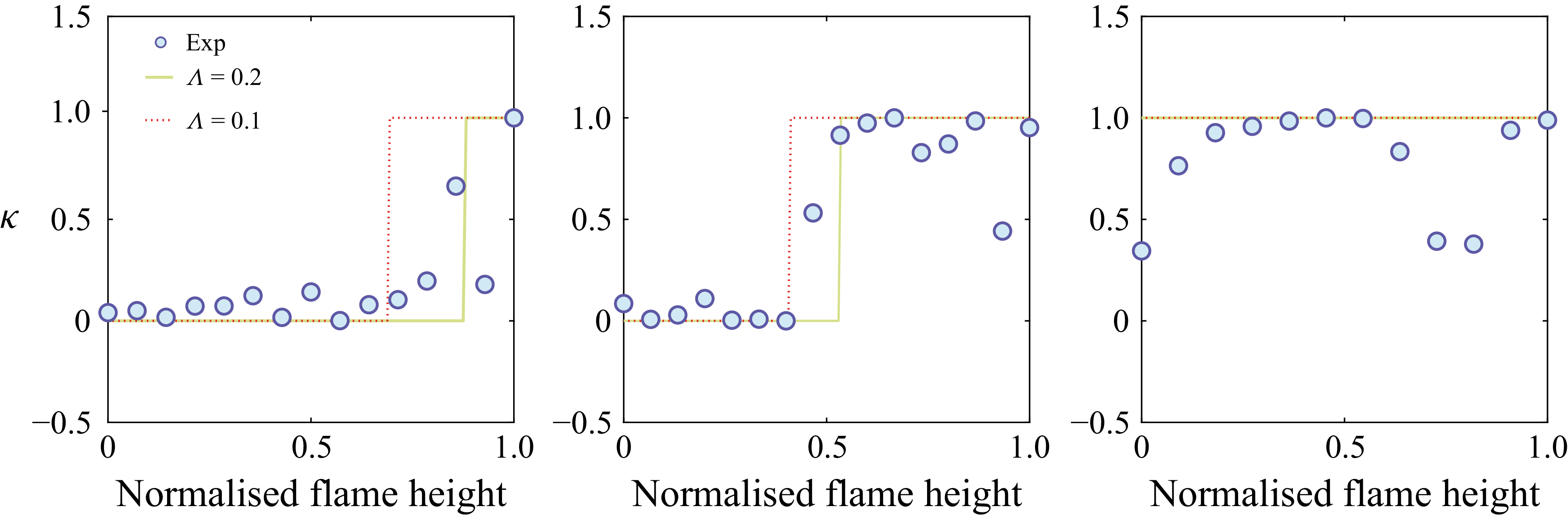
 κ
 f=250
 f=130
 f=50
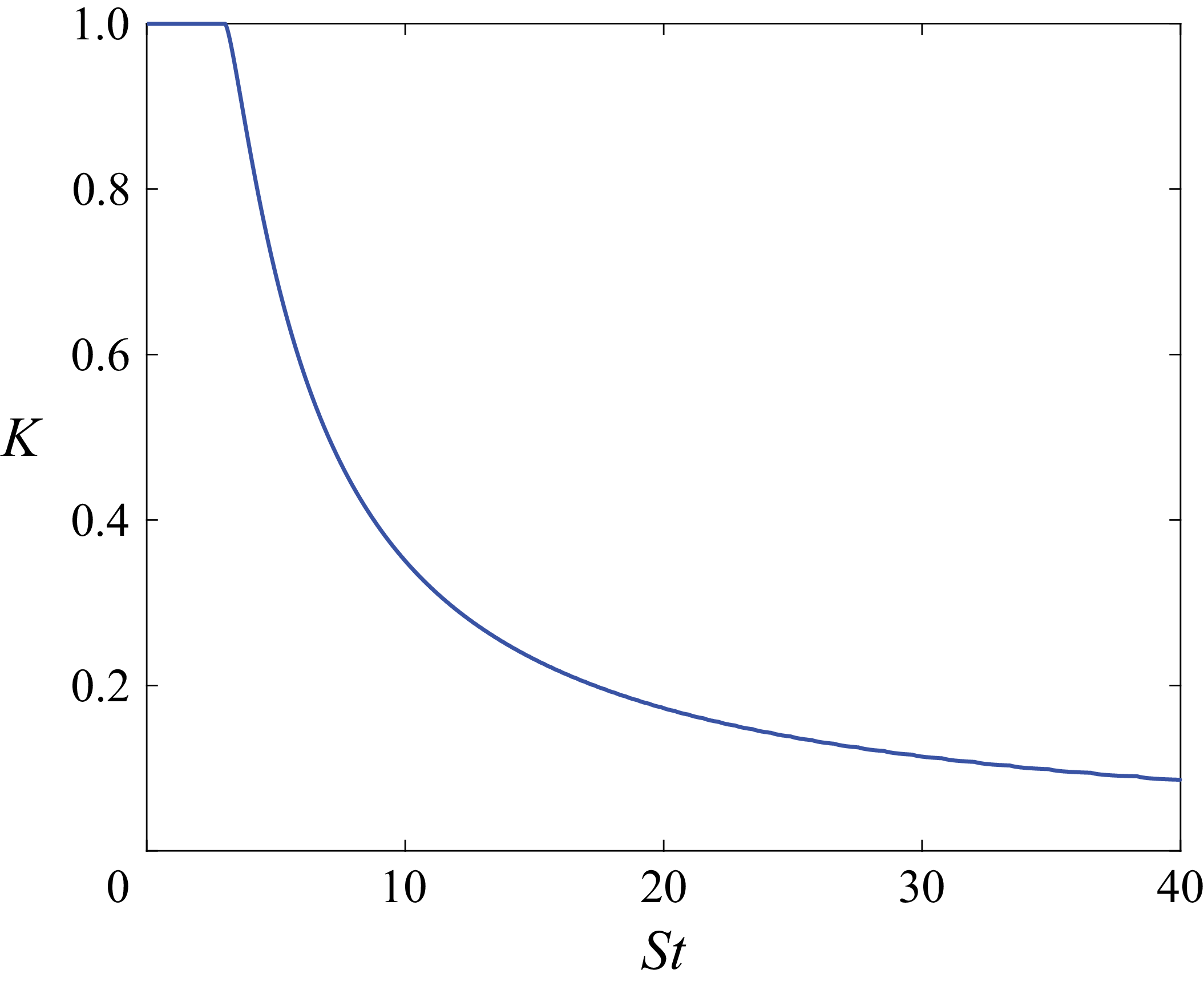
 K
 St
 Λ=0.2
 Ωb=0

 St1
 ϵ1=0.2
 ϵ2=0.1
 δ=π/4
 R=1.6
 R=St2/St1
 cotα=3
 Ωb=0
 N

 St1
 δ=0
 St1=0.1
 R=0.3
 St1=4.7
 R=0.9
 St1=10
 R=0.6
 ϵ1=ϵ2=0.1
 St1=5
 R=1.2
 N
 cotα=3
 R=St2/St1
 Ωb=0

 St1
 St1
 St1=8
 St2=5
 ϵ1=ϵ2=0.2
 cotα=3
 Ωb=0

 St1=1
 St1=5
 St1=9
 HSt1(r)=μI,1,2,2(r)−μI,1,1,1(r)
 R=St2/St1
 cotα=3
 Ωb=0

 Seff,disp(r)
 R=0
 R=2.2
 R=3.6
 R=St2/St1
 ϵ1=ϵ2=0.2
 cotα=3
 Ωb=0

 K=1
 K=0
 K
 St
 −1
 ϵ=0.2

 St1
 ∘
 TV,St1
 PL
 PN
 St2
 ϵ1=0.2
 ϵ2=0.1
 R=St2/St1
 cotα=3
 Ωb=0

 ϵ2=0.2
 ϵ1=0.2
 St1
 St2
 0.9
 St1≈4.3
 St2≈4.3

 St2
 St2=3.5
 ϵ2=0.3
 cotα=3
 St1=2.5
 ϵ1=0.2
 Ωb=0



