




No CrossRef data available.
Article contents
A CENTRAL BANK FOR ALL SEASONS? THE “LOWER INFLATION AT NO COST” PROPOSITION UNDER CONDITIONS OF POLITICAL UNCERTAINTY
Published online by Cambridge University Press: 06 April 2004
Abstract
Recent literature on independent and conservative Central Banks has highlighted the possibility of achieving lower inflation for no increase in the volatility of output—especially when political influences are taken into account. We extend this idea to allow for political uncertainty, where political parties get elected with a probability that may vary over time. We find that it is no longer possible to guarantee lower inflation at no cost at all times. But it is possible to guarantee one or other property if the bank is very conservative or if the governments are always liberal. That implies a conventional inflation–output stability trade-off. However, it is also possible to have conditions in which neither property applies.
Information
- Type
- Research Article
- Information
- Copyright
- © 2004 Cambridge University Press
INTRODUCTION
Conventional theory has it that delegating monetary policy to an independent central bank will deliver lower inflation. However, one of the most remarkable results in this literature is the claim that this lower inflation can also be achieved at no cost in terms of larger output fluctuations. Not all models of central bank independence have this property. For example, Rogoff's (1985) model does not. But the model of Alesina and Gatti (1995) does,1
See also the model in Alesina (1989).
The explanation offered by Alesina and Gatti is that central bank independence eliminates the effect of electoral uncertainty on the cycle.2
Removing those elements by delegating monetary policy to an authority subject to neither electoral nor cyclical concerns would clearly reduce the variability of output as well as reduce inflation. However, what this analysis does not cover is the possibility that increased attention to inflation control may, in itself, increase the natural variability of the economic part of the cycle and hence the overall variability of output. A priori, therefore, one cannot tell which way the trade-off will go and the Alesina–Gatti model does not say. That is what we investigate here, when the probability of different electoral outcomes may vary over time.THE CONSERVATIVE CENTRAL BANKER PROPOSITION
The traditional model for analyzing the effectiveness of monetary discipline and policy credibility is due to Barro and Gordon (1983) and Rogoff (1985). They take a “surprise” supply function

where y denotes output as a deviation from its natural rate, π is inflation (and
is the private sector's expectation of that inflation rate), and
is a random supply shock with mean zero and variance
. This relationship has been justified variously as a new Keynesian Phillips curve
3; or the result of setting wages under conditions of imperfect competition4Rotemberg and Woodford (1998).
See Demertzis et al. (1999).
In this type of model, the central bank chooses monetary policy to minimize the following loss or social welfare function:

where b denotes the relative preference for output stabilization, or aversion to output instability, compared to inflation control.
6Gali and Monacelli (2002) have shown how an objective function such as (2) can be derived from the standard microfoundations of an open-economy macromodel.
denotes the level around which output should be stabilized.
7Notice k=0 is allowed in this analysis. Most models take k>0 because the need for social expenditures implies that some distortionary taxation will be necessary—and those distortions will prevent markets from clearing at their full employment levels. Consequently, k>0 needs to be set to compensate: see Persson and Tabellini (1990) for more detailed arguments.
Substituting (1) into (2) implies that the optimal choice for inflation, under rational expectations for the private sector, is

with
as the inflation bias, and
as the deviation of output from its natural rate. Hence, E(y)=0 and
.
The Conservative Central Bank proposal comes from the observation that social welfare can be increased for everyone if monetary policy can be delegated to an independent central banker whose preferences are more conservative than society as a whole—that is, to a bank that is more inflation averse and has a value of
in (2). However, the bank has to be independent. Its policymakers cannot be removed if their policies conflict with those of the government. In such a case the Bank would follow (3) as the optimal policy rule, but using its own value of
for b. Hence, to maximize social welfare, we need to choose a value
that solves

The first-order conditions for this are

Since the first term of (5) is positive, the solution has to be
as claimed. That solution implies policies that are more inflation averse than society would have chosen for itself. However, they are also welfare improving because the bank's operating parameters become subject to choice ex ante. The institutional environment has therefore become an additional choice variable.
POLITICAL UNCERTAINTY
To compare these “conservative” policies with the outcomes that could be expected in their absence, we must recognize that alternative regimes will produce outcomes that are subject to the preferences of whichever government is in power at the time. Alesina and Gatti (1995) provide a model that analyzes that case.
Suppose there are two competing political parties, D and R, with preferences

and

where
. So, party R is more inflation averse (conservative) and D is more unemployment averse (liberal). Suppose wages and costs are set first, and then there are elections. Suppose party D is expected to win those elections with probability p. Then the party that gains power gets to set monetary policy. That means the private sector must expect, ex ante, an inflation rate of

where, if left to themselves, the two parties would choose
and
by minimizing (6) or (7), subject to (1) but constrained, in each case, by the market's expectations
. This implies

and

We would get (
) with probability p; and (
) with probability 1−p. Hence,

but

are the long-run outcomes. The first term of (11) represents the volatility induced by the electoral cycle. It increases with the differences between the two parties, but vanishes with political certainty: that is, if p=0, or p=1, or k=0. The second term represents the volatility caused by supply shocks, but dampened by the degree of stabilization and altered by the different political preferences for output stability.
These outcomes must be compared to those from our independent central bank with
for b:

and

where
, society's preferred value. So, expected inflation is lower, but output volatility is higher, the smaller is
.
LOWER INFLATION AT NO COST?
Can we get lower inflation on average, and also a lower variability of output, by appointing an independent central bank? Lower average inflation requires

which is always positive since the right of (12) is strictly positive. So
, but small enough, will do it.
Similarly, we can always choose
to provide lower output variability. That happens if we choose
to satisfy

where
is the political “signal to noise” ratio.
8The “signal to noise” ratio g reflects the strength of the policy commitment to income stabilization at a certain level, compared to the size of the likely disturbances in that income.
value above a certain limit; and implies that the variability in output due to changing political preferences has been eliminated, and that the impact of stochastic shocks has been reduced—at least to the extent that the term on the left of (13) is smaller than the second and third terms on the right. However, there is no guarantee that this last condition will hold. It is also entirely possible that the inequality in (13) will hold even though the second and third terms are smaller than
—in which case the stochastic element in the output variability has risen on the appointment of the independent central bank, even though the political influences have been eliminated.
The key question, therefore, is: can we choose
to give both benefits—lower inflation and lower output volatility—at the same time? The problem is that lower inflation requires a smaller
, but lower volatility requires a larger
. However, we can always achieve both outcomes together, for any given value of p, if there is a nonempty interval for
between the upper bound implied by (12) and the lower bound implied by (13). Starting from (12), we can show that this interval exists if

holds, whereas, from (13),

also holds, where A=[1+bD−p(bD−bR)]2. In other words, the term on the right of (14) must be strictly larger than that on the right of (15). Clearly, that cannot be true if p=0, p=1, or if bD=bR. In those cases, there is no
that will achieve both lower inflation and lower output variability. However, in all other cases such an interval exists, and gets larger as g increases, so long as

Hence, a nonzero interval exists for all values of 0<p<1, and for any finite values of k,
, or
.
9However, this window of opportunity will vanish if
, or
, or
, and it will be reduced dramatically (but not to zero) if k becomes small, or
large.
can always be found to give us both outcomes. However, that does not mean that the same value of
will remain valid if the parameters—and p in particular—change around the cycle or with the electoral calender.
It is worth noting that this result only holds because both the political cycle and the supply-side volatility enter the problem in the politically influenced case. Repeating the same analysis when the upper bound on
comes from (12), but the lower bound comes from just the last two terms of (13), shows that the independent and conservative central bank will only generate lower output volatility in the face of stochastic shocks if p<1/2. Conversely, it will only generate less volatility than that induced by the electoral calender if

that is, if k is large and
is small, but
,
,
. These results show that it is the independence of electoral outcomes, not the conservative nature or credibility of the policies per se, that is providing the lower inflation at no cost result. However, it is not a general result. It requires k large enough, or
small enough, and bD−bR large enough for the current value of p. If those quantities were to change over time, in particular if bD−bR or p were to change, then the permitted interval for
and the lower inflation at no cost property would both be lost. That is a problem because the whole point of this analysis is that the chosen value of
should not be changed until the current Banker's term of office expires—and especially not each time a different government appears likely to take office.
ONCE THE BANK IS CHOSEN, WILL IT CONTINUE TO DELIVER LOWER INFLATION AT NO COST?
The problem with the results in Section 4 is that the appropriate value of
is specific to the particular value of p (or, equivalently, to the specific values of bD and bR) which held at the moment the central bank was chosen. If the choice interval for
at that time was relatively narrow (perhaps because bD−bR was small, or p was small), then the chosen
could easily become invalid as the electoral fortunes of each party change. And that means the economy would no longer be getting lower inflation at lower output volatility, compared to what it could be getting with policies appropriate for the new circumstances.
From (12), we can see that we will get lower inflation from the chosen
only if the value of p is such that

For this to make sense, we will require
, so that
. However, (18) also implies that pL>0 only if
. In other words, we can only get lower inflation for all possible values of p if
is chosen. Otherwise we will only get lower inflation when the probability of party D forming a government is greater than pL.
Conversely, we will get lower output variability only if p satisfies (13) for the given
: that is, only for the values of p that satisfy

where

and
if
. This sign pattern means that we are faced with two possible situations, depending on whether
or
. These two cases
10The case of
is ambiguous. It is easy to check that
at p=0 and
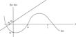
. Hence this case looks like Figure 1 if
, but like Figure 2 otherwise. Since bD>bR, it is relatively easy to have g2 large enough if the political parties diverge strongly or have ambitious targets for the output levels (versus its stabilization).

Case A:
. In this case, a0<0 and the results follow from Figure 1 in which f(p)=0 has one root pF, in the interval [0, 1]. This leads to Proposition 1.
PROPOSITION 1. If
, then we will always have one property (lower inflation), or both properties (lower inflation and lower output variability), depending on whether p is currently below pF or above it. However, we can never have both properties for all values of p.
Proof. See Appendix A.
Comment 1. It is possible to get both properties together if
exactly, if k2 exceeds
sufficiently, and if bD is sufficiently different from bR. However, that is a very special case: Insufficient differences between the political parties, say
, or a nonpartisan central bank (
), or a moderate target for the level of output (k) compared to its natural variance (
), would prevent it. Appendix A contains the details.
Case B:
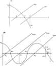
. In this case, a0>0 and f(p)=0 will have either one or three positive roots. Figures 2A and 2B apply accordingly. There are various possible positions for h(p) depending on the value of PL, and hence on the choice of
.

PROPOSITION 2. If f(p)=0 has a single positive root, Figure 2A, then either one or the other of the desired properties will always hold—lower inflation if p>pL, or lower output variability if p<pF. It is also possible that both properties will hold simultaneously if
.
Proof. See Appendix A.
Comment 2. Again we can never get both properties for all values of p. However, there is one, possibly small, interval of values for p where both properties apply, and there is no interval where neither property applies.
PROPOSITION 3. If f(p)=0 has three positive roots, Figure 2B, then there will always be some interval where both properties (lower inflation and lower output volatility) hold. However, there will also be intervals for p where only one of the two properties holds (lower output volatility when
or pL3>pF2, but lower inflation when
or pL2<pF2). These different values of pL1, pL2, and pL3 reflect three possible choices of
[and hence of h(p)]. Moreover, there is also always one interval, (pF1, pL2), if
is chosen to yield pL2, or (pF1, pF2) if
is chosen to yield pL3, in which neither property holds, although
has been correctly chosen.
Proof. See Appendix A.
Comment 3. The upshot of our results so far is that there will always be intervals for p where both lower inflation and lower output volatility hold, but no case where both properties hold for all values of p. Conversely, unless we can find some mechanism by which the central bank can be made both independent and to rule out Proposition 3 altogether by imposing a suitable choice for
, there will also be intervals for p where neither property is achieved. In between these extremes, there will always be times when only one or the other of the two properties holds.
PROPOSITION 4. It is only possible to rule out Proposition 3 in the case where all possible governments are very liberal, and where the central bank is permitted to be no more liberal than the most conservative of the possible governments. That occurs when governments are either “target liberal” (g2 is large) or “weight liberal” such that
is large enough and inequality (A.4) applies. However, Proposition 3 may also be ruled out if the central bank is very conservative in itself
, so that Proposition 1 applies.
Proof. See Appendix A, Case C.
Comment 4. All the results so far assume
has been verified to lie within the nonzero interval implied by the lower bound in (15) and the upper bound in (14). If it does,
can be said to be “correctly chosen” for current value of p. However, if it does not, perhaps because it has been evaluated for some past value of p, or because it has proved too hard to obtain accurate measures of bD or bR from the political parties, then it will also be possible to get intervals p1L−pF where neither property holds in Figure 2A; and also no interval where both properties apply (Appendix A). So, to be able to rely on the results derived in Propositions 1 and 2, we not only have to impose sufficient conservatism on the central bank, but also ensure that the
in question has been correctly chosen. Section 6 shows what will be risked if this is not done.
Postscript. Appendix B computes the social welfare outcomes for each of the policy strategies available here: for full commitment when the true value of b is known (or using b=0, if it is not); for the conservative central banker solution with either
or an approximately optimal
to satisfy (5); and for the political economy solution where the central bank's policies are chosen by compromise to reproduce (9)–(11) for the value of p at the moment of the central bank's appointment. These results show that:
- An optimally conservative central bank will choose bounded away from zero, and from below if is small, b is small, or k is large.
- The conservative central banker will always delivers smaller welfare losses than full commitment using b=0, unless is large and k2 is small. However, the differences are small if the true value of b is small, or if is set small.
- The optimally conservative central bank will deliver smaller losses than full commitment with the true value of b, unless is very small. Again, however, the differences are small if the true b is small.
- The political economy compromise is always worse than any conservative central bank.
These results are included to provide a benchmark for the conservative-central-banker and political-economy solutions. They make the point that a conservative central banker may be a convenient way of achieving optimal outcomes when full commitment is not available. However, it may not always be possible to achieve such outcomes, for example, if
is small, and it may not matter much if the true b is small. Thus, these results also make the point that getting “lower inflation at no cost” may not be a particularly important property. Such a property may not be optimal and may not be attained when the electoral probabilities can shift significantly from those that held when the current central bank was appointed. Better to stick with a solution with much lower inflation across all likely electoral outcomes, or one with lower output volatility, even if the other property is made a little worse.
THE PROBABILITY OF GETTING LOWER INFLATION AT NO COST
Finally, if we are able to make specific assumptions about the probability function that governs the chance that party D wins each election, we can compute the probability or proportion of time spent with lower inflation, or with lower output variability, or with both properties, when
is correctly chosen. Conversely, if
takes an inappropriate value, we can compute the proportion of time spent without one or the other property, or with neither of them.
Uniformly Distributed Probabilities
If we take probability that party D wins the next election to be distributed uniformly over the unit interval, as Alesina and Gatti (1995) do, then we will get lower inflation only 1−pL of the time in the long run (assuming
). Similarly, if f(p)=0 is constructed to have a single positive root, then we will have lower output volatility pF of the time (where pF is that root). If
, then we get lower volatility all the time.
Tables 1 and 2 summarize the results of three constructed examples, to show the proportions of time spent with lower inflation, lower output variability, or with both properties. Examples 1 and 3 use a correctly chosen value of
, and Example 3 is the numerical example originally used by Alesina and Gatti to demonstrate the advantage of delegating monetary policy to an independent central bank. Example 2 shows what can happen when
is incorrectly chosen11
Following (18),
would be necessary to get lower inflation at no cost in this case.
could exist such that at least one of the two desired properties holds all the time. However, as we pointed out in Section 5, some of those parameters (bD, bR, and k) are under the policymakers' control. So this situation could be avoided with sufficiently astute policymakers. It is interesting to speculate whether the political parties would also learn to adjust bD or bR in order not to be seen to be offering policy preferences that could predictably lead to periods where neither lower inflation nor lower volatility would be achieved.


Table 2, which is derived from the pL and pF figures reported in Table 1, shows that the conservative central bank—under reasonable values for the preference and output variance parameters—would do a pretty good job of providing lower inflation than a dependent or politically influenced central bank. It would also do a pretty good job of providing lower variability in output. In most cases, it can provide one or the other property alone for 50–75% of the time.
The striking result, however, is the fact that the conservative central bank seldom achieves both properties together—that is, low inflation at no cost. In fact, this occurs just 6% of the time in Examples 1 and 3, and never in Example 2. On the other hand, it achieves neither property rather more often if
is poorly chosen: 26% of the time in Example 2.
These results are significant because they show that the advantages of having a conservative and independent central bank are sensitive to small shifts in the underlying political or economic conditions. For example, a small shift of 6 percentage points in the probability of party D getting elected can destroy those advantages altogether, and put us back into a position where we have to trade off lower inflation for greater output stability in the traditional manner (Examples 1 and 3). In addition, similar-sized shifts in the public's preference for more conservative policies (i.e., toward party R) from a position of neutrality (p=0.5), can cost us both properties for significant periods of time: 26% of the time in Example 2.
Hence the disadvantage of an independent and conservative central bank is that, once chosen, it is hard to change and may go on delivering unfavorable policies long after the economic and political circumstances of its birth have changed. It may therefore turn out to have been a bank for particular circumstances, rather than a “bank for all seasons.”
Normally Distributed Probabilities
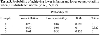
Table 3 recomputes the proportions reported in Table 2, for the same four examples, when the probability of party D being elected is normally distributed, N(0.5, 0.2). The interval
then contains 95% of the potential realizations of p. The results, however, are not very different from those in Table 2. The probability of getting lower inflation at no cost in output stability increases somewhat, but still reaches only 10–12%. However, the proportion of time spent with neither property when
is poorly chosen also increases, to around 33%. So, our conclusions about the low-inflation-at-no-cost result being very sensitive to small shifts in the political and economic circumstances remain. In fact, the lower-inflation-at-no-cost property will hold only for a small minority of the time.

CONCLUSION
The conventional wisdom that an independent central bank can achieve “lower inflation at no cost” is extremely fragile under conditions of political uncertainty.
It is always possible for such a bank to get both lower inflation and lower output volatility some of the time, that is, across different political and economic circumstances, and across different electoral outcomes. However, it is never possible to have both of those properties all the time, except in a very special range of circumstances involving a totally partisan central bank, highly differentiated political parties, and relatively small output shocks. In more conventional circumstances, the time actually spent with both properties may be quite small in relation to the time spent with only one of them.
That said, a central bank designed as a political compromise (i.e.,
) carries the danger that it will actually achieve neither of those two properties for a significant part of the time. This danger can only be ruled out by making the bank extremely conservative
, or by electing only liberal governments. In those cases the danger that we get neither property may be ruled out, but at some considerable cost to the probability of getting both properties. So, as is so often the case, there is no free lunch.
On the other hand these results have all been derived in the absence of fiscal policy. The fact that better results may be obtained when liberal governments are elected suggests that fiscal policies may be an important component in getting lower inflation at no cost, and lower welfare losses at the same time. To examine the robustness of these results when the fiscal–monetary policy mix may change would be the next step for this research.
APPENDIX A
The proofs for Section 5. Note that there are only two time periods in all these results: “then,” when the central bank was appointed or given its mandate; and “now,” when the value of p may have shifted. The results are therefore all comparative static.
Case A:
. The consequence of having both a0 and a3 negative is that f(p)=0 in Figure 1 must have two positive roots and one of them in the interval [0, 1]. We know that because the results of Section 4 showed that there was always at least one value of
such that both f(p) and h(p) were positive, and an interval around that value such that
could be chosen to deliver both properties. However, if there is one such root and a0<0, then there must be two positive roots in total. Hence Figure 1 is relatively straightforward. We will always have either one property (i.e., lower inflation) or both properties (lower inflation and lower output variability), depending on whether p is currently below pF or above it. However, we will never have both properties for all values of p, except in the unlikely event that
exactly, and g2 is large enough to make
at p=0, and
.12
The first two of these conditions is needed to ensure
, and
at p=0; and the third is needed to ensure
. Those conditions ensure that the lower output volatility property holds at both ends of the unit interval for p.
, would be enough to ensure that both properties cannot hold for all values of p. Also, the central bank has to be seen as partisan
. And there has to be an ambitious value for g, not just output shocks per se.
Case B:
. The situation is now more complicated. Since a0>0, f(p)=0 must now have either one or three positive roots: Figure 2A or 2B, respectively, where there are various possible positions for h(p), depending on pL and the choice of
. There are also two possible results at the right-hand end of panel (B), depending on whether
or f(1)<0: that is, on whether
is positive or negative.
If we have the single positive root case, Figure 2A, it is obvious that either one or the other of the desired properties will always hold—lower inflation if p>pL, or lower output volatility if p<pF, or both of them if
. That is the situation if h(p) reflects the current choice of
. If we raise the value of
such that h(p)1, and hence p1L and f(p1L)<0 now apply, then there is an interval p1L−pF where neither property holds, and no interval where both properties hold. However, that contradicts the results of Section 4, which showed that, for any p, there is always some value of
that can be chosen such that both properties will hold. Consequently, if
is correctly chosen, we cannot have the situation represented by h(p)1 and p1L in Figure 2A.
If there are three positive roots however (Figure 2B), then there is always an interval for p where both properties hold so long as pL3 is not greater than pF3 (i.e., as long as
is correctly chosen). However, there will always be an area where only one of the two properties holds (i.e., lower output volatility when
, and lower inflation when
), if
is correctly chosen such that pL1<pF1. In fact, we can consider three alternative choices of
, yielding pL1 or pL2 or pL3, respectively. These two areas will then continue to exist for all
and
.
In addition, there will also be areas with lower inflation only if
is chosen to yield pL2 such that pL2<pF2, or lower output volatility only if
yields pL3>pF2. However, in the two latter cases, there will also be an interval (pF1, pL2), or (pF1, pF2) if
implies pL3, in which neither property holds even though
has been correctly chosen. That is a new result. It says that, even if
is correctly chosen, there is a significant possibility that there will be intervals for p (and hence periods of time) where neither lower inflation nor lower output volatility is achieved. The only way to rule that possibility out is to rule out values of
that generate pL2 or pL3, or to rule out the three positive roots case. The former is difficult because it is equivalent to ensuring that we have
, where
is the smallest positive root for
in
and
is (18) with
inserted for
. To ensure that, we would have to solve a fifth order polynominal in
. It is easier to proceed with the strategy of ruling out the three positive roots.
Case C: Ruling Out the Three Positive Roots. We need now to rule out the possibility that we get neither lower inflation nor lower output variability. The easiest way to do that is to choose
so that f(p)=0 has one positive root and two complex or two negative roots. Doing that will effectively return us to Figure 2A, where we get one or the other of the two properties all the time, and both of them some of the time. However, we no longer risk getting neither of them at some values of p.
To rule out three positive roots, we use Descartes's “rule of signs”: The number of positive rule roots to f(p)=0 is the number of variations in sign in the sequence

when
, or a number less than that by an even integer.
13Demidovich and Maron (1973, pp. 178–179).
), however, there will be three variations in sign and we have to use Hua's corollary [Demidovich and Maron (1973)]: that is, if, for some
in (A.1),

then (19) has at least one pair of complex roots. If we evaluate (19) at g2=0, we get a3, a1<0 and a2, a0>0. So, it is a matter of direct calculation to establish whether either
or
in each case. Take the former case. Using (19) and g2=0, we can write

Leting
, and collecting all nonzero terms remaining in (A.3) together, we have

This will be negative, implying (19) has one pair of complex roots, if

This last inequality may be satisfied by larger values of bD and bR, for example, bD=1, bR=3/4, and
, that is, by relatively liberal governments and a central bank that is no more liberal than the most conservative of the possible governments.
Hence it is possible to rule out the case in which neither lower inflation nor lower output volatility is achieved when
is correctly chosen—but only where governments and the central bank are relatively liberal [either g2 is large, or
and (A.4) applies], or where the central bank is very conservative
.
APPENDIX B
In this appendix we compute the social welfare losses under the three different policy strategies: (i) the full commitment solution (with either the true value of b or b=0); (ii) the conservative central banker solution [with either
or
to satisfy (5)]; and (iii) the political economy solution where the central bank's policies are chosen by (9) and (10) for any given
. In the first two solutions, the central bank is independent. In the third, it is still independent, but is obliged to follow the preferences imposed by the government that appoints it. In all three cases, the welfare losses are computed from (2) where “b” is known and represents the true preferences of society as a whole. That implies that we can rewrite (2) as follows:

since E(y)=0 in all three cases.
Strategy (i). Full commitment, with
. Equation (3) applies and we get

However, full commitment with b=0 in the decision rule, but not in the social welfare function, would have implied

Strategy (ii). A conservative central banker, with
. The policy outcomes in the last paragraph of Section 3 now apply. Hence,

and the full commitment (
) version of this yields (B.3) again. Notice that (B.4) implies

which is certainly positive for all
, and which is certainly negative (
) at
. Moreover, the second derivative is easily checked to be positive for all values of
. Therefore, assuming the central bank to be conservative relative to the population, we have a unique minimum to (B.4) and at (5) of the main text. Also, although a closed-form solution for the optimal value of
does not exist, we can obtain a good approximation by linear interpolation:

or
if
is not very large. Hence,
is never zero, given b>0 and
. In fact,
.
Strategy (iii). A political-economy central bank. We first take p to be fixed at the moment the central bank's governing council is appointed, and then consider what happens if p subsequently varies. Using (9), (10), and (11), we get

Hence,
if
, and something larger than that for
.
Comparison (i). A conservative central banker over full commitment (with either
or b=0 in the policy rules). Using (B.4) and (B.3), the conservative central banker will deliver better results if

is positive. That is likely, but not guaranteed for every
—especially if
is large and k2 is small. It certainly holds if
are both small, unless
is very large. However, the gains from the conservative central bank are small if
is small.
Comparison (ii). An optimal conservative central banker over full commitment
. Using
and (B.2), the conservative central banker delivers better results if

is positive. That will hold unless
is very small (in which case
is a poor approximation anyway). However, the gains are not very important if the true value of b is rather small: that is, if the population itself is fairly conservative.
Comparison (iii). The political-economy central bank vs. a conservative central banker
. Comparing (B.4) with (B.7), the political-economy central bank gives worse outcomes if the following expressions are positive:

which is the term in k2; and

which is the term in
. The term in k2 is certainly positive at p=0 if
, or if
. The term in
is likewise positive at p=0 if
and
. Given those restrictions, meaning only that the central bank is conservative relative to the population as a whole, and that the more conservative politicians are never more than twice as liberal as the central bank, then it is easy to check that the term in k2 is increasing in p, for all
as long as
, and that the term in
is likewise increasing in p as long as bR is somewhat smaller than b: formally,

where bR<bD. Under these conditions, the political-economy central bank will always deliver worse results than the conservative central bank, whether there is a “lower inflation at no cost” property or not.
References
Alesina A.
1989
Politics and business cycles in industrial democracies.
Economic Policy
8,
55
98.Google Scholar
Alesina A. &
R. Gatti
1995
Independent central banks: Low inflation at no cost.
American Economic Review
85,
196
200.Google Scholar
Alesina A. &
L. Summers
1993
Central bank independence and macroeconomic performance: Some comparative evidence.
Journal of Money Credit and Banking
251,
151
162.Google Scholar
Barro R. &
D. Gordon
1983
A positive theory of monetary policy in a natural rate model.
Journal of Political Economy
91,
589
610.Google Scholar
Cuckierman A.
1996
The Economics of Central Banking. Discussion paper 9631,
Tilburg University.
Demertzis M.,
A. Hughes Hallett &
N. Viegi
1999
An Independent Central Bank Faced with Elected Governments: A Political Economy Conflict. Discussion paper 2219,
Centre for Economic Policy Research.
Demidovich B. &
I. Maron
1973
Computational Mathematics,
Moscow:
Mir.
Eijffinger S.,
E. Schalling &
M. Hoeberichts
1998
Central bank independence: A sensitivity analysis.
European Journal of Political Economy
14,
73
88.Google Scholar
Gali J.,
M. Gertler &
J. Lopez-Salido
2001
European inflation dynamics.
European Economic Review
45,
1237
1270.Google Scholar
Gali J. &
T. Monacelli
2002
Monetary Policy and Exchange Rate Volatility in a Small Open Economy. Discussion paper 3346,
Centre for Economic Policy Research.
Mangano G.
1998
Measuring central bank independence: A tale of subjectivity and its consequences.
Oxford Economic Papers
50,
468
492.Google Scholar
Persson T. &
G. Tabellini
1990
Macroeconomic Policy, Credibility and Politics.
Amsterdam:
Harwood Academic.
Posen A.
1998
Central bank independence and disinflation credibility: A missing link.
Oxford Economic Papers
50,
335
359.Google Scholar
Roberts J.M.
1995
New Keynesian Economics and the Phillips Curve
Journal of Money Credit and Banking
27,
439
446.Google Scholar
Rogoff K.
1985
The optimal degree of commitment to a monetary target.
Quarterly Journal of Economics
100,
1169
1190.Google Scholar
Rotemberg J. &
M. Woodford
1998
An Optimisation Based Econometric Framework for the Evaluation of Monetary Policy.
NBER technical paper 233.
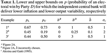
Lower and upper bounds on p (probability of an electoral win by Party D) for which the independent central bank will deliver lower inflation and lower output variability, respectively
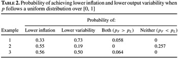
Probability of achieving lower inflation and lower output variability when p follows a uniform distribution over [0, 1]
Probability of achieving lower inflation and lower output volatility when p is distributed normally: N(0.5, 0.2)
 You have
Access
- 2
- Cited by