


1. Introduction
Telematics has become a cornerstone data source in auto insurance, capturing high-frequency GPS and on-board-sensor signals such as speed profiles, acceleration/braking, cornering, and time-of-day. This differs from traditional rating variables such as age, vehicle, and prior claims, which act largely as proxies for risk rather than direct measures of driving behavior. The availability of rich telemetry enables usage-based insurance (UBI) models, supports more granular and behavior-based ratemaking, provides dynamic feedback that can promote safer driving, and delivers operational benefits in underwriting and claims management (Boucher and Turcotte, Reference Boucher and Turcotte2013). Prior studies investigate how GPS/behavioral features augment pricing and exposure measurement (Guillen et al., Reference Guillen, Nielsen, Ayuso and Pérez-Marín2019), summarize the telematics data landscape and cleaning/privacy issues (Gao et al., Reference Gao, Meng and Wüthrich2022a), and show benefits from behavior-based scoring and program design (Winlaw et al., Reference Winlaw, Steiner, MacKay and Hilal2019). Recent reviews synthesize these impacts across research and practice (Boylan et al., Reference Boylan, Meyer and Chen2024; Chauhan and Yadav, Reference Chauhan and Yadav2024).
A growing actuarial literature asks what and how to learn from telematics information. Ayuso et al. (Reference Ayuso, Guillen and Nielsen2019) established mileage and related exposure metrics as predictive for claim frequency. A widely used tool is the speed-acceleration heatmap, which captures time spent across speed-acceleration cells and yields features for pricing models (Gao and Wüthrich, Reference Gao and Wüthrich2018). Subsequent work shows that these telematics features improve claim-frequency prediction in GLM/GBM-type frameworks (Gao et al., Reference Gao, Meng and Wüthrich2019, Reference Gao, Wang and Wüthrich2022b). Surveys synthesize work on representations and algorithms for ratemaking and risk scoring, noting improvements in performance alongside data-processing challenges (Gao et al., Reference Gao, Meng and Wüthrich2022a; Boylan et al., Reference Boylan, Meyer and Chen2024).
A practical limitation is that telematics is not available for every policyholder. In many portfolios, there are two groups: (1) a large set with only traditional variables and (2) a smaller set with both traditional and telematics variables, reflecting opt-in and program design. Industry reports highlight privacy concerns and uneven adoption that limit participation in telematics programs. Legal and regulatory discussions also note resistance to in-car tracking, with implications for pricing and consumer welfare (Ben-Shahar, Reference Ben-Shahar2023). These frictions can induce selection effects (e.g., safer drivers opting in), so analyses that drop telematics or use only the telematics subset risk inefficiency or bias; recent actuarial work proposes calibration-based integration to combine the two groups while addressing selection (Peiris et al., Reference Peiris, Jeong, Kim and Lee2024).
In this article, we develop a predictive framework that leverages the two-view structure of car insurance data – one view with traditional rating variables and another with additional telematics features – under heterogeneous availability. In machine learning, multi-view learning treats each coherent source of information as a “view” and aims to exploit the complementary information among different views to improve learning performance (Zhao et al., Reference Zhao, Xie, Xu and Sun2017). A central design choice in multi-view learning is how information from different views is integrated or fused (Yu et al., Reference Yu, Dong, Yu, Yang, Fan and Chen2025). Fusion strategies are commonly categorized according to the stage at which information sources are combined: early fusion combines variables from different views into a single feature set, intermediate fusion combines learned representations, and late fusion combines outputs or predictions from view-specific models (Stahlschmidt et al., Reference Stahlschmidt, Ulfenborg and Synnergren2022; Guarrasi et al., Reference Guarrasi, Aksu, Caruso, Di Feola, Rofena, Ruffini and Soda2024).
Early fusion is not well aligned with this data structure because the two views have unequal availability. Traditional rating variables are available for all policyholders, but telematics variables are available only for UBI participants. Combining the two views at the feature level would therefore force the analysis to rely on the smaller complete-case subset or require additional modeling assumptions for the missing telematics view. Intermediate fusion has a similar drawback: although the fusion occurs after representation learning rather than at the raw-feature level, the joint representation would still have to be learned mainly from policyholders for whom both views are observed. We therefore adopt late fusion, which allows separate models to be trained using the data available for each view and combines their predictions at the final stage.
Our framework builds on the literature on multi-view learning by applying multi-view ensemble principles to actuarial modeling, where telematics data may be partially available across policyholders and heterogeneous in quality. We train separate learners in each view and then combine them at the prediction stage. For weighting the view-level predictions, we use Bayesian model averaging (BMA). BMA treats each candidate model (here, each view-specific model or their combinations) as a component and weights predictions by their posterior model probabilities, providing a coherent way to account for model uncertainty while yielding full predictive distributions and standard uncertainty quantification (Hoeting et al., Reference Hoeting, Madigan, Raftery and Volinsky1999; Claeskens and Hjort, Reference Claeskens and Hjort2008). Thus, in our framework, BMA serves as the specific multi-view learning mechanism: it combines traditional and telematics-based predictions through posterior model weights while preserving interpretability and leveraging information from both data sources.
BMA has been effective in diverse areas: post-processing ensemble forecasts for temperature/precipitation (Raftery et al., Reference Raftery, Gneiting, Balabdaoui and Polakowski2005; Sloughter et al., Reference Sloughter, Raftery, Gneiting and Fraley2007), cross-country growth regressions (Fernández et al., Reference Fernández, Ley and Steel2001), and gene-selection/classification from microarrays (Yeung et al., Reference Yeung, Bumgarner and Raftery2005). Within insurance, applications remain limited and largely outside telematics ratemaking. For example, BMA has been applied to factor-collapsing in claim modeling (Hu et al., Reference Hu, O’Hagan and Murphy2018) and to actuarial reserving via heteroscedastic BMA approaches (Jessup et al., Reference Jessup, Mailhot and Pigeon2025). To the best of our knowledge, multi-view learning has not been used to integrate traditional and telematics views for auto insurance data.
This paper makes three main contributions. First, we formulate the heterogeneous availability of traditional and telematics variables as a multi-view learning problem, where conventional rating variables and telematics variables are treated as distinct but complementary views. Second, we use BMA in a novel way as a multi-view learning mechanism for combining view-specific models trained on different data sources, rather than only as a tool for averaging competing models trained on the same dataset. Third, we show that the resulting BMA weights provide an interpretable diagnostic of how traditional and telematics-based models contribute to prediction. We assess performance using synthetic scenarios that emulate heterogeneous telematics availability and selection. Our empirical study shows the efficiency and flexibility of the proposed method in the prediction of both claim frequency and claim severity.
The remainder of the paper is organized as follows. Section 2 describes the unique structure of auto insurance data for predictive modeling. Section 3 presents the details of the BMA framework for multi-view ensembles. In Section 4, we demonstrate the effectiveness of the proposed approach over individual models using synthetic data for both claim frequnecy and claim severity. Section 5 concludes the paper.
2. Data structure
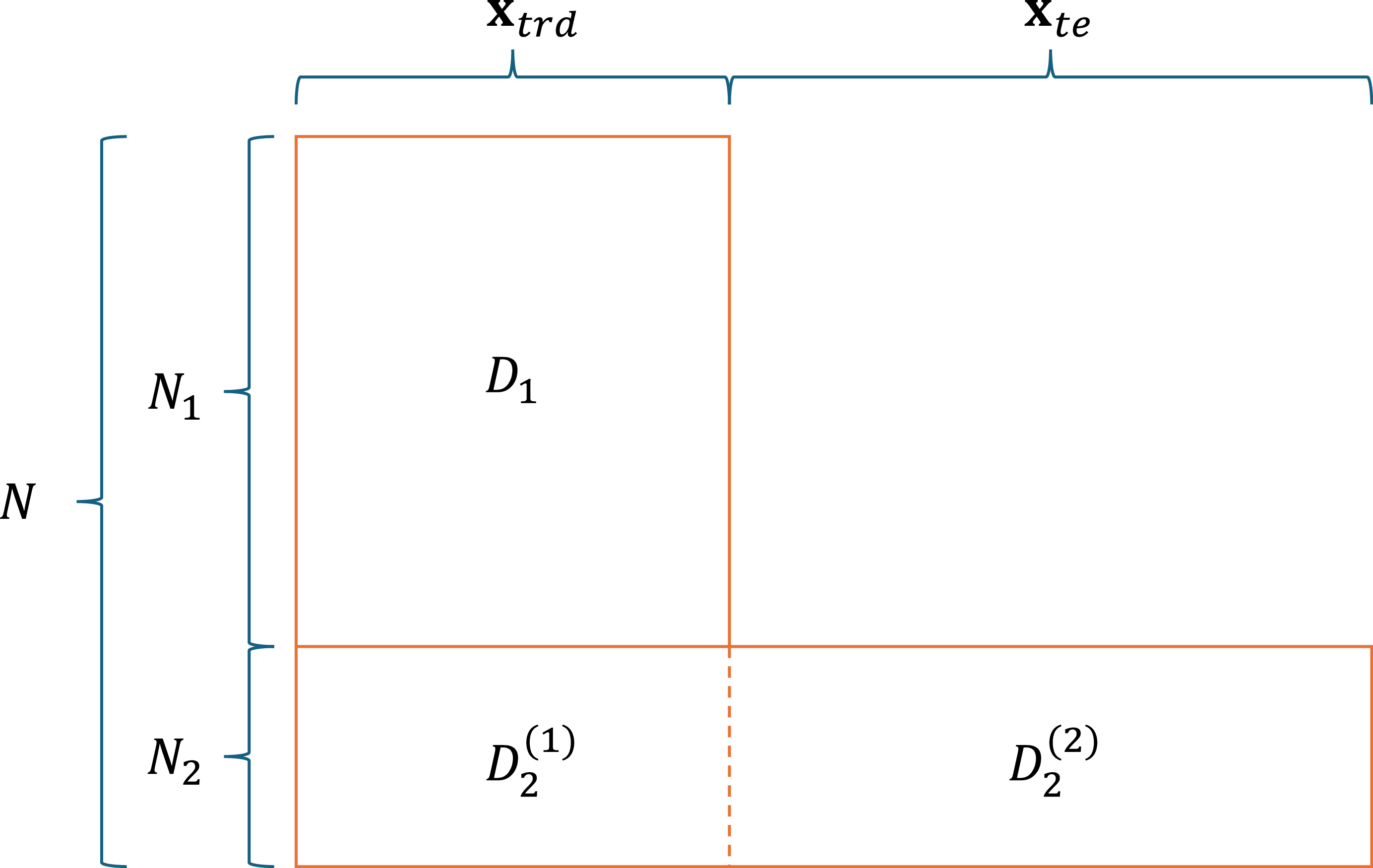
We assume that the auto insurance dataset is split into two groups depending on the presence of telematics features. Subgroup
 $D_1$
contains information of non-UBI insureds comprising solely traditional features, represented by
 $\mathbf{x}_{trd}$
, while subgroup
 $D_2$
consists of UBI insureds including both their traditional features
 $\mathbf{x}_{trd}$
and telematics features, represented by
 $\mathbf{x}_{te}$
. Furthermore, we denote
 $N_j$
as the number of observations in subgroup
 $D_j$
,
 $j = 1, 2$
. Consequently, traditional features
 $\mathbf{x}_{trd}$
are present in all
 $N=N_1+N_2$
policyholders, whereas telematics features are exclusive to
 $N_2$
policyholders. Figure 1 illustrates the organization of the data.
The data structure with two distinct data sources.

There are two characteristics that are worth noting for this unique type of data structure. First, there are typically much fewer UBI subscribers than non-subscribers. Although UBI contracts have been available to policyholders for over two decades, its adoption has remained limited. According to Holzapfel et al. (Reference Holzapfel, Peter and Richter2024), UBI’s market share in the auto insurance sector is roughly 5%. Therefore, it naturally follows that
 $N_1 \gt \gt N_2$
, although the ratio
 $N_1/N_2$
may decrease over time as more policyholders subscribe UBI contracts.
Another key aspect of the data is the potential heterogeneity between policyholders in
 $D_1$
and
 $D_2$
. As Peiris et al. (Reference Peiris, Jeong, Kim and Lee2024) points out, participation in a telematics program is unlikely to be random, and policyholders who opt into UBI contracts may differ systematically from those who do not. Previous studies indicate that lower-risk drivers are more inclined to adopt telematics-based insurance to obtain potential premium reductions (Denuit et al., Reference Denuit, Guillen and Trufin2019; Duval et al., Reference Duval, Boucher and Pigeon2023), whereas higher-risk drivers may be less willing to undergo monitoring. Information asymmetry can further amplify this tendency, as safer drivers are generally more willing to disclose their driving behavior, resulting in favorable selection in the telematics sample (Cohen and Siegelman, Reference Cohen and Siegelman2010). Privacy concerns also contribute: many policyholders remain reluctant to share detailed driving information, which introduces additional selection effects (Duri et al., Reference Duri, Gruteser, Liu, Moskowitz, Perez, Singh and Tang2002; Milanović et al., 2020). As a result, policyholders in the two data groups may differ in their demographic or behavioral characteristics.
This issue is also related to counterfactual reasoning. For non-UBI policyholders, the telematics variables that would have been observed had they participated in a UBI program are unobserved counterfactual quantities. If participation is selective, the distribution of these counterfactual telematics variables may differ from the observed telematics distribution among UBI participants. This highlights a fundamental statistical challenge in telematics modeling: the observed telematics sample may not represent the telematics behavior that would be observed in the full portfolio under universal participation (Winship and Morgan, Reference Winship and Morgan1999; Morgan and Winship, Reference Morgan and Winship2015). In this paper, we do not attempt to identify this full counterfactual distribution; instead, we account for this concern through selection scenarios in which the telematics group differs systematically from the broader portfolio.
3. Proposed method
3.1. BMA for predictive model ensemble
Given the unique structure of the data due to the limitedly available telematics information, we address the predictive modeling problem by employing multi-view ensemble learning (Zhao et al., Reference Zhao, Xie, Xu and Sun2017). The concept of “multi-view” assumes that telematics information offers a distinct and potentially valuable perspective compared to traditional feature information. Multi-view learning has been applied to various machine learning challenges, including dimension reduction, semi-supervised learning, and clustering. However, our focus is to adapt the multi-view approach within an ensemble learning context. We start by training individual models from individual views and then aim to integrate these models into an effective ensemble framework through BMA. In this sense, multi-view ensemble learning describes the overall modeling structure, while BMA serves as the aggregation method used to combine the predictions from the view-specific models. This section elaborates on the use of the BMA ensemble to facilitate the unique structure of the data described in Section 2.
BMA is a well-established statistical model that integrates predictions from multiple models and quantifies model uncertainty using an ensemble posterior probability density function. Rather than depending on a single best model, BMA combines the predictions of various models via a weighted average.
Let Y denote the response variable to be predicted, and
 $M_1,\ldots,M_K$
denote the candidate predictive models. Under the Bayesian framework, the predictive distribution of a general predictive formula for Y could be obtained by averaging the model-specific predictive distributions, that is,
 \begin{align*}p(y)= \sum_{j=1}^{K} p(M_j) \ p(y \mid M_j), \end{align*}
where p(y) is the predictive distribution of Y and
 $p(y \mid M_j)$
is the predictive distribution of Y under model
 $M_j$
. Note that depending on whether Y is a continuous or discrete random variable, the predictive distributions p(y) and
 $p(y\mid M_j)$
can be interpreted as its probability density function or probability mass function. Here,
 $p(M_j)$
denotes the posterior probability assigned to model
 $M_j$
. The posterior model probabilities are nonnegative and sum up to 1 and can therefore be interpreted as model weights.
Once the individual models are fitted, each model
 $M_j$
produces a prediction
 $\widehat{y}_{j}$
for an observation, and the BMA ensemble combines the predictive distributions associated with these model-specific predictions. To clearly reflect the conditional distribution on
 $\widehat{y}_{j}$
, we denote the predictive distribution
 $p(y \mid M_j)$
as
 $f_j(y \mid \widehat{y}_{j})$
. The specific choices of
 $f_j(y \mid \widehat{y}_j)$
used in our numerical study are described in Section 4.
Hence, we obtain a more specific BMA predictive distribution:
 \begin{equation}p_w(y \mid \widehat{y}_{1},\ldots,\widehat{y}_{K})=\sum_{j=1}^{K}w_j\ f_j(y \mid \widehat{y}_{j}),\end{equation}
where
 $w_j=p(M_j)$
is the BMA weight assigned to model
 $M_j$
. Here, we denote the weight vector
 $w\,:\!= \,(w_1,\ldots, w_K)$
satisfying
 $w_j\ge 0$
and
 $\sum_{j=1}^{K}w_j=1$
. Note that, in our multi-view setting, the candidate models are not necessarily trained on the same dataset. In this formulation, the weights are estimated from the validation data and reflect the relative predictive support for the candidate models. Then, the mean, that is, the conditional expectation of Y, becomes
 \begin{equation}\mu = E({Y}\mid \widehat{y}_1,\ldots,\widehat{y}_K) = \sum_{j=1}^{K} w_j E_j({Y}\mid \widehat{y}_j).\end{equation}
Once the weights
 ${w}_j$
’s are estimated, the BMA ensemble prediction is obtained by
 \begin{align*}\widehat{y}=\sum_{j=1}^K \widehat{w}_j\ \widehat{y}_j. \end{align*}
The estimation of the weights
 $\widehat{w}_j$
’s is described below.
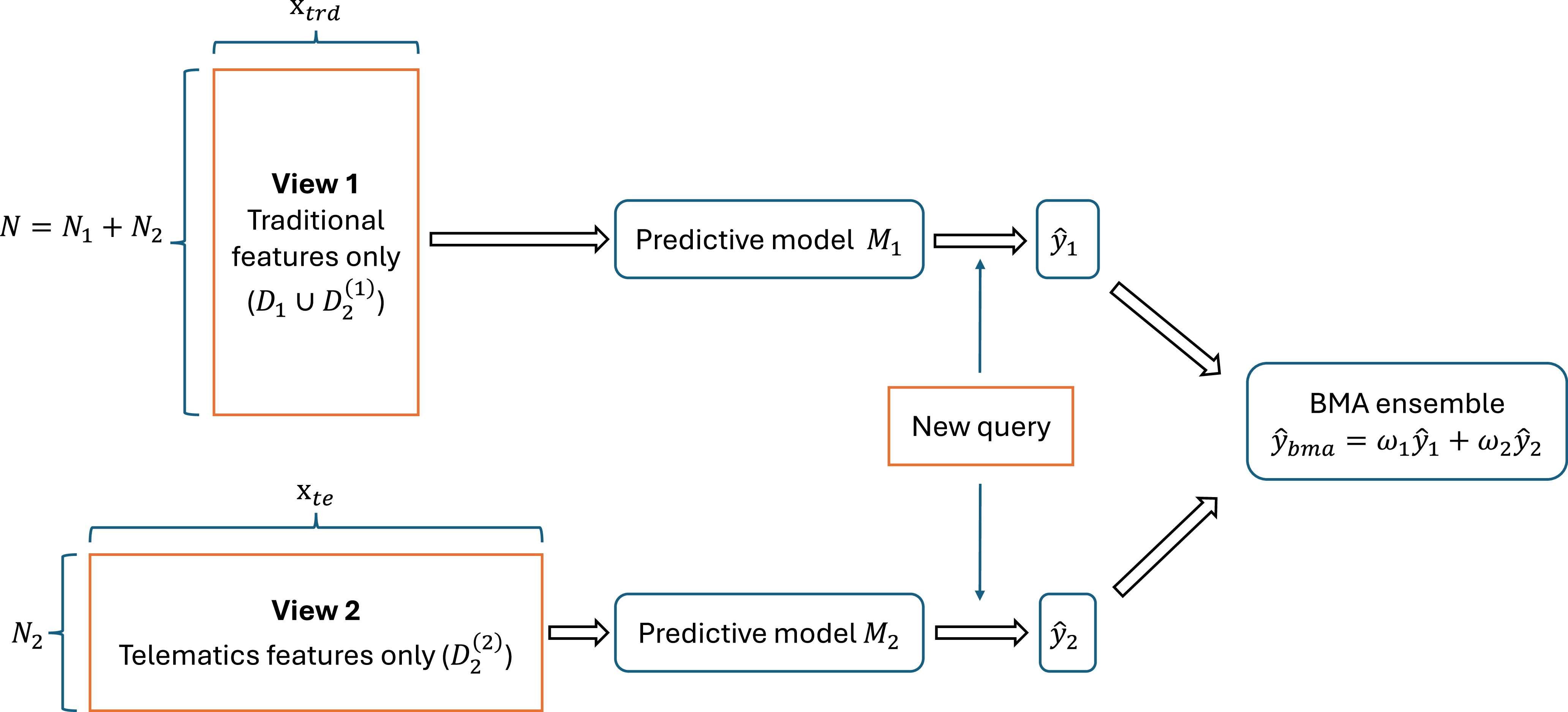
Figure 2 illustrates a BMA ensemble constructed from two individual models (
 $K=2$
), each trained from a different data view. Model
 $M_1$
is fitted using the traditional feature view, which is available for a large set of observations of size
 $N=N_1+N_2$
. In contrast, model
 $M_2$
is fitted using only the telematics feature view, which is available for the smaller subset of observations of size
 $N_2$
. For a new query, the traditional features
 $\mathbf{x}_{{trd}}$
are used to obtain the prediction
 $\widehat{y}_1$
from
 $M_1$
, while the telematics features
 $\mathbf{x}_{{te}}$
are used to obtain the prediction
 $\widehat{y}_2$
from
 $M_2$
. The two predictions are then combined through the BMA ensemble where the weights quantify the relative predictive effectiveness of the traditional and telematics views.
Example of the BMA ensemble with two individual models.

The weights (i.e., the posterior probabilities) play a key role in the BMA ensemble, and their values are estimated based on
 $\widehat{y}_j$
’s predictive performance on the validation data, denoted as
 $D_v$
.Footnote
1
Specifically, suppose that we have the prediction result
 $\widehat{y}_{ij}$
from model
 $M_j$
(
 $j=1,\ldots,K$
) for the
 $i{\rm th}$
policyholder in
 $D_{v}$
. The weights are then estimated by maximum likelihood from data
 $D_{v}$
. The log-likelihood function for the BMA model in Equation (1) is
 \begin{align*}\ell(w) = \sum_{i \in D_v} {\log \left(p_w(y_i \mid \widehat{y}_{i1},\ldots,\widehat{y}_{iK})\right)} =\sum_{i \in D_v} {\log \left(\sum_{j=1}^{K} w_j\, f_j(y_{i}\mid \widehat{y}_{ij})\right)}.\end{align*}
The maximum likelihood estimators of the weights may be obtained by the Expectation-Maximization (EM) algorithm (Dempster et al., Reference Dempster, Laird and Rubin1977; McLachlan and Krishnan, Reference McLachlan and Krishnan2007). Let
 $z_{ij}$
be the unobserved quantity, where
 $z_{ij} = 1$
if
 $\widehat{y}_j$
is the best prediction for policyholder i in
 $D_{v}$
, and
 $z_{ij} = 0$
otherwise. The EM algorithm iteratively alternates the expectation (E) step and the maximization (M) step. Starting with some initial values
 $w^{(0)}_j$
, the E step of the
 $l^{th}$
iteration estimates the
 $z_{ij}$
values as:
 \begin{align*}z^{(l)}_{ij} = \dfrac{w^{(l-1)}_{j} f_j(y_i\mid \widehat{y}_{ij})}{\sum_{q=1}^{K} w^{(l-1)}_{q} f_q(y_{i}\mid \widehat{y}_{iq})}. \end{align*}
In the M step, we update the weights by
 \begin{align*}w^{(l)}_{j} = \dfrac{1}{|D_v|}{\sum_{i \in D_v} z^{(l)}_{ij}}. \end{align*}
The E and M steps are iterated until convergence, for example, until the changes in the weights are no greater than a small tolerance.
Remark 1. This approach can also be used when the conditional density
 $f_j(y_i \mid \widehat{y}_{ij})$
also involves an additional distributional parameter, such as a dispersion or scale parameter. For example, one may write the component density as
 $f_j(y_i \mid \widehat{y}_{ij}, \phi)$
, where
 $\widehat{y}_{ij}$
determines the location or mean structure and
 $\phi$
controls the dispersion of the predictive distribution. The BMA likelihood can then be written as:
 \begin{align*}\ell(w,\phi)=\sum_{i\in D_v}\log\left\{\sum_{j=1}^Kw_j f_j(y_i \mid \widehat{y}_{ij},\phi)\right\}. \end{align*}
The EM algorithm can be extended directly to this setting. In the Estep, the posterior membership probabilities are computed using the current values of both the weights and the additional distributional parameter. In the Mstep, the weights are updated as before by averaging the posterior membership probabilities, while
 $\phi$
is updated by maximizing the corresponding weighted log-likelihood. Since the individual predictions
 $\widehat{y}_{ij}$
are treated as fixed inputs from the fitted candidate models, this maximization can be carried out using a standard numerical optimization routine over positive values of
 $\phi$
, for example, by a bounded positive interval.
The variance of
 $\widehat{Y}$
can be described as:
 \begin{align*} \mathrm{Var}(\widehat{Y}) = \sum_{j=1}^K w_j^2 \,\mathrm{Var}(\widehat{Y}_j) + 2 \sum_{1 \le j \lt k \le K} w_j w_k \,\mathrm{Cov}(\widehat{Y}_j, \widehat{Y}_k). \end{align*}
The first term aggregates the component variances, while the second term captures the interaction among models through their covariances. Assuming nonnegative correlations between individual model predictions, BMA prediction is more stable when the individual models are less correlated. In other words, the BMA ensemble is more effective when the constituent models, trained on potentially different data sources, offer diverse informational views.
Note that the model structure of BMA is superficially analogous to that of mixture models. However, BMA and mixture models are fundamentally different in both interpretation and estimation. A mixture model assumes that each data point is generated from one of the component distributions, and its weights characterize the latent data-generating mechanism. For a new observation, a mixture model outputs the posterior component probabilities (soft cluster assignments) that quantify the likelihood of membership in each component. In contrast, BMA focuses on combining predictions from multiple candidate models. When the analyst is uncertain which model is the “best”, BMA accounts for this model uncertainty through a weighted average of the individual model predictions. The weights in BMA reflect the relative plausibility of the models, not the probability that an observation belongs to a latent group.
The parameter estimation processes also differ significantly. In a mixture of Poisson models, the rate parameters are estimated jointly using the EM algorithm applied to all data because the latent component memberships must be inferred. In contrast, in the BMA ensemble, the predicted rates are obtained directly from the individual predictive models. BMA then treats these predicted rates as the component-specific parameters and combines them through a weighted average. Thus, BMA does not always require joint estimation of rate parameters or latent memberships as mixture models do.
It is worth noting that our application of the BMA method for multi-view ensemble learning deviates from conventional uses. Typically, BMA is employed to combine various predictive models that have been trained on the same dataset. Examples of such applications include weather forecasting (Raftery et al., Reference Raftery, Gneiting, Balabdaoui and Polakowski2005), debris-flow prediction (Tian et al., Reference Tian, Fan, Xiong and Li2023), and crop management (Fei et al., Reference Fei, Chen, Li, Ma and Xiao2023). In our approach, however, we modify the training data for each model, enabling each to generate predictions based on a single view. As illustrated in Figure 2, one model might be trained on a large dataset using only traditional features, while another is trained on a smaller dataset that includes additional telematics features. The BMA ensemble then integrates these single-view predictions to produce a comprehensive, multi-view forecast.
3.2. Selection of individual model components
The effectiveness of the BMA ensemble depends not only on the weight estimation procedure but also on the selection of the individual model components. Although the BMA framework can in principle accommodate a large number of candidate models, the inclusion of additional models should be guided by the objective of the analysis. The component models may represent different informational views arising from the unique data structure, where telematics information is available only for a subset of policyholders. Therefore, the construction of the candidate model set is an important modeling decision.
In general, the individual models may be selected to achieve two related but distinct objectives. The first objective is interpretability and transparency. In this case, the component models are designed to represent clearly distinguishable sources of information so that the BMA weights can be interpreted as the relative contribution of each information source. The second objective is predictive performance. In this case, the component models may be selected to increase predictive accuracy by combining models that capture different risk patterns. These two objectives are discussed below.
3.2.1. Model selection for interpretability and transparency
In terms of interpretability, it is desirable to use a small number of structurally distinct models. This allows the final BMA prediction to be expressed as a transparent combination of different risk perspectives. Suppose that two individual models are considered, where
 $M_1$
is trained using traditional rating variables only and
 $M_2$
is trained using telematics variables only. The BMA prediction then takes the form:
 \begin{align*}\widehat{y}_i=\widehat{w}_1\ \widehat{y}_{i1}+\widehat{w}_2 \ \widehat{y}_{i2}, \\[-10pt] \end{align*}
where
 $\widehat{y}_{i1}$
is the prediction from the traditional-feature model and
 $\widehat{y}_{i2}$
is the prediction from the telematics-feature model.
This structure provides a simple interpretation. The first component represents the risk assessment based on conventional actuarial information, while the second component represents the risk assessment based on observed driving behavior. Therefore, the final prediction is not produced by a single black-box model that internally mixes all variables. Instead, it is obtained as an explicit weighted combination of two distinct predictive views. The weight
 $\widehat{w}_1$
measures the degree to which the final prediction relies on traditional rating information, while
 $\widehat{w}_2$
measures the degree to which it relies on telematics information.
This type of structure can be extended to more than two components if the additional models represent meaningful and distinct risk perspectives. Another example may consider:
-
• Model 1: traditional rating variables;
-
• Model 2: driving intensity variables, such as mileage and trip frequency;
-
• Model 3: driving behavior variables, such as braking, acceleration, and speed patterns.
In this case, the BMA weights summarize the relative contribution of traditional risk information, exposure-related telematics information, and behavioral telematics information. Such a decomposition can be valuable when the goal is to understand which type of information contributes most to the final insurance risk prediction.
3.2.2. Model selection for predictive performance
Considering predictive performance, the individual model components may be selected more flexibly. In this case, the purpose of including multiple models is to improve the final prediction by combining models that make different types of errors or capture different aspects of the data. Since the BMA prediction is a weighted average of the individual predictions, the ensemble is most effective when the component models are both individually useful and sufficiently diverse. The BMA framework assigns larger weights to the models that provide stronger validation performance while assigning smaller weights to less useful models. In this way, the ensemble can benefit from both the stability of models trained on the larger traditional dataset and the additional behavioral information contained in the telematics variables.
In practice, a model that performs well but is nearly identical to an already included model may contribute little additional value, while a moderately performing model that captures a distinct information source may improve the ensemble. A practical selection rule is therefore to include a new model
 $M_{K+1}$
if it satisfies at least one of the following conditions: (i) it uses a distinct source or view of information; (ii) it provides improved validation performance; and (iii) it produces predictions that are not highly redundant with existing components. This rule prevents the BMA ensemble from becoming unnecessarily large while still allowing useful predictive information to be incorporated.
3.3. Consistency of BMA weights
For a weight vector
 \begin{align*} w = (w_1,\dots,w_K) \in \Delta_K \,:\!= \, \Big\{ w \in \mathbb{R}^K \,:\, w_j \ge 0,\ \sum_{j=1}^K w_j = 1 \Big\}, \end{align*}
let
 $\ell_n(w)$
be the BMA log-likelihood based on the validation data of size n,
 \begin{align*} \ell_n(w) = \sum_{i=1}^n \log\left( \sum_{j=1}^K w_j\, f_j(y_i \mid \widehat y_{ij}) \right), \end{align*}
and
 $\widehat{w}_n $
be the maximum likelihood estimator,
 \begin{align*} \widehat{w}_n = \arg\max_{w \in \Delta_K} \ell_n(w). \end{align*}
Let
 $E_T[\! \cdot \!]$
denote expectation under the true distribution of the data. We define the log-loss risk
 \begin{align*} R(w) \,:\!= \, E_T[ -\log p_w({Y}\mid \widehat y_1,\dots,\widehat y_K) ]. \end{align*}
and we are interested in the optimal weight vector that minimizes R(w). For BMA consistency, we assume the following assumptions:
-
(A1) (I.I.D. observations) Each data point
 $(y, \widehat{y}_1,\ldots,\widehat{y}_K)$
are i.i.d.
-
(A2) (Integrability) For every
$w \in \Delta_K$
,
\begin{align*} E_T[ | \log p_w({Y} \mid \widehat{y}_1,\ldots,\widehat{y}_K) | ] \lt \infty. \end{align*}
-
(A3) (Continuity and dominated convergence) For each
$(y,\widehat{y}_1,\ldots,\widehat{y}_K)$
, the map
$w \mapsto \log p_w(y \mid \widehat{y}_1,\ldots,\widehat{y}_K)$
is continuous on
$\Delta_K$
, and there exists an integrable function
$g(y,\widehat{y}_1,\ldots,\widehat{y}_K)$
such that
\begin{align*} \bigl| \log p_w(y \mid \widehat{y}_1,\ldots,\widehat{y}_K) \bigr| \le g(y,\widehat{y}_1,\ldots,\widehat{y}_K) \quad \text{for all } w \in \Delta_K. \end{align*}
-
(A4) (Uniqueness of the population maximizer) The function
$R(w) = E[\!-\log p_w({Y} \mid \widehat{y}_1,\ldots,\widehat{y}_K)]$
has a unique minimizer
$w^\star$
in
$\Delta_K$
. -
(A5) (Existence of a sample maximizer) For each n, there exists at least one maximizer
$\widehat{w}_n = \arg\max_{w \in \Delta_K} \ell_n(w)$
.


Note that
 $\Delta_K$
is compact and convex. Assumptions (A2) and (A3) are the usual regularity conditions required to apply a uniform law of large numbers to the class
 $\{\log p_w : w \in \Delta_K\}$
. Assumption (A2) is automatically satisfied for standard predictive likelihoods such as Poisson, Gamma, or Normal, for which the log-density has finite moments under the data-generating distribution.
For (A3), continuity of
 $w \mapsto \log p_w(y \mid \widehat{y}_1,\dots,\widehat{y}_K)$
follows immediately from the linear mixture structure and a valid dominating function can be taken as:
 \begin{align*} g(y,\widehat{y}_1,\dots,\widehat{y}_K) = -\log\Big( \min_{1 \le j \le K} f_j(y \mid \widehat{y}_j) \Big), \end{align*}
which is integrable under the true distribution when each component density
 $f_j$
is well behaved.
Regarding (A4), when the predictive densities
 $f_j(\cdot \mid \widehat{y}_j)$
are not identical as functions, the log-loss risk R(w) is strictly convex over
 $\Delta_K$
and thus has a unique minimizer
 $w^\star$
. Finally, (A5) holds automatically in our setting because
 $\Delta_K$
is compact and
 $\ell_n(w)$
is continuous in w, so by Weierstrass’ theorem there exists at least one maximizer
 $\widehat{w}_n = \arg\max_{w \in \Delta_K} \ell_n(w)$
for each n. Under these regular conditions, we have the following theorem.
Theorem 1 (Consistency of BMA Weights). Under Assumptions, any maximizer
 $\widehat{w}_n \in \arg \max_{w \in \Delta_K} \ell_n(w)$
satisfies
 \begin{align*} \widehat{w}_n \to w^\star \quad \text{almost surely (a.s.) as } n \to \infty. \end{align*}
In addition, if the EM algorithm converges to a global maximizer of
 $\ell_n(w)$
, then the BMA weights are also consistent for
 $w^\star$
.
Proof. Define the empirical risk
 \begin{align*} R_n(w) \,:\!= \, -\frac{1}{n} \ell_n(w) = -\frac{1}{n}\sum_{i=1}^n \log p_w(y_i\mid \widehat y_{i1},\dots,\widehat y_{iK}). \end{align*}
By (A1) and (A2),
 $R_n(w)\to R(w)$
for each fixed w. By (A3) and compactness of
 $\Delta_K$
, the uniform law of large numbers gives
 \begin{align*} \sup_{w\in\Delta_K} |R_n(w) - R(w)| \to 0 \quad a.s. \end{align*}
By (A4), R(w) has a unique minimizer
 $w^\star$
, and by (A5),
 $\widehat{w}_n$
is a minimizer of
 $R_n$
. Then the argmax theorem implies
 \begin{align*} \widehat{w}_n \to w^\star \quad a.s. \end{align*}
Each individual model
 $M_j$
corresponds to the vertex
 $e_j$
, and
 $R(e_j) = E[\!-\log f_j({Y}\mid \widehat y_j)]$
. Therefore, we have
 \begin{align*} R(w^\star) \le R(e_j),\quad j=1,\dots,K, \\[-10pt] \end{align*}
so the optimal BMA mixture achieves log-loss risk no larger than any individual model.
Many loss functions used in generalized linear models, such as deviance, are affine transformations of negative log-likelihood. Therefore, the optimality of
 $p_{w^\star}$
under log-loss directly implies optimality under deviance as well.
Our consistency result for the BMA weights is a special case of general M-estimation theory and is closely related to recent work on mixture likelihoods and model averaging. For finite mixture models, Chen (Reference Chen2017) provides a modern and unified treatment of consistency of maximum likelihood estimators under general mixture structures. More broadly, recent work on model averaging and forecast combinations also establishes asymptotic advantages of averaging over single models in misspecified settings; see, e.g., Le and Clarke (Reference Le and Clarke2022).
Lastly, the BMA framework and the consistency result presented in this section are applicable to a broad range of response types. It can be used for both claim frequency and claim severity prediction, as demonstrated in our case study in Section 4. For instance, for claim frequency, the conditional density
 $f_j(y \mid \widehat{y}_j)$
may be specified as a Poisson distribution with rate parameter
 $\widehat{y}_j$
for
 $j = 1,\dots,K$
, where
 $\widehat{y}_j$
denotes the predicted mean from model
 $M_j$
. For claim severity, an Exponential distribution with mean
 $\widehat{y}_j$
can be used, or alternatively, a Gamma predictive density can also be used, with
 $\widehat{y}_j$
representing the predicted mean from model
 $M_j$
and an additional dispersion parameter controlling the variability around that mean (as discussed in Remark 1).
4. Experimental study
4.1. Data
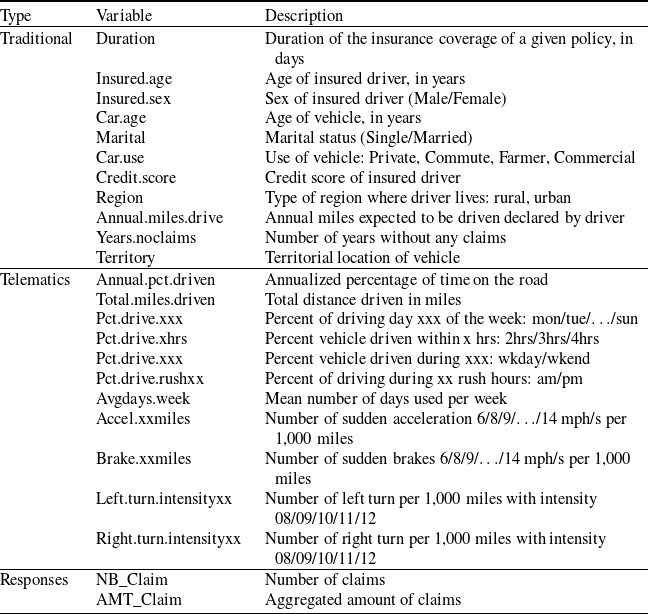
We evaluate the effectiveness of the proposed method using a synthetic dataset from So et al. (Reference So, Boucher and Valdez2021). Based on real-world data provided by a Canadian insurance company, the dataset was synthetically expanded using the Synthetic Minority Oversampling Technique (SMOTE) in combination with a feedforward Neural Network. It contains 100,000 policy records with 51 feature variables, grouped into two categories: traditional attributes (e.g., insured’s age and gender) and telematics-based measures (e.g., total distance driven, harsh accelerations, and harsh brakings). We consider two response variables: the number of observed claims and the average claim severity. A summary of the individual variables is provided in Table 1.
Description of individual variables in the synthetic telematics dataset.

Table 1. Long description
A table with two main categories of variables: Traditional and Telematics, each with specific descriptors. The Traditional category includes variables such as Duration, Insured.age, Insured.sex, Car.age, Marital, Car.use, Credit.score, Region, Annual.miles.drive, Years.noclaims, and Territory. The Telematics category includes variables like Annual.pct.driven, Total.miles.driven, Pct.drive.xxx, Pct.drive.xhrs, Pct.drive.xxx, Pct.drive.rushxx, Avgdays.week, Accel.xxmiles, Brake.xxmiles, Left.turn.intensityxx, and Right.turn.intensityxx. The Responses category includes NB_Claim and AMT_Claim. Each variable is described in terms of what it measures or represents.
4.2. Training individual models using random forest
For the individual predictive models, we employ random forest (RF); see, e.g., Breiman (Reference Breiman2001). RF is a well-established tree-based machine learning method, widely recognized for its strong predictive performance across diverse applications. As a nonparametric approach, RF can capture complex nonlinear relationships without relying on a predetermined functional form. Incorporating RF into the BMA ensemble leverages this modeling flexibility within a parametric aggregation framework, enabling downstream statistical inference when needed. Another important advantage of RF is the availability of out-of-bag (OOB) predictions, which help mitigate overfitting that can arise when the same dataset is used both to train individual models and to fit the BMA weights. In each bootstrap sample used to grow a tree, a subset of observations is left out and not used for fitting that tree. For each observation, the RF prediction can therefore be obtained by averaging only over the trees for which that observation was out-of-bag. These OOB predictions provide validation-type predictions because they are computed from trees that did not use the corresponding observation in model fitting. In our implementation, the BMA weights are estimated using these OOB predictions so that the validation likelihood is evaluated using predictions that are less directly affected by in-sample overfitting. Details on the use of OOB predictions in this context can be found in Gweon et al. (Reference Gweon, Li and Mamon2020). In addition, RF handles large sets of telematics features effectively, whereas classical generalized linear models may struggle with such high-dimensional inputs.
In this study, we consider three individual models. The first model,
 $M_1$
, is trained using all
 $N = N_1 + N_2$
policyholders in
 $D_1 \cup D^{(1)}_2$
, relying solely on traditional features (
 $\mathbf{x}_{{trd}}$
). We refer to
 $M_1$
as the traditional model. The second model,
 $M_2$
, is trained on policyholders in
 $D_2$
using telematics features only (
 $\mathbf{x}_{{te}}$
). Compared with
 $M_1$
,
 $M_2$
is fitted on a smaller dataset but uses individualized behavioral information derived from telematics data. We refer to
 $M_2$
as the naive model. Inspired by Ayuso et al. (Reference Ayuso, Guillen and Nielsen2019), we also construct a third model,
 $M_3$
, which refines the predictions of
 $M_1$
by incorporating telematics information. Specifically,
 $M_1$
is first used to generate initial predictions for policyholders in
 $D_2$
, and
 $M_3$
is then trained on
 $D^{(2)}_2$
using telematics features together with these predicted outcomes from
 $M_1$
. We refer to
 $M_3$
as the correction model.
Using these component models, we consider two BMA ensembles corresponding to the two modeling objectives discussed in Section 3.2. The first ensemble combines
 $M_1$
and
 $M_2$
and is used mainly for interpretability. As described in Section 3.2.1, its weights directly summarize the relative contribution of the traditional and telematics views. The second ensemble combines
 $M_1$
,
 $M_2$
, and
 $M_3$
and is used mainly for predictive performance. As described in Section 3.2.2, it allows the correction model to be included as an additional component when it provides useful and nonredundant predictive information.
4.3. Evaluation measures
Suppose that the test data contains n records. To assess the predictive performance, we use prediction mean squared error (MSE), the Poisson deviance statistic (
 $\text{DEV}_p$
) and the Gamma deviance statistic (
 $\text{DEV}_g$
) defined as:
 \begin{align*}\begin{aligned}\text{MSE} & = {\frac{1}{n} \sum_{i=1}^{n} \left( y_i - \widehat{y}_i\right)^2}, \end{aligned} \end{align*}
 \begin{align*}\begin{aligned} \text{DEV}_p &= \frac{2}{n} \sum_{i=1}^{n} \left( y_i \log\left(y_i / \widehat{y}_i \right) - \left(y_i - \widehat{y}_i \right) \right)\!, \\[3pt]\text{DEV}_g &= \frac{2}{n}\sum_{i=1}^n \left(\frac{y_i}{\widehat{y}_i} - \log\left(\frac{y_i}{\widehat{y}_i}\right) - 1 \right)\!.\end{aligned} \end{align*}
For all three metrics, lower values are favorable.
4.4. Case 1: Predicting the number of claims
From the original dataset, we randomly select
 $N_1$
= 20,000 records for
 $D_1$
. To account for potential selection biases in the telematics group, we consider three sampling schemes for generating the
 $D_2$
data. The age-based and favorable selection schemes, including the coefficient values in the sampling probabilities, were adopted from Peiris et al. (Reference Peiris, Jeong, Kim and Lee2024).
-
• Random selection: Records assigned to
$D_2$
are selected completely at random. -
• Age-based selection: Each record assigned to
$D_2$
is chosen with a sampling probability proportional to
$1/\{1+\exp(3x_{\text{Insured.age}})\}$
. This scheme reflects the assumption that younger policyholders are more likely to provide telematics information due to their greater openness to new technologies. -
• Favorable selection: Each record assigned to
$D_2$
is chosen with a sampling probability proportional to
$1/\{1+\exp(2y)\}$
. This scheme reflects the assumption that policyholders exhibiting safer driving behaviors are more likely to agree to telematics data collection.


For prediction, our primary interest lies in policyholders with available telematics information, as models incorporating telematics features cannot be applied to policyholders without telematics records. For policyholders without telematics information, prediction is obtained only from the traditional model
 $M_1$
, which uses traditional rating variables available for all policyholders. Accordingly, the BMA ensemble involving
 $M_2$
or
 $M_3$
is intended for the telematics-available population. We therefore construct the test data to represent the same underlying population as
 $D_2$
. For each sampling scheme, we construct a dataset of size
 $N_2+N_{ts}$
according to the corresponding sampling probabilities, where
 $N_{ts}$
denotes the size of the test data. From this dataset, we randomly select
 $N_2$
observations to form
 $D_2$
and use the remaining
 $N_{ts}$
observations as the test data. We consider
 $N_2 = 4{,}000$
, 8,000, and 12,000 to represent varying levels of telematics data availability for model training and set
 $N_{ts}=20{,}000$
.
For the BMA ensemble on claim frequency, we assume that the conditional probability function
 $f_j(y \mid \widehat{y}_j)$
in (1) follows a Poisson distribution with rate parameter
 $\widehat{y}_j$
, the prediction produced by model
 $M_j$
, that is,
 $f_j(y \mid \widehat{y}_j)=\dfrac{(\widehat{y}_j)^y e^{-\widehat{y}_j}}{y!}$
.
4.4.1. Interpreting the BMA model with
$M_1$
and
$M_2$


We first examine the BMA ensemble constructed using only
 $M_1$
and
 $M_2$
. This two-model BMA is useful for interpreting the relative contribution of the traditional and telematics-based predictive views. Recall that
 $M_1$
is trained on
 $D_1 \cup D_2^{(1)}$
using only traditional rating variables, whereas
 $M_2$
is trained on
 $D_2^{(2)}$
using telematics information. Therefore, the estimated BMA weights indicate how much the final prediction relies on the broad traditional risk information captured by
 $M_1$
and the telematics-based risk information captured by
 $M_2$
.
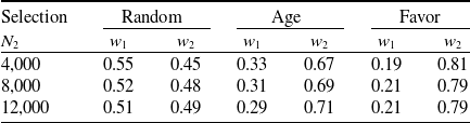
Table 2 reports the estimated BMA weights for
 $M_1$
and
 $M_2$
across the three selection scenarios. Under random selection, the two models receive similar weights. When
 $N_2=4{,}000$
, the traditional model receives a slightly larger weight (
 $w_1=0.55$
), reflecting the advantage of being trained on a larger dataset. As
 $N_2$
increases, however, the weight assigned to
 $M_2$
increases, and the two models receive nearly equal weights when
 $N_2=12{,}000$
. This suggests that when the telematics sample is drawn from the same population as the traditional sample, both traditional and telematics-based views contribute meaningfully to the final prediction.
Model weights.

Table 2. Long description
A table titled ‘Model weights’ with three columns labeled ‘Random’, ‘Age’, and ‘Favor’, and three rows labeled with selection sizes 4,000, 8,000, and 12,000. Each column contains two sub-columns labeled ‘w1’ and ‘w2’. Row 1: Random w1, 0.55; Random w2, 0.45; Age w1, 0.33; Age w2, 0.67; Favor w1, 0.19; Favor w2, 0.81. Row 2: Random w1, 0.52; Random w2, 0.48; Age w1, 0.31; Age w2, 0.69; Favor w1, 0.21; Favor w2, 0.79. Row 3: Random w1, 0.51; Random w2, 0.49; Age w1, 0.29; Age w2, 0.71; Favor w1, 0.21; Favor w2, 0.79.
A different pattern is observed under the age-based and favorable selection scenarios. In these cases, the BMA ensemble assigns substantially larger weights to
 $M_2$
than to
 $M_1$
. For the age-based selection scenario, the weight of
 $M_2$
ranges from 0.67 to 0.71, while for the favorable selection scenario it is approximately 0.79–0.81. These results indicate that when the telematics group differs systematically from the broader population, the model trained directly on the telematics group becomes more relevant for predicting policyholders with telematics information. In particular, under favorable selection, where safer drivers are more likely to appear in
 $D_2$
, the traditional model trained on the broader population receives relatively small weights. Thus, the BMA weights provide not only a measure of the relative predictive contribution of traditional and telematics information but also a diagnostic indication of population heterogeneity between
 $D_1$
and
 $D_2$
.
Figure 3 provides additional insight by showing the relationship between the predictions from
 $M_1$
and
 $M_2$
. Across all scenarios, the correlations between
 $\widehat{y}_{i1}$
and
 $\widehat{y}_{i2}$
are relatively low, indicating that the two models are not redundant. The correlations are particularly low under favorable selection, suggesting that the telematics-based view becomes most distinct when the telematics group is strongly selected.
Scatterplot of
 $M_1$
and
 $M_2$
predictions with correlations.

The correlations between
 $M_1$
and
 $M_2$
also tend to increase as
 $N_2$
becomes larger. This pattern should be interpreted as an empirical observation, since the two models are based on different feature views. One plausible explanation is that increasing
 $N_2$
improves both component models. Because
 $M_1$
is trained on
 $D_1 \cup D_2^{(1)}$
, its training size increases from
 $N_1+4{,}000$
to
 $N_1+12{,}000$
as
 $N_2$
grows. Similarly,
 $M_2$
is trained on a larger telematics sample. As a result, both models may produce more stable predictions and become better aligned with the same underlying claim-risk structure in the test population. As the common risk signal becomes more dominant relative to model estimation noise, the empirical correlation between
 $\widehat{y}_{i1}$
and
 $\widehat{y}_{i2}$
may increase.
Overall, the two-model BMA provides an interpretable decomposition of the final prediction. The traditional model
 $M_1$
contributes stable information from the larger dataset, while the telematics model
 $M_2$
contributes information that is more specific to policyholders with telematics records. The estimated weights show that the importance of these two views depends strongly on both the sampling mechanism and the size of the telematics dataset. Thus, even before considering additional model components, the BMA framework offers a transparent way to combine traditional and telematics-based risk assessments.
4.4.2. Improving predictive performance through BMA
We next consider the full BMA ensemble using
 $M_1$
,
 $M_2$
, and
 $M_3$
. While the two-model BMA in the previous subsection is used mainly to interpret the relative contribution of traditional and telematics-based views, the three-model ensemble is designed to improve predictive performance by adding the correction model
 $M_3$
. The correction model incorporates the prediction from
 $M_1$
together with telematics variables, allowing the telematics-based model to adjust the baseline risk information learned from the larger traditional-feature dataset.
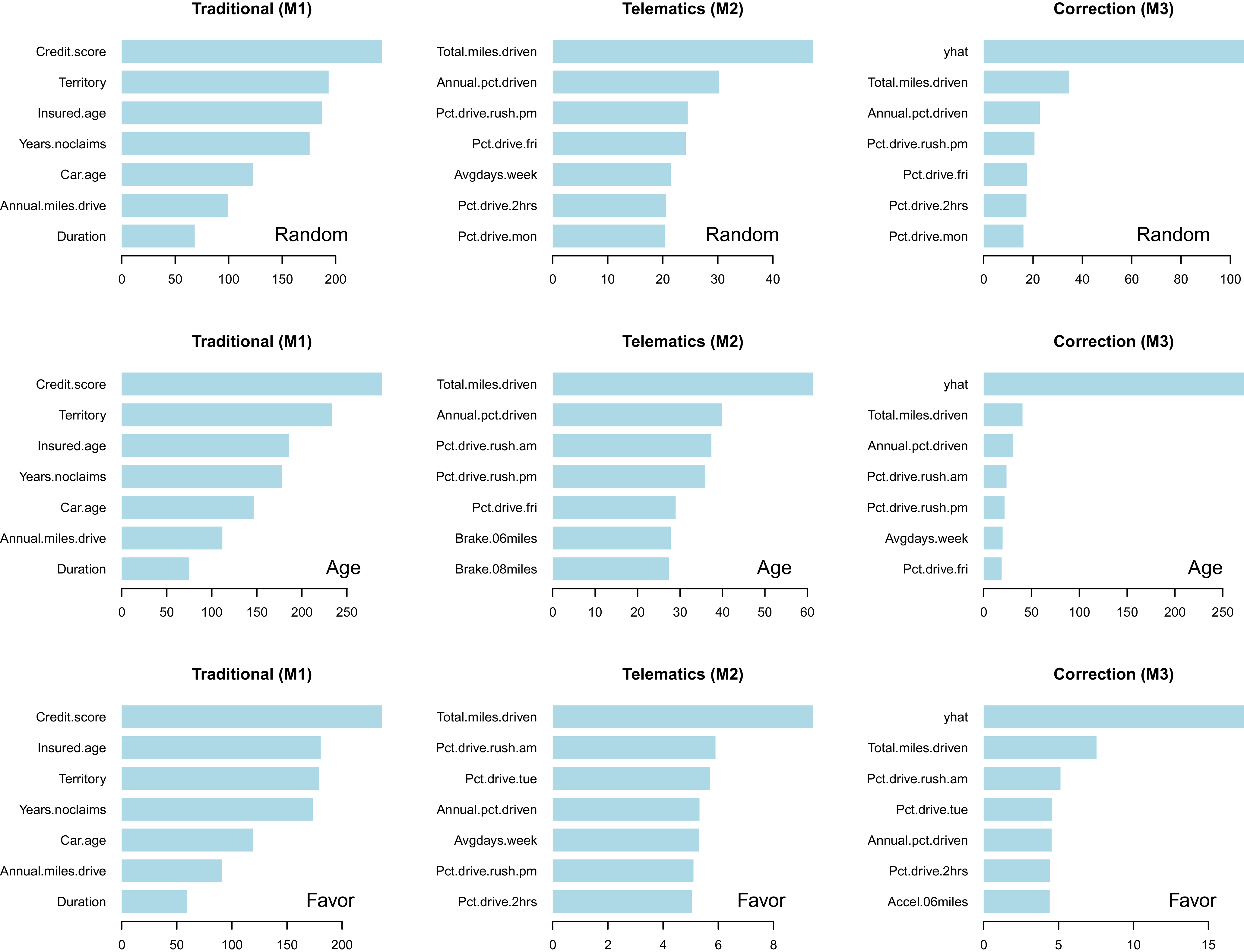
Before examining the BMA weights and prediction accuracy, we first inspect the variable importance plots of the individual RF models. Figure 4 presents the variable importance plots for
 $M_1$
,
 $M_2$
, and
 $M_3$
. For the traditional model
 $M_1$
, the most important features are credit score, territory, and the policyholder’s age, followed by years with no claims, car age, annual miles driven, and policy duration. These variables are conventional rating factors commonly used in auto insurance risk classification. In contrast, the naive telematics model
 $M_2$
is fitted using only telematics variables, without traditional rating variables. Its leading predictors include total miles driven, annual percentage driven, and rush-hour driving measures, suggesting that telematics information alone contains useful predictive information for claim frequency. For the correction model
 $M_3$
, the prediction from the traditional model, denoted by yhat, is by far the most important variable, while telematics variables such as total miles driven, annual percentage driven, and rush-hour driving measures provide additional explanatory information. This pattern indicates that
 $M_3$
uses yhat to retain the baseline risk information captured by the traditional rating variables and then uses telematics variables to refine or correct that baseline prediction.
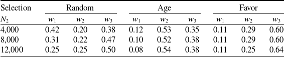
Table 3 reports the estimated BMA weights for the three-model ensemble. The weights reflect the relative predictive performance of
 $M_1$
,
 $M_2$
, and
 $M_3$
on the validation data. Under random selection, where
 $D_1$
and
 $D_2$
are drawn from the same population,
 $M_3$
receives relatively large weights, especially when
 $N_2 \geq 8{,}000$
. Under age-based selection, the BMA ensemble assigns the largest weights to
 $M_2$
. This indicates that when the telematics sample differs from the broader traditional sample in terms of age distribution, the model trained directly on the telematics group could better represent the target population than the correction model. Thus, the correction strategy is useful but not uniformly dominant; its effectiveness depends on the type of heterogeneity between
 $D_1$
and
 $D_2$
. Under favorable selection,
 $M_3$
receives the highest weights, followed by
 $M_2$
and then
 $M_1$
. This suggests that in this scenario, the correction model successfully combines the baseline risk information from
 $M_1$
with the telematics information available in
 $D_2$
. The relatively small weights assigned to
 $M_1$
are also consistent with the two-model BMA results in the previous subsection, where the traditional model became less relevant when the telematics group was strongly selected.
Model weights for the three-model BMA ensemble.

Table 3. Long description
A table comparing model weights for different selection methods. The table has three columns labeled Random, Age, and Favor, and three rows labeled with selection sizes 4,000, 8,000, and 12,000. Each cell contains a value representing the model weight for that selection method and size. For Random selection, the weights are 0.42, 0.20, 0.38 for 4,000; 0.31, 0.22, 0.47 for 8,000; and 0.25, 0.25, 0.50 for 12,000. For Age selection, the weights are 0.12, 0.53, 0.35 for 4,000; 0.10, 0.52, 0.38 for 8,000; and 0.08, 0.54, 0.38 for 12,000. For Favor selection, the weights are 0.11, 0.29, 0.60 for 4,000 and 8,000; and 0.11, 0.25, 0.64 for 12,000.
The variable importance plots for the individual models.

These results also illustrate how the BMA weights can be used to assess the completeness of a given integration strategy. If
 $M_3$
fully captured all useful information from both the traditional and telematics views, one would expect the BMA ensemble to place nearly all weight on
 $M_3$
. Instead, the weights remain distributed across
 $M_1$
,
 $M_2$
, and
 $M_3$
, and the dominant model changes across selection scenarios. This suggests that the correction approach is valuable, but that the traditional-only and telematics-only models still contribute additional predictive information beyond what is captured by the correction model alone. Thus, the BMA weights provide an empirical diagnostic of whether a proposed integration model fully reconciles the available views.
To further examine the dependence among the individual model predictions, Figure 5 presents pairwise scatterplots of
 $M_1$
,
 $M_2$
, and
 $M_3$
. The plots show that the association between
 $M_1$
and
 $M_2$
is weaker than the associations involving
 $M_3$
. This is expected because
 $M_3$
is constructed using the prediction from
 $M_1$
together with telematics variables. The relatively stronger association between
 $M_2$
and
 $M_3$
suggests that, although yhat is the most important individual feature in
 $M_3$
, the telematics variables still have substantial influence on the overall predictive behavior of the correction model.
Pairwise scatterplots of predictions from
 $M_1$
,
 $M_2$
, and
 $M_3$
across the three selection scenarios for
 $N_2=12{,}000$
.

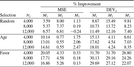
Table 4 summarizes the relative performance gains of the BMA method over the individual models. In terms of MSE, the BMA ensemble performs comparably to the best individual model in most scenarios. For example,
 $M_3$
is highly competitive under the random- and favorable selection scenarios, while
 $M_2$
performs well under age-based selection. The BMA ensemble adapts to these differences by assigning larger weights to the models that perform better on the validation data. In terms of Poisson deviance, the BMA method consistently outperforms all individual models across all selection scenarios. The gains are particularly large under favorable selection, where the improvement reaches approximately 20%–30%. These results are consistent with the theoretical property of BMA under log-loss-based criteria: by combining predictive distributions rather than selecting a single model, the BMA ensemble can achieve more robust predictive performance than any individual component model.
Relative performance gain of the BMA method over individual models in predicting claim counts.

Table 4. Long description
A table comparing the relative performance gain of the BMA method over individual models in predicting claim counts. The table has 3 groups of rows labeled Random, Age, and Favor, each with 3 rows for different values of N2: 4,000, 8,000, and 12,000. The columns are labeled MSE and DEV_p, with sub-columns M1, M2, and M3 under each. Row 1: Random, N2 4,000, MSE M1 3.59, MSE M2 8.00, MSE M3 1.13, DEV_p M1 8.67, DEV_p M2 15.49, DEV_p M3 9.81. Row 2: Random, N2 8,000, MSE M1 5.37, MSE M2 7.37, MSE M3 0.19, DEV_p M1 10.73, DEV_p M2 13.72, DEV_p M3 8.23. Row 3: Random, N2 12,000, MSE M1 6.57, MSE M2 6.81, MSE M3 0.24, DEV_p M1 11.49, DEV_p M2 12.16, DEV_p M3 7.40. Row 4: Age, N2 4,000, MSE M1 10.14, MSE M2 0.77, MSE M3 1.75, DEV_p M1 15.13, DEV_p M2 4.11, DEV_p M3 6.61. Row 5: Age, N2 8,000, MSE M1 13.01, MSE M2 0.55, MSE M3 2.06, DEV_p M1 17.62, DEV_p M2 4.54, DEV_p M3 7.03. Row 6: Age, N2 12,000, MSE M1 14.61, MSE M2 0.55, MSE M3 2.47, DEV_p M1 18.01, DEV_p M2 4.24, DEV_p M3 8.35. Row 7: Favor, N2 4,000, MSE M1 20.05, MSE M2 4.33, MSE M3 0.33, DEV_p M1 31.70, DEV_p M2 31.70, DEV_p M3 26.80. Row 8: Favor, N2 8,000, MSE M1 17.71, MSE M2 4.58, MSE M3 0.18, DEV_p M1 30.13, DEV_p M2 29.16, DEV_p M3 24.26. Row 9: Favor, N2 12,000, MSE M1 16.86, MSE M2 5.26, MSE M3 0.13, DEV_p M1 29.69, DEV_p M2 27.12, DEV_p M3 22.07.
4.5. Case 2: Predicting the severity of claims
Beyond claim counts, we also evaluated the BMA framework for predicting claim severity. Among the 100,000 policy records, 3,864 had positive claim amounts. For the severity analysis, we used these 3,864 records as the full dataset. Given the smaller sample size, we fixed
 $N_1=1{,}000$
and considered
 $N_2=500$
and 1,000, with the remaining observations used as the test data. For the BMA ensemble in Case 2, we specify the conditional distribution
 $f_j(y \mid \widehat{y}_j)$
in (1) as a Gamma distribution for positive claim severity, that is,
 \begin{align*}f_j(y \mid \widehat{y}_j)=\frac{1}{\Gamma(1/\phi) (\phi \widehat{y}_j) ^{1/\phi}}y^{\frac{1}{\phi}-1} e^{-\frac{y}{\phi \widehat{y}_j}}. \end{align*}
Here,
 $\widehat{y}_j$
is the predicted mean claim severity produced by model
 $M_j$
, and the common dispersion parameter
 $\phi$
is shared across all component models.
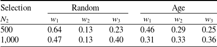
Table 5 reports the estimated BMA weights for claim severity. When
 $N_2=500$
, the traditional model
 $M_1$
receives relatively large weights, reflecting the limited amount of telematics data available for training the telematics-based models. As
 $N_2$
increases to 1,000, the weights assigned to the telematics-related models become more competitive. This pattern is consistent with the claim-frequency results in Case 1: as more telematics observations become available, models using telematics information become more stable and more influential in the BMA ensemble. However, the differences in weights are less pronounced than in Case 1, partly because the severity analysis uses a smaller dataset and the training sample sizes allocated to the component models are closer.
Model weights for the three-model BMA ensemble.

Table 5. Long description
A table comparing model weights for different selection criteria and sample sizes. The table has two rows and six columns. The columns are labeled ‘Selection’, ‘Random w1’, ‘Random w2’, ‘Random w3’, ‘Age w1’, ‘Age w2’, and ‘Age w3’. The row labels are ‘500’ and ‘1,000’. Row 1: Selection, 500; Random w1, 0.64; Random w2, 0.13; Random w3, 0.23; Age w1, 0.46; Age w2, 0.29; Age w3, 0.25. Row 2: Selection, 1,000; Random w1, 0.47; Random w2, 0.13; Random w3, 0.40; Age w1, 0.31; Age w2, 0.33; Age w3, 0.36.
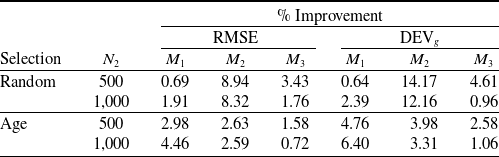
Table 6 summarizes the relative performance gains of the BMA method over the individual models. The best individual model varies across the selection scenarios and training sizes. For example,
 $M_1$
is highly competitive when telematics data are limited, while
 $M_2$
and
 $M_3$
become more competitive depending on the selection mechanism and the size of
 $D_2$
. Across all settings, the BMA ensemble delivers strong predictive performance and generally improves upon each individual model under both RMSE and Gamma deviance. These results suggest that the proposed BMA approach is not limited to claim-frequency prediction but can also provide robust predictive performance for claim severity.
5. Concluding remarks
This study proposed a multi-view BMA ensemble framework for auto insurance data with heterogeneous feature availability. In the data structure considered here, traditional rating variables are available for the full portfolio, whereas telematics variables are observed only for a smaller subset of policyholders. The proposed framework addresses this structure by training view-specific predictive models and combining their predictions through validation-based BMA weights. In particular, the traditional model captures broad risk information from conventional rating variables, while the telematics model captures driving behavior information from the UBI subset.
Relative performance gain of the BMA method over individual models in predicting claim severity.

Table 6. Long description
A table comparing the relative performance gains of the BMA method over individual models in predicting claim severity. The table has 6 rows and 8 columns. Column headers are Selection, N 2, % Improvement RMSE M 1, % Improvement RMSE M 2, % Improvement RMSE M 3, % Improvement DEV g M 1, % Improvement DEV g M 2, and % Improvement DEV g M 3. Row labels are Random 500, Random 1,000, Age 500, and Age 1,000. Row 1: Random, 500, 0.69, 8.94, 3.43, 0.64, 14.17, 4.61. Row 2: Random, 1,000, 1.91, 8.32, 1.76, 2.39, 12.16, 0.96. Row 3: Age, 500, 2.98, 2.63, 1.58, 4.76, 3.98, 2.58. Row 4: Age, 1,000, 4.46, 2.59, 0.72, 6.40, 3.31, 1.06.
The results show that the BMA framework provides both predictive and interpretive benefits. The estimated weights summarize the relative contribution of traditional and telematics-based risk assessments. Under random selection, the traditional and telematics views both contribute meaningfully to the final prediction. Under age-based and favorable selection, the BMA weights shift toward models trained directly on the telematics group, indicating that the telematics view becomes more relevant when the UBI subset differs from the broader portfolio. Thus, the BMA weights provide a transparent diagnostic tool for understanding how different sources of information contribute to insurance risk prediction.
The proposed method also provides practical gains for risk assessment and management. By combining traditional and telematics-based predictions, the BMA ensemble can produce more reliable risk scores for policyholders with telematics records than relying on either source alone. This is useful for pricing and underwriting because it allows insurers to incorporate behavioral driving information without discarding the stability provided by the larger traditional dataset. The weighting mechanism also helps manage model uncertainty: when the best individual model changes across selection scenarios or training sizes, BMA adapts by assigning larger weights to the models with stronger validation performance. As a result, the method offers a more robust basis for portfolio segmentation, risk monitoring, and UBI program design.
In the claim-frequency analysis, the BMA ensemble performs comparably to the best individual model in terms of MSE and consistently improves Poisson deviance across all selection scenarios. The improvement is particularly large under favorable selection, where the telematics sample is most distinct from the broader population. In the claim severity analysis, the BMA ensemble also delivers strong predictive performance and generally improves upon the individual models under both MSE and Gamma deviance. These results suggest that the proposed framework is flexible enough to support both claim frequency and claim severity prediction.
Future work may extend the proposed framework in several directions. First, additional component models may be incorporated when they represent distinct and meaningful sources of risk information, such as separating telematics variables into driving exposure and driving behavior views. Second, alternative predictive distributions such as lognormal densities could also be considered. Finally, future research may investigate segment-specific or time-varying BMA weights to reflect changes in telematics adoption, portfolio composition, or driving behavior over time.
Acknowledgements
This research is supported by the Natural Sciences and Engineering Research Council of Canada (NSERC, grant numbers RGPIN-2026-07648 (PI: Shu Li) and RGPIN-2022-04698 (PI: Hyukjun Gweon)).

 M1
 M2

 M1
 M2
 M3
 N2=12,000

 Open access

