1. Introduction
The ability to predict morphodynamic changes in rivers, estuaries and coastal environments is of central importance for both fundamental research and engineering applications. Accurate models of sediment transport and bed evolution are required to design and maintain hydraulic structures, to assess flood risk, and to understand the long-term dynamics of natural systems.
The prevailing paradigm for simulating morphodynamics is based on the solution of a coupled set of partial differential equations (e.g. Siviglia et al. Reference Siviglia, Stecca, Vanzo, Zolezzi, Toro and Tubino2013; Villaret et al. Reference Villaret, Hervouet, Kopmann, Merkel and Davies2013; Vanzo et al. Reference Vanzo, Peter, Vonwiller, Bürgler, Weberndorfer, Siviglia, Conde and Vetsch2021). The hydrodynamics are typically described by the shallow-water equations, while the evolution of the bed is governed by mass conservation. These are complemented by closure relations for bed friction and sediment transport, which introduce empirical or semi-empirical representations of unresolved physical processes.
When the problem involves mixed-size sediment, the state-of-the-art approach to representing the evolution of sediment composition is the active-layer model (Hirano Reference Hirano1971). This framework has been successfully applied across a broad range of cases, from laboratory experiments to large-scale riverine and coastal systems (van der Wegen and Jaffe Reference van der Wegen and Jaffe2014; Viparelli et al. Reference Viparelli, Moreira and Blom2017; Colombini and Carbonari Reference Colombini and Carbonari2020). The active-layer model conceptualises the bed as comprising a layer of sediment (the active layer) that interacts with the overlying flow and the underlying substrate. The sediment transport composition depends on the composition of the active layer. The main assumption and key point in the active-layer model is that only two processes lead to a change in active-layer composition: (i) sediment transport gradients; and (ii) sediment exchange between the active layer and the substrate due to aggradation, degradation or a change in active-layer thickness. Hence, for instance, sediment sorting at the lee face of bedforms is neglected (Blom et al. Reference Blom, Ribberink and de Vriend2003; Blom and Parker Reference Blom and Parker2004; Blom et al. Reference Blom, Parker, Ribberink and de Vriend2006). Figure 1 presents a sketch of the active-layer model.
Model sketch: (a) real situation; (b) model schematisation. The bed elevation (
 $\eta$
) represents a mean over several bedforms unresolved by the flow equations. The flow is described by a water column (
 $h$
), and specific discharges in
 $x$
and
 $y$
directions (
 $q_{\textit{x}}$
and
 $q_{\textit{y}}$
). The bed is composed of mixed-size sediment with an active layer of thickness
 $L_{\textit{a}}$
. Variables
 $F_{\textit{a}k}$
and
 $f^{\textit{I}}_{k}$
are the volume fraction content of size fraction
 $k$
in the active layer, and at the interface between the active layer and the substrate, respectively. A flux of sediment may exist between the substrate and the active layer. Under aggradational conditions, sediment from the active layer is transferred to the substrate and vice versa under degradational conditions. The sediment transport rates of size fraction
 $k$
in
 $x$
and
 $y$
direction are
 $q_{\textit{bx}k}$
and
 $q_{\textit{by}k}$
, respectively.

The thickness of the active layer depends on the vertical mixing processes relevant in the time scale under consideration (Chavarrías et al. Reference Chavarrías, Ottevanger, Sloff and Mosselman2022). Over short time scales, the active layer is thin as only the uppermost sediment is mobilised by the flow. Over longer time scales, the active layer thickens as sediment mixing processes (e.g. due to bedform migration) affect deeper layers of the bed. The active-layer thickness is therefore a representation of the depth over which sediment mixing processes occur within the bed over the time scale of interest.
Despite its wide use and apparent robustness, the active-layer model exhibits a limitation that becomes manifest under certain conditions. In particular, it can render the governing system of equations ill-posed (Ribberink Reference Ribberink1987; Stecca et al. Reference Stecca, Siviglia and Blom2014; Chavarrías et al. Reference Chavarrías, Stecca and Blom2018, Reference Chavarrías, Schielen, Ottevanger and Blom2019a ).
An ill-posed formulation gives rise to unphysical grid-scale oscillations in the numerical solution (Kabanikhin Reference Kabanikhin2008). The underlying issue is that the governing equations lack a mechanism that suppresses arbitrarily short waves. In a physically consistent system, small-scale fluctuations are subject to a cutoff in the short-wave range, ensuring that ever shorter perturbations do not lead to unbounded growth rates (Joseph and Saut Reference Joseph and Saut1990). The emergence of ill-posedness is therefore not merely a numerical artefact, but rather a symptom that a key physical process is missing from the mathematical formulation (Fowler Reference Fowler1997).
Chavarrías et al. (Reference Chavarrías, Stecca, Siviglia and Blom2019b ) devised a regularisation strategy to guarantee that the one-dimensional active-layer model is unconditionally well-posed. The strategy can be classified as a preconditioning technique (Turkel Reference Turkel1999) and is based on modifying the time scale of mixing processes. Chavarrías et al. (Reference Chavarrías, Stecca, Siviglia and Blom2019b ) proved that, under conditions in which the active-layer model is ill-posed, the system is regularised by sufficiently slowing down the mixing processes. The physical interpretation of the strategy is that the active-layer model is ill-posed when it becomes incapable of capturing fast mixing processes occurring in nature. The slow down of the mixing processes implies an increase in the time scale under consideration. Worded differently, the time scale over which the model variables are representative of the conditions of the bed is increased.
Chavarrías et al. (Reference Chavarrías, Stecca, Siviglia and Blom2019b ) tested the results of the regularisation strategy against data from laboratory experiments and confirmed that the regularised active-layer model captures the behaviour of the system averaged over the passage of several bedforms causing fast mixing of sediment. In other words, the active-layer model is missing the physical process responsible for the fast mixing waves observed in their laboratory experiments. Yet, the strategy was devised for one-dimensional conditions. Here, we propose a regularisation strategy that guarantees that the two-dimensional active-layer model is well-posed.
The present work addresses the issue of ill-posedness by deriving a consistent two-dimensional extension of the active-layer framework, and demonstrating its implications through theoretical analysis and numerical experiments. In doing so, we provide a physically grounded remedy to the ill-posedness of mixed-sediment morphodynamic models, thereby advancing the reliability of predictive modelling in sediment-laden flows.
The document is organised as follows. In § 2, we introduce the system of equations modelling two-dimensional morphodynamic bed development with mixed-size sediment. In § 3, we propose two regularisation strategies. In § 4, we linearise the model to be able to conduct a perturbation analysis. Analytical results of the perturbation analysis are described in § 5. In § 6, we apply the successful regularisation strategy to an existing laboratory case study. Results are discussed in § 7, while § 8 reports the conclusions.
2. Governing equations
The vertical length and velocity scales of the flow are assumed to be negligible with respect to the horizontal ones. The ratio between the solid and liquid discharge is assumed small (below
 $6\times 10^{-3}$
(Garegnani et al. Reference Garegnani, Rosatti and Bonaventura2011, Reference Garegnani, Rosatti and Bonaventura2013)), such that the clear-water approximation is applicable. Under these conditions, the flow is described using the depth-averaged shallow water equations (e.g. Vreugdenhil Reference Vreugdenhil1994):
 \begin{align} \frac {\partial h}{\partial t}+\frac {\partial q_{\textit{x}}}{\partial x}+\frac {\partial q_{\textit{y}}}{\partial y}&=0 ,\end{align}
 \begin{align} \frac {\partial q_{\textit{x}}}{\partial t}+\frac {\partial (q_{\textit{x}}^2/h+gh^2/2)}{\partial x}+\frac {\partial \left (\dfrac {q_{\textit{x}}q_{\textit{y}}}{h}\right )}{\partial y}+gh\frac {\partial \eta }{\partial x} &= -gh S_{\textit{fx}} ,\end{align}
 \begin{align} \frac {\partial q_{\textit{y}}}{\partial t}+\frac {\partial (q_{\textit{y}}^2/h+gh^2/2)}{\partial y}+\frac {\partial \left (\dfrac {q_{\textit{x}}q_{\textit{y}}}{h}\right )}{\partial x}+gh\frac {\partial \eta }{\partial y} &= -gh S_{\textit{fy}} ,\end{align}
where
 $(x,y)$
 $[\textrm {m}]$
are Cartesian coordinates and
 $t$
 $[\textrm {s}]$
is the time coordinate. Variable
 $h$
 $[\textrm {m}]$
is the flow depth. Variables
 $(q_{\textit{x}},q_{\textit{y}})$
 $[\textrm{m}^{2}\,\textrm{s}^{-1}]$
are the specific water discharges in the
 $x$
and
 $y$
direction, respectively. Variable
 $\eta$
 $[\textrm {m}]$
is the bed elevation and
 $g$
 $[\textrm{m s}^{-2}]$
the acceleration due to gravity. The friction slopes
 $(S_{\textit{fx}},S_{\textit{fy}})$
[
 $-$
] are
 \begin{equation} S_{\textit{fx}}=\frac {C_{\textit{f}}q_{\textit{x}}Q}{gh^3} , \quad S_{\textit{fy}}=\frac {C_{\textit{f}}q_{\textit{y}}Q}{gh^3} , \end{equation}
where parameter
 $C_{\textit{f}}$
[
 $-$
] is a constant non-dimensional friction coefficient (Ikeda et al. Reference Ikeda, Parker and Sawai1981; Schielen et al. Reference Schielen, Doelman and de Swart1993; Chavarrías et al. Reference Chavarrías, Schielen, Ottevanger and Blom2019a
) and
 $Q$
 $[\textrm{m}^{2}\,\textrm{s}^{-1}]$
is the magnitude of the specific water discharge.
The additional terms originating from the difference between the velocity at a certain elevation in the water column and the depth-averaged velocity (i.e. secondary flow) are neglected, as they do not play a role in the well-posedness of the morphodynamic system of equations (Chavarrías et al. Reference Chavarrías, Schielen, Ottevanger and Blom2019a ). For the same reason, the streamwise normal Reynolds stress is neglected. In other words, no eddy viscosity is considered. This stress becomes particularly relevant under high-Froude conditions for properly capturing the behaviour of the flow modes and the formation of roll waves (Needham and Merkin Reference Needham and Merkin1984; Balmforth and Mandre Reference Balmforth and Mandre2004; Balmforth and Vakil Reference Balmforth and Vakil2012; Rodrigues and Zumbrun Reference Rodrigues and Zumbrun2016; Barker and Gray Reference Barker, Johnson, Noble, Rodrigues and Zumbrun2017; Barker et al. Reference Barker, Johnson, Noble, Rodrigues and Zumbrun2017). While viscosity matters for obtaining a well-posed model that includes secondary flow (Chavarrías et al. Reference Chavarrías, Schielen, Ottevanger and Blom2019a ), the active-layer model is ill-posed due to a lack of other physical mechanisms and viscosity does not play a significant role (further discussed in § 7).
The sediment forming the bed is assumed to be a mixture of an arbitrary number
 $N$
of non-cohesive sediment fractions with equal density characterised by a grain size
 $d_k$
 $[\textrm {m}]$
, where the subscript
 $k$
denotes the grain-size fraction in increasing order. Compaction is neglected such that porosity is constant. Sediment inertia is neglected such that the sediment transport rate reacts instantaneously to flow changes (i.e. the sediment transport rate is always at capacity). In this simplified case, bed elevation change is represented by the Exner (Reference Exner1920) equation (see e.g. Paola and Voller Reference Paola and Voller2005):
 \begin{equation} \frac {\partial \eta }{\partial t}+\frac {\partial q_{\textit{bx}}}{\partial x}+\frac {\partial q_{\textit{by}}}{\partial y}=0 , \end{equation}
where
 $q_{\textit{bx}}=\sum _{k=1}^{N}q_{\textit{bx}k}$
 $[\textrm{m}^{2}\,\textrm{s}^{-1}]$
and
 $q_{\textit{by}}=\sum _{k=1}^{N}q_{\textit{by}k}$
 $[\textrm{m}^{2}\,\textrm{s}^{-1}]$
are the total specific (i.e. per unit of differential length) sediment transport rates including pores in the
 $x$
and
 $y$
direction, respectively. The variables
 $q_{\textit{bx}k}$
 $[\textrm{m}^{2}\,\textrm{s}^{-1}]$
and
 $q_{\textit{by}k}$
 $[\textrm{m}^{2}\,\textrm{s}^{-1}]$
are the specific sediment transport rates of size fraction
 $k$
including pores.
The active-layer model (Hirano Reference Hirano1971) describes changes in bed composition. Mass conservation of sediment of size fraction
 $k$
in the active layer reads
 \begin{equation} \frac {\partial M_{\textit{a}k}}{\partial t}+f^{\textit{I}}_{k}\frac {\partial \left (\eta -L_{\textit{a}}\right )}{\partial t}+\frac {\partial q_{\textit{bx}k}}{\partial x}+\frac {\partial q_{\textit{by}k}}{\partial y}=0 \quad k\in \{1,N-1\} , \end{equation}
where
 $M_{\textit{a}k}=F_{\textit{a}k}L_{\textit{a}}$
 $[\textrm {m}]$
is the volume of sediment of size fraction
 $k$
per unit of bed area in the active layer. The variable
 $L_{\textit{a}}$
 $[\textrm {m}]$
is the active-layer thickness. The variable
 $F_{\textit{a}k}\in [0,1]$
is the volume fraction content of sediment of size fraction
 $k$
in the active layer. The variable
 $f^{\textit{I}}_{k}\in [0,1]$
is the volume fraction content of sediment of size fraction
 $k$
at the interface between the active layer and the substrate. The volume fraction contents are constrained by the conditions:
 \begin{equation} \sum _{k=1}^N F_{\textit{a}k}=1 , \quad \sum _{k=1}^N f_{k}^{\textit{I}}=1 . \end{equation}
An important feature is that sediment below the active layer may have a different composition than the one in the active layer. This is actually the most common case in rivers, as the bed surface is usually coarser than the substrate due to armouring processes (e.g. Parker and Sutherland Reference Parker and Sutherland1990). Hence, under degradational conditions, sediment from the substrate is transferred to the active layer and
 $f^{\textit{I}}_{k}\neq F_{\textit{a}k}$
. Under aggradational conditions, sediment in the active layer is transferred to the substrate and
 $f^{\textit{I}}_{k}=F_{\textit{a}k}$
.
The system is complete with
 $N-1$
conservation equations describing changes in substrate composition. These do not play a role in the analysis as they are linearly dependent on the active-layer equations (Stecca et al. Reference Stecca, Siviglia and Blom2014). The reader is referred to Chavarrías et al. (Reference Chavarrías, Stecca and Blom2018) and Chavarrías et al. (Reference Chavarrías, Schielen, Ottevanger and Blom2019a
) for insight into the role of the substrate.
A more accurate representation of the mixing processes may be obtained if the active-layer thickness varies in space and time according to the local properties of the bed and the flow. This approach implies that the active-layer thickness is a dependent variable of the system. Chavarrías et al. (Reference Chavarrías, Stecca and Blom2018) showed that when considering a variable active-layer thickness depending on the flow depth for considering dependence on dune height, the domain in which the active-layer model is ill-posed slightly increases. However, the main cause of ill-posedness (degradation into a finer substrate) is independent of considering a variable active-layer thickness (Chavarrías et al. Reference Chavarrías, Stecca and Blom2018). For this reason, a constant active-layer thickness
 $L_{\textit{a}}$
is assumed.
The sediment transport magnitude (
 $q_{\textit{b}k}$
) depends on the non-dimensional sediment transport rate (
 $q^*_{\textit{b}k}$
) following Einstein (Reference Einstein1950):
 \begin{equation} q_{\textit{b}k}=F_{\textit{a}k}Q_{\textit{b}k}=F_{\textit{a}k}\frac {\sqrt {g R d_k^3}}{\left (1-p\right )}q^*_{\textit{b}k} , \end{equation}
where
 $p$
is the porosity and
 $R=\rho _{\textit{s}}/\rho _{w}-1$
[
 $-$
] is the submerged sediment density in which
 $\rho _{\textit{s}}={2650}\,{\textrm{kg}\,\textrm{m}^{-3}}$
is the sediment density and
 $\rho _{w}={1000}\,{\textrm{kg}\,\textrm{m}^{-3}}$
is the water density. Variable
 $Q_{\textit{b}k}$
represents the sediment transport capacity (Deigaard and Fredsøe Reference Deigaard and Fredsøe1978; Ribberink Reference Ribberink1987; Armanini Reference Armanini1995). A myriad of sediment-transport relations exist that relate the Shields (Reference Shields1936) stress,
 \begin{equation} \theta _k=\frac {C_{\textit{f}}\left ({Q}/{h}\right )^2}{\textit{gRd}_k} , \end{equation}
to the non-dimensional sediment transport rate, such as those by Meyer-Peter and Müller (Reference Meyer-Peter and Müller1948), Engelund and Hansen (Reference Engelund and Hansen1967), Ashida and Michiue (Reference Ashida and Michiue1971) or Wilcock and Crowe (Reference Wilcock and Crowe2003). In some of these relations, a hiding-exposure relation models the fact that, in a mixed bed, sediment finer than the mean is less exposed to the flow (hides) than it would be under uniform sediment conditions, and vice versa for sediment coarser than the mean (Egiazaroff Reference Egiazaroff1965). Furthermore, the direction of the sediment transport is affected by the bed slope (van Bendegom Reference van Bendegom1947).
Appendix A contains details on the sediment transport closure relations. Here, we summarise the dependencies of the sediment transport on the dependent variables of the system (
 $h$
,
 $q_{\textit{x}}$
,
 $q_{\textit{y}}$
,
 $\eta$
,
 $M_{\textit{a}k}$
), as it is important to understand the terms appearing in the linear system.
The sediment transport depends on the magnitude of the sediment transport and its direction:
 \begin{equation} \left (q_{\textit{bx}k},q_{\textit{by}k}\right )=f\left (q_{\textit{b}k},\varphi _{\textit{s}k}\right) , \end{equation}
where
 $\varphi _{\textit{s}k}$
[
 $-$
] is the angle of the sediment transport vector, which depends on the flow direction, bed slope and Shields (Reference Shields1936) stress (Appendix A):
 \begin{equation} \varphi _{\textit{s}k}=f\left (q_{\textit{x}},q_{\textit{y}},\eta ,\theta _k\right ) . \end{equation}
The Shields (Reference Shields1936) stress depends on the flow variables as shown in (2.9):
 \begin{equation} \theta _k=f\left (q_{\textit{x}},q_{\textit{y}},h\right ) . \end{equation}
The magnitude of the sediment transport depends on the volume fraction content in the active layer (hence, on the volume of sediment in the active layer) and the non-dimensional sediment transport rate:
 \begin{equation} q_{\textit{b}k}=f\left (M_{\textit{a}k},q^*_{\textit{b}k}\right ) . \end{equation}
The non-dimensional sediment transport rate depends on the Shields (Reference Shields1936) stress and on the hiding-exposure effects (
 $\xi _k$
, Appendix A):
 \begin{equation} q^*_{\textit{b}k}=f\left (\theta _k,\xi _{k}\right ) . \end{equation}
The hiding-exposure effects depend on the grain size and the mean grain size:
 \begin{equation} \xi _{k}=f\left (d_k,D_{\textit{m}}\right ) , \end{equation}
and the mean grain size depends on the volume fraction content in the active layer (hence on the volume of sediment in the active layer):
 \begin{equation} D_{\textit{m}}=f\left (M_{\textit{a}k}\right ) . \end{equation}
3. Regularisation strategies
In this section, we present two regularisation strategies. Ill-posedness is a symptom that an important physical process is not included in the system of equations (Fowler Reference Fowler1997). The regularisation strategies proposed here aim at including these missing physical processes. While the term ‘regularisation’ is also used in a numerical context, the strategies proposed here are not a numerical approach to solve for a physical problem. No discretisation of the equations is discussed here. The regularisation strategies are modifications of the system of equations at the continuous level. In essence, new systems of equations are proposed that include the missing physical processes. Our use of the term ‘regularisation’ follows the terminology by Joseph and Saut (Reference Joseph and Saut1990).
The active-layer model is ill-posed when it becomes incapable of capturing fast mixing processes occurring in nature (Chavarrías et al. Reference Chavarrías, Stecca, Siviglia and Blom2019b ). This occurs specially under degradational conditions when the sediment at the substrate (and hence at the interface between the active layer and the substrate) is finer than that in the active layer. Mathematically, the eigenvalue mainly carrying information about bed-level changes becomes similar in magnitude to the eigenvalues carrying information about sediment mixing processes (Ribberink Reference Ribberink1987; Stecca et al. Reference Stecca, Siviglia and Blom2014). Chavarrías et al. (Reference Chavarrías, Stecca, Siviglia and Blom2019b ) showed that the one-dimensional active-layer model becomes well-posed when the time scale of mixing processes is sufficiently increased. The slow down of the mixing processes implies an increase in the time scale under consideration. Worded differently, the time scale over which the model variables are representative of the conditions of the bed is increased.
The first proposed regularisation strategy is a direct extension to two dimensions of the strategy by Chavarrías et al. (Reference Chavarrías, Stecca, Siviglia and Blom2019b
). The strategy modifies the active-layer equation only and is equivalent to using a preconditioning technique (Turkel Reference Turkel1987, Reference Turkel1993, Reference Turkel1999). The modification consists of introducing a positive factor
 $\alpha _{\textit{p}}$
[
 $-$
] multiplying the rate of temporal change of the volume of sediment in the active layer:
 \begin{equation} \alpha _{\textit{p}}\frac {\partial M_{\textit{a}k}}{\partial t}+f^{\textit{I}}_{k}\frac {\partial \left ( \eta -L_{\textit{a}}\right )}{\partial t}+\frac {\partial q_{\textit{bx}k}}{\partial x}+\frac {\partial q_{\textit{by}k}}{\partial y}=0, \quad k\in \{1,N-1\} . \end{equation}
As we write it, the time variable
 $t$
is not modified and is the same for all equations. Nevertheless, this regularisation strategy could equally be seen as a modification of the time variable that applies to
 $M_{\textit{a}k}$
. The physical implication of the preconditioning technique is that small-time scale processes are filtered and resolved implicitly.
As it will be seen, this strategy is not successful in regularising the two-dimensional system of equations. For this reason, a second regularisation technique with the same physical implications but achieved in a different manner is proposed. We consider that the small-time scale processes of sediment mixing in the active layer are represented by an additional diffusive flux. This is analogous to considering the small time scale processes of water movement (i.e. turbulence) by means of an additional viscosity term (i.e. the eddy viscosity). The proposed modified active-layer equation is
 \begin{equation} \frac {\partial M_{\textit{a}k}}{\partial t}+\!f^{\textit{I}}_{k}\frac {\partial \left (\eta -L_{\textit{a}}\right )}{\partial t}+\frac {\partial q_{\textit{bx}k}}{\partial x}+\frac {\partial q_{\textit{by}k}}{\partial y}-\kappa _{\textit{Hx}}\frac {\partial ^2 M_{\textit{a}k}}{\partial x^2}-\kappa _{\textit{Hy}}\frac {\partial ^2 M_{\textit{a}k}}{\partial y^2}=0, \!\!\!\quad k\in \{1,N-1\} , \end{equation}
where
 $\kappa _{\textit{Hx}}\gt 0$
 $[\textrm{m}^{2}\,\textrm{s}^{-1}]$
and
 $\kappa _{\textit{Hy}}\gt 0$
 $[\textrm{m}^{2}\,\textrm{s}^{-1}]$
are diffusion coefficients in the
 $x$
and
 $y$
direction, respectively.
In laboratory experiments conducted under conditions in which the active-layer model is ill-posed (degradation into a substrate finer than the active layer), waves mixing the sediment were observed that are not predicted by the active-layer model (Chavarrías et al. Reference Chavarrías, Stecca, Siviglia and Blom2019b ). Relaxing the assumption that sediment transport is at capacity conditions allowed for capturing these mixing waves, but it leads to a more complex and computationally expensive model (Chavarrías et al. Reference Chavarrías, Arkesteijn and Blom2019c ). The diffusive flux can be interpreted as a filtering of these mixing waves, and hence provide a mean value of the sediment composition rather than the oscillating value due to mixing waves. The effect can be interpreted as an increase in the time scale over which model variables need to be interpreted (i.e. the passage of several of the mixing waves), which is consistent with the effect of the preconditioning technique (i.e. slowing down of the mixing processes). In this sense, the diffusion coefficient should scale with the product of the length scale of the mixing waves that it filters and a velocity representative of the mixing processes.
4. Methodology
We conduct a linear perturbation analysis for studying well-posedness of the system of equations. A two-size-fractions model is used for obtaining analytical expressions. The first step in the perturbation analysis consists of considering a reference state which is a solution of the governing equations (i.e. steady uniform straight flow in the
 $x$
direction on a sloping bed with uniform spatial grain size distribution). An infinitesimal perturbation is added to the state variables. Then, the model equations are linearised. The governing equations of the perturbations are recast in matrix-vector form:
 \begin{equation} \frac {\partial \boldsymbol{Q}^{\prime}}{\partial t}+\boldsymbol{D}_{\textit{x}0}\frac {\partial ^2 \boldsymbol{Q}^{\prime}}{\partial x^2}+\boldsymbol{D}_{\textit{y}}\frac {\partial ^2 \boldsymbol{Q}^{\prime}}{\partial y^2}+\boldsymbol{C}_{0}\frac {\partial ^2 \boldsymbol{Q}^{\prime}}{\partial x \partial y}+\boldsymbol{A}_{\textit{x}0}\frac {\partial \boldsymbol{Q}^{\prime}}{\partial x}+\boldsymbol{A}_{\textit{y}0}\frac {\partial \boldsymbol{Q}^{\prime}}{\partial y}+\boldsymbol{B}_{0}\boldsymbol{Q}^{\prime}=\unicode{x1D7D8} , \end{equation}
where
 $'$
denotes the perturbed variables and subscript 0 that variables are evaluated at the reference state. The vector of state variables is
 \begin{equation} \boldsymbol{Q}^{\prime}= \begin{bmatrix} h' \\[2pt] q^{\prime}_{\textit{x}} \\[3pt] q^{\prime}_{\textit{y}} \\[4pt] \eta ' \\[2pt] M^{\prime}_{\textit{a}1} \end{bmatrix}. \end{equation}
We use the notation introduced by Chavarrías et al. (Reference Chavarrías, Schielen, Ottevanger and Blom2019a
), which we repeat here for the sake of completeness. The matrices are shown for the two-size-fraction case, but the variables are described for the general
 $N$
fractions case. Subscripts
 $k$
and
 $l$
refer to the grain size fraction while the subscript
 $j$
refers to the direction (i.e.
 $x$
and
 $y$
). Note that two indices are necessary for the grain size fraction to describe, for instance, how the sediment transport rate of fraction
 $k$
is affected by a change in volume fraction content of fraction
 $l$
. Subscript 0 in the variables is omitted to facilitate reading.
Matrix
 $\boldsymbol{D}_{\textit{x}0}=\unicode{x1D7D8}$
and the diffusive matrix in
 $y$
direction is
 \begin{align}&\qquad\quad \boldsymbol{D}_{\textit{y}0}=\left [ \begin{array}{ccccc} 0 & 0 & 0 & 0 & 0 \\ 0 & 0 & 0 & 0 & 0 \\ 0 & 0 & 0 & 0 & 0 \\ 0 & 0 & 0 & R_{\textit{y}} & 0 \\[3pt] 0 & 0 & 0 & R_{\textit{y}}l_{\textit{y}1} & 0 \\[3pt] \end{array}\right ]\!, \end{align}
 \begin{align}& R_j=\frac {\partial q_{\textit{b}j}}{\partial s_j} , \quad r_{\textit{jk}}=\frac {1}{R_j}\frac {\partial q_{\textit{b}jk}}{\partial s_j}, \quad l_{\textit{jk}}=r_{\textit{jk}}-f^{\textit{I}}_{k} , \end{align}
where
 $R_j\lt 0$
 $[\textrm{m}^{2}\,\textrm{s}^{-1}]$
represents the effect of the bed slope on the direction of the sediment transport rate,
 $r_{\textit{jk}}$
[
 $-$
] represents the relative effect of size fraction
 $k$
,
 $l_{\textit{jk}}$
[
 $-$
] measures the relative effect with respect to the volume fraction content at the interface between the active layer and the substrate, and
 $s_j=\partial \eta /\partial j$
.
The flux matrices are
 \begin{align}&\quad \boldsymbol{A}_{\textit{x}0}=\left [ \begin{array}{ccccc} 0 & 1 & 0 & 0 & 0 \\ u^2\left (\frac {1}{\textit{Fr}^2}-1\right ) & 2u & 0 & \dfrac {u^2}{\textit{Fr}^2} & 0 \\[5pt] 0 & 0 & u & 0 & 0 \\ -u\psi _{\textit{x}} & \psi _{\textit{x}} & 0 & 0 & u\chi _{\textit{x}1} \\[2pt] -u\psi _{\textit{x}}\gamma _{\textit{x}1} & \psi _{\textit{x}}\gamma _{\textit{x}1} & 0 & 0 & u\chi _{\textit{x}1}\mu _{\textit{x}1,1} \\[3pt] \end{array}\right ]\!, \end{align}
 \begin{align}&\qquad\quad\qquad \boldsymbol{A}_{\textit{y}0}=\left [ \begin{array}{ccccc} 0 & 0 & 1 & 0 & 0 \\ 0 & 0 & u & 0 & 0 \\[2pt] \dfrac {u^2}{\textit{Fr}^2} & 0 & 0 & \dfrac {u^2}{\textit{Fr}^2} & 0 \\[5pt] 0 & 0 & \psi _{\textit{y}} & 0 & 0 \\[2pt] 0 & 0 & \psi _{\textit{y}}\gamma _{\textit{y}1} & 0 & 0 \\[2pt] \end{array}\right ]\!, \end{align}
 \begin{align}&\qquad\quad \psi _j=\frac {\partial q_{\textit{b}j}}{\partial q_j} , \quad c_{\textit{jk}}=\frac {1}{\psi _j}\frac {\partial q_{\textit{b}jk}}{\partial q_j} , \quad \gamma _{\textit{jk}}=c_{\textit{jk}}-f^{\textit{I}}_{k} ,\\[-11pt]\nonumber \end{align}
 \begin{align}& \chi _{\textit{jk}}=\frac {1}{u_j}\frac {\partial q_{\textit{b}j}}{\partial M_{\textit{a}k}} , \quad d_{jk,l}=\frac {1}{u_j\chi _{\textit{jk}}}\frac {\partial q_{\textit{b}jl}}{\partial M_{\textit{a}k}} , \quad \mu _{jk,l}=d_{jk,l}-f^{\textit{I}}_{k} , \end{align}
where parameter
 $\psi _j\in [0,\mathcal{O}(10^{-2}) ]$
[
 $-$
] represents the sediment transport intensity,
 $c_{\textit{jk}}\in [0,1 ]$
[
 $-$
] represents the relative effect of size fraction
 $k$
, and
 $\gamma _{\textit{jk}}$
[
 $-$
] measures the relative effect with respect to the volume fraction content at the interface between the active layer and the substrate. Similarly,
 $\chi _{\textit{jk}}$
[
 $-$
],
 $d_{jk,l}$
[
 $-$
] and
 $\mu _{jk,l}$
[
 $-$
] measure the rate of change with respect to the volume of sediment of size fraction
 $k$
in the active layer.
The matrix with linearised friction terms is
 \begin{equation} \boldsymbol{B}_{0}=\left [ \begin{array}{ccccc} 0 & 0 & 0 & 0 & 0\\[2pt] \frac {-3C_{\textit{f}}q_{\textit{x}}^2}{h^3} & \frac {2C_{\textit{f}}q_{\textit{x}}}{h^2} & 0 & 0 & 0\\[2pt] 0 & 0 & \frac {C_{\textit{f}}q_{\textit{x}}}{h^2} & 0 & 0\\[5pt] 0 & 0 & 0 & 0 & 0\\[2pt] 0 & 0 & 0 & 0 & 0\\ \end{array}\right ]. \end{equation}
When expanding the derivatives considering the sediment transport direction, all terms are only dependent on the derivative of the magnitude of the sediment transport rate with respect to the magnitude of the specific discharge and the mass of sediment in the active layer:
 \begin{equation} \frac {\partial q_{\textit{b}k}}{\partial Q} \; \forall k \quad \text{and} \quad \frac {\partial q_{\textit{b}k}}{\partial M_{\textit{a}l}} \; \forall k, \quad l\in [1,N-1]. \end{equation}
Considering that hiding is not a function of the flow discharge, we write
 \begin{equation} \frac {\partial q_{\textit{b}k}}{\partial Q}=\frac {\partial q_{\textit{b}k}}{\partial \theta _{k}}\frac {\partial \theta _{k}}{\partial Q}=F_{\textit{a}k}\frac {\sqrt {\textit{gRd}^3_k}}{\left (1-p\right )}\frac {2C_{\textit{f}}Q}{\textit{gRd}_kh^2}\frac {\partial q^*_{\textit{b}k}}{\partial \theta _{k}}. \end{equation}
Furthermore, we expand the second derivative of (4.10) as
 \begin{equation} \frac {\partial q_{\textit{b}k}}{\partial M_{\textit{a}l}}=\frac {\sqrt {\textit{gRd}^3_k}}{\left (1-p\right )L_{\textit{a}}}\left (q^*_{\textit{bk}}\frac {\partial F_{\textit{a}k}}{\partial F_{\textit{a}l}}+F_{\textit{a}k}\frac {\partial q^*_{\textit{b}k}}{\partial F_{\textit{a}l}} \right ). \end{equation}
The first term between round brackets of the right-hand side in (4.12) is
 \begin{equation} \frac {\partial F_{\textit{a}k}}{\partial F_{\textit{a}l}}=\left \{\!\! \begin{array}{l l} 1 & \quad \text{for } k=l , 1\leq (k,l) \lt N-1 ,\\ 0 & \quad \text{for } k\neq l , 1\leq (k,l) \lt N-1 ,\\ -1 & \quad \text{for } k=N , \forall l. \; \\ \end{array} \right . \\ \; \end{equation}
Note that we account for the constrain in (2.7). The second term between round brackets of the right-hand side in (4.12) is related to hiding-exposure and is expanded as
 \begin{equation} \frac {\partial q^*_{\textit{b}k}}{\partial F_{\textit{a}l}}=\frac {\partial q^*_{\textit{b}k}}{\partial \xi _k}\frac {\partial \xi _k}{\partial F_{\textit{a}l}}=\frac {\partial q^*_{\textit{b}k}}{\partial \xi _k}\frac {\partial \xi _k}{\partial D_{\textit{m}}}\frac {\partial D_{\textit{m}}}{\partial F_{\textit{a}l}} , \end{equation}
where we assume that the hiding-exposure function depends on the volume fraction content of sediment in the active layer through the mean grain size. Thus, all terms in the matrices depend on the following derivatives only:
 \begin{equation} \frac {\partial q^*_{\textit{b}k}}{\partial \theta _{k}} \; \forall k ,\quad \frac {\partial q^*_{\textit{b}k}}{\partial \xi _k} \; \forall k , \quad \frac {\partial \xi _k}{\partial D_{\textit{m}}} \; \forall k \quad \text{and} \quad \frac {\partial D_{\textit{m}}}{\partial F_{\textit{a}l}} \; l\in [1,N-1] . \end{equation}
In this manner, given independent closure relations for the non-dimensional sediment transport rate, hiding and mean grain size, one obtains all the derivatives to build the matrices. In Appendix A, we compute the derivatives for the sediment transport relation by Ashida and Michiue (Reference Ashida and Michiue1971).
A normal-mode analysis is conducted by assuming plane wavelike perturbations:
 \begin{align} \boldsymbol{Q}^{\prime}=\boldsymbol{V}\!\textit{e}^{\textit{i}\left (k_{w\textit{x}}x+k_{w\textit{y}}y-\omega t\right )}+\text{c.c.}, \end{align}
where
 $\boldsymbol{V}$
is the complex amplitude vector,
 $\textit{i}$
is the imaginary unit,
 $k_{w\textit{x}}$
 $[\textrm{rad}\,\textrm{m}^{-1}]$
, and
 $k_{w\textit{y}}$
 $[\textrm{rad}\,\textrm{m}^{-1}]$
are the real wavenumbers in
 $x$
and
 $y$
direction, respectively,
 $\omega =\omega _{\textit{r}}+\textit{i}\omega _{\textit{i}}$
 $[\textrm{rad}\,\textrm{s}^{-1}]$
is the complex angular frequency, and c.c. stands for the complex conjugate. The variable
 $\omega _{\textit{r}}$
is the angular frequency and
 $\omega _{\textit{i}}$
the attenuation coefficient. A value of
 $\omega _{\textit{i}}\gt 0$
implies growth of perturbations and
 $\omega _{\textit{i}}\lt 0$
decay. Substituting the wave ansatz, an eigenvalue problem is obtained with system matrix:
 \begin{align} \boldsymbol{M}_{0}=\boldsymbol{D}_{\textit{x}0}k_{w\textit{x}}^2\textit{i}+\boldsymbol{D}_{\textit{y}0}k_{w\textit{y}}^2\textit{i}+\boldsymbol{A}_{\textit{x}0}k_{w\textit{x}}+\boldsymbol{A}_{\textit{y}0}k_{w\textit{y}}-\boldsymbol{B}_{0}\textit{i}. \end{align}
In testing whether the system of equations is well-posed, we study the behaviour of the eigenvalues as the wavenumbers tend to infinity. In other words, we study the behaviour of the system of equations to infinitely short waves. The simplest case is that in which the maximum imaginary part of the eigenvalues tends to minus infinity in the short-wave limit. This case is regular, stable and well-set in the terminology of Birkhoff (Reference Birkhoff1954). A cutoff wavenumber exists above which all waves decay, which allows for wave selection by means of normal mode analysis (Colombini and Carbonari Reference Colombini and Carbonari2020). This is the classical example of a well-posed problem.
A second simple case is that in which the maximum imaginary part of the eigenvalues tends to infinity in the short-wave limit. This condition is termed as irregular in the terminology of Birkhoff (Reference Birkhoff1954) and unstable in the terminology of Hadamard (Reference Hadamard1923). Unstable disturbances grow without bound, a mathematical property unacceptable to describe a physical process (Joseph and Saut Reference Joseph and Saut1990). This is the classical example of an ill-posed problem.
A third slightly more complex case is that in which the maximum imaginary part of the eigenvalues tends to a finite positive value in the short-wave limit. This case is regular and well-set in the terminology of Birkhoff (Reference Birkhoff1954). Nevertheless, a lack of a cutoff limit wavenumber above which waves decay implies that there is no selection possible by means of normal mode analysis, which is unrealistic in natural systems (Joseph and Saut Reference Joseph and Saut1990; Colombini and Carbonari Reference Colombini and Carbonari2020). As our focus is on physically meaningful regularisation strategies, we consider that this case is ill-posed, in contrast to the terminology employed by Birkhoff (Reference Birkhoff1954). Similarly, as we use the term ‘regularisation’ to refer to turning an ill-posed problem into a well-posed one, we are here also using a different terminology than Birkhoff (Reference Birkhoff1954).
5. Analytical results
In this section, we analytically study the properties of the regularisation strategies. We report the results of the regularisation strategies applied to the two-dimensional system of equations consisting of a modification of the time scale of mixing-processes (§ 5.1) and of including diffusion in the active-layer equation (§ 5.2). The former, which successfully regularises the one-dimensional system, appears to not be suitable for regularising the two-dimensional system. The latter appears to successfully regularise the two-dimensional system and, for this reason, we test its ability to also regularise the one-dimensional system in § 5.3.
5.1. Regularisation of the two-dimensional system by preconditioning
The modification of the time scale of the mixing processes is done by using a preconditioning matrix
 $\boldsymbol{P}$
such that the linear model is written as
 \begin{equation} \boldsymbol{P}\frac {\partial \boldsymbol{Q}^{\prime}}{\partial t}+\boldsymbol{D}_{\textit{x}0}\frac {\partial ^2 \boldsymbol{Q}^{\prime}}{\partial x^2}+\boldsymbol{D}_{\textit{y}}\frac {\partial ^2 \boldsymbol{Q}^{\prime}}{\partial y^2}+\boldsymbol{C}_{0}\frac {\partial ^2 \boldsymbol{Q}^{\prime}}{\partial x \partial y}+\boldsymbol{A}_{\textit{x}0}\frac {\partial \boldsymbol{Q}^{\prime}}{\partial x}+\boldsymbol{A}_{\textit{y}0}\frac {\partial \boldsymbol{Q}^{\prime}}{\partial y}+\boldsymbol{B}_{0}\boldsymbol{Q}^{\prime}=0 , \end{equation}
where the preconditioning matrix
 $\boldsymbol{P}$
is
 \begin{equation} \boldsymbol{P}=\left [ \begin{array}{ccccc} 1 & 0 & 0 & 0 & 0 \\ 0 & 1 & 0 & 0 & 0 \\ 0 & 0 & 1 & 0 & 0 \\ 0 & 0 & 0 & 1 & 0 \\ 0 & 0 & 0 & 0 & \alpha _{\textit{p}} \\ \end{array}\right ] , \end{equation}
where
 $\alpha _{\textit{p}}\gt 1$
is a preconditioning factor. The complete matrix of the linear model is, in this case,
 \begin{align} \boldsymbol{M}_{0\textit{P}}=\boldsymbol{P}^{-1}\boldsymbol{D}_{\textit{x}0}k_{w\textit{x}}^2\textit{i}+\boldsymbol{P}^{-1}\boldsymbol{D}_{\textit{y}0}k_{w\textit{y}}^2\textit{i}+\boldsymbol{P}^{-1}\boldsymbol{A}_{\textit{x}0}k_{w\textit{x}}+\boldsymbol{P}^{-1}\boldsymbol{A}_{\textit{y}0}k_{w\textit{y}}-\boldsymbol{P}^{-1}\boldsymbol{B}_{0}\textit{i} . \end{align}
We notice that the effect of the preconditioning technique is to divide the last row of matrix
 $\boldsymbol{M}_{0}$
by
 $\alpha _{\textit{p}}$
. For this reason, we can easily assess the effect of the preconditioning technique by considering that variables
 $\gamma _{\textit{x}1}$
,
 $\gamma _{\textit{y}1}$
,
 $l_{\textit{y}1}$
and
 $\mu _{\textit{y}1,1}$
of the non-preconditioned system turn into
 $\gamma _{\textit{x}1_{\textit{p}}}=\gamma _{\textit{x}1}/\alpha _{\textit{p}}$
,
 $\gamma _{\textit{y}1_{\textit{p}}}=\gamma _{\textit{y}1}/\alpha _{\textit{p}}$
,
 $l_{\textit{y}1_{\textit{p}}}=l_{\textit{y}1}/\alpha _{\textit{p}}$
and
 $\mu _{\textit{y}1,1_{\textit{p}}}=\mu _{\textit{y}1,1}/\alpha _{\textit{p}}$
in the preconditioned system, respectively.
We assume that the Froude number is sufficiently small such that it is reasonable to assume that changes in flow are orders of magnitude faster than morphodynamic changes (i.e. quasi-steady flow assumption (de Vries Reference de Vries1965; Cao and Carling Reference Cao and Carling2002; Colombini and Stocchino Reference Colombini and Stocchino2005)). In this case, there are two eigenvalues
 $\omega$
associated to morphodynamic changes which are found as the roots of the characteristic polynomial:
 \begin{equation} \boldsymbol{R}_{\textit{P}}=\left [ \begin{array}{ccccc} 0 & 0 & 0 & 0 & 0 \\ 0 & 0 & 0 & 0 & 0 \\ 0 & 0 & 0 & 0 & 0 \\ 0 & 0 & 0 & \omega & 0 \\ 0 & 0 & 0 & 0 & \omega \\ \end{array}\right ] - \boldsymbol{M}_{0\textit{P}} . \end{equation}
The maximum imaginary part of the eigenvalues in the limit in which both wavenumbers tend to infinity is
 \begin{equation} \omega _{\textit{i}_{\textit{p}}}^{\textit{lim}}=\frac {1}{\alpha ^2_{\textit{p}}}\left [\omega _{\textit{i}}^{\textit{lim}}+\frac {u^2\chi _{x1}}{R_{\textit{y}}}\left (1-\alpha _{\textit{p}}\right )\left (r_{\textit{y}1}-c_{\textit{x}1}\right )e^{\textit{lim}}_{\textit{x}} \right ] . \end{equation}
We write
 $\omega _{\textit{i}_{\textit{p}}}^{\textit{lim}}$
in this form as it clarifies what preconditioning does to
 $\omega _{\textit{i}}^{\textit{lim}}$
, which is the maximum imaginary part of the eigenvalues of the non-preconditined system:
 \begin{equation} \omega _{\textit{i}}^{\textit{lim}}=\frac {C_{\textit{f}}g}{u}\chi _{\textit{x}1}\left (r_{\textit{y}1}-d_{\textit{x}1,1}\right )\frac {\textit{Fr}^2\left (4\textit{Fr}^2-3\right )}{\textit{Fr}^2-2}+\omega _{\textit{i}_{\textit{f}}}^{\textit{lim}} . \end{equation}
Variable
 $\omega _{\textit{i}_{\textit{f}}}^{\textit{lim}}$
 $[\textrm{rad}\,\textrm{s}^{-1}]$
is the maximum imaginary part of the eigenvalues of the non-preconditioned system neglecting the effect of friction:
 \begin{equation} \omega _{\textit{i}_{\textit{f}}}^{\textit{lim}}=\frac {-u^2\chi _{\textit{x}1}}{R_{\textit{y}}}\left [\chi _{\textit{x}1}l_{\textit{y}1}\left (r_{\textit{y}1}-d_{\textit{x}1,1}\right )+e^{\textit{lim}}_{\textit{x}}\left (r_{\textit{y}1}-c_{\textit{x}1}\right )+e^{\textit{lim}}_{\textit{y}}\left (r_{\textit{y}1}-c_{\textit{y}1}\right )\right ]\!, \end{equation}
where
 \begin{equation} e^{\textit{lim}}_{\textit{x}}=\frac {\psi _{\textit{x}}}{2-\text{Fr}^2} , \quad , e^{\textit{lim}}_{\textit{y}}=\frac {\psi _{\textit{y}}}{2-\text{Fr}^2} . \end{equation}
Under conditions in which the active-layer model is ill-posed,
 $\omega _{\textit{i}}^{\textit{lim}}\gt 0$
by definition. Given that
 ${u^2\chi _{x1}}/{R_{\textit{y}}}\lt 0$
,
 $ (1-\alpha _{\textit{p}} )\lt 0$
,
 $e^{\textit{lim}}_{\textit{x}}\gt 0$
and
 $ (r_{\textit{y}1}-c_{\textit{x}1} )$
can be positive, we conclude that there are cases in which
 $\omega _{\textit{i}_{\textit{p}}}^{\textit{lim}}\gt 0$
. This implies that the modification of the time scale of the mixing processes does not always regularise the system of equations.
A particular case that cannot be regularised is the one in which the sediment transport rate is computed using the relation by Engelund and Hansen (Reference Engelund and Hansen1967) (which does not consider hiding-exposure effects) and a simple closure relation that disregards the effect of the bed shear stress is employed for modelling the effect of gravity in changing the sediment transport direction with respect to the flow direction (Appendix A). Under these conditions,
 \begin{equation} r_{\textit{y}1}=c_{\textit{x}1}=\frac {q_{\textit{b}1}}{q_{\textit{b}}}=q_{\textit{b}1}/(q_{\textit{b}1}+q_{\textit{b}2})\lt 1 . \end{equation}
In this case, it is clear that the sign of
 $\omega _{\textit{i}_{\textit{p}}}^{\textit{lim}}$
is equal to the sign of
 $\omega _{\textit{i}}^{\textit{lim}}$
regardless of the value of
 $\alpha _{\textit{p}}$
. Moreover, in this particular case,
 $r_{\textit{y}1}=c_{\textit{y}1}$
such that
 \begin{equation} \omega _{\textit{i}_{\textit{p}}}^{\textit{lim}}=\frac {-u^2\chi ^2_{\textit{x}1}}{R_{\textit{y}}}l_{\textit{y}1}\left (r_{\textit{y}1}-d_{\textit{x}1,1}\right ) . \end{equation}
As there is no hiding and there are only two size fractions,
 $d_{\textit{x}1,1}=Q_{\textit{b}1}/(Q_{\textit{b}1}-Q_{\textit{b}2})\gt 1$
. Hence,
 $r_{\textit{y}1}\lt d_{\textit{x}1,1}$
, and the sign of
 $l_{\textit{y}1}$
determines whether the model is well-posed or ill-posed. Given (5.9), (4.7) and (4.8),
 \begin{equation} l_{\textit{y}1}=r_{\textit{y}1}-f^{\textit{I}}_1=c_{\textit{x}1}-f^{\textit{I}}_1=\gamma _{\textit{x}1} . \end{equation}
Hence, the model is ill-posed when
 $\gamma _{\textit{x}1}\lt 0$
, which is the condition found by Stecca et al. (Reference Stecca, Siviglia and Blom2014) for the one-dimensional active-layer model.
5.2. Regularisation of the two-dimensional system by diffusion
In this section, we analyse the effect of the regularisation strategy consisting of including diffusion in the active-layer equation. The only differences compared with the original linear model (4.17) is that the terms (5, 5) in matrices
 $\boldsymbol{D}_{\textit{x}0}$
and
 $\boldsymbol{D}_{\textit{y}0}$
are now equal to
 $-\kappa _{\textit{Hx}}$
and
 $-\kappa _{\textit{Hy}}$
rather than 0, respectively.
In proving that a modification of the time scales does not regularise the system (§ 5.1), it was sufficient to prove that for one case in which at least one wavenumber tends to infinity, namely, the case in which
 $k_{w\textit{x}}=k_{w\textit{y}}\to \infty$
, the regularisation strategy is unsuccessful. However, in proving that diffusion always regularises the system of equations, it is necessary to prove that the maximum imaginary part of the eigenvalues is negative for all the situations in which at least one wavenumber tends to infinity. Hence, the following cases must be studied:
-
(i)
 $k_{w\textit{x}}=k_{w\textit{y}}\to \infty$
;
-
(ii)
$k_{w\textit{x}}=0$
and
$k_{w\textit{y}}\to \infty$
; -
(iii)
$k_{w\textit{x}}\to \infty$
and
$k_{w\textit{y}}=0$
.


In Case (i), the maximum imaginary part of the eigenvalues is equal to
 \begin{align} \omega _{\textit{i}}^{\textit{lim}}=\left \{\!\! \begin{array}{l l} \dfrac {k_{w\textit{x}}\left (1-\textit{Fr}\right )^2+k_{w\textit{y}}}{2-\textit{Fr}^2}\left (-\kappa _{\textit{Hx}}-\kappa _{\textit{Hy}}\right ) & \quad \text{for } -\kappa _{\textit{Hx}}-\kappa _{\textit{Hy}}-R_{\textit{y}}\geq 0,\\[10pt] \dfrac {k_{w\textit{x}}\left (1-\textit{Fr}^2\right )+k_{w\textit{y}}}{2-\textit{Fr}^2}R_{\textit{y}} & \quad \text{for } -\kappa _{\textit{Hx}}-\kappa _{\textit{Hy}}-R_{\textit{y}}\lt 0.\\ \end{array} \right . \end{align}
We see that the growth rate is negative regardless of the value of the diffusion coefficients. Thus, Case (i) does not limit well-posedness of the model.
In Case (ii), the maximum imaginary part of the eigenvalues is equal to
 \begin{equation} \omega _{\textit{i}}^{\textit{lim}}=\left \{\!\! \begin{array}{l l} k^2_{w\textit{y}}R_{\textit{y}} & \quad \text{for } \kappa _{\textit{Hy}}+R_{\textit{y}}\geq 0,\\[3pt] -k^2_{w\textit{y}}\kappa _{\textit{Hy}} & \quad \text{for } \kappa _{\textit{Hy}}+R_{\textit{y}}\lt 0.\\ \end{array} \right . \\ \end{equation}
We see that the growth rate is negative regardless of the value of the diffusion coefficients. Thus, Case (ii) does not limit well-posedness of the model.
In Case (iii), the maximum imaginary part of the eigenvalues is equal to
 \begin{equation} \omega _{\textit{i}}^{\textit{lim}}=\frac {-\psi ^*_{\textit{x}}C_{\textit{f}}g}{u}\omega _{\textit{i}}^{\textit{lim}^*} , \end{equation}
where
 \begin{align} \omega _{\textit{i}}^{\textit{lim}^*}=\left \{\!\! \begin{array}{l l} \dfrac {\chi _{\textit{x}1}\gamma _{\textit{x}1}}{\kappa ^*_{\textit{Hx}}}-\textit{Fr}^* & \quad \text{for } \varDelta _{{\omega }}\leq 0, \\[15pt] \dfrac {\chi _{\textit{x}1}\gamma _{\textit{x}1}}{\kappa ^*_{\textit{Hx}}}-\textit{Fr}^*\frac {\psi ^*+\Delta _{{\omega }}}{\psi ^*}-\frac {\textit{Fr}^2\Delta _{{\omega }}}{\psi ^*} & \quad \text{for } \varDelta _{{\omega }}\gt 0, \\ \end{array} \right . \end{align}
where
 $\kappa ^*_{\textit{Hx}}\lt 0$
[
 $-$
] denotes a non-dimensional diffusion coefficient,
 \begin{equation} \kappa ^*_{\textit{Hx}}=\frac {-\kappa _{\textit{Hx}}C_{\textit{f}}g}{u^3} , \end{equation}
parameter
 $\psi ^*_{\textit{x}}\gt 0$
[
 $-$
] denotes a Froude-dependent value
 $\psi _{\textit{x}}$
,
 \begin{equation} \psi ^*_{\textit{x}}=\frac {\psi _{\textit{x}}}{1-\textit{Fr}^2} , \end{equation}
parameter
 $\textit{Fr}^*\lt 0$
[
 $-$
] denotes a function of the Froude number,
 \begin{equation} \textit{Fr}^*=\frac {3\textit{Fr}^4}{\textit{Fr}^2-1} , \end{equation}
and parameter
 $\varDelta _{{\omega }}$
[
 $-$
] denotes a discriminant between the two branches of the solution,
 \begin{equation} \Delta _{{\omega }}=-\left (\textit{Fr}^*+\textit{Fr}^2\right )\kappa ^*_{\textit{Hx}}-\psi ^*_{\textit{x}}+\chi _{\textit{x}1}\mu _{\textit{x}1,1} . \end{equation}
In Case (iii), there is a minimum amount of diffusion in the
 $x$
direction necessary to guarantee that the growth rate is negative. As diffusion tends to 0, the sign of the growth rate depends on
 $\gamma _{\textit{x}1}$
, which is consistent with the analysis based on the one-dimensional model by Stecca et al. (Reference Stecca, Siviglia and Blom2014) and Chavarrías et al. (Reference Chavarrías, Stecca and Blom2018).
For the case where
 $\varDelta _{{\omega }}\gt 0$
, the minimum amount of diffusion can only be computed implicitly. However, we can compute the diffusion coefficient explicitly for the case
 $\varDelta _{{\omega }}\lt 0$
:
 \begin{equation} \kappa _{\textit{Hx}_{\textit{min}}}=\frac {u^3\chi _{\textit{x}1}\gamma _{\textit{x}1}}{C_{\textit{f}}g\textit{Fr}^*} . \end{equation}
5.3. Regularisation of the one-dimensional system by diffusion
After proving that the preconditioning technique does not regularise the two-dimensional model and that diffusion in the active-layer model regularises it, the question that arises is whether diffusion regularises the one-dimensional model. This is considered in this section.
Starting from the two-dimensional system of equations, we are interested in the morphodynamic eigenvalues when
 $k_{w\textit{y}}=0$
and there is no momentum equation in the
 $y$
direction. We note that these eigenvalues are the same as those of Case (iii) in § 5.2 as in this limit case, the momentum equation in
 $y$
direction only adds an eigenvalue
 $u$
to the system, which does not affect the other eigenvalues. This can be seen by looking at the structure of matrix
 $\boldsymbol{M}_{0}$
(4.17) and noticing that matrix
 $A_{\textit{x}0}$
has
 $u$
in position (3, 3), and the other elements in row 3 and column 3 are 0.
Hence, the conclusion that diffusion regularises Case (iii) in the two-dimensional system implies that diffusion also regularises the one-dimensional system.
An interesting point to consider is the role of friction in the regularisation. From the minimum diffusion coefficient found in (5.20), it appears that friction plays a role in the necessary amount of diffusion to regularise the system. A smaller friction requires of a larger diffusion coefficient to regularise the system and it appears that in the inviscid limit (
 $C_{\textit{f}}\to 0$
), the system cannot be regularised by diffusion. This can be further investigated by considering the simplest possible case of a one-dimensional system without friction.
As previously, we consider steady flow and two sediment-size fractions. The one-dimensional system of equations is formed by four equations (flow mass, flow momentum, bed level change and volume of size-fraction 1 change). Under steady-flow conditions, the flow equations reduce to the backwater equation which is substituted in to the remaining two equations. The diffusive matrix of the linearised system is, in this case (note that we drop all notation related to the
 $x$
and
 $y$
directions as there is only one spatial dimension),
 \begin{equation} \boldsymbol{D}_{0}=\left [ \begin{array}{cc} 0 & 0 \\ 0 & -\kappa _{\textit{H}} \\ \end{array}\right ]. \end{equation}
The flux matrix is
 \begin{equation} \boldsymbol{D}_{0}=u\left [ \begin{array}{cc} \dfrac {\psi }{1-\textit{Fr}^2} & \chi _1 \\[8pt] \dfrac {\psi }{1-\textit{Fr}^2}\gamma _1 & \chi _1\mu _{1,1} \\ \end{array}\right ] .\end{equation}
The source term matrix
 $\boldsymbol{B}_{0}=\unicode{x1D7D8}$
. With these matrices, the two eigenvalues are obtained as the roots of the characteristic polynomial:
 \begin{equation} \boldsymbol{R}=\left [ \begin{array}{cc} \omega & 0 \\ 0 & \omega \\ \end{array}\right ] - \boldsymbol{M_0} . \end{equation}
After tedious algebraic manipulation of the characteristic polynomial, the imaginary part of the eigenvalues is found and the limit for the wavenumber tending to infinity is computed. The growth rate of one eigenvalue is negative:
 \begin{equation} \omega _{\textit{i}1}^{\textit{lim}}=-\kappa _{\textit{H}}k_{w}^2 . \end{equation}
However, the growth rate of the second eigenvalue is positive when
 $\gamma _{1}\lt 0$
:
 \begin{equation} \omega _{\textit{i}2}^{\textit{lim}}=\frac {-\gamma _{1}\psi \chi _1u^2}{\kappa _{\textit{H}}\left (1-\textit{Fr}^2\right )} . \end{equation}
Hence, under conditions in which the active-layer model is prone to be ill-posed (i.e.
 $\gamma _{1}\lt 0$
(Stecca et al. Reference Stecca, Siviglia and Blom2014; Chavarrías et al. Reference Chavarrías, Stecca and Blom2018)), diffusion in the inviscid active-layer model does not regularise the system of equations. Note that antidiffusion would not be an option for regularising the model as, in this case, the first eigenvalue would have positive growth rate.
6. Application
In this section, we apply the analytical results to an example case for which the original active-layer model is ill-posed. The case is presented in § 6.1, where the growth rate of perturbations using the different regularisations techniques considering the one-dimensional and two-dimensional models are computed. In § 6.2, a numerical simulation of the 2-D model is performed with and without regularisation.
6.1. Conditions
We evaluate the eigenvalues for a specific case illustrating the effect of the regularisation strategies. The case is based on the laboratory experiments conducted under conditions in which the active-layer model is ill-posed (Chavarrías et al. Reference Chavarrías, Stecca, Siviglia and Blom2019b
). The flume was
 ${14}\,\textrm {m}$
long,
 ${0.40}\,\textrm {m}$
wide and
 ${0.45}\,\textrm {m}$
high. The grain size distribution was composed of two sediment-size fractions with characteristic grain sizes equal to
 ${2.108\times 10^{-3}}\textrm {m}$
and
 $5.496\times 10^{-3}\,\textrm {m}$
. The specific water discharge was equal to
 ${0.15}\,\textrm{m}^{2}\textrm{s}^{-1}$
(water discharge equal to
 ${0.06}\,\textrm{m}^{3}\,\textrm{s}^{-1}$
). The initial bed slope was equal to
 $2.7\times 10^{-3}$
. The friction coefficient was equal to 0.0104. Hence, the water depth under normal flow conditions was
 ${0.204}\,\textrm {m}$
. The downstream water level was lowered at a slow rate equal to
 ${8}\,\textrm {cm}$
in
 ${8}\,\textrm {h}$
causing degradation. The active-layer thickness, based on the measured probability distribution of bed elevation (Blom Reference Blom2008; Ribberink Reference Ribberink1987), was equal to
 ${1}\,\textrm {cm}$
. The substrate was composed of coarse sediment, but for a patch between
 $x={1}\,\textrm {m}$
and
 $x={9}\,\textrm {m}$
along the whole width of the flume and
 ${2}\,\textrm {cm}$
below the bed surface. The patch was composed of fine sediment only. The sediment transport relation that best approximated the measured rate was the relation by Ashida and Michiue (Reference Ashida and Michiue1971)
.
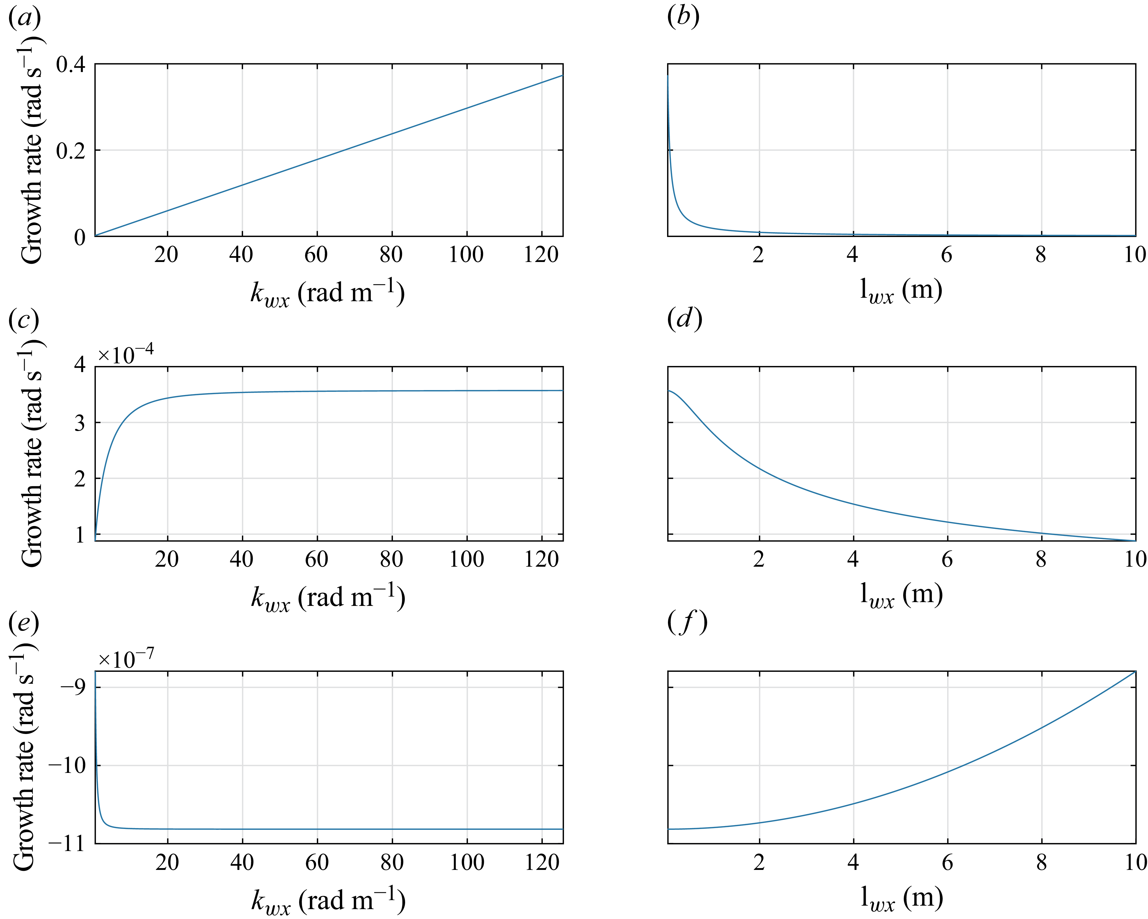
Figures 2(a) and 2(b) show the maximum growth rate of the eigenvalues of the original two-dimensional active-layer model in terms of wavenumber and wavelength, respectively. Matrix
 $\boldsymbol{M}_0$
is built and the eigenvalues are numerically computed. The growth rate for large wavenumbers (i.e. small wavelengths) is positive, indicating that the system of equations is ill-posed. The result is the same when applying the regularisation technique based on the preconditioning mass matrix with
 $\alpha _{\textit{p}}=11.9$
(Chavarrías et al. Reference Chavarrías, Stecca, Siviglia and Blom2019b
) (figures 2
c and 2
d). In contrast, adding a diffusive flux in the streamwise direction to the active-layer model with coefficient equal to
 ${0.15}\,\textrm{m}^{2}\textrm{s}^{-1}$
(the minimum value that regularises this situation) yields a well-posed model (figures 2
e and 2
f). The model is well-posed given that the maximum growth rate is negative as the wavenumber increases. There is a region more easily visible in terms of wavelength in which the growth rate is positive. For transverse wavelengths larger than approximately
 ${2}\,\textrm {m}$
, perturbations grow. This region is associated to growth of alternate bars (Engelund and Skovgaard Reference Engelund and Skovgaard1973; Fredsøe Reference Fredsøe1978; Colombini et al. Reference Colombini, Seminara and Tubino1987; Schielen et al. Reference Schielen, Doelman and de Swart1993).
Growth rate (
 $\textrm{rad s}^{-1}$
) of infinitesimal perturbations as a function of (a, c, e) the wavenumber and (b, d, f) the wavelength for a two-dimensional case (a, b) without regularisation, (c, d) applying a preconditioning mass matrix (PMM) regularisation technique and (e, f) applying diffusion to the active-layer model. Green colours indicate decay of perturbations, while red colours indicate growth of perturbations. For the cases of no regularisation and PMM, the growth rate tends to positive values as the wavenumber increases, indicating that the model is ill-posed. When diffusion is applied, the growth rate tends to negative values as the wavenumber increases, indicating that the model is well-posed. Furthermore, there is a region in which the growth rate is positive (i.e. perturbations grow). This region is associated with the formation of alternate bars.

6.2. Numerical solution
In this section, we model the laboratory experiment described in § 6.1 conducted under conditions in which the active-layer model is ill-posed in two dimensions. To this end, we use Delft3D Flexible Mesh (Deltares 2024), where we have implemented the regularisation strategy consisting of adding a diffusive flux.
The grid is Cartesian with a space steps in streamwise and lateral direction
 $\Delta x = {0.14}\,\textrm {m}$
,
 $\Delta y = {0.05}\,\textrm {m}$
, respectively. In Simulation 1, we do not apply the regularisation strategy. Figure 3 shows the bed elevation along the centre of the flume with time. The situation is ill-posed and a large physically unrealistic wave develops as it occurs when modelling the experiment in one dimension (Chavarrías et al. Reference Chavarrías, Stecca, Siviglia and Blom2019b
). The large oscillation in bed level is accompanied by a sudden fining of the bed surface (figure 4). The growth rate is limited by the shortest wave. As such, and as it is typical in numerical solution of ill-posed models, a refining of the grid would lead to faster-growing oscillations, stressing the fact that these oscillations are not physical.
Simulation 2 is equal to Simulation 1 but for the fact that we apply the diffusion-based regularisation strategy. The diffusion coefficient is equal to
 ${0.15}\,\textrm{m}^{2}\textrm{s}^{-1}$
, which is the minimum amount to regularise this case. We observe that there are no large oscillations neither in bed level (figure 5) nor content of fine sediment in the active layer (figure 6). The fine sediment is gradually entrained into the active layer and transported downstream.
Bed elevation in Simulation 1 (ill-posed, not regularised). Each coloured line represents the bed elevation along the centre of the flume at a given time. Immediately after the start, a large oscillation (more than
 ${0.10}\,\textrm {m}$
considering that the normal flow depth is
 ${0.204}\,\textrm {m}$
) develops.

Volume fraction content of fine sediment in the active layer in Simulation 1 (ill-posed, not regularised). Each coloured line represents the volume fraction content of fine sediment in the active layer along the centre of the flume at a given time. Immediately after the start, a sudden fining of the bed surface occurs as a consequence of the large oscillation in bed level (figure 3) entraining a large amount of fine sediment from the substrate.

Bed elevation in Simulation 2 (well-posed, regularised). Each coloured line represents the bed elevation along the centre of the flume at a given time. No large oscillations develop. The bed erodes gradually following the lowering of the downstream water level.

Volume fraction content of fine sediment in the active layer in Simulation 2 (well-posed, regularised). Each coloured line represents the volume fraction content of fine sediment in the active layer along the centre of the flume at a given time. The fine sediment is gradually entrained into the active layer and transported downstream as the bed erodes.

7. Discussion
7.1. Role of diffusion
The proposed regularisation strategy adds a diffusive flux to the active-layer equation. This additional flux surrogates small-scale processes which are not resolved by the original active-layer equation in a similar fashion as diffusive Brownian motion originates from averaging individual particle motions (Einstein Reference Einstein1905; Pusey Reference Pusey2011). While proving that considering the small-scale motion is essential for obtaining a well-posed model under certain circumstances, we have not derived the diffusive flux from an advective one. Such a derivation would provide a closure relation for the diffusivity as well as a profound theoretical basis. Lacking such a derivation, we observe that the necessary amount of diffusion for regularising the model of the laboratory experiment (
 $\kappa _{\textit{H}}=0.15\,\textrm{m}^2\textrm{s}^{-1}$
) can be expressed as the product of a length scale related to mixing sediment waves
 $L={0.5}\,\textrm{m}$
(as observed by Chavarrías et al. (Reference Chavarrías, Stecca, Siviglia and Blom2019b
)) and a velocity scale related to sediment particle motion
 $v={0.3}\,\textrm{ms}^{-1}$
(in the order of magnitude predicted with the closure relations employed by Chavarrías et al. (Reference Chavarrías, Arkesteijn and Blom2019c
)). This scaling strengthens the idea that the diffusive flux originates from filtering the mixing caused by the waves observed in the experiment.
For an application in which no data is available to estimate the diffussivity, the particle velocity can, as we have done, be derived from closure relations (e.g. Fernandez-Luque and van Beek Reference Fernandez-Luque and van Beek1976). No such relation exists for the length scale of the mixing waves, but it is safe to assume that these scale with the flow depth. In the case of the laboratory experiments, between 2 and 3 times the flow depth.
For a two-size-fractions case, the minimum diffusion coefficient necessary to regularise the model can be computed analytically by setting the growth rate in (5.14) to zero. Depending on a discriminant, an explicit expression is found in (5.20) which can always be used as a first estimate of the necessary diffusion coefficient in practical applications. For cases with more size fractions, the minimum diffusion coefficient can be obtained numerically by computing the eigenvalues of matrix
 $\boldsymbol{M}_0$
and adjusting the diffusion coefficient until the maximum growth rate is zero.
In numerical simulations, the discretisation of the equations introduces numerical diffusion. This numerical diffusion could already regularise the model in some cases. However, numerical diffusion depends on the employed discretisation scheme and grid resolution. Ill-posedness will eventually manifest as the grid is refined. As such, relying on numerical diffusion is not a viable option, but it is relevant to consider it for preventing over-diffusion. Approaches for estimating numerical diffusion exist (LeVeque Reference LeVeque2004) and these could be used to decrease the physical diffusion coefficient accordingly.
Turbulent diffusion in the flow equations (i.e. due to depth-averaged normal turbulent stresses) has been neglected in the analysis. This process plays a crucial role in stabilising the shallow water equations under supercritical conditions (Balmforth and Vakil Reference Balmforth and Vakil2012). Langham et al. (Reference Langham, Woodhouse, Hogg and Phillips2021) conduct a thorough analysis of the one-dimensional unisize morphodynamic model and showed that when bedload is neglected (i.e. all transport occurs in suspension), the model is ill-posed for
 $\textit{Fr}=1$
and turbulent viscosity regularises it. Indeed, the origin of ill-posedness in their case is the resonance between the morphodynamic and hydrodynamic modes, and including turbulent viscosity breaks such a resonance. In our case, we consider bedload transport and Langham et al. (Reference Langham, Woodhouse, Hogg and Phillips2021) showed that when a small amount of bedload is included, the model is well-posed even at
 $\textit{Fr}=1$
and turbulent viscosity is not necessary, as similarly concluded by Lanzoni et al. (Reference Lanzoni, Siviglia, Frascati and Seminara2006) and Cordier et al. (Reference Cordier, Le and de Luna2011). For this reason, we do not expect turbulent viscosity to play a significant role in regularising the active-layer model. Furthermore, the numerical simulations of § 6 include a background turbulent viscosity of
 ${0.1}\,\textrm{m}^{2}\textrm{s}^{-1}$
and still the model is ill-posed without the proposed regularisation strategy.
Ill-posedness in the case we consider stems from the assumptions in the active-layer model and happens for all Froude numbers. Turbulent viscosity could be included in the analysis by adding viscous terms to the momentum equations and building matrix
 $\boldsymbol{M}_0$
accordingly. The analytical obtention of eigenvalues complicates substantially. Nevertheless, exploratory numerical evaluation has been performed over a range of cases and, as expected, turbulent viscosity does not appear to regularise the model (not shown). While this is not a proof, it supports the idea that the problem of ill-posedness of the active-layer model is somehow decoupled from the flow model.
7.2. Role of substrate composition
The problem of ill-posedness has been related to the ‘crossing of eigenvalues’ (Sieben Reference Sieben1997; Stecca et al. Reference Stecca, Siviglia and Blom2014), a condition in which the eigenvalue carrying mostly bed level information (i.e. the bed eigenvalue) and the eigenvalue carrying mostly sediment sorting information (i.e. the sorting eigenvalue) have the same speed. Indeed, the regularisation strategy based on the preconditioning mass matrix (Chavarrías et al. Reference Chavarrías, Stecca, Siviglia and Blom2019b ) aims at preventing this crossing by modifying the celerity of the sorting wave. Colombini and Carbonari (Reference Colombini and Carbonari2020) studied the stability of the one-dimensional active-layer model finding that, in a two-size fraction case, two modes of instability are present: one associated with the modification of bedforms by mixed-size sediment (Livesey et al. Reference Livesey, Ashworth, Bennett and Best1998) and the other associated with the formation of bedload sheets (Whiting et al. Reference Whiting, Dietrich, Leopold, Drake and Shreve1988; Iseya and Ikeda Reference Iseya and Ikeda1987; Recking et al. Reference Recking, Frey, Paquier and Belleudy2009). Their work is pivotal in clearly making this distinction mathematically, as it is difficult to distinct the modes in nature. They derived an order of magnitude of the bed and sorting celerities, and no ill-posedness arises when these become similar in magnitude.
To reconcile this apparent contradiction, we remark that there is a key difference between the analysis carried out by Colombini and Carbonari (Reference Colombini and Carbonari2020) and the one we conduct. They consider that the sediment at the interface between the active layer and the substrate has the same composition as the sediment in the active layer (
 $f^{\textit{I}}_{k}=F_{\textit{a}k}$
). This assumption removes the main factor responsible for ill-posedness (Ribberink Reference Ribberink1987; Stecca et al. Reference Stecca, Siviglia and Blom2014; Chavarrías et al. Reference Chavarrías, Stecca and Blom2018). It is when the active layer is coarser than the substrate that the model is likely to be ill-posed. We recall here the analysis by Chavarrías et al. (Reference Chavarrías, Stecca and Blom2018) also on the one-dimensional active-layer model. The model is ill-posed when
 $\lambda _{\textit{b}}^2-\lambda _{\textit{sc}1}^2+4\lambda _{\textit{b}}\lambda _{\textit{sc}1}\gamma _{1}/\mu _{1,1}\lt 0$
, where
 $\lambda _{\textit{b}}$
is the approximated bed eigenvalue and
 $\lambda _{\textit{sc}1}$
is the approximated sorting eigenvalue. This condition can only be fulfilled when
 $\gamma _{1}\lt 0$
, which occurs mainly when the active layer is coarser than the substrate. Hence, a similar order of magnitude of the bed and sorting celerities is a necessary but not sufficient condition for ill-posedness, and our analysis complements that by Colombini and Carbonari (Reference Colombini and Carbonari2020).
7.3. Role of gravity in sediment transport
Colombini and Carbonari (Reference Colombini and Carbonari2020) also show that considering the effect of gravity in sediment transport (i.e. the effect of the bedslope in modifying the direction and magnitude of sediment transport) is a necessary condition to obtain a cutoff wavenumber above which perturbations decay. Otherwise, the model is regular in the sense of Birkhoff (Reference Birkhoff1954), but cannot represent a natural physical process (see § 4). Our analysis includes the effect of gravity in sediment transport, but in a different way as they do. In our case, gravity rotates the vector downslope without modifying its magnitude (A3). Note that matrix
 $\boldsymbol{D}_{\textit{x}0}=0$
. In their case, the effect of gravity is included by modifying the critical Shields (Reference Shields1936) stress, which slightly modifies the magnitude of the sediment transport. It is possible that their model for including the effect of gravity also yields a cutoff wavenumber and hence also regularises (in our sense) the system of equations. Nevertheless, we are inclined to think that a different type of physics is to be included to obtain a realistic cutoff wavenumber. From (5.20), we see that the necessary amount of diffusion depends on the composition of the substrate (through
 $\gamma _{\textit{x}1}$
), which is in line with the idea that it models the mixing caused by sediment waves, whose characteristics will depend on the substrate composition. The diffusion we add to the active-layer model considers a different process than the effect of gravity in sediment transport.
An analytical proof or a useful expression appears to be difficult to obtain, as new terms arise in matrix
 $\boldsymbol{M}_0$
when including the longitudinal effect of gravity in sediment transport. Nevertheless, we conduct two exercises to gain empirical understanding. A closure relation to include the longitudinal effect of gravity in sediment transport exists in Delft3D (A9), which is not the same as the one employed by Colombini and Carbonari (Reference Colombini and Carbonari2020), but it serves the purpose of this exercise as the physical process that it models is the same. Our closure relation has a parameter
 $\sigma$
[-] that controls the ability of the longitudinal slope in modifying the sediment transport. A value of
 $\sigma =0$
indicates that the longitudinal slope is not considered and a physically realistic value is of order 1.
We conduct numerical simulations of the case presented in § 6 without regularisation, but including the longitudinal effect of gravity in sediment transport. Figure 7 shows the bed elevation after
 ${30}\,\textrm {min}$
of simulation for varying values of parameter
 $\sigma$
. When the longitudinal effect of gravity is not included (
 $\sigma =0$
, the same reference simulation as in § 6.2), a large oscillation develops. Increasing the value of
 $\sigma$
smooths the solution and decreases the amplitude of the wave, but an unrealistically large value (
 $\sigma =100$
) is necessary to prevent the development of large oscillations.
Bed elevation for varying factor
 $\sigma$
of the longitudinal effect of gravity in sediment transport (see (A9)) after
 ${30}\,\textrm {min}$
of simulation. Immediately after the start, a large oscillation (more than
 ${0.10}\,\textrm {m}$
considering that the normal flow depth is
 ${0.204}\,\textrm {m}$
) develops when the effect of the longitudinal gravity is not included. Increasing the value of
 $\sigma$
smooths the solution, but an unrealistically large value (
 $\sigma =100$
) is necessary to prevent the development of large oscillations.

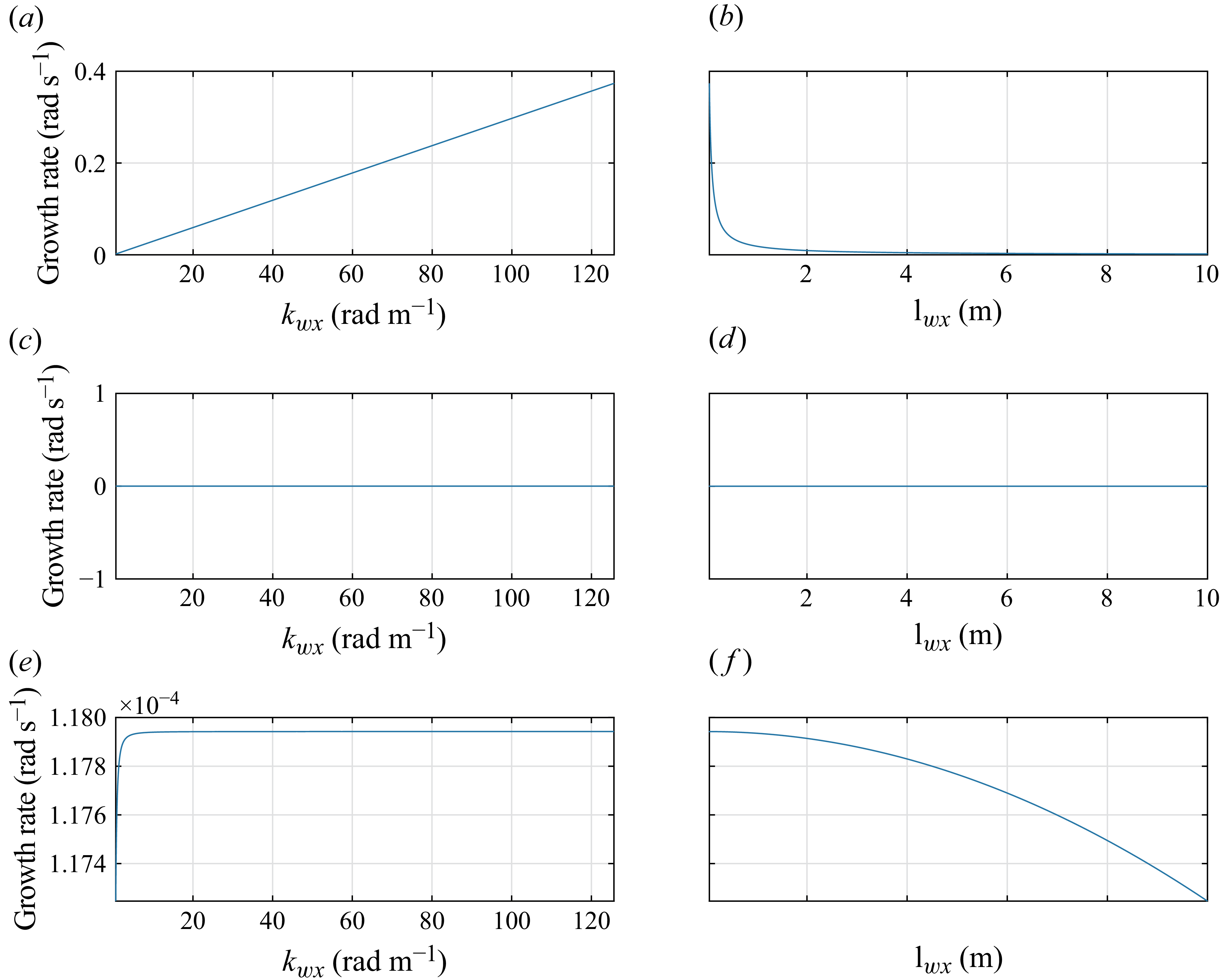
As a second exercise, we implement the longitudinal effect of gravity in the routine to numerically compute the eigenvalues and evaluate the growth rate of perturbations. Figure 8 shows the growth rate of perturbations for the case without longitudinal effect of gravity in sediment transport (
 $\sigma =0$
), including the longitudinal effect of gravity with a physically realistic parameter (
 $\sigma =1$
) and using an unrealistically large parameter (
 $\sigma =100$
). For all cases, perturbations grow for all wavenumbers. We see that increasing the value of
 $\sigma$
decreases the growth rate of perturbations, which is what is to be expected from adding a diffusive flux in the streamwise direction. However, the effect is not strong enough to regularise the model for realistic values of
 $\sigma$
. Hence, including the longitudinal effect of gravity in sediment transport does not regularise the model, which confirms the results from numerical simulations.
Growth rate (
 $\textrm{rad s}^{-1}$
) of infinitesimal perturbations as a function of (a, c, e) the wavenumber and (b, d, f) the wavelength for a two-dimensional case (a, b) without longitudinal effect of gravity in sediment transport (same case as in figures 2
a and 2
b), (c, d) including the longitudinal effect of gravity in sediment transport with a physically realistc parameter
 $\sigma =1$
(see (A9)) and (e, f) using an unrealistically large parameter for the longitudinal effect of gravity
 $\sigma =100$
. Green colours indicate decay of perturbations, while red colors indicate growth of perturbations. For all cases, perturbations grow for all wavenumbers.

While lacking an analytical proof, the two exercises suggest that ill-posedness in the active-layer model is due to lacking other physics than the longitudinal effect of gravity in sediment transport. The regularisation strategy based on adding a diffusive flux to the active-layer equation appears to be necessary to obtain a well-posed model.
7.4. Other regularisation techniques
There could be other techniques that equally regularise the two-dimensional active-layer model from another perspective. Fernández Nieto (Reference Fernández Nieto2003) uses friction to regularise the two-layer shallow water model (the same method is employed by Castro Díaz et al. (Reference Castro Díaz, Nieto, González Vida and Parés Madroñal2011) which is available in English). This model becomes ill-posed when the layers flow at an excessively distinct velocity (Long Reference Long1956; Armi Reference Armi1986; Lawrence Reference Lawrence1990). Fernández Nieto (Reference Fernández Nieto2003) discretises the system of equations of the inviscid problem (no friction). Then, a predictor–corrector strategy is followed. First, a standard numerical scheme (e.g. Lax–Wendroff) is used to obtain an approximation of the solution at time
 $t^{n+1-}$
(predictor). If there is a complex eigenvalue in the system matrix (i.e. the problem is ill-posed), in the corrector step, a friction term is added:
 \begin{equation} S_{q1}=-\frac {1}{\Delta t}\left (\frac {u_1-u_2}{\sqrt {g\left (h_1+h_2\right )}}-1\right )\left (u_1-u_2\right ) , \end{equation}
where
 $_{q1}$
refers to the term of the momentum equation of layer 1,
 $\Delta t$
 $[\textrm {s}]$
is the time step,
 $u_i$
 $[\textrm{ms}^{-1}]$
is the flow velocity of layer
 $i$
and
 $h_i$
 $[\textrm {m}]$
is the flow depth of layer
 $i$
. Note that friction depends on the time step, which is physically unrealistic. In the continuous limit, the necessary friction to regularise the model becomes infinite. Their strategy regularises the discrete (i.e. numerical) system of equations, but not the continuous one. We advocate for strategies with a physical background not only because of their theoretical strength, but also because these are independent of the employed numerical technique.
7.5. Generality of the regularisation by diffusion
In § 5, it has been explained why, mathematically, the regularisation technique based on preconditioning that regularised the one-dimensional model (Chavarrías et al. Reference Chavarrías, Stecca, Siviglia and Blom2019b
) does not regularise the two-dimensional model. We here reconsider this surprising result. The analysis by Chavarrías et al. (Reference Chavarrías, Stecca, Siviglia and Blom2019b
) was conducted on the frictionless one-dimensional model. Indeed, in the same way as without considering friction, diffusion does not regularise the one-dimensional model (§ 5.3), the preconditioning technique would not regularise the one-dimensional model with friction. This can be seen in figure 2 in the limit
 $k_{w\textit{y}}=0$
and in figure 9. As the wavenumber tends to infinity, the growth rate tends to infinite if the model is not regularised, tends to a positive value when applying the preconditioning technique and tends to a negative value when applying diffusion.
Growth rate of infinitesimal perturbations as a function of (a, c, e) the wavenumber and (b, d, f) the wavelength for a one-dimensional case (a, b) without regularisation, (c, d) applying a preconditioning mass matrix (PMM) regularisation technique and (e, f) applying diffusion to the active-layer model. Without regularisation, the growth rate increases indefinitely as the wavenumber increases, indicating that the model is ill-posed. When applying PMM, the growth rate tends to a positive value indicating that the model is ill-posed. When applying diffusion, the growth rate tends to a negative value as the wavenumber increases, indicating that the model is well-posed.

The results by Chavarrías et al. (Reference Chavarrías, Stecca, Siviglia and Blom2019b
) are recovered when friction is neglected (figure 10). Using the preconditioning technique yields purely real eigenvalues (i.e. the growth rate is equal to 0 and the model is well-posed). When adding diffusion, the maximum growth rate tends to a value slightly lower than
 ${1.1913\times 10^{-4}}\,\textrm{rad}\,\textrm{s}^{-1}$
, which is the value predicted using (5.25). The discrepancy is due to the fact that the numerical obtention of eigenvalues is done using the fully unsteady model, while (5.25) is derived assuming quasi-steady flow.
Growth rate of infinitesimal perturbations as a function of (a, c, e) the wavenumber and (b, d, f) the wavelength for an inviscid (i.e. frictionless) one-dimensional case (a, b) without regularisation, (c, d) applying a preconditioning mass matrix (PMM) regularisation technique and (e, f) applying diffusion to the active-layer model. Without regularisation, the growth rate increases indefinitely as the wavenumber increases, indicating that the model is ill-posed. When applying PMM, the growth rate is equal to 0, indicating that the model is well-posed. When applying diffusion, the growth rate tends to a positive value as the wavenumber increases, indicating that the model is ill-posed.

Interestingly, numerical simulations employing the one-dimensional viscous model regularised with the preconditioning technique (which we see here it is ill-posed) yield no oscillations in the solution, suggesting the case is well-posed (Chavarrías et al. Reference Chavarrías, Stecca, Siviglia and Blom2019b , Reference Chavarrías, Arkesteijn and Blomc ). This indicates that numerical diffusion was sufficient to dampen the growth of the high-wavenumber perturbations. Note that, in contrast to the case without regularisation, the growth rate is positive, but bounded when applying the preconditioning technique (figures 9 c and 9d), and it is a much smaller value than without regularisation.
Diffusion in the active-layer model appears to regularise both the one-dimensional and two-dimensional models proving to be a more general solution. There are still reasons for using the preconditioning technique in the one-dimensional model as it is computationally less expensive (no diffusive terms need to be discretised and solved) and can be easily implemented in existing morphodynamic models. The preconditioning parameters need to be estimated, but the same applies to the diffusion coefficient. While the preconditioning technique is well-posed in the sense of Birkhoff (Reference Birkhoff1954) (i.e. there is a finite upper bound to the growth rate) and has proven to give physically realistic results, diffusion yields a more physical solution as perturbations decay for large wavenumbers.
Furthermore, one important limitation of the pre-conditioning based regularisation for the one-dimensional model is that it can only be used when the active-layer thickness is constant (Chavarrías et al. Reference Chavarrías, Stecca, Siviglia and Blom2019b ). This limitation originates from the fact that the summation of all the active-layer equations for each grain size (with the preconditioning factor) must be equal to the Exner equation. We do not foresee such a limitation for the diffusion-based regularisation here proposed. Nevertheless, the effect of using specific closure relations for the active-layer thickness could be assessed by linearising such a relation and introducing it into the system of equations.
In a similar manner, other simplifying assumptions could be relaxed. For instance, we have assumed that the friction coefficient is independent on the flow depth and grain size. We do not expect that the domain of ill-posedness and the effect of the regularisation technique significantly depends on this assumption. This is because ill-posedness stems from the simplifications inherent to the active-layer model in combination with capacity sediment-transport models. While obtaining analytical results when including more complex friction relations becomes prohibitive, exploratory numerical analysis is possible.
7.6. Linear analysis and nonlinear problem
The linear stability analysis performed in this work to study the well-posedness of the active-layer model is based on infinitesimal plane-wave (i.e. continuous and smooth) perturbations around a uniform reference state (i.e. flat bed). This is the common approach in the literature for all sorts of different physical models, as it makes the problem tractable (Whitham Reference Whitham1974; Courant and Hilbert Reference Courant and Hilbert1989; Fitt Reference Fitt1989; Joseph and Saut Reference Joseph and Saut1990; Ribberink Reference Ribberink1987; Gray Reference Gray1999; Cordier et al. Reference Cordier, Le and de Luna2011; Stecca et al. Reference Stecca, Siviglia and Blom2014; Langham et al. Reference Langham, Woodhouse, Hogg and Phillips2021). Formally, the conclusions drawn from the linear analysis may not extend to the nonlinear regime. Suppose a case with well-developed river bars in which nonlinear modes are non-negligible (Colombini et al. Reference Colombini, Seminara and Tubino1987; Schielen et al. Reference Schielen, Doelman and de Swart1993). We believe it is theoretically possible that local conditions at the linear level yield a well-posed or ill-posed model, but the opposite happens when considering nonlinear modes. Nevertheless, we are not aware of any example in the literature in which this is studied and we are uncertain about how exactly this analysis could be conducted. The same logic applies to the regularisation strategy. Studying the linear system is the common approach to regularise ill-posed systems and proves to be succesful in the nonlinear regime (Gray Reference Gray1999; Langham et al. Reference Langham, Woodhouse, Hogg and Phillips2021; Chavarrías et al. Reference Chavarrías, Stecca, Siviglia and Blom2019b ), although there is no formalism at the nonlinear level. A hint that the linear analysis extends to the nonlinear regime is found in studying the stability of numerical schemes. The stability of numerical schemes is typically studied at the linear level by means of von Neumann and Richtmyer (Reference von Neumann and Richtmyer1950) analysis and the conclusions can be extended to the nonlinear regime provided that the solution is sufficiently smooth (Strang Reference Strang1964; Tadmor Reference Tadmor2012).
8. Conclusions
The model that considers mixed-size sediment in morphodynamic processes (i.e. the active-layer model) may be ill-posed under certain circumstances. When the model is ill-posed, it loses its predictive capabilities, as it is unstable to short-wave perturbations and the solution does not converge when the numerical grid is refined. Chavarrías et al. (Reference Chavarrías, Stecca, Siviglia and Blom2019b ) devised a regularisation strategy to guarantee that the inviscid one-dimensional model is well-posed. We show that the extension to two dimensions of that strategy does not regularise the two-dimensional version of the active-layer model.
We propose a different regularisation strategy for the two-dimensional model and we prove analytically that it yields an unconditionally well-posed model. This second strategy is based on adding a diffusive flux to the active-layer equation which considers mixing processes occurring at a small scale not resolved by the model. We also show that this strategy regularises the one-dimensional model as well.
We implement the regularisation strategy in Delft3D Flexible Mesh and successfully use it to regularise a model representing a laboratory experiment conducted under conditions in which the active-layer model is ill-posed. While the non-regularised simulation presents physically unrealistic oscillations, the regularised simulation remains stable.
Acknowledgements
The author would like to thank the editor Dr N. Balmforth and three anonymous reviewers for their very useful comments that significantly improved the manuscript. The author also acknowledges useful discussions with Dr Annunziato Siviglia.
Declaration of interests
The author reports no conflict of interest.
Appendix A. Sediment transport closure relation
We use the non-dimensional sediment transport closure relation by Ashida and Michiue (Reference Ashida and Michiue1971):
 \begin{equation} q^*_{\textit{b}k}=A\left (\theta _k-\xi _k\theta _{\textit{c}}\right )\left (\sqrt {\theta _k}-\sqrt {\xi _k\theta _{\textit{c}}}\right ) \quad \forall k , \end{equation}
where
 $A=17$
[
 $-$
] is a non-dimensional coefficient,
 $\theta _{\textit{c}}=0.05$
[
 $-$
] is the non-dimensional critical shear stress and
 $\xi _{k}$
[
 $-$
] is the hiding-exposure function:
 \begin{equation} \xi _k=\left \{\!\! \begin{array}{l l} 0.8429\left (\dfrac {d_{k}}{D_{\textit{m}}}\right )^{-1} & \quad \text{for } \dfrac {d_{k}}{D_{\textit{m}}}\leq 0.38889,\\[8pt] \left (\dfrac {\log _{10}(19)}{\log _{10}\left(19\dfrac {d_{k}}{D_{\textit{m}}}\right)}\right )^{2} & \quad \text{for } \dfrac {d_{k}}{D_{\textit{m}}}\gt 0.38889,\\ \end{array} \right . \ \;\forall k. \end{equation}
The hiding-exposure function models the fact that fine sediment is less exposed to the flow when being in a mixture as it hides behind large grains and vice versa (Einstein Reference Einstein1950). The hiding factor depends on the mean grain size of the bed surface
 $D_{\textit{m}}$
[
 $-$
] which can be computed as the arithmetic or the geometric mean grain size (see the following).
Using (2.8), one computes the magnitude of the bedload transport rate for each size fraction
 $q_{\textit{b}k}$
 $[\textrm{m}^{2}\,\textrm{s}^{-1}]$
based on the result of (A1).
The direction of the sediment transport (
 $\varphi _{\textit{s}k}$
 $[\textrm {rad}]$
) reads (van Bendegom Reference van Bendegom1947)
 \begin{equation} \tan {\varphi _{\textit{s}k}}=\frac {q_{\textit{y}}- \frac{1}{g_{\textit{s}k}}\frac{\partial \eta }{\partial y}}{q_{\textit{x}}-\frac{1}{g_{\textit{s}k}}\frac{\partial \eta }{\partial x}}, \quad k\in \{1,N\} , \end{equation}
where
 $g_{\textit{s}k}$
[
 $-$
] is (Koch and Flokstra Reference Koch and Flokstra1980; Talmon et al. Reference Talmon, Struiksma and Mierlo1995)
 \begin{equation} g_{\textit{s}k}=A_{\textit{s}}\theta _k^{B_{\textit{s}}}, \quad k\in \{1,N\} , \end{equation}
where
 $A_{\textit{s}}$
[
 $-$
] and
 $B_{\textit{s}}$
[
 $-$
] are non-dimensional parameters (see, for instance, Baar et al. (Reference Baar, de Smit, Uijttewaal and Kleinhans2018) for a review).
Using (A3), the rotated bedload transport components
 $q_{\textit{brx}k}$
 $[\textrm{m}^{2}\,\textrm{s}^{-1}]$
and
 $q_{\textit{bry}k}$
 $[\textrm{m}^{2}\,\textrm{s}^{-1}]$
read
 \begin{align}& q_{\textit{brx}k}=q_{\textit{b}k} \cos {\varphi _{\textit{s}k}}, \quad k\in \{1,N\} , \end{align}
 \begin{align}& q_{\textit{bry}k}=q_{\textit{b}k} \sin {\varphi _{\textit{s}k}}, \quad k\in \{1,N\} . \end{align}
Equation (A3) rotates the sediment transport direction downslope without modifying its magnitude. For considering the effect of the bed slope on the transport in the longitudinal direction, Talmon et al. (Reference Talmon, Struiksma and Mierlo1995) proposed
 \begin{align}& q_{\textit{bx}k}=\varsigma _k q_{\textit{brx}k}, \quad k\in \{1,N\} , \end{align}
 \begin{align}& q_{\textit{by}k}=\varsigma _k q_{\textit{bry}k}, \quad k\in \{1,N\} , \end{align}
where
 $\varsigma _k$
[
 $-$
] is defined as
 \begin{equation} \varsigma _k=1-\sigma \left .\frac {\partial \eta }{\partial s}\right |_k, \quad k\in \{1,N\} , \end{equation}
where
 $({\partial\eta}/{\partial s})|_k$
[
 $-$
] denotes the longitudinal bed slope direction for the sediment transport of size fraction
 $k$
and
 $\sigma$
[
 $-$
] is a non-dimensional parameter (typically
 $\sigma =1$
).
The longitudinal bed slope reads
 \begin{equation} \left .\frac {\partial \eta }{\partial s}\right |_k=\frac {\partial \eta }{\partial x}\cos {\varphi _{\textit{s}k}}+\frac {\partial \eta }{\partial y}\sin {\varphi _{\textit{s}k}}, \quad k\in \{1,N\} , \end{equation}
and is limited to a maximum value related to the angle of repose
 $\phi =30^\circ$
 $[\textrm {deg}]$
:
 \begin{equation} \left .\frac {\partial \eta }{\partial s}\right |_{k\textit{max}}=0.9\tan {\phi } . \end{equation}
The longitudinal bed slope effect is not considered by setting
 $\sigma =0$
. This correction is not considered in the analytical results of this work for the sake of simplicity and its effect is studied in the discussion.
The derivative of the sediment transport relation with respect to the non-dimensional bed shear stress is
 \begin{equation} \frac {\partial q^*_{\textit{b}k}}{\partial \theta _k}=A\left [\frac {\left (\theta _k-\xi _k\theta _{\textit{c}}\right )}{2\sqrt {\theta _k}}+\left (\sqrt {\theta _k}-\sqrt {\xi _k\theta _{\textit{c}}}\right ) \right ] \quad \forall k . \end{equation}
The derivative of the sediment transport relation with respect to the hiding function is
 \begin{equation} \frac {\partial q^*_{\textit{b}k}}{\partial \xi _k}=\frac {-A\theta _{\textit{c}}}{2}\left [\frac {\left (\theta _k-3\xi _k\theta _{\textit{c}}\right )}{\sqrt {\xi _k\theta _{\textit{c}}}}+2\sqrt {\theta _k} \right ] \quad \forall k . \end{equation}
The derivative of the hiding function with respect to the mean grain size is
 \begin{equation} \frac {\partial \xi _k}{\partial D_{\textit{m}}}=\left \{\!\! \begin{array}{l l} \dfrac {0.8429}{d_k} & \quad \text{for } \dfrac {d_{k}}{D_{\textit{m}}}\leq 0.38889,\\[8pt] \dfrac {2\left (\log _{10}(19)\ln (10)\right )^2}{D_{\textit{m}}\left [\ln \left (\frac{19d_k}{D_{\textit{m}}}\right )\right ]^3} & \quad \text{for } \dfrac {d_{k}}{D_{\textit{m}}}\gt 0.38889,\\ \end{array} \right . \ \; \forall k. \end{equation}
The arithmetic mean grain size is
 \begin{equation} D_{\textit{m}}=\sum _{k=1}^{N}F_{\textit{a}k}d_k=d_N+\sum _{k=1}^{N-1}F_{\textit{a}k}\left (d_k-d_N\right ) . \end{equation}
The expression on the right-hand side of (A15) considers the constraint in (2.7).
The derivative with respect to the volume fraction content of sediment in the active layer is
 \begin{equation} \frac {\partial D_{\textit{m}}}{\partial F_{\textit{a}l}}=d_l-d_N, \quad l\in [1,N-1]. \end{equation}
The geometric mean grain size is
 \begin{equation} D_{\textit{m}}=d_{\textit{ref}}2^{-\phi _{\textit{m}}} , \end{equation}
where
 $\phi _{\textit{m}}$
[
 $-$
] denotes the geometric mean grain size in
 $\phi$
-scale:
 \begin{equation} \phi _{\textit{m}}=\sum _{k=1}^{N}\phi _kF_{\textit{a}k} , \end{equation}
where
 $\phi _k$
denotes the grain size
 $k$
in
 $\phi$
-scale:
 \begin{equation} \phi _k=-\log _2\left (\frac {d_k}{d_{\textit{ref}}}\right ) . \end{equation}
Parameter
 $d_{\textit{ref}}$
[
 $\textrm {m}$
] denotes a reference grain size (e.g.
 $d_{\textit{ref}}={1}\,\textrm {mm}$
) to obtain the right dimensions.
In terms of the dependent variables of the model and accounting for the constrain in (2.7), the geometric mean grain size is
 \begin{equation} D_{\textit{m}}=d_{\textit{ref}}2^{\log _2\left (\tfrac{d_N}{d_{\textit{ref}}}\right )+\sum _{k=1}^{N-1}F_{\textit{a}k}\log _2\left (\tfrac{d_k}{d_N}\right )} . \end{equation}
The derivative with respect to the volume fraction content of sediment in the active layer is
 \begin{equation} \frac {\partial D_{\textit{m}}}{\partial F_{\textit{a}l}}=d_N\ln (2)\log _2\left (\frac {d_l}{d_N}\right )\prod _{k=1}^{N-1}\left (\frac {d_k}{d_N}\right )^{F_{\textit{a}k}}, \quad l\in [1,N-1]. \end{equation}