1. Introduction

The purpose of this article is to show a precise sense in which quantum mechanics can explain the success of classical mechanics through the classical $\hslash \to 0$ limit. This work is a contribution to a tradition of philosophical investigations of the classical limit stemming from Post (Reference Post1971) and continuing through Scheibe (Reference Scheibe1986), Rohrlich (Reference Rohrlich1990), Radder (Reference Radder1991), and Primas (Reference Primas1998). A central question in these investigations is whether one can use quantum mechanics to explain not only why the predictions of classical mechanics are nearly accurate in many systems but also why the theoretical structure of classical mechanics is successful in generating predictions and explanations of phenomena. The contribution of the current investigation is to show that one can produce an explanation of the theoretical structure of classical mechanics from quantum mechanics through the classical limit. The explanation proceeds by showing that the theoretical properties and relations of physical magnitudes as represented in quantum mechanics can always be understood as “close” to the theoretical properties and relations as represented in classical mechanics. I aim to show that the classical $\hslash \to 0$ limit makes the notion of “closeness” precise. What it means for physical magnitudes to be “close” is that their difference lies within an error bound determined by both a numerical value and a system of units in which that numerical value is expressed. The system of units in turn is encoded as a choice of numerical value for Planck’s constant $\hslash$, understood as the same physical parameter in different units, on the way to the limit. Although changing units (as $\hslash \to 0$) does not affect either the phenomenon being modeled or the theory used to model it, it can encode larger error bounds in which quantum and classical mechanics become “close.”

This notion of “closeness” or “approximation” is already employed in mathematical physics, and I believe it is implicit in discussions in the broader physics community. It is worth making this interpretation explicit, however, because the notion of “closeness” is considerably stronger than that recognized in most conceptual discussions. My analysis entails that the predictions given by quantum mechanics for expectation values in each state are “close” to the corresponding predictions in classical physics. But it also provides much more: (i) the error bounds by which the predictions of quantum and classical mechanics are allowed to differ can be made uniform for all possible states, and (ii) the properties and relations encoded in the algebraic structure of quantum mechanics can be shown to be close to the properties and relations encoded in the algebraic structure of classical mechanics.

I believe the significance of the $\hslash \to 0$ limit goes beyond establishing the relationship between quantum and classical mechanics. Through this investigation, we can clarify our interpretation of quantities, propositions, and other theoretical structure in quantum theories. Further, I believe an interpretation of the classical limit is important for understanding its role in the stage of heuristics, or theory construction. And finally, I hope it will become clear that the notion of “approximation on certain scales” I develop is not unique to the classical limit; this concept appears elsewhere in quantum physics. For example, I believe the interpretation developed here has implications for our understanding of renormalization in quantum field theories, where one also speaks of “approximation on certain scales.” These last two topics of heuristics and renormalization go beyond the current work and I will not discuss them further, but these potential applications show that the current topic can lay the groundwork for future investigations.

The structure of the article is as follows. In section 2, I review the perspectives of other authors on the explanatory status of the classical limit. I show how the old question of whether the classical limit allows one to explain the theoretical structure of classical mechanics arises again in the context of work by contemporary authors. In section 3, I lay out mathematical tools for understanding the classical limit of quantum theories in terms of continuous fields of algebras, which gives rise to the theory of strict deformation quantization. I then use these mathematical tools in section 4 to make precise how one can explain through the classical limit why quantum systems behave approximately classically when probed on certain scales. Finally, I conclude in section 5 with some discussion.

2. Background

This section situates the position developed in this article within the contemporary literature on the classical limit, primarily in response to recent work by Rosaler (Reference Rosaler2015a, Reference Rosaler2015b, Reference Rosaler2016, Reference Rosaler2018). I show that Rosaler’s interpretation of the classical limit lacks important features, which I hope to be able to recover in the following sections. In particular, Rosaler is able to explain only the success of the empirical predictions of classical mechanics but not its theoretical structure. This issue is, of course, much older—dating from at least the work of Post (Reference Post1971) and Radder (Reference Radder1991). It is the central concern of this article to show that one can explain the theoretical structure of classical mechanics from quantum mechanics, and so it will be helpful to establish that this is a live issue even though it has not been the focus of contemporary discussions.

Rosaler frames his contribution as a response to Batterman (Reference Batterman1991, Reference Batterman2002), who argues that quantum mechanics fails to explain the success of classical mechanics because of the “singular” nature of the $\hslash \to 0$ limit. For example, Batterman (Reference Batterman2002) constructs a family of quantum states (in the form of wave functions) from the data of a classical theory. These wave functions take the form $\psi \left(q\right)\sim e^{\frac{i}{\hslash }S(q,P)}$, where S is a real-valued function. Batterman claims that since these functions fail to converge in the limit as $\hslash \to 0$, the classical limit is “singular.” This feature shows, according to Batterman, that one must pay careful attention to deviations from classical behavior in the $\hslash \to 0$ limit, which he refers to as semiclassical physics. These nonclassical deviations, Batterman argues, prevent the reduction of classical to quantum mechanics: “My discussion of these borderland phenomena and their explanation should also lead one to question what has become a fairly common sentiment among physicists and philosophers. It seems that most investigators maintain a reductionist and even eliminativist attitude toward classical physics given the many successes of the quantum theory. Of course, it is just this attitude that I have been at pains to question” (111). While I completely agree with Batterman that the semiclassical phenomena he points to—especially those concerning chaotic systems—are important and interesting, I am not convinced that they prevent us from providing a (partial) reduction. In particular, I do not think Batterman’s claims extend to all instances of the $\hslash \to 0$ limit. Perhaps Batterman is correct that a reductive explanation of all aspects of chaotic classical systems is impossible. But I believe that for some systems, it is possible to give a reductive explanation of the success of at least the kinematic structure of classical mechanics from the kinematic structure of quantum mechanics, and I will attempt to establish this in what follows.

Rosaler and I appear to agree about the possibility of giving a kind of reductive explanation of classical behavior, but our proposed explanations differ radically. The explanation I will offer of classical behavior follows Batterman’s approach, at least in the sense that I employ the $\hslash \to 0$ limit. Here, I follow an idea of Nickles (Reference Nickles1973) (which Batterman also cites) that these limiting relations might provide “approximative reductions”: “Approximative reductions … might be said to explain why the predecessor theory worked as well as it did” (185 n. 4). It is precisely this kind of explanation that I will take the classical limit to offer. I believe one can use the classical limit to explain why classical mechanics works as well as it did. In contrast, Rosaler leaves behind the classical $\hslash \to 0$ limit altogether, instead giving an alternative explanation of the success of classical mechanics through decoherence theory. I want to highlight two of the reasons he provides for this approach, which I believe to be ill founded.

First, Rosaler claims there are difficulties interpreting the $\hslash \to 0$ limit because $\hslash$ is a physical constant that takes on a single value: “One may make the predictable criticism that Batterman’s analysis relies on the limit $\hslash \to 0$ even though $\hslash$ is constant for all real systems, and that the relevance of the analysis for real systems is obscured by this fact” (Reference Rosaler2015a, 331). Rosaler seems to believe that these difficulties can be dealt with, but only by making matters more complicated. The common strategy that he points to is outlined already by Batterman: “One might reasonably wonder what it could mean to let a constant change its value. The way to understand ‘ $\hslash \to 0$’ is that it is the limit in which $\hslash$ is small relative to some quantity having the same dimension—namely, the classical action” (Reference Batterman2002, 99 n. 1). However, Rosaler notes, we commonly analyze the behavior of quantum systems as $\hslash$ varies without attention to the ratio between $\hslash$ and the classical action. Rosaler asserts that this “may be seen as a matter of convenience, [but] it is a convenience that comes at a significant cost to our physical insight” (Reference Rosaler2015a, 331). According to him, if we do not explicitly treat the classical limit in terms of ratios of $\hslash$ to classical action, we will not have complete understanding of the intertheory relations between quantum and classical physics.

There seems to be an implicit assumption in Rosaler’s argument here that the only way one might make sense of the $\hslash \to 0$ limit is to employ the strategy of using $\hslash$ as proxy for a dimensionless ratio. Rosaler is not alone on this point; the statement that the constant $\hslash$ cannot vary echoes Nickles, who writes, “Indeed, it makes no physical sense to permit physical constants to vary ( $\hslash \to 0$, $c\to \infty$)” (Reference Nickles1973, 201) and Radder, who writes, “Of course, from a physical point of view putting $h=0$ is impossible: h is an empirically fixed constant unequal to zero” (Reference Radder1991, 209 n. 8).

Although none of these authors elaborates on this impossibility, the reason seems to be that the alternative forces us to imagine different possible worlds in which $\hslash$ really takes a different value and the physics of such worlds differs from our own. I think one might reasonably worry, if this were the alternative, about how one could use facts about these other possible worlds in which $\hslash$ differs to explain anything about our own world.

Fortunately, I do not believe this is the only alternative. I hope to show that it is possible for one to interpret the $\hslash \to 0$ limit as representing features of our own world without thinking of $\hslash$ as proxy for a dimensionless ratio. This is not to say that I reject the dimensionless ratio interpretation; I think such an interpretation works together with the one I will present, and so I return to their relationship briefly in section 5.

Second, Rosaler claims that philosophers who analyze only mathematical relations between theories (like the $\hslash \to 0$ limit) miss important empirical content: “While questions about empirical reduction are partially mathematical in nature, assessing whether one theory reduces empirically to another requires further empirical input regarding the set of circumstances under which the reduced theory furnishes an accurate representation of the behavior of some actual physical system; without such information, it would not generally be possible to assess whether one theory encompasses the domain in which the other is successful” (Reference Rosaler2015a, 338). Rosaler’s preferred notion of empirical reduction is described as follows: “Empirical reduction requires that every circumstance under which the behavior of a real physical system can be modeled in the reduced theory (in this case, classical mechanics) is also one in which that same behavior can be modeled at least as precisely in the reducing theory (in this case, quantum mechanics). That is, empirical reduction requires that the reducing theory wholly subsume the physical domain of applicability of the reduced theory, but does not necessarily require the reduced theory’s formal mathematical structure to be subsumed as a special or limiting case of the reducing theory’s formal structure” (326).

I agree with Rosaler that extra empirical information is necessary to know the situations in which a reduced theory is successful. But I believe his statements here go too far toward what Nagel called an “instrumentalist” approach, according to which “the claim that a theory T … is reduced to another theory T′ [is] that all the observation statements which can be derived from given data with the help of T can also be derived with the help of T′, but not conversely. Accordingly, the question to which this account of … reduction is addressed is not the ostensibly asserted content of the theories involved in reduction, but the comparative ranges of observable phenomena to which two theories are applicable” (Reference Nagel, Curd and Cover1998, 911). Nagel believed the instrumentalist approach was inadequate. He writes, “It ignores the question of how, if at all, the concepts of a reduced theory are related to those of the reducing one, or in what way statements about a variety of observable things may fall within the scope of both theories” (912). Another way of putting the point is that if one only shows that the reducing theory can make all of the correct empirical predictions about the domain of the reduced theory, then one has not given an adequate explanation of why the theoretical structure of the reduced theory was successful. In the case at hand, we have a genuine explanatory task to say why the theoretical apparatus of classical Hamiltonian phase spaces with Poisson brackets is successful when the quantum theory does not employ those mathematical tools.

This issue of whether one can give an explanation of the theoretical structure of classical mechanics from quantum mechanics has been prominent in the literature. For example, Post formulates the requirement of reductive explanations as the “General Correspondence Principle”: “the principle claims far more than mere ‘agreement’ on individual instances of factual data found to be successfully covered by the [reduced theory]. The General Correspondence Principle claims that the [reducing theory] inherits a coherent pattern of theorems, including some higher levels, from the [reduced theory]” (Reference Post1971, 235). Yet, we see a contrasting view from Radder, who claims that the classical limit does not explain the theoretical structure of classical mechanics: “In surveying the whole episode in the history of 20th century physics we may conclude that, ultimately, the success of the correspondence principle appears not to rest upon a conceptual correspondence but rather upon a combination of numerical and formal correspondence” (Reference Radder1991, 208). Later, he writes, “Such a formal correspondence between mathematical equations is by itself insufficient. … The formally corresponding terms or quantities need to have the same experimentally obtainable values in (the neighborhood of) that limit” (212). And again, “The basic problem is that classical observables are mathematically represented by functions (on a phase space of generalized coordinates), while quantum observables are represented by operators (on a Hilbert space of state vectors)” (219). My goal in the remainder of the article is to show that in the case at hand, one can explain the theoretical structure of classical mechanics from quantum mechanics. The explanation I provide will yield exactly what Radder seems to desire and yet asserts is not available.

In fact, I think the explanation Rosaler gives also goes beyond what an instrumentalist would hope for, but it is worth being clear about the explanandum at the outset. In what follows, I aim to provide an explanation of why the kinematic structure of classical mechanics is successful. I will show how classical physics arises as an approximation (and so I go beyond the instrumentalist), and yet my explanation will also satisfy Rosaler’s desideratum by allowing empirical information concerning allowable errors to play a role in explaining when classical mechanics is accurate.

In order to lead us into my positive account of the explanation of classical behavior, I believe it is helpful to pinpoint exactly where in Rosaler’s analysis this issue arises. Ultimately, Rosaler’s association of quantum states with classical states proceeds by identifying a quantum state with the classical state whose definite values for the classical position and momentum quantities are equal to the expectation values for the quantum position and momentum operators. Rosaler’s justification for this is the assumption that “some mechanism for collapse or effective collapse” (Reference Rosaler2015a, 335) will allow us to model a quantum superposition by considering just one component along one of its branches.Footnote ¹ Rosaler is appropriately agnostic about what this mechanism for collapse might be. However, I do not think this dispels the worry.

Suppose, as Rosaler does, that there is some collapse-like mechanism that leads to well-localized wave functions along branches defined by particular coherent “pointer” states. Even so, there is still a question of why one is justified in employing classical concepts to describe these quantum states at all—for example, the notion of a determinate value and a definite trajectory. It is not clear why one should take the expectation values of physical quantities in a quantum state, which do not represent determinate values of those physical quantities in general, and think of them as determinate states in a classical phase space with the structure of a manifold. And furthermore, it is not clear why one can think of the quantum position and momentum operators as corresponding to classical quantities of position and momentum, which are functions on a phase space with Poisson structure. Why can one successfully employ the kinematic framework of classical mechanics to represent a system whose quantum description is in terms of an entirely different kinematic framework?

Rosaler’s analysis using decoherence theory is illuminating, and I believe it is compatible in many ways with what I will say in the rest of this article. I only aim to fill this gap—which is small but conceptually important—in our explanation of classical behavior from quantum mechanics. The next section (sec. 3) reviews the mathematical tools necessary for my analysis, and then section 4 uses an interpretation of these tools to present an explanation of the success of classical kinematics from quantum mechanics.

3. The Classical Limit

Although historically the term “quantization” has been reserved for the process of constructing a quantum theory, modern mathematical theories of deformation quantization are understood instead to provide tools for the “inverse” or “dual” process of taking the classical limit (Rieffel Reference Rieffel1989, Reference Rieffel1993, Reference Rieffel1994; Landsman Reference Landsman1998, Reference Landsman, Butterfield and Earman2007, Reference Landsman2017).Footnote ² This is accomplished by constructing a family of algebras, each representing a quantum theory of the same “form” (i.e., with the capacity to represent the same physical systems), but with a different value for Planck’s constant $\hslash$. As I attempt to make precise later, each of these algebras can be thought of as representing the same system in a different system of units. One provides additional structure to “glue” these algebras together into a continuous field, which allows one to specify continuous limits of states and quantities in the limit as $\hslash \to 0$. There are other limits one might analyze to recover classical behavior (e.g., the limit $N\to \infty$ of an increasing number of particles), but I focus on the $\hslash \to 0$ limit here.

How is the $\hslash \to 0$ limit supposed to explain classical behavior? Imagine starting with a fully quantum theory in which Planck’s constant takes the value $\hslash =1$ in natural units. Next, “zoom out” from the quantum description and look at larger and larger scales, letting Planck’s constant get smaller and smaller until $\hslash \approx 0$. The theory one obtains is an approximate classical description of the same system on the appropriate scales.

This is a nice outline, but given the skepticism of Rosaler and others, we should admit that there are missing pieces. What does it mean to have the same theory of a physical system but “zoom out”? What exactly is a “scale” in this context, and how is it related to a value for $\hslash$? What is the notion of approximation involved, and how does the $\hslash \to 0$ limit capture this process in a way that has explanatory force? It is my goal in section 4 to answer these questions. In order to do so, I will need to use some details of the mathematical tools surrounding deformation quantization, which I now present in this section.

3.1. Continuous Fields of C*-Algebras

In this section, I describe the mathematical tools used to represent the classical limit. I take a quantum theory to be given by a (noncommutative) C*-algebra representing the bounded physical quantities of a system including perhaps generalized position and momentum quantities that satisfy some canonical (anti)commutation relations (see Petz Reference Petz1990; Clifton and Halvorson Reference Clifton and Halvorson2001; Ruetsche Reference Ruetsche2011).Footnote ³ Physicists and philosophers have debated whether C*-algebras are an appropriate starting point for quantum theories or whether we need the additional structure of a Hilbert space representation (see, e.g., Arageorgis Reference Arageorgis1995; Lupher Reference Lupher2008; Ruetsche Reference Ruetsche2011). I ignore these debates in what follows and simply assume that we start with a C*-algebra for a quantum theory; this should be uncontroversial because all parties to these debates agree that we require at least the structure of a C*-algebra (especially for the finite systems considered here).

A C*-algebra already carries enough structure to define a number of topologies (e.g., norm, weak) that provide different notions of the limit of a net of physical quantities within an algebra (see Feintzeig Reference Feintzeig2018c). However, to understand the classical limit, one requires resources for taking the limit of a family of algebras, where each algebra is understood to represent a full quantum theory. Such tools are provided in the theory of strict deformation quantization.

In a strict deformation quantization, one has a family of algebras 𝔄_h for each possible numerical value $h\in [0,1]$ of Planck’s constant $\hslash$. The algebra 𝔄₀ at the value $h=0$ will represent a classical theory, so one requires that 𝔄₀ contains as a norm dense subset a (complex) Poisson algebra (𝒫, {⋅, ⋅}). This Poisson algebra arises from a Hamiltonian formulation of a classical theory, where the elements of 𝒫 are smooth functions on a phase space with the structure of a Poisson manifold and hence can be thought of as physical magnitudes (Landsman Reference Landsman1998). Yet, each algebra 𝔄_h for $h\ne 0$ will be a noncommutative algebra representing a quantum theory.

The core idea of taking the limit of a collection of C*-algebras is to gather them into a structure known as a continuous field of algebras.

Definition 1. A continuous field of C*-algebras ( ${\left({𝔄}_h\right)}_{h\in [0,1]}$, 𝒦) consists in a family of C*-algebras 𝔄_h for each value of $h\in [0,1]$ and a C*-subalgebra 𝒦 of ${\Pi }_{h\in [0,1]}{𝔄}_h$ (i.e., each element $K\in 𝒦$ is a map that sends each value $h\in [0,1]$ to an element of 𝔄_h).Footnote ⁴ For each $h\in [0,1]$, the set { $K\left(h\right)|K\in 𝒦$} must be ‖⋅‖_h-dense in 𝔄_h, where ‖⋅‖_h is the C*-norm on 𝔄_h. Furthermore, 𝒦 must satisfy:

1. 1. For each $K\in 𝒦$, the map $h\mapsto {\Vert K\left(h\right)\Vert }_h$ is continuous. The elements of 𝒦 are called continuous sections of the field.

2. 2. For each $K\in 𝒦$, the norm in 𝒦 is given by $\Vert K\Vert ={\sup }_{h\in [0,1]}{\Vert K\left(h\right)\Vert }_h$.

3. 3. For each $f\in C\left(\right[0,1\left]\right)$ and each $K\in 𝒦$, the map $h\mapsto f\left(h\right)K\left(h\right)$ is in 𝒦.

Those familiar with fiber bundles should recognize some concepts here. The topological space [0, 1] can be understood as a base space, with the fiber 𝔄_h above $h\in [0,1]$. Continuous sections are sections of the resulting bundle with the additional (point-wise) algebraic structure induced by the structure of the fibers. The classical limit has further structure:

Definition 2. A continuous quantization ( ${\left({𝔄}_h\right)}_{h\in [0,1]}$, 𝒦, 𝒬) of the (complex) Poisson algebra (𝒫, {⋅, ⋅}) consists in a continuous field of C*-algebras ( ${\left({𝔄}_h\right)}_{h\in [0,1]}$, 𝒦) and a linear, *-preserving map $𝒬:𝒫\to 𝒦$ such that the maps ${𝒬}_h:𝒫\to {𝔄}_h$ defined for each $h\in [0,1]$ by

${𝒬}_h\left(A\right)≔𝒬\left(A\right)\left(h\right)$

for all $A\in 𝒫$ satisfy:

(Dirac’s Condition) The h-scaled commutator, defined for X, $Y\in {𝔄}_h$ by ${[X,Y]}_h≔(i/h)(\mathrm{XY}-\mathrm{YX})$, approaches the Poisson bracket in norm as $h\to 0$:

$\underset{h\to 0}{\lim }{\Vert {\left[{𝒬}_h\right(A),{𝒬}_h(B\left)\right]}_h-{𝒬}_h\left(\right\{A,B\left\}\right)\Vert }_h=0.$

The map ${𝒬}_h:𝒫\to {𝔄}_h$ is called the quantization map for the value $h\in [0,1]$ of Planck’s constant. Dirac’s Condition enforces the canonical commutation relations as they arise from the classical Poisson bracket in the limit. Specifying a quantization map uniquely determines a collection of continuous sections that “glues” a family of C*-algebras together into a continuous field (Landsman Reference Landsman1998, theorem 1.2.4, p. 111).

The structure ${({𝔄}_h,{𝒬}_h)}_{h\in [0,1]}$ is also called a strict quantization of 𝒫, {⋅, ⋅}, the name “strict” signifying that h is a number rather than a formal parameter.Footnote ⁵ A strict quantization is called a strict deformation quantization if 𝒬_h is injective for each $h\in [0,1]$ and 𝒬_h[𝒫] is closed under the product in 𝔄_h.

It follows from the definition of a continuous quantization (see Landsman Reference Landsman1998, Sec. II.1) that for all A, $B\in 𝒫$:

(von Neumann’s condition) ${\lim }_{h\to 0}{\Vert {𝒬}_h\left(A\right){𝒬}_h\left(B\right)-𝒬\left(\mathrm{AB}\right)\Vert }_h=0$;

(Rieffel’s condition) the map $h\mapsto {\Vert {𝒬}_h\left(A\right)\Vert }_h$ is continuous.

From Dirac’s, von Neumann’s, and Rieffel’s conditions, it follows that the algebraic relations between 𝒬_h(A) and 𝒬_h(B) approximate those between A and B in the sense that for any $\epsilon >0$, there is an $h^{\prime }\in (0,1]$ such that

(1) $\begin{array}{}& \begin{array}{cc}\left|{\Vert {𝒬}_h\left(A\right)\Vert }_h-{\Vert A\Vert }_0\right|& <\epsilon \\ {\Vert {𝒬}_h\left(A\right){𝒬}_h\left(B\right)-{𝒬}_h\left(\mathrm{AB}\right)\Vert }_h& <\epsilon \\ {\Vert \left[{𝒬}_h\right(A),{𝒬}_h(B\left)\right]-{𝒬}_h\left(\right\{A,B\left\}\right)\Vert }_h& <\epsilon \end{array}\end{array}$

for all $h<h^{\prime }$. This sense of approximation will be important later on, so I return to the physical interpretation of these inequalities in section 4.

In preparation for the next section, I specify a notion of equivalence that allows one to compare strict quantizations constructed with seemingly different interpretive motivations. 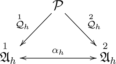I will say that two strict quantizations ${({\stackrel{1}{𝔄}}_h,{\stackrel{1}{𝒬}}_h)}_{h\in [0,1]}$ and ${({\stackrel{2}{𝔄}}_h,{\stackrel{2}{𝒬}}_h)}_{h\in [0,1]}$ of 𝒫, {⋅, ⋅} are equivalent just in case for each $h\in [0,1]$, there is an *-isomorphism ${\alpha }_h:{\stackrel{1}{𝔄}}_h\to {\stackrel{2}{𝔄}}_h$ such that the diagram in figure 1 commutes.Footnote ⁶ Two strict quantizations are equivalent when the fibers 𝔄 over each point $h\in [0,1]$ are *-isomorphic, in a way that allows one to identify the continuous sections of each continuous field. If one believes *-isomorphic C*-algebras have the capacity to represent the same physical systems, then it follows that equivalent continuous quantizations have the capacity to represent the classical limits for the same systems.

Figure 1.

Later, I construct two strict quantizations with conceptually distinct motivations. One quantization allows us to interpret varying values of $\hslash$ as corresponding to different worlds with different physics—this is the interpretation I take Rosaler and others to balk at. The other quantization allows us to interpret varying values of $\hslash$ as representing the same physical world in different systems of units—this is the interpretation I hope to show can be used to explain classical behavior. However, I will demonstrate that the resulting two strict quantizations are equivalent, thus allowing us to transfer my preferred interpretation to the mathematical structure in any of its equivalent instantiations.

It is worth making two remarks concerning the status of my definition of equivalent quantizations. First, the significance of equivalence of quantizations relies on the substantive assumption stated above: that *-isomorphic C*-algebras have the capacity to represent the same physical systems. This view about the use of mathematical models, mathematical equivalences, and representational capacities has been expressed in general terms elsewhere (Feintzeig Reference Feintzeig2015; Weatherall Reference Weatherall2018; Fletcher Reference Fletcher2020). Although the stated claim is controversial, I will simply take it on as an assumption without further argument and set the issue aside for present purposes.Footnote ⁷ One can understand my conclusions that rely on this assumption to be conditional on its acceptance. Yet, I also hope the spoils of this investigation provide some reason for making the assumption in the first place.

Second, my main conclusion that one can use the classical limit to explain classical behavior from quantum mechanics does not rely on the aforementioned assumption about the connection between equivalence and representational capacities. To establish this conclusion, I only need to show that there is some continuous quantization that can be given an interpretation suitable for the explanation of classical behavior. I believe this can be done using only the second continuous quantization I define below, which I call the “factual limit.” I believe it is illustrative to show that my preferred quantization is equivalent to a more standard formulation of the classical limit, whose interpretation has been deemed problematic. The mathematical equivalence I will demonstrate between these two quantizations is meant to aid our understanding of the new interpretation I provide. However, the equivalence is not necessary for my argument that one can give a partial explanation of classical behavior, and so for the main thesis of the article one need not accept the (perhaps controversial) assumption about isomorphisms and representational capacities that motivates my definition of equivalent quantizations.

3.2. Example: The Weyl Algebra

I now define a particular C*-algebra, known as the Weyl algebra that is often used to represent certain quantum systems (see Petz Reference Petz1990; Clifton and Halvorson Reference Clifton and Halvorson2001).Footnote ⁸ I will use this example to illustrate the concept of a strict deformation quantization. I will then draw on this example in section 4 when interpreting the classical limit with a precise notion of “approximation on certain scales.”

Start with a classical theory of a system with finitely many degrees of freedom and phase space given by ℝ²ⁿ. Such a system might consist of a finite number n of particles, each moving in one dimension. Each point $x=(q_1,\dots ,q_n,p_1,\dots ,p_n)\in {ℝ}^{2n}$, understood in some canonical coordinate system, lists the position q_j and momentum p_j of each of the n particles.

Physical magnitudes of this system can be represented as complex-valued functions on phase space $f:{ℝ}^{2n}\to ℂ$. Consider the family of functions $W_0\left(x\right):{ℝ}^{2n}\to ℂ$ for each $x\in {ℝ}^{2n}$ defined by

(2) $\begin{array}{}& W_0\left(x\right)\left(y\right)≔e^{\mathrm{ix}\cdot y},\end{array}$

where ⋅ is the standard inner product on ℝ²ⁿ. The classical Weyl algebra, denoted 𝒲₀, is defined as the C*-algebra containing all norm limits of polynomials of functions of the form W ₀(x) for $x\in {ℝ}^{2n}$, endowed with the algebraic structure of point-wise addition, multiplication, and complex conjugation and with the standard supremum norm.Footnote ⁹

One constructs the quantum Weyl algebra by starting from the same generating magnitudes W ₀(x) and deforming the commutative point-wise multiplication relation to obtain a noncommutative algebra. I denote by W_h(x) the element W ₀(x) understood now as an element of the quantum Weyl algebra. Define the noncommutative product on the quantum Weyl algebra by

(3) $\begin{array}{}& W_h\left(x\right)W_h\left(y\right)≔e^{\frac{\mathrm{ih}}{2}\sigma (x,y)}{W}_h(x+y)\end{array}$

for all x, $y\in {ℝ}^{2n}$. Here σ is the standard symplectic form on ℝ²ⁿ:

(4) $\begin{array}{}& \sigma \left(\right(q,p),(q^{\prime },p^{\prime }\left)\right)≔q^{\prime }\cdot p-q\cdot p^{\prime }\end{array}$

for q, p, q′, $p^{\prime }\in {ℝ}^n$, where ⋅ in the above expression is now the standard inner product on ℝⁿ. The quantum Weyl algebra 𝒲_h is the C*-algebra obtained as the completion of the collection of all polynomials (now with respect to the noncommutative multiplication operation) of magnitudes of the form W_h(x) for $x\in {ℝ}^{2n}$ in the so-called minimal regular norm (Manuceau et al. Reference Manuceau, Sirugue, Testard and Verbeure1974; Binz et al. Reference Binz, Honegger and Rieckers2004a, Reference Binz, Honegger and Rieckers2004b). The relation in equation (3) is known as the Weyl form of the canonical commutation relations because when the generators take their intended forms

(5) $\begin{array}{}& W_h(a,b)\sim e^{i(a\cdot Q+b\cdot P)}\end{array}$

for the quantum position operator Q and momentum operator P (as in the Schrödinger representation), equation (3) is equivalent to the familiar relation

(6) $\begin{array}{}& [Q,P]=i\hslash \text{.}\end{array}$

One can use these algebraic tools to construct a strict deformation quantization, which can be used to represent the classical limit of the quantum systems represented by the Weyl algebra. Binz et al. (Reference Binz, Honegger and Rieckers2004b) show that there is a Poisson algebra (𝒫, {⋅, ⋅}), norm dense in 𝒲₀, containing all “suitably smooth” magnitudes. Here, {⋅, ⋅} is just the usual Poisson bracket determined by the standard symplectic form σ. The quantization maps ${𝒬}_h:𝒫\to {𝒲}_h$ for each $h\in [0,1]$ are defined as the linear extension of

(7) $\begin{array}{}& {𝒬}_h\left(W_0\right(x\left)\right)≔W_h\left(x\right)\end{array}$

for all $x\in {ℝ}^{2n}$. With the quantization maps so defined, the family ${({𝒲}_h,{𝒬}_h)}_{h\in [0,1]}$ is a strict deformation quantization. Furthermore, one can define a collection of continuous sections 𝒦 as the smallest C*-subalgebra of ${\prod }_{h\in [0,1]}{𝔄}_h$ containing the maps [ $h\mapsto {𝒬}_h\left(A\right)$] for each $A\in 𝒫$. Then with the global quantization map $𝒬:𝒫\to 𝒦$ defined by

$𝒬\left(A\right)\left(h\right)≔{𝒬}_h\left(A\right)$

for all $A\in 𝒫$, the structure ( ${\left({𝒲}_h\right)}_{h\in [0,1]}$, 𝒦, 𝒬) becomes a continuous quantization. Thus, one can encode the classical limit of a quantum system represented by the Weyl algebra in a continuous field of C*-algebras. I spell out in more detail in section 4 how one can interpret the mathematical structure specified by this continuous field of algebras as I use this example to illustrate the notion of “approximation on certain scales” at play in the classical limit.

4. A Notion of Approximation

Now that we have some familiarity with continuous quantizations, it is the purpose of this section to interpret the mathematical tools they provide. Specifically, in this section I argue that continuous quantizations provide tools for interpreting the classical limit of quantum theories through a notion of “approximation on certain scales.” I argue that the spectral theorem, which already plays a central role in the interpretation of quantum theories, is also essential to this notion of approximation.

4.1. The Spectral Theorem and Numerical Values

The main idea of my interpretation of continuous quantizations is that a quantization map can be interpreted as identifying operators that represent the same physical quantity in different systems of units. This interpretation is possible because we can identify projection operators as providing theoretical content that is independent of a system of units, and the spectral theorem shows how general quantities are related to projections. My first task in the current section is to make this interpretation of projections and the spectral theorem precise before proceeding to their interplay with quantization maps.

To begin, recall that, while a general self-adjoint operator $A\in 𝔄$ can be used to represent a real-valued physical magnitude, one can say more about the representational capacities of a projection E. Projections are capable of representing propositions. Since $\mathrm{sp}\left(E\right)=\{0,1\}$, one can think of the two possible values of E as true (1) and false (0). The usual rules for calculating the expectation value of a projection give the probability that the proposition represented by E is true (a number in [0, 1]), which agrees with the Born rule for calculating the probabilities of outcomes for magnitudes represented by self-adjoint operators (see also Scheibe Reference Scheibe1973, chaps. 2–3).

I claim that one can interpret general self-adjoint operators as differing from projections in the following sense: while the values of the physical magnitudes represented by general self-adjoint operators almost always vary in different systems of units, the values of a proposition represented by a projection stay the same. Suppose, for example, that A is a self-adjoint operator representing a position magnitude for a particle.Footnote ¹⁰ Then changing units of distance from m to cm changes the possible values the magnitude represented by A can take on, scaling the numerical values by 100 (e.g., $4 \text{m}\mapsto 400 \text{cm}$). But, suppose E_O is a projection representing the proposition “the particle is located in the region represented by O.” If the particle is located in the region represented by O, then the proposition represented by E_O is true and takes the value 1, whereas if the particle is outside of the region represented by O, then the proposition represented by E_O is false and takes the value 0. These values are unitless: the particle is either in the region represented by O or not, regardless of whether we refer to O in units of m or cm.

On this interpretation, it follows that while one can hold fixed the projection operator used to represent a given proposition, one may need to use different self-adjoint operators to represent the same physical magnitude in different systems of units. In the previous example, while we can use E_O to represent the given proposition in any system of units, if we use A to represent the position magnitude in units of m, then we will need to use some other operator, whose numerical values are scaled by 100, to represent the same position magnitude in units of cm. The spectral theorem informs us as to which self-adjoint operator we should use to represent the same physical magnitude in a different system of units.

Recall that the spectral theorem (see Reed and Simon Reference Reed and Simon1980, chap. 7; Kadison and Ringrose Reference Kadison and Ringrose1997, sec. 5.2) states that for every physical magnitude represented by a self-adjoint element A of a C*-algebra 𝔄, there is a projection valued measure $E:B\left(\mathrm{sp}\right(A\left)\right)\to {𝔄}^{\ast \ast }$ such that

(8) $\begin{array}{}& A={\int }_{\mathrm{sp}\left(A\right)}\lambda {\mathrm{dE}}_{\lambda },\end{array}$

where λ is understood as the identity function on sp(A). Here, B(sp(A)) is the Borel σ-algebra of sp(A), and E takes values in the universal enveloping W*-algebra 𝔄** of 𝔄.

The spectral theorem tells us we can understand physical magnitudes as assigning numerical values to associated propositions. For example, the position magnitude expressed in units of m assigns to the proposition “the particle is 4 m from the origin” the numerical value 4. The numerical values that a magnitude assigns to each proposition are fixed by the association of the projections with values $\lambda \in \mathrm{sp}\left(A\right)$ (or really a range of values for λ in a Borel subset). The spectral theorem tells us that this information—a collection of projections and an association of them with numerical values—is sufficient to reconstruct the original self-adjoint operator representing the physical magnitude in the given system of units.

The spectral theorem also informs us about which operator we should use to represent the same physical magnitude in a different system of units. Generally, a physical magnitude expressed in different systems of units will associate the same propositions with different numerical values. For example, if one changes units from m to cm, the position magnitude then assigns to the very same proposition “the particle is 4 m from the origin” the new numerical value 400. This is because the projection also represents the (identical) proposition “the particle is 400 cm from the origin.”

This is all the information we need to figure out which operator we should use to represent the same physical magnitude in a new choice of units because it tells us to replace the identity function λ in the integral expression of equation (8) with a different Borel function $f:\mathrm{sp}\left(A\right)\to ℂ$. For example, in the unit change from m to cm, the function f is $f\left(\lambda \right)=100\lambda$ for all $\lambda \in \mathrm{sp}\left(A\right)$. This new function f associated with the unit change can be thought of as either reassigning the physical magnitude new numerical values by rescaling them or equivalently reassociating the spectral projections E _λ with new numerical values f(λ).

Knowing the new numerical values we want to associate with a physical magnitude, we now know that we should use the operator

(9) $\begin{array}{}& A^{\prime }≔{\int }_{\mathrm{sp}\left(A\right)}f\left(\lambda \right){\mathrm{dE}}_{\lambda }\end{array}$

to represent the same physical magnitude we previously used A to represent, now considered in the new system of units. To summarize, the interpretation I am advocating entails that we can use the operators A and $A^{\prime }=f\left(A\right)$ to represent the same physical magnitude in different systems of units. In our example, while we use the operator A to represent the position magnitude in units of m, we should now use $A^{\prime }=f\left(A\right)=100A$ to represent the position magnitude in units of cm. Heuristically, we might say that the unit change induces a “transformation” $A\mapsto f\left(A\right)$. All we mean by this, though, is that we should in general use a different operator to represent the same physical magnitude when we work in a different system of units.

The reason the foregoing is important is that a quantization map provides us with precisely the tools we need to explicitly identify which elements of an algebra represent the same physical magnitude. In particular, if $A\in {𝔄}_0$ represents a physical magnitude in a classical theory, then we will understand 𝒬_h(A) to represent the same physical magnitude in a quantum theory in units in which Planck’s constant takes on the numerical value h. Reflecting on unit changes helps us see the relationship between 𝒬_h(A) and 𝒬_h′(A) for different numerical values h, h′ of Planck’s constant. In other words, we will see that one can express 𝒬_h′(A) as f(𝒬_h(A)) for a function $f:\mathrm{sp}\left({𝒬}_h\right(A\left)\right)\to ℂ$ specifying a change of units.

In the next subsection, I make the preceding remarks about quantization maps precise using the interpretation outlined in this section. Note, however, that I am not claiming that the interpretation just offered of the relationship between self-adjoint operators and projections is the only one available. An alternative interpretation in which projections “transform” under unit changes may also be possible, but I will not consider it here. I have offered one coherent and precise interpretation that will be helpful as we proceed; I claim only that one can take this interpretation but not that one is forced to. This is sufficient for my goal, which is only to show that it is possible to give an interpretation in which the classical limit can be used to explain the success of classical physics.

4.2. Units, Scales, and (Counter)factual Limits

When interpreting limits of physical constants like $\hslash \to 0$, there are two different approaches one can take. Following Fletcher (Reference Fletcher2019) (who draws on Rohrlich Reference Rohrlich1989), I will call these the counterfactual and factual approaches to interpreting the classical limit.Footnote ¹¹

Just as Gamow’s Mr. Tompkins dreams of a world in which macroscopic objects like billiard balls display the strangeness of the quantum world (Gamow Reference Gamow1993, chap. 7), the counterfactual approach attempts to answer the question, “How would the world be different if Planck’s constant $\hslash$ were to take a different value?” The counterfactual interpretation appears to answer questions only about other possibilities apart from the actual world. But, the factual approach attempts to answer the question, “In the actual world, how do quantities behave in different systems of units in which Planck’s constant $\hslash$ takes different values?” Thus, the two approaches differ on whether they are concerned with modeling the actual world with the actual observations and experiments (factual interpretation) or alternative physical possibilities (counterfactual interpretation).

It seems that only the factual interpretation can answer explanatory questions about approximate classical behavior in our world. So if one thought current mathematical resources required a counterfactual interpretation, there would appear to be a conceptual gap. And indeed, the passages quoted in section 2 suggest that Nickles, Radder, and Rosaler have something like a counterfactual interpretation in mind when they object to the explanatory power of the $\hslash \to 0$ limit. In what follows, I establish the viability and the significance of a factual interpretation of the $\hslash \to 0$ limit. I take this factual interpretation to provide a response to the preceding worries and also to make precise the sense in which the $\hslash \to 0$ limit explains the theoretical structure of classical mechanics. I begin by clarifying the counterfactual interpretation so that we can use it for comparison.

4.2.1. Counterfactual Quantization

It is not hard to see how one would give a counterfactual interpretation of the continuous quantization of the Weyl algebra specified at the end of section 3. On this interpretation, one represents a different “world” for each value of $\hslash$ by taking the physical quantities of the system to form a distinct algebra ${\stackrel{\mathrm{CF}}{𝔄}}_h={𝒲}_h$. One can keep fixed the classical “world” in which quantities are represented by elements of ${\stackrel{\mathrm{CF}}{𝔄}}_0={𝒲}_0$. The counterfactual quantization map ${\stackrel{\mathrm{CF}}{𝒬}}_h={𝒬}_h$ defined in equation (7) then identifies the “same” or “counterpart” magnitudes in distinct worlds.

This indeed defines a strict and continuous deformation quantization (with counterfactual continuous sections $\stackrel{\mathrm{CF}}{𝒦}=𝒦$), as discussed previously. And the apparatus so defined matches the intuition of the counterfactual approach that each “world” can be interpreted as being governed by distinct laws because each world realizes a different commutation relation:

(10) $\begin{array}{}& W_h\left(x\right)W_h\left(y\right)=e^{\frac{\mathrm{ih}}{2}\sigma (x,y)}{W}_h(x+y)\end{array}$

for all x, $y\in {ℝ}^{2n}$. Thus, one can understand the “worlds” represented by the counterfactual quantization to really be physically different. I think it is understandable that other authors would balk at such a structure as useful for giving explanations in our own world. I agree with the insinuations of Nickles, Radder, and Rosaler quoted in section 2: the significance of the counterfactual interpretation is opaque.

I will not attempt to show that facts about other possible worlds can be used to explain facts about the actual world. Instead, I believe it is worthwhile to develop an alternative factual interpretation. I will do so in the remainder of this section by defining an alternative strict quantization that encodes varying values of $\hslash$ as representing the same world in different systems of units. I will establish that this structure indeed forms a strict and continuous deformation quantization by showing it is equivalent to the counterfactual quantization. If one accepts my interpretation of equivalence from section 3, then it follows that one could just as well give a factual interpretation of the counterfactual quantization structure. But even if one rejects my interpretation of equivalence, I will still have shown that a factual interpretation of the $\hslash \to 0$ limit is possible, and it is this interpretation that I take to be explanatory.

4.2.2. Factual Quantization

On the factual approach, one wants to specify algebras ${\stackrel{F}{𝔄}}_h$ that represent physical quantities in the actual world and use the index h only to investigate how these quantities change in different systems of units. Since one wants to model quantities in only the actual world, one can start with the constraint that all of the algebras ${\stackrel{F}{𝔄}}_h$ be identical. So let us fix our world in units where $h=1$ and define ${\stackrel{F}{𝔄}}_h≔{𝒲}_1$ for all $h\in (0,1]$. Of course, since one wants to explain classical behavior, one still needs to let ${\stackrel{F}{𝔄}}_0≔{𝒲}_0$. One then uses a quantization map to identify how each physical quantity changes in the actual world when one changes units so that the numerical value of Planck’s constant changes as $h^{\prime }\mapsto h$ (for arbitrary h, $h^{\prime }\in (0,1]$). In other words, we will proceed to define ${\stackrel{F}{𝒬}}_h$ so that for each $A\in 𝒫$, 𝒬_h(A) represents the same physical magnitude as A in the quantum theory expressed in a system of units in which Planck’s constant $\hslash$ takes the numerical value h.

To think about these changes of units, let us start by analyzing the classical quantities. It will be helpful to specify a canonical coordinate system (q ₁, …, q_n, p ₁, …, p_n) on the classical phase space ℝ²ⁿ and expand the operators W ₀(x), where $x=(a_1,\dots ,a_n, b_1,\dots ,b_n)$:

(11) $\begin{array}{}& W_0(a_1,\dots ,a_n, b_1,\dots ,b_n)(q_1,\dots ,q_n, p_1,\dots ,p_n)=e^{i(a_1{q}_1+\dots +a_n{q}_n+b_1{p}_1+\dots +b_n{p}_n)}\text{.}\end{array}$

For concreteness, suppose that the unit change that induces the change in the numerical value of Planck’s constant $h^{\prime }\mapsto h$ is a change of distance units (e.g., cm to m).Footnote ¹² To understand how this affects the numerical values of quantities involved, recall that Planck’s constant has units ( $(\mathrm{mass}\cdot {\mathrm{distance}}^2)/\mathrm{time}$), each position quantity q_j has units (distance), and each momentum quantity p_j has units ( $(\mathrm{mass}\cdot \mathrm{distance})/\mathrm{time}$). Since Planck’s constant involves units of distance², while position and momentum involve units only of distance, if one changes units of distance in a way that induces a change in numerical values $h^{\prime }\mapsto h$, this will change the numerical values of position and momentum by

(*) $\begin{array}{}& \begin{array}{cc}{q}_j\mapsto \sqrt{\frac{h}{h^{\prime }}}& \cdot q_j\\ p_j\mapsto \sqrt{\frac{h}{h^{\prime }}}& \cdot p_j\text{.}\end{array}\end{array}$

Now, let us shift focus to the magnitudes W ₁(a ₁, …, a_n, b ₁, …, b_n) for the corresponding quantum system. In this case, if one restricts attention to the (regular) Schrödinger representation (π, L ²(ℝⁿ)) of the Weyl algebra,Footnote ¹³ then the Weyl unitaries take the following form (cf. eq. [5]):

(12) $\begin{array}{}& \pi \left(W_1\right(a_1,\dots ,a_n, b_1,\dots ,b_n\left)\right)=e^{i(a_1{Q}_1+\dots +a_n{Q}_n+b_1{P}_1+\dots +b_n{P}_n)}\end{array}$

for self-adjoint unbounded operators Q ₁, …, Q_n, P ₁, …, P_n representing the quantized position and momentum magnitudes. Although generally Q_j and P_j will not belong to any C*-algebra ${\stackrel{F}{𝔄}}_h$ because they are unbounded, one may restrict attention to the Schrödinger representation in which the spectral theorem still applies.

So suppose Q_j is a position magnitude affiliated with the quantum system. Let E denote the projection valued measure in the Schrödinger representation associated with Q_j:

(13) $\begin{array}{}& Q_j={\int }_{\mathrm{sp}\left(Q_j\right)}\lambda {\mathrm{dE}}_{\lambda }\text{.}\end{array}$

On the interpretation of projections and self-adjoint operators outlined above, a unit change that induces the change in numerical values of Planck’s constant $h^{\prime }\mapsto h$ leaves each projection E fixed but changes the values that Q_j associates to E according to the scale factor $\sqrt{h/h^{\prime }}$ as per equation (*). This yields a change

(14) $\begin{array}{}& Q_j\mapsto Q_j^{\prime }={\int }_{\mathrm{sp}\left(Q_j\right)}\sqrt{\frac{h}{h^{\prime }}}\cdot \lambda {\mathrm{dE}}_{\lambda }=\sqrt{\frac{h}{h^{\prime }}}\cdot Q_j\text{.}\end{array}$

Similarly, suppose P_j is a momentum magnitude affiliated with the quantum system, understood as the standard momentum operator in the Schrödinger representation of the Weyl algebra associated with projection valued measure F:

(15) $\begin{array}{}& P_j={\int }_{\mathrm{sp}\left(P_j\right)}\lambda {\mathrm{dF}}_{\lambda }\text{.}\end{array}$

Again, a change of units that induces the change in numerical values of Planck’s constant $h^{\prime }\mapsto h$ leaves each projection F fixed but changes the values that P_j associates to F according to the scale factor $\sqrt{h/h^{\prime }}$ as per equation (*). This yields a change

(16) $\begin{array}{}& P_j\mapsto P_j^{\prime }={\int }_{\mathrm{sp}\left(P_j\right)}\sqrt{\frac{h}{h^{\prime }}}\cdot \lambda {\mathrm{dF}}_{\lambda }=\sqrt{\frac{h}{h^{\prime }}}\cdot P_j\text{.}\end{array}$

Now, let us use this change of units to define the factual quantization map ${\stackrel{F}{𝒬}}_h:𝒫\to {\stackrel{F}{𝔄}}_h$. First, we can simplify our expressions by recalling that we wish to model changing units from ${\stackrel{F}{𝔄}}_{h^{\prime }}={𝒲}_1$ in which the numerical value of Planck’s constant is $\hslash =h^{\prime }=1$. So this unit change induces the change in numerical values $1\mapsto h$ with scaling factor $\sqrt{h/h^{\prime }}=\sqrt{h}$. This motivates defining the factual quantization map as the linear continuous extension of

(17) $\begin{array}{}& {\stackrel{F}{𝒬}}_h\left(W_0\right(a_1,\dots ,a_n, b_1,\dots ,b_n\left)\right)≔W_1(\sqrt{h}\cdot a_1,\dots ,\sqrt{h}\cdot a_n, \sqrt{h}\cdot b_1,\dots ,\sqrt{h}\cdot b_n)\end{array}$

for all $(a_1,\dots ,a_n, b_1,\dots ,b_n)\in {ℝ}^{2n}$. This appears in the Schrödinger representation as

(18) $\begin{array}{}& \pi \left(W_1\right(\sqrt{h}\cdot a_1,\dots ,\sqrt{h}\cdot a_n, \sqrt{h}\cdot b_1,\dots ,\sqrt{h}\cdot b_n\left)\right)=e^{i(a_1\sqrt{h}\cdot Q_1+\dots +a_n\sqrt{h}\cdot Q_n+b_1\sqrt{h}\cdot P_1+\dots +b_n\sqrt{h}\cdot P_n)}\end{array}$

with each Q_j and P_j scaled by the factor $\sqrt{h}$ as desired. More succinctly, one can write

(19) $\begin{array}{}& {\stackrel{F}{𝒬}}_h\left(W_0\right(x\left)\right)=W_1(\sqrt{h}\cdot x)\end{array}$

for all $x\in {ℝ}^{2n}$.

Notice that the operators W ₁(x) for $x\in {ℝ}^{2n}$ obey the standard commutation relation

(20) $\begin{array}{}& W_1\left(x\right)W_1\left(y\right)=e^{\frac{i}{2}\sigma (x,y)}{W}_1(x+y)\end{array}$

for all x, $y\in {ℝ}^{2n}$. This relation remains fixed in each of the algebras ${\stackrel{F}{𝔄}}_h={𝒲}_1$, indicating that the physical laws remain the same in the one “world” we represent.

With this factual quantization map, one can follow the procedure of section 3.2 to construct a continuous quantization ( ${\left({\stackrel{F}{𝔄}}_h\right)}_{h\in [0,1]}$, $\stackrel{F}{𝒦}$, $\stackrel{F}{𝒬}$). Define the collection of factual continuous sections $\stackrel{F}{𝒦}$ as the smallest C*-subalgebra of ${\prod }_{h\in [0,1]}{\stackrel{F}{𝔄}}_h$ containing the maps [ $h\mapsto {\stackrel{F}{𝒬}}_h\left(A\right)$] for all $A\in 𝒫$. Define the factual global quantization map $\stackrel{F}{𝒬}:𝒫\to \stackrel{F}{𝒦}$ by

$\stackrel{F}{𝒬}\left(A\right)\left(h\right)≔{\stackrel{F}{𝒬}}_h\left(A\right)\mathrm{.}$

This structure provides a continuous quantization of 𝒫, as I establish next by showing it is equivalent to the counterfactual quantization.Footnote ¹⁴

4.2.3. Factual Interpretation

Now that we have constructed two mathematical structures with quite different motivations—the counterfactual quantization for alternative possible worlds and the factual quantization for our world—I will establish that both mathematical structures have the same representational capacities. That is, I will show that the counterfactual ( ${\left({\stackrel{\mathrm{CF}}{𝔄}}_h\right)}_{h\in [0,1]}$, $\stackrel{\mathrm{CF}}{𝒦}$, $\stackrel{\mathrm{CF}}{𝒬}$) and the factual ( ${\left({\stackrel{F}{𝔄}}_h\right)}_{h\in (0,1]}$, $\stackrel{F}{𝒦}$, $\stackrel{F}{𝒬}$) continuous quantizations are equivalent.

For each $h\in (0,1]$, define ${\alpha }_h:{\stackrel{\mathrm{CF}}{𝔄}}_h\mapsto {\stackrel{F}{𝔄}}_h$ as the unique linear, norm continuous extension ofFootnote ¹⁵

(21) $\begin{array}{}& {\alpha }_h\left(W_h\right(x\left)\right)≔W_1(\sqrt{h}\cdot x)\mathrm{.}\end{array}$

It suffices to notice that

(22) $\begin{array}{}& W_1(\sqrt{h}\cdot x)\cdot W_1(\sqrt{h}\cdot y)=e^{\frac{\mathrm{ih}}{2}\sigma (x,y)}{W}_1\left(\sqrt{h}\right(x+y\left)\right)\end{array}$

for all x, $y\in {ℝ}^{2n}$ due to the fact that $\sigma (\sqrt{h}\cdot x, \sqrt{h}\cdot y)=h\cdot \sigma (x,y)$. This establishes that α_h is an *-isomorphism for each $h\in (0,1]$ and, by construction,

(23) $\begin{array}{}& {\alpha }_h\circ \stackrel{\mathrm{CF}}{{𝒬}_h}=\stackrel{F}{{𝒬}_h}\mathrm{.}\end{array}$

Hence, the two quantizations are equivalent.

This establishes that the factual quantization defined above is indeed a continuous quantization. Furthermore, this shows that even the counterfactual quantization (i.e., the quantization presented in sec. 4.2.1) can be interpreted as showing that classical kinematics holds in our world “approximately on certain scales.” That is, one can import the notion of “approximation on certain scales” from the factual quantization to either of these mathematical structures. So what is the notion of “approximation on certain scales” in the factual quantization?

In the factual continuous quantization, suppose we are given arbitrary classical quantities A, $B\in 𝒫$ and a chosen numerical error bound $\epsilon >0$. It now follows from equation (1), repeated below for emphasis, that there is a choice of units (i.e., some combination of distance, time, and mass units) in which Planck’s constant $\hslash$ takes on a numerical value h such that in this system of units the behavior of 𝒬_h(A) and 𝒬_h(B) is “within ε” of the behavior of A and B:

(24) $\begin{array}{}& \begin{array}{cc}\left|{\Vert {𝒬}_h\left(A\right)\Vert }_h-{\Vert A\Vert }_0\right|& <\epsilon \\ {\Vert {𝒬}_h\left(A\right){𝒬}_h\left(B\right)-{𝒬}_h\left(\mathrm{AB}\right)\Vert }_h& <\epsilon \\ {\Vert \left[{𝒬}_h\right(A),{𝒬}_h(B\left)\right]-{𝒬}_h\left(\right\{A,B\left\}\right)\Vert }_h& <\epsilon \mathrm{.}\end{array}\end{array}$

Similarly, for every $h^{\prime }<h$, the inequalities (24) will hold with h replaced by h′. Notice further that this implies that for any state ω on 𝔄_h,

(25) $\begin{array}{}& \begin{array}{cc}\left|\omega \left({𝒬}_h\right(A\left){𝒬}_h\right(B\left)\right)-\omega \left({𝒬}_h\right(\mathrm{AB}\left)\right)\right|& <\epsilon \\ \left|\omega \left(\right[{𝒬}_h\left(A\right),{𝒬}_h\left(B\right)\left]\right)-\omega \left({𝒬}_h\right(\{A,B\}\left)\right)\right|& <\epsilon ,\end{array}\end{array}$

and so the expectation values of relevant physical quantities are within ε of one another. Thus, 𝒬_h(A) and 𝒬_h(B) approximate A and B at all “scales” above the one defined by the value of the error bound ε and the system of units in which Planck’s constant $\hslash$ takes the numerical value h.

The notion of “scale” here has a particular precise meaning. It corresponds to the physical size of the interval that the number ε determines. The very same numerical error bound ε determines a physically larger or smaller interval as we change units. This is because the same number, when viewed in different systems of units, may represent a larger or smaller physical quantity. It follows from the inequalities in equation (25) that even when the numerical (expectation) values of the physical magnitudes 𝒬_h(A)𝒬_h(B) and 𝒬_h(AB) differ wildly in one choice of units, they will be close together in another. Thus, we recover the intuitive notion that as $\hslash \to 0$, we “zoom out” from the quantum system by caring less and less about the microscopic details. The way one coarse-grains from the microscopic details is by fixing a numerical error bound ε and changing units so that ε represents a physically larger interval of allowable error. The typical interpretation is that experiments probe the system on larger “scales” because qualitative precision decreases as allowable error increases.

Notice that the spectral theorem plays a crucial role in this interpretation. In order to understand the $\hslash \to 0$ limit under this notion of “approximation at certain scales,” one understands a change in the numerical value h to correspond to a change of units. This can be accomplished precisely because one has spectral projections for each physical magnitude, which are held fixed even as units change. Thus, the spectral projections and the relations among them represent the “invariant” (under unit changes) physical content of the theory.

It is worth stressing that on the current interpretation, a choice of units on its own does not define a scale. Instead, a scale is determined by both the numerical value of the error bound ε and the units in which it is expressed. This means that a scale is not set by the system being measured but rather by the measurement procedure one uses to probe the system. One might object that this is not the notion of “scale” used colloquially in the physics community. I do not claim that this is the only notion of scale used by physicists, but I do believe it is one that has been employed to understand the classical limit (e.g., see Emch Reference Emch1983, 418), and I believe this notion of scale helps make precise a way of understanding the classical limit that is conceptually significant.Footnote ¹⁶ I am optimistic that this notion of scale is analogous to, or helpful for, making sense of scales and coarse-graining in other contexts like renormalization theory because it seems that particle physicists often have something like this notion of scale in mind.Footnote ¹⁷ My optimism may be unfounded, but I believe the interpretation just given is important in its own right regardless of future applications.

One might still worry about the notion of approximation I have just laid out. We are never in the position of specifying our tolerable error as a unitless number ε; the error tolerated by a measuring apparatus is typically specified in the units in which our apparatus displays measured values. But the analysis just given can be adapted immediately to this situation, as follows. To fix the units in which the error bound is expressed, one first needs to fix $\epsilon >0$ (say, fix $\epsilon =1$). The facts captured in equations (24) and (25) tell us that there is some system of units in which $\hslash$ takes the value $h\in (0,1]$, and in this system of units the number ε provides a tolerable bound. Now, comparing one’s preferred choice of units (e.g., natural units with $\hslash =1$) to the choice of units that yields the value h for Planck’s constant provides a way of converting the error ε from the system of units defined by $\hslash =h$ to the system of units defined by $\hslash =1$. The necessary unit change here will depend on the physical dimensions of the magnitudes considered, which align with the dimensions of ε. The important result is that if we fix a system of units, there exists an error bound (the number ε, reexpressed in preferred units) such that the difference of values of the relevant physical quantities lies within that error bound.

This notion of approximation is both weaker and stronger than one might like. It is weaker because one cannot arbitrarily choose both the error bound ε and the units in which it is expressed. If one fixes the number ε, then we know there exists a system of units for ε in which the approximation in equations (24) and (25) holds, but this may not agree with the units we prefer. Yet, if one fixes a system of units, then the value of the error bound will be determined by the existence of the unit transformation to be applied to ε, which again may not yield the error bound we prefer. This makes sense because classical and quantum mechanics make different predictions; one cannot be expected to make them coincide unless one is willing to lose precision in measurements.

But, the notion of approximation is also quite strong. For given physical magnitudes, the number ε provides a uniform bound on the tolerable error for expectation values of the magnitudes in all states. This is important because if one only considered one state at a time, it would be no surprise that one could make quantum expectation values close to classical expectation values by accepting a large enough error. What is surprising and significant is that there is a single notion of closeness, or a single error bound, that makes the expectation values of all states close enough.Footnote ¹⁸ This is what allows us to interpret the approximation as explaining the theoretical structure of classical mechanics. The uniform approximation of the norm and product explains the spectral properties of each magnitude (i.e., why it has a certain range of possible values). The uniform approximation of Poisson brackets by commutators explains why magnitudes have certain theoretical relations to each other that are encoded in the geometry of the classical phase space. It is the approximation of theoretical properties and relations of kinematic quantities that allows us to explain the theoretical structure of classical mechanics from quantum mechanics.

5. Discussion

I have now shown a sense in which the classical limit, when given a factual interpretation, can be used to explain the theoretical structure of classical mechanics from quantum mechanics. This explanation proceeds by establishing that in our world, the properties and relations of quantum magnitudes are “close” to the properties and relations of classical magnitudes. Here, “close” means that there is a uniform error bound for the difference between the predictions given by the quantum and classical expectation values; this error bound is uniform in the sense that it provides a single bound for all possible states. Mathematically, this error bound is encoded in a numerical value ε and a choice of units specified by the numerical value of Planck’s constant. It is the choice of units that varies as $\hslash \to 0$ and together with the number ε determines a “scale” for probing the system.

My analysis here agrees with Rosaler (Reference Rosaler2015a) that empirical information is needed to determine the appropriate error bound for a given situation or experiment.Footnote ¹⁹ The classical limit does not guarantee that use of classical mechanics will suffice for arbitrary levels of precision, and so it may not suffice for a given empirical situation. But, the classical limit entails the existence of some level of precision on which one can apply the structure of classical mechanics, if one allows for a large enough error bound.

My analysis differs from Rosaler’s in that I only explain the kinematic structure of classical mechanics. I have completely ignored dynamics, which is Rosaler’s central concern and perhaps the reason he approaches the problem through decoherence theory. This difference is not a disagreement; it shows that our concerns are orthogonal in one respect. I believe results from Landsman (Reference Landsman1998, Sec. II.2.7) may serve to extend the interpretation offered here to dynamical structure. But I also believe the treatment of dynamics and decoherence Rosaler offers is important and complementary to my approach.

My position differs from Rosaler’s in a further substantive way. Rosaler only explains the success of the empirical predictions of classical mechanics, while I claim that one can go further and explain its theoretical structure. In this way, I also disagree with Radder (Reference Radder1991), and I provide at least one example of a reductive explanation along the lines of what is advocated for by Post (Reference Post1971). Whereas Rosaler’s results are restricted to approximations for expectation values of individual states as in equation (25), I claim that the approximations captured by equation (24) are of central importance. Only these uniform approximations of products and commutators can serve to explain the spectral structure of classical quantities, which encodes their possible values, and their Poisson structure, which encodes their geometrical relations.Footnote ²⁰

Finally, I take my interpretation to be compatible with the common understanding of the $\hslash \to 0$ limit that treats the parameter $\hslash$ as a “dimensionless ratio.” Recall that this interpretation is advocated for by Batterman (Reference Batterman2002, 99 n. 1) and also by Landsman (Reference Landsman2017, 247). I believe the dimensionless ratio interpretation especially helps us understand the classical limits of quantum states (or continuous fields of states) because particular states can determine the values of quantities like temperature, length, or momentum that one needs to compare to $\hslash$ to construct the appropriate dimensionless ratio. My explanation of the kinematic structure of classical mechanics does not depend on such a choice of a continuous field of states. But this should not suggest that my dimensionful interpretation of the classical limit is in conflict with the dimensionless ratio interpretation.

On my view, it would be all the better if there were multiple ways of interpreting the mathematical structures used to model the classical limit. I only claim the interpretation given above in terms of “approximation on certain scales” is one possibility. This interpretation is useful for capturing the explanatory utility of the classical limit, although it may not be the only interpretation or the best one for all purposes. I have argued that the classical $\hslash \to 0$ limit, understood in terms of continuous fields of C*-algebras, gives rise to one way of explaining the success of the kinematic framework of classical mechanics; I believe this explanation deserves both recognition and philosophical attention.