1. Introduction
Beekeeping has steadily increased in importance in Africa and is widely promoted as an income diversification method because of its low start-up costs and production of valuable products such as honey and beeswax (Wagner et al., Reference Wagner, Meilby and Cross2019; Schouten, Reference Schouten2021; Nganso et al., Reference Nganso, Agboka, Atagong, Topé, Massing, Landmann, Sevgan, Mwiza, Odera, Piiru, Otieno-ayayo, Soroker and Guimapi2025). The benefits extend beyond direct income and include the ecosystem service of crop pollination. Globally, concerns have been raised regarding the decline of wild bees and other pollinators (Potts et al., Reference Potts, Biesmeijer, Kremen, Neumann, Schweiger and Kunin2010). The decline in pollinators, in turn, threatens the quality and quantity of crops (Klein et al., Reference Klein, Vaissière, Cane, Steffan-dewenter, Cunningham, Kremen and Tscharntke2007; Smith et al., Reference Smith, Singh, Mozaffarian and Myers2015; Bauer and Sue Wing, Reference Bauer and Sue Wing2016). Managed pollinators, such as honeybees, are a promising solution to stabilize yields and improve nutritional quality (Bommarco et al., Reference Bommarco, Marini and Vaissière2012; Khalifa et al., Reference Khalifa, Elshafiey, Shetaia, El-wahed, Algethami, Musharraf, AlAjmi, Zhao, Masry, Abdel-daim, Halabi, Kai, Al Naggar, Bishr, Diab and El-seedi2021). Beyond increasing yield, improving nutritional quality through pollination could help reduce nutrient gaps in low-income countries. In sub-Saharan Africa, pollinator-dependent (PD) crops have been shown to contribute the majority of essential micronutrients, potentially reducing nutrient deficiencies (Mulungu et al., Reference Mulungu, Tekelewold, Abro, Sevgan, Muriithi, Ecuru, Beesigamukama and Kassie2023).
The economics literature on the value of pollination services of managed bees has a long history, dating back to seminal works that framed it as a classic positive externality requiring policy intervention, such as subsidies, to ensure optimal provision (Meade, Reference Meade1952). This interest has surged following global evidence of pollinator decline (Potts et al., Reference Potts, Biesmeijer, Kremen, Neumann, Schweiger and Kunin2010). This led to the emergence of macro-level valuations that estimate the contribution of animal pollination to food production in the hundreds of billions of dollars annually (Gallai et al., Reference Gallai, Salles, Settele and Vaissière2009; Ramírez and Kallarackal, Reference Ramírez and Kallarackal2018). A rich strand of literature exists on pollination markets, particularly in the USA, exploring honeybee population dynamics, migratory beekeeping and the economics of pollination services (Rucker et al., Reference Rucker, Thurman and Burgett2012; Champetier et al., Reference Champetier, Sumner and Wilen2015).
Although several studies find a positive impact of beekeeping on income in Africa, the pollination benefits of this important economic activity are not rigorously quantified (Schouten, Reference Schouten2021; Abro et al., Reference Abro, Kassie, Tiku, Taye, Ayele and Ayalew2022). In addition, the existing evidence on yield and quality gains from pollination is limited to experimental studies (Khalifa et al., Reference Khalifa, Elshafiey, Shetaia, El-wahed, Algethami, Musharraf, AlAjmi, Zhao, Masry, Abdel-daim, Halabi, Kai, Al Naggar, Bishr, Diab and El-seedi2021). Existing research is overwhelmingly focused on high-income countries, with a notable absence of household-level quantitative studies assessing the economic impact of beekeeping and pollination externalities on crop production in low-income countries (Breeze et al., Reference Breeze, Gallai, Garibaldi and Li2016; Abro et al., Reference Abro, Kassie, Tiku, Taye, Ayele and Ayalew2022). Furthermore, the canonical issue of pollination externality in smallholder farming contexts has not been quantified, leaving an important policy variable unmeasured.
This study addresses these gaps by using the Living Standards Measurement Survey (LSMS) panel data from Ethiopia, a nationally representative dataset, to quantify the economic benefits of managed beekeeping at the farm level. The objectives of this study are threefold. First, we estimate the effect of beekeeping on crop revenue, accounting for any improvements in yield or output quality. Second, we estimate the effects of beekeeping's pure externality (social benefits) on the crop revenue of non-beekeepers and hence provide the first estimate of the social benefits of bees that are not accounted for in studies focusing only on beekeepers. Third, we disentangle the channels through which managed bees benefit crop production: whether by increasing crop yields or by improving crop quality (proxied by market prices). We find a significant positive impact of beekeeping on crop revenue, driven by mostly improved crop quality, with important positive externalities for non-beekeepers, underscoring a substantial, yet often uncounted, social return of beekeeping.
We provide a direct and rigorous estimate of the impact of managed bees on crop income, a topic that is currently scarcely covered and heavily skewed towards high-income countries (Breeze et al., Reference Breeze, Gallai, Garibaldi and Li2016). Complementing existing national or regional aggregate analyses and small-scale experimental trials, which often fail to capture large-scale, real farm conditions, our quantitative farm-level findings add a crucial pollination dimension to the well-recognized role of beekeeping as an income diversification strategy in Africa (Breeze et al., Reference Breeze, Gallai, Garibaldi and Li2016; Schouten et al., Reference Schouten2021; Abro et al., Reference Abro, Kassie, Tiku, Taye, Ayele and Ayalew2022). This evidence shows that the economic and ecological value of beekeeping extends beyond honey production, directly contributing to crop productivity and resilience at the farm level.
We also contribute to the long-standing research on the economic gains from pollination by going beyond simple yield-based assessment to quantify the price-mediated pathway. As Garratt et al. (Reference Garratt, Breeze, Jenner, Polce, Biesmeijer and Potts2014) stated, many studies have likely underestimated the value of pollination services by ignoring how quality improvements can lead to higher prices. Our work addresses this gap by capturing the full economic value of pollination, including the price premiums farmers receive for higher-quality produce because of bees pollination. We thus contribute to the very few studies that successfully disentangle the effect on crop yield from the effect on crop quality (Garratt et al., Reference Garratt, Breeze, Jenner, Polce, Biesmeijer and Potts2014). In the African context, where most development interventions view beekeeping mainly as a source of income diversification and livelihood improvement through honey and beeswax, our findings underscore the broader economic value of pollination services that extend beyond honey production. Recognizing pollination as a key driver of agricultural productivity and quality can help reposition beekeeping within agricultural and environmental policies, not only as a rural enterprise but also as a strategic investment in crop, food security and export competitiveness.
Last but not least, we provide the first known estimate of the pure externality – the social benefits that beekeepers generate for non-beekeepers within their communities. This finding is important for understanding the broader welfare implications of beekeeping and provides empirical justification for designing incentive schemes or compensation mechanisms to support beekeepers. As beekeepers contribute to community-wide agricultural productivity and ecosystem health, recognizing and rewarding these positive spillover effects could encourage continued investment in pollination services and strengthen collective agricultural resilience. Such evidence can help to justify targeted subsidies or community-based rewards that encourage and sustain beekeeping as a public good.
Our identification rests on within-zone, between-household variation in proximity to beekeepers. The empirical strategy combines pooled ordinary least squares (OLS) with zone and year fixed effects (FE), a comprehensive set of household, plot, input-use, agro-climatic controls and a sequential specification à la Altonji et al. (Reference Altonji, Elder and Taber2005) that probes the sensitivity of the coefficient on proximity to beekeepers to progressively richer sets of controls. We complement this with a household FE specification on the longer panel, which is the pre-2018 panel (where households are followed across three waves of the LSMS). Lastly, we employ a sample restriction to non-beekeeping households to isolate the pure externality and exclude the endogenous decision to keep bees. This strategy helps us achieve two things: first, it eliminates self-selection into beekeeping by removing the households that keep bees from the regression. Second, the estimate we obtain is a pure social benefit or externality. Lastly, we implement a number of robustness checks by varying the radius cut-off and switching to a continuous distance measure, all of which confirm the observed results.
The remainder of this paper is organized as follows. In Section 2, we present the study context in Ethiopia. In Section 3, we detail the research methods used and briefly describe the data. In Section 4, we present the findings. Finally, in Section 5, we present the concluding remarks and policy recommendations.
2. Study context
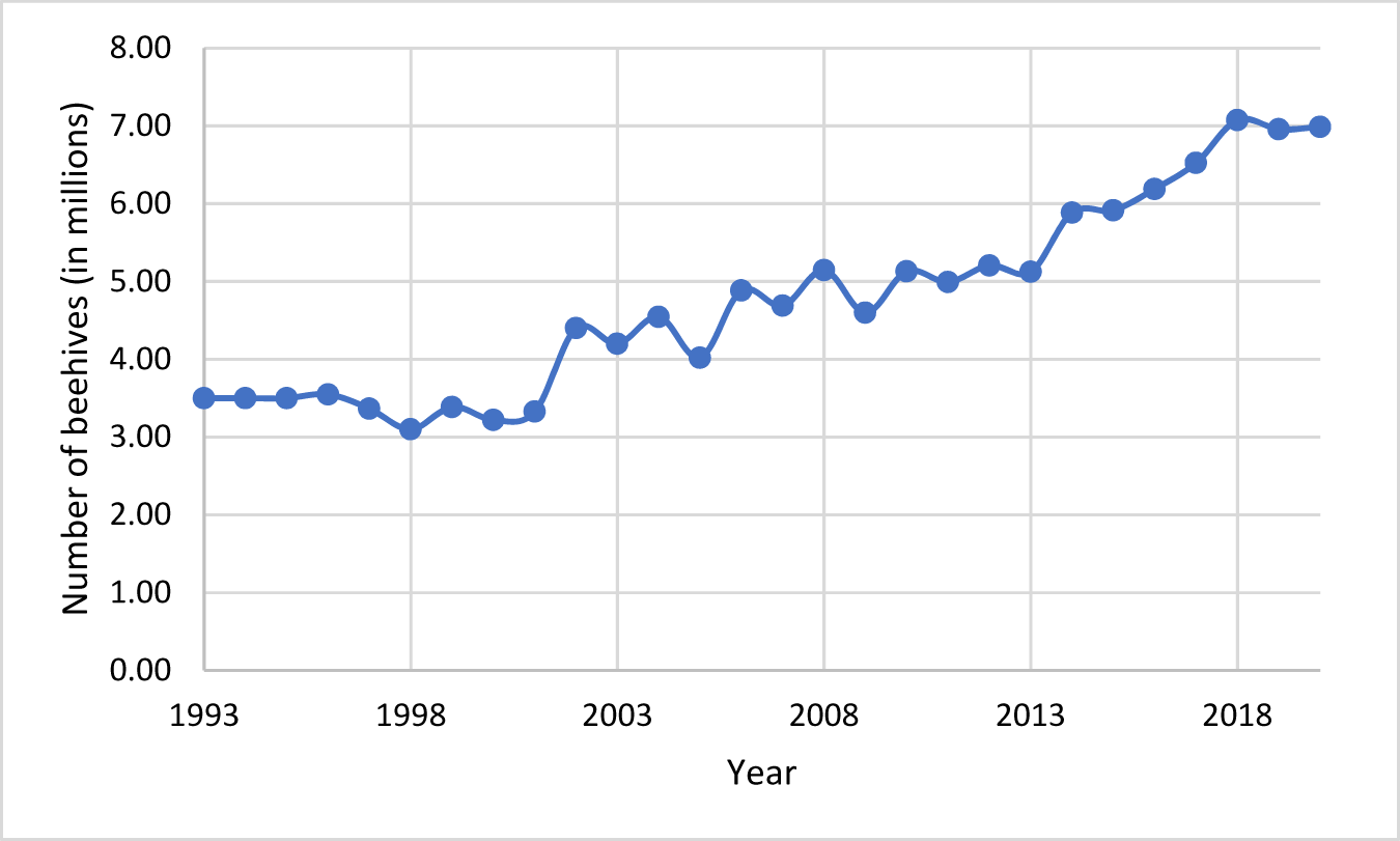
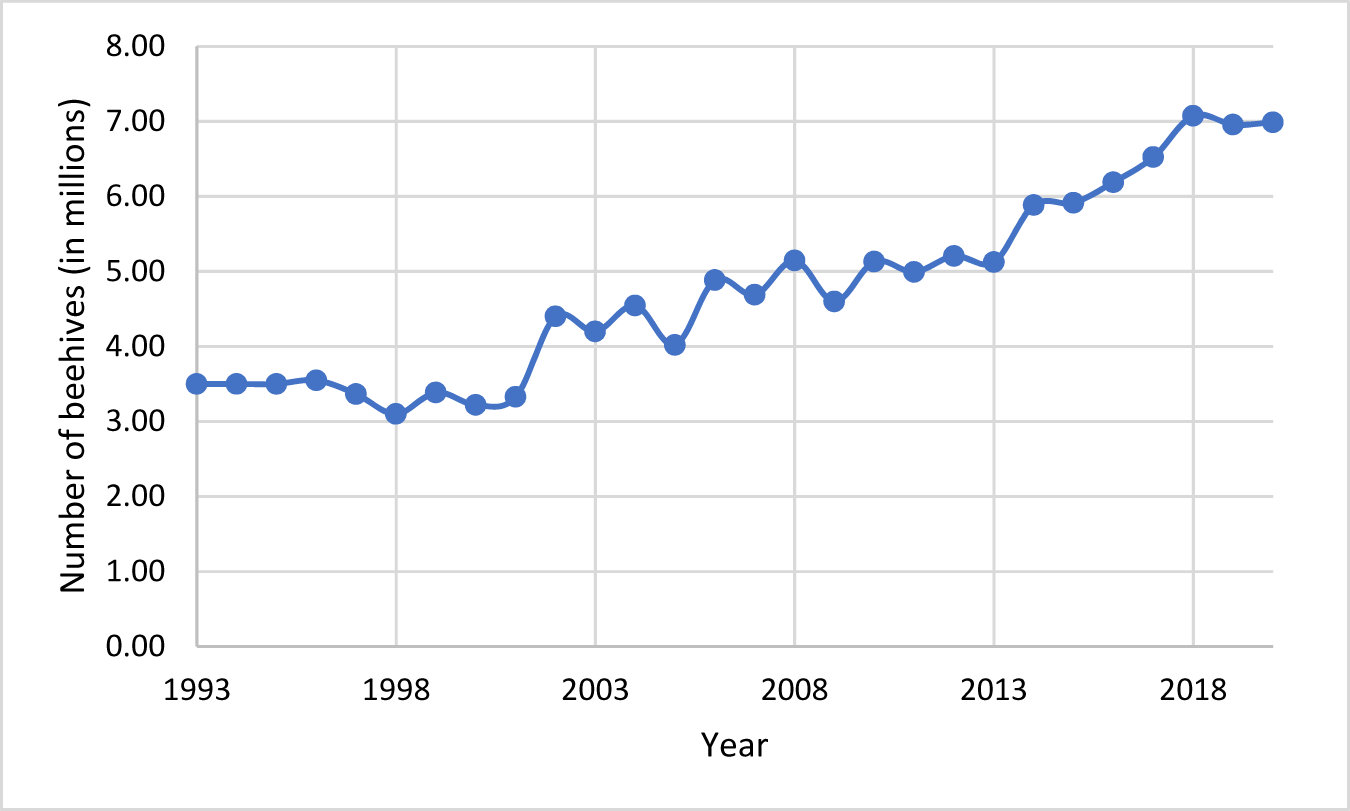
Beekeeping in Ethiopia is a long-standing agricultural practice, with many rural farmers using it as an additional source of income through honey and beeswax production (Gratzer et al., Reference Gratzer, Wakjira, Fiedler and Brodschneider2021). As Figure 1 shows, the number of beehives in Ethiopia has increased steadily since 1993, currently reaching approximately 7 million. Ethiopia is home to the largest number of bee colonies in Africa and ranks fourth in the world in beeswax production and tenth in honey production (Girma and Gardebroek, Reference Girma and Gardebroek2015). The beekeeping industry in Ethiopia produces approximately 84,591 tons of honey per year (FAO, 2025) and employs approximately 2 million people (Drost et al., Reference Drost, Van Wijk and Mandefro2011). The sector has gained significant attention from both the government and development partners, with organizations such as the Mastercard Foundation investing millions of dollars and creating thousands of jobs in the beekeeping sector (Mastercard Foundation, 2019). Beekeeping in Ethiopia also offers opportunities for landless farmers, including many women and young people, to improve their livelihoods (Abro et al., Reference Abro, Kassie, Tiku, Taye, Ayele and Ayalew2022).
Number of beehives in Ethiopia from 1993–2020.
Agriculture accounts for more than 30 per cent of GDP, employs more than 65 per cent of the workforce and earns more than 80 per cent of foreign exchange in Ethiopia. Furthermore, crop production accounts for an average of 60 per cent of the sector’s output, while livestock production accounts for 27 per cent of total agricultural value added (Alemu et al., Reference Alemu, Oosthuizen and Hd2010). Beekeeping accounts for 1.3 per cent of the country’s agricultural GDP (Akessa, Reference Akessa2016). However, low productivity remains a practical and policy challenge. One policy option for raising productivity is to focus on pollinators that have been shown to increase the quality and quantity of PD crop yields (Stein et al., Reference Stein, Coulibaly, Stenchly, Goetze, Porembski, Lindner, Konaté and Linsenmair2017).
Many studies done in Ethiopia have shown the role of bee pollination in improving the yields and quality of crops such as Malus sylvestris (apple), Allium cepa (red onion), Guizotia abyssinica (niger) and Vicia faba (faba beans), with the yield increase ranging between 34 and 84 per cent due to honey bee pollination (Bareke and Addi, Reference Bareke and Addi2019). A prominent example of pollination benefit is a study on apples in Ethiopia comparing trees exposed to bee pollination and caged trees; the results showed a 78 per cent yield advantage when using bee pollinators compared to caged trees (Bareke et al., Reference Bareke, Addi and Wakjira2018), which represents a 78 per cent pollinator dependency ratio. Other crops with high pollinator dependence are avocadoes (65 per cent), mangoes (65 per cent), peppers, soybeans, fenugreek, coffee, cotton and groundnuts (all at 25 per cent) (Alebachew, Reference Alebachew2018).
3. Methods
3.1. Data and measurement
We use five rounds of nationally representative panel data collected by the Ethiopian Statistics Service as part of the World Bank Living Standards Measurement Study – Integrated Surveys on Agriculture (LSMS-ISA) programme. The waves used span the 2011–2012, 2013–2014, 2015–2016, 2018–2019 and 2021–2022 agricultural seasons. The first three waves (2011–2015) follow the same panel of households and therefore admit household FE estimation, whereas the 2018–2019 and 2021–2022 rounds use a different sampling frame; we therefore pool all five waves in our main specifications (which rely on cross-sectional variation within zone and across time), and confine household FE estimation to the 2011–2015 panel as a robustness check. After cleaning, the effective sample contains approximately 10,800 household-year observations across the five waves (about 7,600 for the three-wave household FE subsample). Detailed sampling and questionnaire documentation are available on the World Bank LSMS-ISA website.Footnote 1 The outcome variable is the logarithm of gross crop revenue measured in 2015 constant US dollars. For each household  $i$ in year
 $t$, gross crop revenue is the sum over all crops
 $c$ harvested by the household, of total quantity (
 ${Q_{ict}}$) multiplied by the crop-specific price, p. Prices are constructed using a price hierarchy: where a household reports a sale, we use the household-level sale price; otherwise, we use the median price observed in the household’s woreda (district). Local currency values are first deflated to a common base year (2015) using Ethiopia’s official consumer price index, then converted to US dollars at the 2015 official exchange rate. Because gross crop revenue is right-skewed and contains a non-trivial share of zeros (households reporting no marketable harvest), we use the logarithm of revenue (plus one) as our main outcome variable. As a robustness check, we also report results using the inverse hyperbolic sine transformation (asinh) of revenue. We winsorize the underlying revenue measure at the 1st and 99th percentiles. Pollination services provided by managed bees can improve both the quantity and quality of output (Bommarco et al., Reference Bommarco, Marini and Vaissière2012; Garratt et al., Reference Garratt, Breeze, Jenner, Polce, Biesmeijer and Potts2014; Phalkey et al., Reference Phalkey, Aranda-jan, Marx, Höfle and Sauerborn2015; Stein et al., Reference Stein, Coulibaly, Stenchly, Goetze, Porembski, Lindner, Konaté and Linsenmair2017; Hünicken et al., Reference Hünicken, Morales, García and Garibaldi2020; Chen et al., Reference Chen, Fijen, Kleijn and Scheper2021). As discussed in Section 3.3, we disentangle the pathways through which the benefits of pollination services are realized on crop revenue via yield and quality improvement. We measure yield as total production in kilograms, divided by the land area in hectares planted with a particular crop. To proxy for crop quality, we used the farmers’ reported unit prices of pollinator-independent (PI) and PD crops.
The key independent variable is a binary indicator equal to 1 if household  $i$ in wave
 $t$ lives within 5 km of any beekeeping household (defined as a household reporting at least one occupied beehive in that wave), and 0 otherwise. We construct this measure as follows. In each wave, every surveyed household has GPS coordinates for the centroid of its enumeration area (EA) (the precise plot or homestead location is not released for confidentiality reasons). We treat the EA centroid as the location of every household in that EA and compute the Euclidean (great-circle) distance between every pair of EA centroids using the haversine formula. A household is coded as ‘within 5 km of a beekeeper’ if the EA centroid of a beekeeping household in the same wave lies within 5 km of its own EA centroid. For most, this indicates living within the same EA as the beekeeper, or close by. Importantly, beekeeping households are themselves coded as within 5 km of a beekeeper (i.e., themselves), so the indicator captures both private and external benefits in the main specification; the externality-only specification in Section 4.2 drops beekeeping households from the estimation sample.
The distance travelled by honeybees varies considerably depending on many factors, such as season (Couvillon et al., Reference Couvillon, Schürch and Ratnieks2014), food availability and bee species (Schneider and Hall, Reference Schneider and Hall1997). However, the most-cited references on honeybee foraging report an average radius of 5 km (Beekman and Ratnieks, Reference Beekman and Ratnieks2000). Instead of simply adopting this, we empirically test different radii and find that the highest positive impact on crop revenue occurs at 5 km, after which it begins to decline (Table A1 in the Supplementary Appendix). Thus, we use a 5 km cut-off to reflect the honeybee's maximum foraging range (Beekman and Ratnieks, Reference Beekman and Ratnieks2000; Abrol, Reference Abrol2013). This approach allowed us to link beekeeping activity with agricultural outcomes in a spatially explicit manner. As further reassurance for using the beekeeper’s EA centroid as a proxy for hive location, Ethiopian beekeeping is overwhelmingly stationary, with no significant commercial migratory practice (Gratzer et al., Reference Gratzer, Wakjira, Fiedler and Brodschneider2021); this limits the bias introduced by approximating hive location with the beekeeper’s homestead area. We also report results that simply use an indicator for whether a household lives in the same woreda as a beekeeper and the results are generally the same but with a smaller coefficient.
Because distances are measured between EA centroids rather than between individual homesteads or plots, there is necessarily some measurement error: a household close to the EA boundary may in reality be closer or farther from the nearest beekeeper than the centroid-to-centroid distance implies. This measurement error is, however, plausibly classical and shrinks towards zero as the radius increases. To probe its influence, we (i) vary the radius cut-off (Table A1, Supplementary Appendix), (ii) use the continuous log-distance measure and (iii) report a woreda-level ‘any beekeeper’ indicator, which by construction is invariant to within-EA centroid placement. All three give qualitatively consistent results.
As a measure of the intensive margin of beekeeping in a household’s vicinity, we use the log of the number of beehives reported by all sampled households in the woreda (admin-3 area) in that wave. This serves as a density-style measure of beekeeping intensity surrounding the household. We also report results using the (negative) log distance to the nearest beekeeping household as an alternative continuous intensity measure.
In the subsequent econometric analysis, we control for a set of economic, environmental, farm-level and demographic variables that could confound the relationship between pollination and agricultural earnings. We include annual household expenditure to capture welfare and wealth differences that influence access to inputs and the adoption of pollinator-friendly practices. Wealthier households may manage their farms more intensively and invest in yield-enhancing technologies, thus indirectly affecting pollination outcomes. We also control for education level and age of the household head to account for human capital and experience, which shape decision-making and openness to innovation. Household size in adult-equivalent terms can capture labour availability for farm operations, while livestock ownership can reflect asset endowments and livelihood diversification. Participation in agricultural extension programmes is included to control for exposure to new knowledge and technologies that could improve crop management and pollination outcomes.
We further account for farm size and the use of agricultural inputs – fertilizers, improved seeds and agrochemicals – because these factors influence crop productivity and interact with pollination services. Larger farms may benefit from economies of scale or face management challenges that affect pollination efficiency. Similarly, chemical input use and seed types can either complement or hinder pollinator activity, making it important to isolate their independent effects on gross revenue. Finally, we include environmental and landscape variables such as the percentage of forest cover in the district to capture ecological and climatic heterogeneity that affects crop productivity. We use forest cover from the Global Forest Watch for 2000, as it is not available for more recent years (Hansen et al., Reference Hansen, Potapov, Moore, Hancher, Turubanova, Tyukavina, Thau, Stehman, Goetz, Loveland, Kommareddy, Egorov, Chini, Justice and Townshend2013). We use the annual mean temperature and total annual rainfall because Ethiopia has bimodal rainfall in most parts, and crops benefit from residual moisture that may accumulate in the non-growing season. Forests enhance pollinator habitats, while rainfall and temperature affect flowering patterns and foraging behaviour. Annual climatic variables are also important because they can affect honeybee behaviour and the forests upon which they depend for foraging. By controlling for these diverse factors, we ensure that our estimated impact of pollination on gross crop revenue reflects its contribution rather than the influence of confounding socioeconomic or environmental conditions.
We obtained the environmental and landscape-level variables from various sources. The rainfall and temperature variables are included in the LSMS-ISA. The World Bank and country statistical offices use GPS coordinates from household survey data to link household data to rainfall and temperature data from the National Oceanic and Atmospheric Administration Climate Prediction Center.
3.2. Descriptive statistics
Table 1 summarizes all the key variables that describe our sample, tested by whether the household lives within the 5-km radius of a beekeeper. All monetary values are adjusted for inflation to 2015 prices. About 27 per cent of the interviewed household farms were within a 5-km radius of a beekeeper. As Table 1 further demonstrates, almost all explanatory variables differ by household treatment status (living within a 5-km radius).
Summary statistics of the main variables
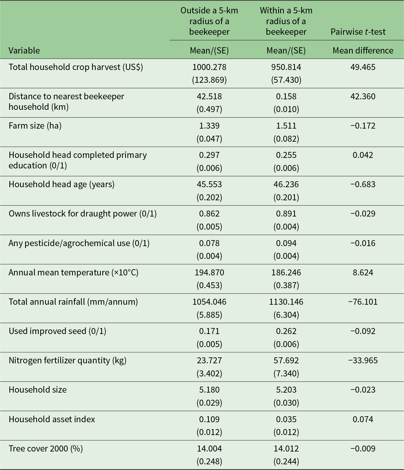
Table 1 Long description
Mean values with standard errors are reported for households outside a 5 km radius of a beekeeper and within a 5 km radius, alongside a pairwise t test column of mean differences. Total household crop harvest averaged 1000.278 US dollars outside and 950.814 within, with a mean difference of 49.465. Farm size averaged 1.339 hectares outside and 1.511 within, with a mean difference of minus 0.172. Household head completed primary education averaged 0.297 outside and 0.255 within, with a mean difference of 0.042, and household head age averaged 45.553 years outside and 46.236 within, with a mean difference of minus 0.683. Owns livestock for draught power averaged 0.862 outside and 0.891 within, and any pesticide or agrochemical use averaged 0.078 outside and 0.094 within. Annual mean temperature averaged 194.870 in units of ten degrees Celsius outside and 186.246 within, and total annual rainfall averaged 1054.046 millimeters per annum outside and 1130.146 within. Used improved seed averaged 0.171 outside and 0.262 within, nitrogen fertilizer quantity averaged 23.727 kilograms outside and 57.692 within, household size averaged 5.180 outside and 5.203 within, household asset index averaged 0.109 outside and 0.035 within, and tree cover 2000 averaged 14.004 per cent outside and 14.012 within.
Note: Standard errors in parentheses.
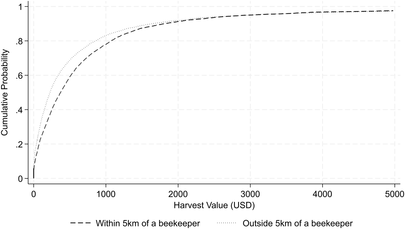
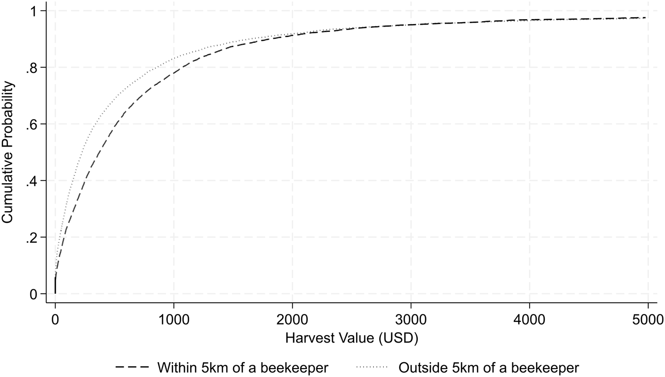
The gross crop revenue or harvest value of farmers residing within a 5-km radius of at least one beekeeper is lower by US$50 per year, but not significantly so, compared to those living outside this radius. We further draw the cumulative distribution by the household status (Figure 2). Along the distribution, the difference in gross income appears to be nearly zero at both tails. However, in the middle of the distribution, we observe a clear difference in gross crop income: households living more than 5 km from at least one beekeeper have higher income. These two cumulative distribution functions differ significantly based on Kaplan's (Reference Kaplan2019) approach. The global test result shows a simulated p-value < 0.0001, indicating strong evidence against the null hypothesis of equality between the two distributions.
Cumulative distribution of gross crop income (harvest value) by whether the household lives within 5 km of beekeeper or not.
3.3. Empirical specifications
To estimate the impact of beekeeping on gross crop revenue for household  $i$ in village (EA)
 $v$ at time
 $t$ (
 ${y_{ivt}}$), we use the model
 \begin{equation}{y_{ivt}} = \beta H{B_{ivt}} + \theta {X_{ivt}} + \omega {D_{vt}} + \vartheta {S_t} + \gamma {Z_i} + {\alpha _i} + {\text{ }}{{{\xi }}_{ivt}}\end{equation}
where  ${y_{ivt}}$ is the logarithm of gross crop income in US$; log-transforming
 ${y_{ivt}}$ helps make relationships more linear, reduces influence of outliers and allows us to interpret the results in percentage changes;
 $H{B_{ivt}}$ is a dummy variable equal to 1 if household
 $i$ in EA
 $v$ lives within a radius of 5 km from a household managing honeybees at time
 $t,$ and 0 otherwise.
 ${X_{it}}$ represents vector of household characteristics controlled in the regression (see Table 1 for all variables);
 ${D_{vt}}$ is a vector of environmental variables including rainfall, temperature and forest cover that are at the EA level.
 $S$ and
 $Z$ are vectors of survey years and zone FE, respectively.
 ${\alpha _i}$ is the household FE in a two-way FE specification that includes the household FE. In Equation (1), our parameter of key interest is, which quantifies the impact of beekeeping through pollination on crop production. We expect the
 $\beta $ to be positive and statistically significant.
 ${{{\xi }}_{ivt}}$ is the error term. Standard errors are clustered at the household level, the unit of analysis. The number of household clusters in the analytical sample is well above conventional thresholds for cluster-robust inference. We do not implement multiway clustering in the main specification because the treatment varies at the household-by-community-proximity level and the panel structure makes within-household serial correlation the primary concern.
We adopt a sequential estimation approach to assess the robustness of our findings, beginning with a parsimonious pooled OLS specification that includes only zone and year FE, and then a model with all the controls included. This sequential approach allows us to examine the stability of coefficient estimates by controlling for additional covariates, which provides insight into the potential severity of omitted variable bias (Altonji et al., Reference Altonji, Elder and Taber2005). If the coefficient on our key explanatory variable – proximity to beekeepers – remains relatively stable across specifications with different sets of controls, it suggests that selection on observables adequately addresses confounding and that remaining selection on unobservables is likely to be limited.
While the two-way FE (with household FE) specification is often considered the standard in panel data analysis, as it requires less strong assumptions about the nature of unobserved heterogeneity, it is not without limitations, particularly when the treatment variable exhibits minimal within-unit variation over time. When household proximity to beekeepers changes infrequently, FE estimators may suffer from severe attenuation bias due to the amplification of measurement error in the demeaned data (Griliches and Hausman, Reference Griliches and Hausman1986; Debela et al., Reference Debela, Gehrke and Qaim2021). For example, in our data, the within (year-to-year within the same household) variation in the key variable, living within 5 km of a beekeeper, only varies by about 11 per cent across the years. Moreover, the FE transformation does not use cross-sectional variation, relying exclusively on potentially noisy temporal deviations from household-specific means. As Angrist and Pischke (Reference Angrist and Pischke2009) emphasized, FE are not universally superior to pooled OLS and can actually increase bias when key variables display limited time variation, effectively throwing away valuable identifying information. Our key policy variable of interest does not vary much over time (80 per cent of the EAs maintain their 1-year status throughout); the household status, whether they live within or outside the 5-km radius, does not change significantly over the survey years. Furthermore, in our data, the panel is maintained for only three waves, and then again for the last two waves. However, we do not simply rely on this theoretical weakness of the FE approach to dismiss it entirely. Instead, as a further robustness check, we re-estimate (1) on the 2011–2015 subsample (the longer wave), adding household FE. The results are generally confirmed.
However, our preferred specification is the pooled OLS model with comprehensive controls, zone FE, year FE and input-use variables. This approach balances concerns about omitted variable bias with the practical reality that treatment assignment exhibits limited within-household variation. We use zone FE as the main geographic control because they absorb broad, persistent spatial differences in agroecology, market access, institutions and agricultural potential, while still preserving the within-zone cross-community variation in nearby beekeeper exposure needed for identification. Finer FE such as EA, village/kebele or woreda would absorb much of the local variation in beekeeper presence and distance that defines the treatment. The rich set of household and input controls further mitigates concerns about selection on observables.
To isolate the pure external benefit of beekeeping for non-beekeeping households, we re-estimate (1) on the subsample of households that report owning zero beehives in wave  $t$. Conceptually, beekeepers themselves benefit from both their own colonies and from any other beekeepers in the vicinity, so the all-household estimate of the
 $\beta $ blends a private and a social effect. Restricting to non-beekeepers cleanly identifies the externality and additionally addresses concerns that the decision to keep bees is endogenous to expected agricultural income.
3.4. Impact pathways: improvement in quality and/or yield?
As stated earlier, managed honeybees can improve agricultural income by increasing yield and/or quality of output. We test these two impact channels to understand how beekeeping affects crop revenue. We begin by testing the impact of beekeeping on yield. We assess the effect of beekeeping on the top six crops: three PD and three PI. This follows other studies that determine the impact of bees’ pollination on crop yields (Stein et al., Reference Stein, Coulibaly, Stenchly, Goetze, Porembski, Lindner, Konaté and Linsenmair2017; Reilly et al., Reference Reilly, Artz, Biddinger, Bobiwash, Boyle, Brittain, Brokaw, Campbell, Daniels, Elle, Ellis, Fleischer, Gibbs, Gillespie, Gundersen, Gut, Hoffman, Joshi, Lundin, Mason, McGrady, Peterson, Pitts-singer, Rao, Rothwell, Rowe, Ward, Williams, Wilson, Isaacs and Winfree2020). The data used to test the impact pathways are at the crop level, and some households have more than one plot of the same crop.
We do not separately re-estimate gross crop revenue restricted to PD-only or PI-only subsamples. The reason is that households frequently switch their crop mix across waves, and a large majority of household-years feature only PI crops, so the PD-only revenue sample becomes severely unbalanced across households and waves, undermining the panel structure needed for our pooled OLS with zone-and-year FE estimator. We instead exploit the PD/PI contrast directly at the crop level in Section 4.3, which is the more informative test of the differential effect that pollination should have on PD versus PI crops. We estimate the pooled OLS model using Equation (2) as follows:
 \begin{equation}Q_{civ}=\gamma_1HB_{iv}+\gamma_2M_{cif}+\gamma_3X_i+\alpha_i+\tau_{civ,}\end{equation}
where  $Q_{civ}$ is the yield for crop
 $c$,
 $M_{cif}$ is a vector of plot-level (f) controls such as slope, the distance of the plot to the homestead and plot elevation;
 $\tau_{civ}$ is the error term at the plot level;
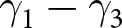 ${\gamma _1} - {\gamma _3}$ are parameters to be estimated; the parameter of interest is
 ${\gamma _1}$ showing the impact of beekeeping on the yield of crop
 $c$; and the rest of the variables remain as defined in Equation (1). We cluster the errors at the household level as before.
We estimate Equation (2) for the top three PI crops (maize, sorghum and Teff) and PD crops (sesame, pumpkins and red pepper). We select the top three PI and PD crops in the dataset based on their frequency and land size. For PD crops, we restrict the estimation to annual crops because they have better yield measurement, as they are harvested at once, and the price at the time of the survey is more reflective of the main price. Furthermore, annual crops exhibit better relationships among yield, pollination and other inputs, as there is no residual effect carried over to the next year. We have used the pollinator dependency classification to categorize crops as PD or PI (Klein et al., Reference Klein, Vaissière, Cane, Steffan-dewenter, Cunningham, Kremen and Tscharntke2007). Klein et al. (Reference Klein, Vaissière, Cane, Steffan-dewenter, Cunningham, Kremen and Tscharntke2007) define pollinator dependency as whether the quantity of fruits and seeds produced changes due to pollinators. We categorized all crops with some level of pollinator dependency as PD, and those without any level of dependency as PI.
Next, we quantify whether households that live in communities with managed honeybees fetch a higher price for their PD crops. Equation (3) shows the estimated pooled OLS model,
 \begin{equation}p_{civ}= \beta_1HB_{iv}+\beta_2PD_c+ \beta_3BH_{iv}\cdot PD_c+\beta_4X_{iv}+\alpha_i+e_i,\end{equation}
where  $p_{civ}$ is village-level price of crop
 $c$,
 $P{D_c}$ is an indicator of pollinator dependency (with 1 = PD crop, 0 otherwise),
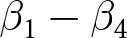 ${\beta _1} - {\beta _4}$ are parameters to be estimated,
 ${e_i}$ is the idiosyncratic error term and the remaining variables are as defined in Equations (1) and (2). The standard errors in Equation (3) are clustered at the household level.
 ${\beta _3}$ is the main parameter of interest. It shows the effect of beekeeping on the prices of PD and PI crops. If PD crops fetch better prices, the coefficient (
 ${\beta _3}$) must be positive and statistically significant.
We use price per kg as a proxy for quality (Bils and Klenow, Reference Bils and Klenow2001; Panzone, Reference Panzone2012). In the data, we have no measure of crop output quality, such as grading or sorting the output, particularly for horticultural crops. Therefore, we rely on the per-unit price as a proxy for quality. If managed bees positively impact the quality of the produce in a given village, we expect that the output sold from those villages will, on average, fetch a higher price.Footnote 2 Studies on various crops show that buyers are willing to pay higher prices for higher-quality produce in Ethiopia (Abate and Bernard, Reference Abate and Bernard2017; Minten et al., Reference Minten, Assefa and Hirvonen2017; Abewa et al., Reference Abewa, Adgo, Alemayehu, Yitaferu, Assefa and Cools2021). Inferring the value of pollination through a premium for better quality has also been used in other studies. For example, Klatt et al. (Reference Klatt, Holzschuh, Westphal, Clough, Smit, Pawelzik and Tscharntke2014) and Wietzke et al. (Reference Wietzke, Westphal, Gras, Kraft, Pfohl, Karlovsky, Pawelzik, Tscharntke and Smit2018) sorted strawberries by quality (e.g., colour, blemishes) and found that insect-pollinated strawberries had higher quality and fetched higher prices in the European market. Garratt et al. (Reference Garratt, Breeze, Jenner, Polce, Biesmeijer and Potts2014) traced both the farmgate price and the final price paid by consumers and found similar results – bee-pollinated apples fetched higher prices because they were larger and of better shape.
4. Results
4.1. Main results
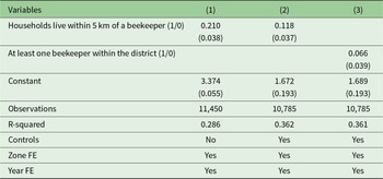
We begin by presenting the impact of beekeeping on gross crop income. For brevity, the full regression results for our preferred model are reported in Table A2 (Supplementary Appendix). Table 2 reports the coefficients associated with our key policy variable, whether households live within 5 km of at least one beekeeper. We begin with the pooled OLS without controls. As shown in column (1), without any controls and only the zone and year FE, the coefficient is much larger and likely biased upward. When we add more controls, the effect size decreases from approximately 21 to 12 per cent. We find that the effect of managed bees on crop revenue is sensitive to whether confounding factors are included or excluded. When we control for observed characteristics, including location and survey-year FE, the coefficient on our policy variable drops by about 10 percentage points.
Impact of beekeeping on household crop revenue (log, US$ per year)
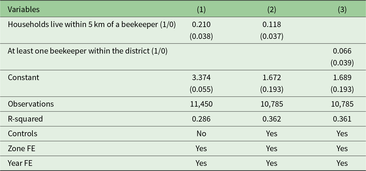
Table 2 Long description
The outcome is household crop revenue measured as a log value in US dollars per year, reported across three models in columns 1, 2, and 3. Column 1 lists, effect of whether a household lives within 5 km of a beekeeper, coefficient 0.210 with standard error 0.038, and a constant of 3.374 with standard error 0.055. Column 2 lists the same 5 km variable with coefficient 0.118 and standard error 0.037, and a constant of 1.672 with standard error 0.193. Column 3 replaces the 5 km variable with at least one beekeeper within the woreda, coefficient 0.066 with standard error 0.039, and a constant of 1.689 with standard error 0.193. Observations are 11,450 in column 1 and 10,785 in columns 2 and 3. R-squared values are 0.286 in column 1, 0.362 in column 2, and 0.361 in column 3. Controls are No in column 1 and Yes in columns 2 and 3, while Zone FE and Year FE are Yes in all three columns.
Notes: Column (3) re-estimates the main pooled OLS with zone and year FE specification (column (2)) substituting an indicator for living within a 5-km radius of at least one beekeeper in the district. Controls and FE in column (3) are the same as in column (2). Standard errors clustered at the household level in parentheses.
‘Controls’ includes the following household, input-use and environmental covariates: household head completed primary education (0/1), household head age (years), ownership of livestock for draught power (0/1), use of any pesticide/agrochemical (0/1), use of improved seed (0/1), nitrogen fertilizer quantity (kg), household size, household asset index, annual mean temperature (°C), total annual rainfall (mm) and tree cover in 2000 (%).
All subsequent tables use the same set of controls; for brevity, the list is not repeated.
Column (3) shows that the result is not specific to the 5-km radius construction. When we instead use a binary indicator equal to 1 if any household in the woreda reports keeping bees, the effect is about 7 per cent, indicating that it diminishes as the area considered for treatment expands. The smaller coefficient here is expected: the district indicator includes households whose nearest beekeeper is more than 5 km away (and hence likely outside foraging range), attenuating the average effect.
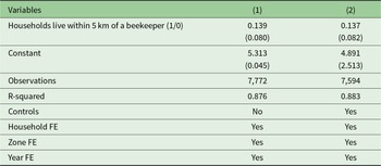
Our preferred specification is therefore the pooled OLS model with the full set of controls (column (2)). The coefficient implies that living within 5 km of a beekeeper raises gross crop revenue by about 12 per cent. Evaluated at the sample-mean gross crop revenue (approximately US\$1,000 per household per year), this corresponds to roughly US\$120 per year per treated (within 5km radius) household. The household FE robustness check on the longer panel (Table 5) returns a similar point estimate (about 14 per cent, marginally significant at the 10 per cent level), confirming that the result is not driven by time-invariant unobserved heterogeneity across households and that the loss of identifying variation under household FE is not so severe as to overturn the qualitative finding.
Table A1 (Supplementary Appendix) reports the sensitivity of the main estimate to alternative radius cut-offs. The coefficient is essentially flat between 0, 2, 3 and 5 km (all roughly 0.12, p < 0.01), then falls to 0.078 at 7 km (p < 0.05) and to a statistically insignificant 0.047 at 10 km. This pattern is precisely what one would expect from the foraging biology: the effect should be strongest at distances within the typical honeybee foraging range and decay thereafter.
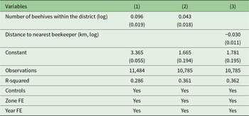
Table 3 reports the intensive margin estimates. Two measures of intensity are used. First, the logarithm of the number of beehives reported by sampled households in their district captures the density of managed colonies in the immediate vicinity. Second, the logarithm of the distance to the nearest beekeeper (where smaller values indicate greater exposure) captures the intensity of proximity. The logarithm of beehives is significantly positive in both the without-controls and fully controlled specifications: a 10 per cent increase in the number of colonies raises gross crop revenue by roughly 0.4 per cent. The log distance to the nearest beekeeper shows a negative and statistically significant coefficient. Doubling the distance from the nearest beekeeper reduces gross crop revenue by approximately 3 per cent. These results provide robust evidence that the intensive margin matters too.
Impact of beekeeping on agricultural value – intensive margin
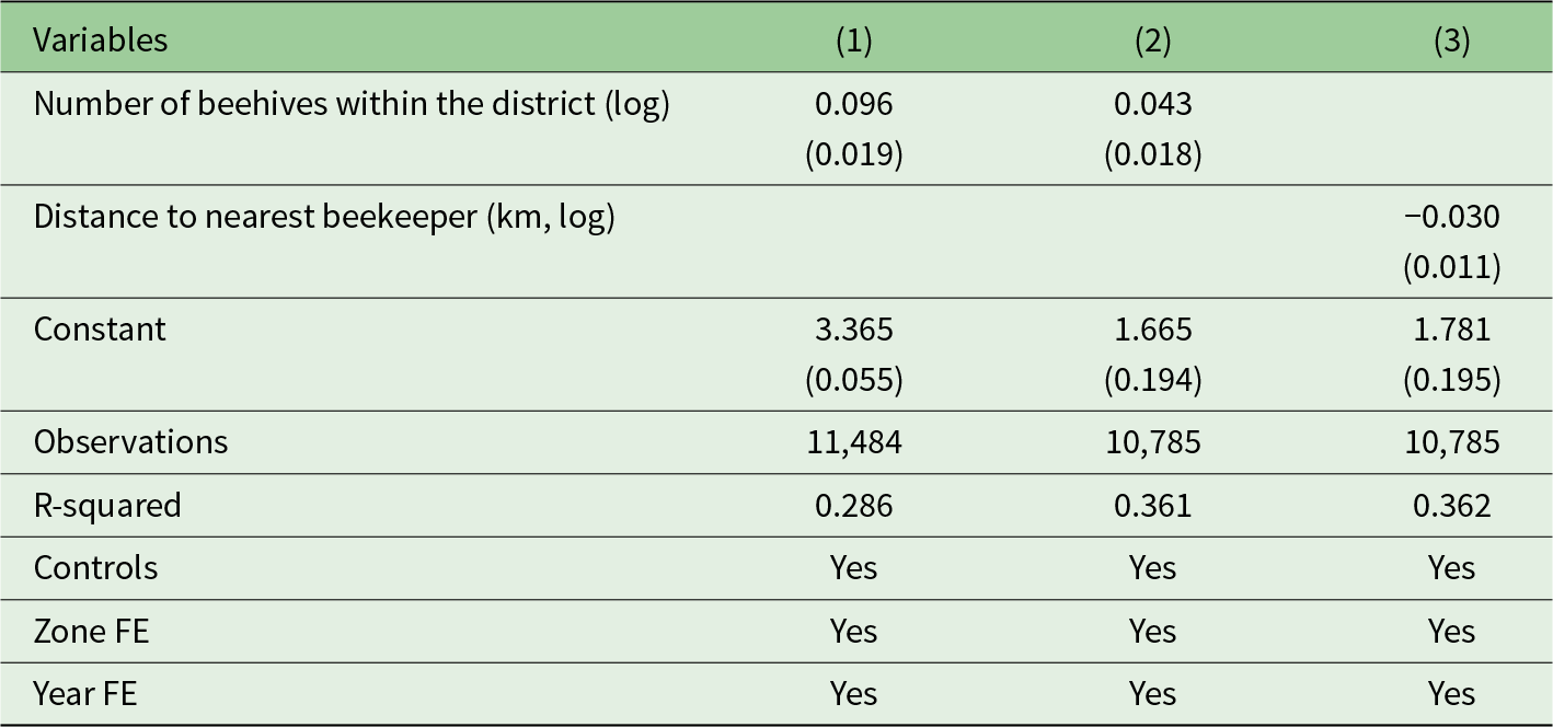
Table 3 Long description
Three regression models in columns 1 to 3 report coefficients with standard errors in parentheses for two beekeeper proximity measures, plus a constant and model statistics. For number of beehives within the district, log, the coefficient is 0.096 with standard error 0.019 in column 1, and 0.043 with standard error 0.018 in column 2; this variable is not reported in column 3. For distance to nearest beekeeper in kilometers, log, the coefficient is minus 0.030 with standard error 0.011 in column 3; this variable is not reported in columns 1 or 2. The constant is 3.365 with standard error 0.055 in column 1, 1.665 with standard error 0.194 in column 2, and 1.781 with standard error 0.195 in column 3. Observations are 11,484 in column 1 and 10,785 in columns 2 and 3. R squared is 0.286 in column 1, 0.361 in column 2, and 0.362 in column 3. Controls, zone FE, and year FE are marked Yes in all three columns.
Notes: Controls are the same as in Table 2. ‘Number of beehives within the district (log)’ is the log of the total number of beehives reported by surveyed households in the household’s woreda in that wave; ‘Distance to nearest beekeeper (km, log)’ is the log of the EA-centroid-to-EA-centroid distance to the nearest household reporting beehives. Estimation uses pooled OLS. Standard errors clustered at the household level in parentheses.
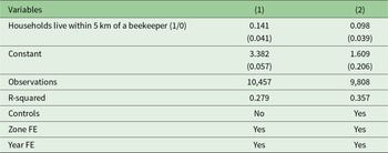
Households that do not keep bees do not incur the private costs of beekeeping, while enjoying social benefits. We estimate these social benefits or positive externalities. The results in Table 2 include households that keep bees and those that do not within the same area. Table 4 estimates the same model using pooled OLS but excludes households that keep bees in each area. This regression helps us capture the pure external benefits of managed bees at the household level by excluding households that keep bees. Furthermore, if potential concerns remain regarding the endogenous decision to keep honeybees, it also helps to address this challenge, as beekeepers’ decisions are exogenous to other households in the area.
Pure externality impact of beekeeping on crop revenue of households (log of US$) (excluding the owners of beehives)
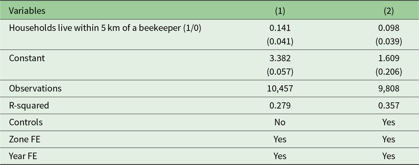
Table 4 Long description
Outcome is crop revenue measured as the log of US dollars, reported for households with zero beehives. Two models in columns 1 and 2. In column (1), households living within 5 km of a beekeeper (1/0), the coefficient is 0.141 with standard error 0.041, and 0.098 with standard error 0.039 in column 2. The constant is 3.382 with standard error 0.057 in column 1, and 1.609 with standard error 0.206 in column 2. Observations are 10,457 in column 1 and 9,808 in column 2. R-squared is 0.279 in column 1 and 0.357 in column 2. Controls are No in column 1 and Yes in column 2, while Zone FE and Year FE are Yes in both columns.
Notes: Sample restricted to households reporting zero beehives in the survey wave. Controls (column (2)) are the same as in Table 2. Standard errors clustered at the household level in parentheses.
The coefficient on the 5 km indicator falls modestly (from 0.118 to 0.098), consistent with the intuition that non-beekeepers should capture most but not all of the social benefit; beekeepers themselves additionally benefit from the pollination of their own colonies. The implied pure-externality gain for non-beekeepers is roughly 9.8 per cent of gross crop revenue, or approximately US$98 per treated household per year. This is, to our knowledge, the first farm-level estimate of the pure pollination externality from managed bees in a low-income country setting. The results reported in Tables 2 and 4 show that beekeeping benefits not only beekeeping households but also other farmers living within a 5-km radius, as bees provide pollination services.
As a robustness check, we also estimate the effect using two-way FE, restricting the sample to the longer panel. Table 5 reports the household-FE specification on the three-wave 2011–2015 panel. Despite the loss of identifying cross-sectional variation noted in Section 3.2, the coefficient on within-5 km exposure remains positive and is nearly identical to the pooled OLS estimate, but is marginally significant at the 10 per cent level. Even when we identify the effect of the relatively rare within-household switches in proximity status, we recover a similar quantitative effect.
Impact of beekeeping on agricultural value using two-way fixed effects
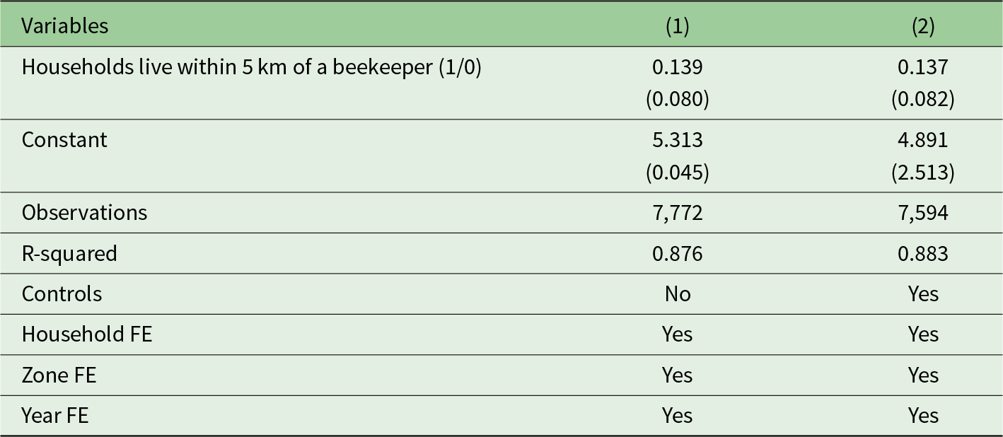
Table 5 Long description
Two regression columns report coefficients for the variable, households living within 5 km of a beekeeper, and a constant, along with observations, R-squared, and fixed effects settings. In column 1, the coefficient for Households live within 5 km of a beekeeper is 0.139 with standard error 0.080, and the constant is 5.313 with standard error 0.045. Column 1 lists 7,772 observations and an R-squared of 0.876, with Controls marked No. In column 2, the constant is 4.891 with standard error 2.513. Column 2 lists 7,594 observations and an R-squared of 0.883, with Controls marked Yes. Household FE, Zone FE, and Year FE are marked Yes in both columns.
Notes: These results are estimated with only the first three waves which is the longer panel.
Controls (column (2)) are the same as in Table 2. Standard errors clustered at the household level in parentheses.
4.2. Economic contribution of beekeeping through pollination services in Ethiopia
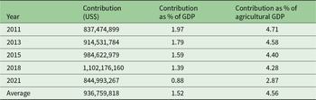
We conducted a back-of-the-envelope calculation to estimate the national-level economic contribution of beekeeping through pollination services using the results from Table 2. First, we calculate the number of farming households living within 5 km of at least one beekeeper, considering only rural households engaged in agriculture, and using the World Bank’s population, GDP and agriculture value-added data in US$. We then multiply the household-average annual benefit of living within 5 km of a beekeeper (i.e., 12 per cent of US\$1000 = US\$120) to obtain the national benefit from beekeeping. We then compute this as a contribution to the total and agricultural GDP share.
The results in Table 6 indicate that managed bees contribute, on average, about US$940 million per year, representing about 1.5 per cent of the GDP and 4.6 per cent of the agricultural GDP. This estimate is within the range of Alebachew (Reference Alebachew2018), who reported that managed bees’ economic contribution through pollination in Ethiopia was about $815 million, representing about 6.3 per cent of agricultural GDP in 2015. This minor difference could be attributed to differences in the estimation approaches used and the period under consideration. This is also within the range of the income benefits of beekeeping (1.3 per cent of GDP), an official figure from Ethiopia's Ministry of Agriculture (Akessa, Reference Akessa2016).
Economic contribution of managed bees in Ethiopia
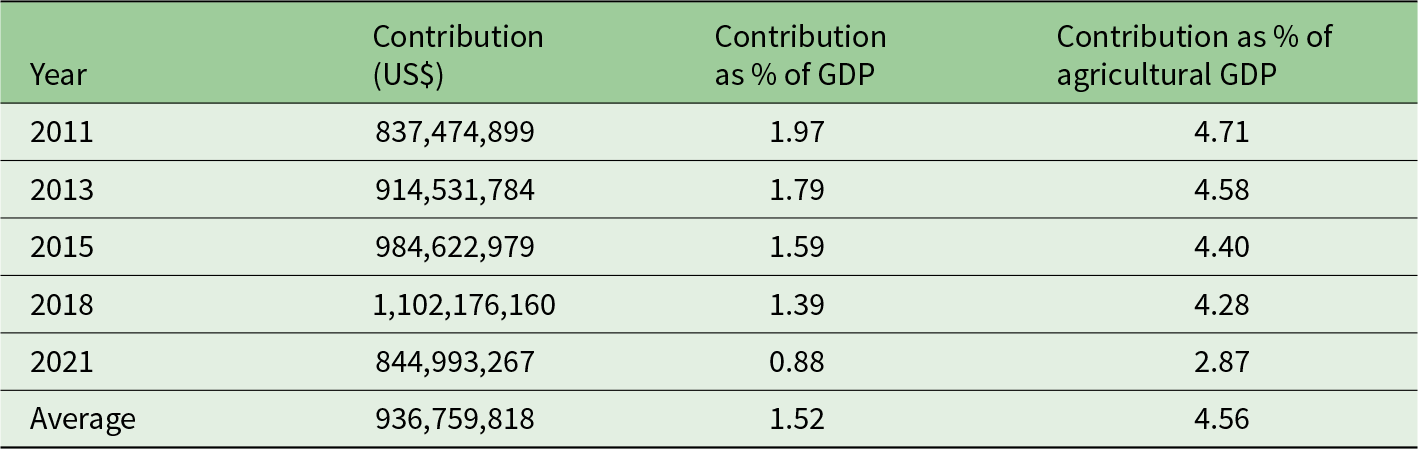
Table 6 Long description
Managed bees economic contribution is listed by year with three columns: Contribution in US dollars, Contribution as per cent of GDP, and Contribution as per cent of agriculture GDP. For 2011, the contribution is 837,474,899, with 1.97 per cent of GDP and 4.71 per cent of agriculture GDP. For 2013, the contribution is 914,531,784, with 1.79 per cent of GDP and 4.58 per cent of agriculture GDP. For 2015, the contribution is 984,622,979, with 1.59 per cent of GDP and 4.40 per cent of agriculture GDP. For 2018, the contribution is 1,102,176,160, with 1.39 per cent of GDP and 4.28 per cent of agriculture GDP. For 2021, the contribution is 844,993,267, with 0.88 per cent of GDP and 2.87 per cent of agriculture GDP. The Average row lists 936,759,818, with 1.52 per cent of GDP and 4.56 per cent of agriculture GDP.
4.3. Impact mechanism: improvement in yield and/or quality?
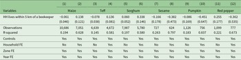
As stated earlier, we hypothesize that the yield benefit will accrue to the PD crops more than the PI crops (Bommarco et al., Reference Bommarco, Marini and Vaissière2012; Garratt et al., Reference Garratt, Breeze, Jenner, Polce, Biesmeijer and Potts2014; Tibesigwa et al., Reference Tibesigwa, Siikamäki, Lokina and Alvsilver2019). Table 7 reports yield-impact estimates for the six crops (maize, teff, sorghum, sesame, pumpkin and red pepper). Among the PI staples, the effect on maize is negative and insignificant in the pooled OLS specification, and on teff it is slightly positive but not robust to household FE. Sorghum shows a small negative coefficient. Among the PD crops, sesame and pumpkin show positive coefficients in at least one specification. For red pepper, the coefficient is negative on average but imprecise. Within the household specifications, precision falls (as expected given the small effective sample size per crop in the three-wave panel), but the signs broadly hold. These results are consistent with the literature documenting heterogeneous, often modest plot-level yield gains from honeybee pollination in real-world African settings (Stein et al., Reference Stein, Coulibaly, Stenchly, Goetze, Porembski, Lindner, Konaté and Linsenmair2017) and also consistent with our finding of a more pronounced effect at the household-aggregated revenue level: small per-crop yield gains across multiple PD crops in a mixed cropping system can aggregate to meaningful household revenue gains. However, the results are mixed and inconsistent overall.
Impact of beekeeping on the logarithm of crop yield for the top three PI and PD crops
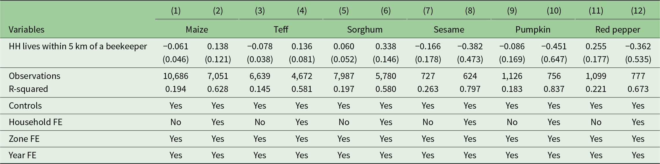
Table 7 Long description
Coefficients and clustered standard errors are reported for the variable, HH lives within 5 km of a beekeeper, across 12 model columns for six crops. Columns 1 and 2 report Maize with coefficients minus 0.061 and 0.138 and standard errors 0.046 and 0.121. Columns 3 and 4 report Teff with coefficients minus 0.078 and 0.136 and standard errors 0.038 and 0.081. Columns 5 and 6 report Sorghum with coefficients 0.060 and 0.338 and standard errors 0.052 and 0.146. Columns 7 and 8 report Sesame with coefficients minus 0.166 and minus 0.382 and standard errors 0.178 and 0.473. Columns 9 and 10 report Pumpkin with coefficients minus 0.086 and minus 0.451 and standard errors 0.169 and 0.647. Columns 11 and 12 report Red pepper with coefficients 0.255 and minus 0.362 and standard errors 0.177 and 0.535. Observations by column are 10,686, 7,051, 6,639, 4,672, 7,987, 5,780, 727, 624, 1,126, 756, 1,099, and 777, with R-squared values 0.194, 0.628, 0.145, 0.581, 0.197, 0.580, 0.263, 0.797, 0.183, 0.837, 0.221, and 0.673. Controls are Yes in all columns, household fixed effects are No in odd numbered columns and Yes in even numbered columns, and zone fixed effects and year fixed effects are Yes in all columns.
Notes: Each pair of columns reports the impact on log yield (kg/ha) for the indicated crop. Odd-numbered columns are the pooled OLS specification with zone and year FE estimated on all five waves; even-numbered columns add household FE on the longer (2011, 2013, 2015) sub-panel. Controls are the same as in Table 2, with the addition of plot-level controls: plot distance from homestead (km), plot elevation (metres above sea level), plot slope (flat, gentle, steep) and plot wetness. Standard errors clustered at the household level in parentheses.
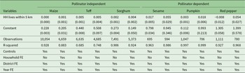
Table 8 reports the corresponding regressions for unit prices (US$/kg). The pattern is much more consistent than it was for yield: for PD crops (sesame, pumpkin and red pepper), the coefficient on proximity to a beekeeper is positive and statistically significant across most specifications – farmers in beekeeping vicinities receive significantly higher unit prices for their PD output. For the PI staples, the price effects are small and largely insignificant. This pattern is consistent with the hypothesis that pollination services improve the quality (size, shape and uniformity) of PD crops, which in turn fetches higher prices in local markets – a quality channel that has been documented for European apples and strawberries (Garratt et al., Reference Garratt, Breeze, Jenner, Polce, Biesmeijer and Potts2014; Klatt et al., Reference Klatt, Holzschuh, Westphal, Clough, Smit, Pawelzik and Tscharntke2014). However, even though we use price as a proxy for quality, sorting crops for their quality is uncommon in African markets. However, for most horticultural products like pumpkin and red pepper, sorting and grading based on size and quality is common even in informal markets (Eaton et al., Reference Eaton, Meijerink and Bijman2008).
Impact of beekeeping on the quality of produce using the log of price (US$) per kg as a proxy
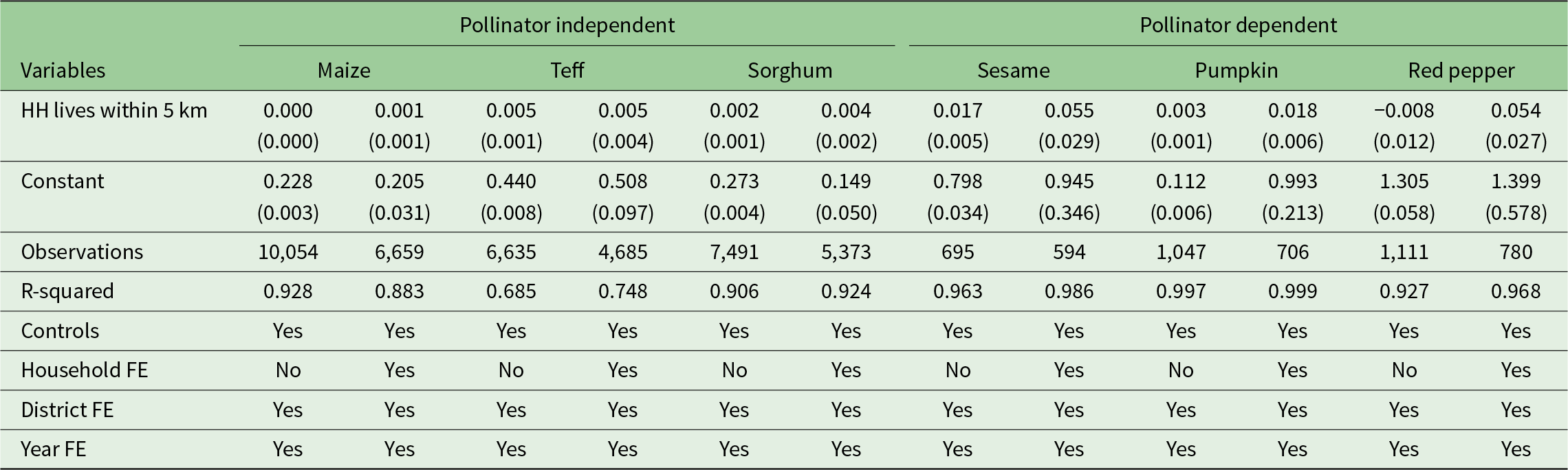
Table 8 Long description
Log unit price in US dollars per kilogram is reported for six crops, split into two groups labeled, Pollinator independent and, Pollinator dependent. Columns are Maize, Teff, Sorghum, Sesame, Pumpkin, and Red pepper, with two estimates per crop. For, HH lives within 5 km, coefficients are Maize 0.000 and 0.001, Teff 0.005 and 0.005, Sorghum 0.002 and 0.004, Sesame 0.017 and 0.055, Pumpkin 0.003 and 0.018, and Red pepper minus 0.008 and 0.054; standard errors are shown in parentheses beneath each value. Constants are Maize 0.228 and 0.205, Teff 0.440 and 0.508, Sorghum 0.273 and 0.149, Sesame 0.798 and 0.945, Pumpkin 0.112 and 0.993, and Red pepper 1.305 and 1.399, with standard errors listed below. Observations are Maize 10,054 and 6,659, Teff 6,635 and 4,685, Sorghum 7,491 and 5,373, Sesame 695 and 594, Pumpkin 1,047 and 706, and Red pepper 1,111 and 780. R squared values are Maize 0.928 and 0.883, Teff 0.685 and 0.748, Sorghum 0.906 and 0.924, Sesame 0.963 and 0.986, Pumpkin 0.997 and 0.999, and Red pepper 0.927 and 0.968. Controls are marked Yes in all columns; Household FE is No in the first column of each crop pair and Yes in the second; District FE and Year FE are Yes in all columns.
Notes: Each pair of columns reports the impact on the log unit price (US$/kg) for the indicated crop. Odd-numbered columns are the pooled OLS specification with zone and year FE estimated on all five waves; even-numbered columns add household FE on the longer (2011, 2013, 2015) sub-panel. Controls are the same as in Table 2, with the addition of the plot-level controls described in the notes for Table 7. Standard errors clustered at the household level in parentheses.
5. Conclusion
In this paper, we used five waves of nationally representative LSMS survey data from Ethiopia to estimate the economic impact of managed bees using pooled OLS. Our results reveal that households living closer to those who own managed bees experience an increase in agricultural value of about 12 per cent (about US\$120 per year). The results are generally robust to different specifications and definitions of living close to a beekeeper. We further show that the external benefits are substantial, at about a 10 per cent increase in agricultural value. We also find a non-trivial intensive margin: a 10 per cent increase in the local number of bee colonies raises gross crop revenue by roughly 0.4 per cent, and a 100 per cent increase in distance to the nearest beekeeper reduces gross crop revenue by roughly 3 per cent. A back-of-the-envelope national calculation suggests that managed bees contribute roughly US\$900 million per year (4.6 per cent of agricultural GDP) through pollination services – a substantial economic value that is largely uncounted in the official accounts and that adds to the well-documented contribution of beekeeping via honey and beeswax sales. Given the substantial positive externalities we show in this paper and the decline in wild bees, there is potential for commercialized pollination services if farmers are made aware of the role of pollinators. The connection to national-level GDP indicates the need to broaden the discussion of honeybees beyond their direct income roles. To increase the pollination benefits of beekeeping, which is primarily promoted for honey income, stakeholders will need to disseminate integrated pest and pollinator management that couples beekeeping with PD crops.
Using plot-level data, we quantified the extent to which managed bees increase the value of agricultural outputs. We find that the effect of managed bees on crop-level yield is largely inconsistent, with no clear pattern. This could be because yield is affected by many factors, and most farmers may not report it accurately. There is suggestive evidence that the effect is mostly positive for PD crops. However, we find strong and consistent evidence that living within 5 km of a beekeeper is associated with receiving higher prices for mostly PD crops. This suggests that pollination from managed bees increases the quality of horticultural produce. Future declines in wild pollinators due to land use change, climate change and increasing use of pesticides without a compensating increase in managed bees will affect agricultural production. This will have strong socioeconomic repercussions. Policymakers and development partners might need to pay attention to the role of pollinators in increasing agricultural productivity and incomes in rural areas and to fully exploit the role of managed bees for food and nutrition security.
Despite these insights from our study, there are areas for improvement that future research should address. We did not have GPS coordinates of the plots; hence, we were unable to measure the distance between EAs. Future research could measure the distance between beehives and plots to improve measurement and impact estimates. Although we controlled for a battery of control variables, including location FE, readers should interpret the coefficients with caution and avoid claiming causality.
While the LSMS data used in this study were not specifically designed to examine pollination impacts, as they lack key variables such as hive-crop proximity and contain limited crop-level yield observations, it nonetheless provides valuable national-scale insights. We used household gross revenue as the primary outcome variable, acknowledging that aggregating revenue across crops may obscure pollination’s specific contribution to crop production. Despite these limitations, the analysis provides a direct quantification of the positive externalities of beekeeping using nationally representative panel data, extending beyond small-scale experimental studies that often have limited external validity (Rollin and Garibaldi, Reference Rollin and Garibaldi2019).
Future data collection investments should therefore prioritize representation of PD crops, including sufficient observations, and systematically capture spatial information on hive–crop proximity to more accurately estimate pollination effects. We further recommend conducting randomized controlled trials in real-world farming conditions to rigorously estimate the effects of colony placement intensity and optimal beekeeping practices on crop production. Such studies could help provide insights on pollination management guidelines that consider not only beehive density but also pollination efficiency, bee health and landscape effects, among other parameters.
Supplementary material
The supplementary material for this article can be found at https://doi.org/10.1017/S1355770X26100734.
Acknowledgements
The views expressed herein do not necessarily reflect the official opinion of the donors. The authors thank Dr Mihret Getaneh Chefke for organizing the forest cover data. They also thank the editors of Environment and Development Economics and the two anonymous reviewers for their constructive comments and suggestions.
Funding statement
The authors gratefully acknowledge the financial support for this research from the Fruit Tree Agroecological-base Project (BMZ/GIZ Contract Number 81298148); the Swedish International Development Cooperation Agency (Sida); the Swiss Agency for Development and Cooperation (SDC); the Australian Centre for International Agricultural Research (ACIAR); the Government of Norway; the German Federal Ministry for Economic Cooperation and Development (BMZ); and the Government of the Republic of Kenya.
Competing interests
The authors declare none.