Implications
Despite a constant increase in the productivity of their labour, suckler beef farmers have seen zero gain in income for over 30 years now. This rise in labour productivity masks a drop in all other factors of production, ultimately culminating in only timid gains in total factor productivity (TFP) growth. The beneficiaries of these productivity gains are actors in the downstream value chain, and the drop in commodity prices is essentially backed by government money.
Introduction
Factor (labour and/or capital and/or intermediate inputs) productivity has always been seen as the main driver of economic growth (Kendrick and Sato, Reference Kendrick and Sato1963) and competitiveness (Ball et al., Reference Ball, Butault, Juan and Mora2010; Latruffe, Reference Latruffe2010). Productivity gains made by agriculture, which outstripped practically every other sector of the French economy over the last six decades, have enabled declining farm production costs and declining farm commodity prices (Charroin et al., Reference Charroin, Veysset, Devienne, Fromont, Palazon and Ferrand2012). Up until the early 1990s, agriculture made substantial productivity gains in both Europe and the United States (Ball et al., Reference Ball, Bureau, Butault and Nehring2001). French agricultural output swelled 2.2-fold in volume between 1955 and 2010, driven by specialized farms, increased use of inputs, and increased capital intensity (equipment and buildings), while the share of the working-age population in agricultural work collapsed from 31% to 3.4% (Charroin et al., Reference Charroin, Veysset, Devienne, Fromont, Palazon and Ferrand2012). Nevertheless, since the late 1990s, even though labour productivity on commercial farms continues to climb, French agriculture and the wider food-farming industry have been losing competitiveness (Butault and Réquillard, Reference Butault and Réquillard2012), as farmers struggle to hold onto their income and the productivity of all other resource factors (capital, land, intermediate inputs) is asphyxiating. Suckler beef production has counted among the sectors of agriculture most heavily subsidized by support-policy aids since the 1992 Common Agricultural Policy (CAP) reforms (Chatellier et al., Reference Chatellier, Guyomard and Le Bris2003). Beef cattle farms in France have been continually restructuring, rebuilding, readapting and improving their labour productivity, and yet beef cattle farmers continue to register less income than practically any other sector of the French agriculture economy with no real signs of improvement on the horizon (Charroin et al., Reference Charroin, Veysset, Devienne, Fromont, Palazon and Ferrand2012; Veysset et al., Reference Veysset, Benoit, Laignel, Bébin, Roulenc and Lherm2014a). Veysset et al. (Reference Veysset, Lherm, Roulenc, Troquier and Bébin2015) have demonstrated and analysed the drop in variable-factor productivity for French suckler-cattle farms over 23 years (from 1990 to 2012). The aim of this study is to measure the evolution of the partial and TFP over the past 36 years (1980–2015) for these French suckler-cattle farms, and to analyse the distribution between agents in the economy of these productivity gains. The generation and distribution of TFP gains are evaluated here by the surplus accounting method (Burlaud and Dahan, Reference Burlaud and Dahan1985; Boussemart et al., Reference Boussemart, Butault and Ojo2012).
After presenting the study sample of Charolais suckler beef farms, we start by detailing the methodology choices adopted. We then chart the macrotrends over a 36-year time series (1980–2015), by dividing this long period into three sub-periods (1980–92, 1993–2005 and 2006–15) and accounting for partial factor productivities, productivity surplus (PS) and how this surplus is redistributed between agents in the economy. We go on to discuss the macrotrends observed over three sub-periods.
Material and methods
The scholarship on productivity gain distribution addresses either a whole sector such as agriculture or a specific product sub-sector (Christensen, Reference Christensen1975; Ball et al., Reference Ball, Bureau, Nehring and Somwaru1997; Boussemart et al., Reference Boussemart, Butault and Ojo2012), and either way, it is always entirely reliant on aggregated data from national or regional agriculture-sector accounts. However, the former employment, income and costs Council of France (CERC, 1980) underlines that it is better to work on individual data rather than aggregates, as the surplus calculations are affected by aggregation biases. Data on individual businesses is rarely available, often blurred (statistical secrecy), and already part-aggregated without the technical details on farm businesses’ component commodity steams. Here we adopt a novel approach that breaks from pre-existing studies by analysing the productivity gains of a network of suckler beef farms via a bottom-up approach. Accountancy data for this livestock farm network provides detailed structural, technical and econometric data on each individual farm. The productivity gains and price advantages (PA) of the farm products and factors of production are first calculated for each individual farm and then aggregated up to analyse the long-run trend trajectories of the whole-network data set.
Data from a Charolais suckler beef farms network
In order to conduct studies on the structural, technical and economic evolutions of French beef farms, since the 1970s the French National Institute for Agricultural Research (INRA) set up a Charolais-region farm network for long-term observations (Veysset et al., Reference Veysset, Lherm, Roulenc, Troquier and Bébin2015). Each farm in the network is sample-surveyed every year. Data is collected on labour, structure, hectarage and land allocation scheme, herd, intermediate inputs, sales, aids and subsidies, investments, and borrowing. The set of technical–economic variables computed from these field surveys are geared to a technical–economic vision of farm management, which features a harmonized calculation on depreciation and depletion for each farm. As productivity gains measure year-on-year variation (see below), we filtered our database for the sub-sample of farms that had been surveyed at least two consecutive years after 1980 (the year marking the time-series with zero missing data across all farms in our survey network). Our sub-sample thus counts 164 farms between 1980 and 2015, that is, 3127 farm–year observational datapoints over the 36-year series, with a mean of 87 observations per year (the network counts a maximum of 99 farms in 1985 and 1986 and a minimum of 60 farms in 2015). Our sample is relatively stable over the long-term, with a mean farm presence-in-series of 19 years.
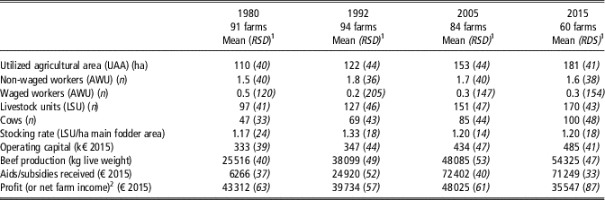
These farms are big commercial beef cattle operations (Table 1). Between 1980 and 2015, at near-constant labour units, they have expanded in hectarage (+64%) and herd size (+75%), thus doubling their meat output in the process. Operating capital (excluding land) increased by 46%. The farms in this sample all run a grass-based feed systems with relatively non-intensive main forage area (MFA) management (stocking rate at 1.17 to 1.20 livestock units (LSU)/ha MFA). Demand-side pressure (Italian market) has driven deep change in the type of cattle farmed, operating a switch from long grow-out cycles (fattened steers and heifers sold between 30 and 36 months) to young store cattle (weanling cattle sold between 10 and 12 months). These structural and productive system shifts, even coupled with huge increases in aid payments received under successive common agricultural policy (CAP) reforms, only managed to just about protect the income of livestock farmers (Veysset et al., Reference Veysset, Benoit, Laignel, Bébin, Roulenc and Lherm2014a). Both the structural trends (labour, hectarage, herd size) and economics trends (output, intermediate inputs, capital, income) observed on this INRA–Charolais-network sub-sample are wholly comparable to the trends observed on the commercial beef cattle farms in the Farm Accountancy Data Network (farming type 46 specialist cattle) statistically representative of French farm businesses (Veysset et al., Reference Veysset, Lherm, Roulenc, Troquier and Bébin2015).
Main structural and economic characteristics of the sample of Charolais suckler beef farms from the inra-network for the years 1980, 1992, 2005 and 2015

AWU=annual work units.
1 RSD=Relative standard deviation= ${{{\rm standard}\,{\rm deviation}} \over {{\rm mean}}}{\rm \,\%\,}$.
2 Profit (or net farm income)=gross farm product (including aids and subsidies)−intermediate inputs−labour costs (wages, payroll taxes and social contributions) −land rent−financial costs.
Gains in total factor productivity and surplus account
Between two fiscal years (year t and year t+1), the productivity gains measure changes in output volume net of variations in factor volumes (intermediate inputs, capital, land, labour). A variation in the partial productivity of a given factor is readily measurable, by ratioing output to that factor only (the output yield or partial productivity of one hectare of cereal crop, for instance), but this approach fails to co-account all the factors used to produce output. In contrast, the more exhaustive measure of TFP is a calculation that models the aggregate value of all product (output) variations as a function of the aggregate value of all factor (input) variations. As explained by Christensen (Reference Christensen1975), and used by Ball et al. (Reference Ball, Bureau, Nehring and Somwaru1997), the measure of the TFP of the agricultural sector (or of a farm) has to include the intermediate inputs, as well as capital and labour. If Y jt and X it are the respective amounts of output j and input i at date-point t, dY j and dX i are their corresponding variations between the two date-points t and t+1, α j is the portion of output j in total output produced and β i is the portion of input i in total volume of inputs, then we get:
 $$\eqalignno{ & {{dTFP} \over {TFP_{t} }}{\equals}\mathop \sum\limits_{j{\equals}1}^J \alpha _{j} {{dY_{j} } \over {Y_{{j,t}} }}{\minus}\mathop \sum\limits_{i{\equals}1}^I \beta _{i} {{dX_{i} } \over {X_{{i,t}} }} \cr & \quad dY_{j} {\equals}Y_{{j,t{\plus}1}} {\minus}Y_{{j,t}} \cr & \quad dX_{i} {\equals}X_{{i,t{\plus}1}} {\minus}X_{{i,t}} $$
This calculation has to proceed in two steps. The first step is to measure the volume change in each item. If the volumes of each item are unknown, they are computed from the annual mean econometric quantities observed and their specific price indexes (Diewert, Reference Diewert2003). By investigating in constant price terms, that is, by deflating the value of each income or expenditure by its respective price index, the observed year-on-year variation corresponds to the volume change of the item. Then, the second step is to weight the rate of input and output variation by the 2-year means of their respective shares in total all-output returns.
 $$\eqalignno{ & \alpha _{j} {\equals}{1 \over 2}\left( {{{p_{{j,t}} Y_{{j,t}} } \over {\mathop{\sum}\limits_{j{\equals}1}^J {p_{{j,t}} Y_{{j,t}} } }}{\plus}{{p_{{j,t{\plus}1}} Y_{{j,t{\plus}1}} } \over {\mathop{\sum}\limits_{j{\equals}1}^J {p_{{j,t{\plus}1}} Y_{{j,t{\plus}1}} } }}} \right) \cr & \beta _{i} {\equals}{1 \over 2}\left( {{{w_{{i,t}} X_{{i,t}} } \over {\mathop{\sum}\limits_{i{\equals}1}^I {w_{{i,t}} X_{{i,t}} } }}{\plus}{{w_{{i,t{\plus}1}} X_{{i,t{\plus}1}} } \over {\mathop{\sum}\limits_{i{\equals}1}^I {w_{{i,t{\plus}1}} X_{{i,t{\plus}1}} } }}} \right) \cr & p_{j} {\equals}unit\,price\,of\,product{\rm }(output){\rm }j \cr & w_{i} {\equals}unit\,price\,of\,factor(input){\rm }i $$
The surplus accounts serve to single out how the economic surplus driven by productivity gains is distributed between agents in the economy. For each fiscal year at date t, considering that total value of different outputs J totally covers the value of different inputs I (balanced general profit/loss account; a general equilibrium that corresponds to the assumption of total income entirely dissolved in paying off total factor costs), we arrive at:
 $$\mathop \sum\limits_{j{\equals}1}^J p_{{j,t}} Y_{{j,t}} {\equals}\mathop \sum\limits_{i{\equals}1}^I w_{{i,t}} X_{{i,t}} $$
Thus, between two periods t and t+1, the variation in output values will be equal to the variation in input value:
 $$\eqalignno{ & \mathop \sum\limits_{j{\equals}1}^J p_{{j,t{\plus}1}} Y_{{j,t{\plus}1}} {\minus}\mathop \sum\limits_{j{\equals}1}^J p_{{j,t}} Y_{{j,t}} {\equals}\mathop \sum\limits_{i{\equals}1}^I w_{{i,t{\plus}1}} X_{{i,t{\plus}1}} \cr & {\minus}\mathop \sum\limits_{i{\equals}1}^I w_{{i,t}} X_{{i,t}} {\rm }$$
After a re-arrangement of equation (2), it is easy to show that the period-to-period output and input value variations can be decomposed into volume and price variations.
 $$\eqalignno{ & \mathop \sum\limits_{j{\equals}1}^J p_{{j,t}} dY_{j} {\minus}\mathop \sum\limits_{i{\equals}1}^I w_{{i,t}} dX_{i} {\equals} {\minus}\mathop \sum\limits_{j{\equals}1}^J Y_{{j,t{\plus}1}} dp_{j} \cr & {\plus}\mathop \sum\limits_{i{\equals}1}^I X_{{i,t{\plus}1}} dw_{i} {\rm } \cr & \rm PS{\equals}PA$$
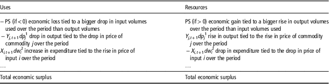
In equation (3), the left-hand side term becomes the difference, between periods t and t+1, in volume variations between outputs and inputs at the initial-period price. This value gap tied to volume variations is called PS. Productivity surplus will be positive (between two periods) when output volumes grow faster than input volumes, and negative otherwise. The right-hand side term measures the sum of the PA. For a given agent in the economy, their PA between two periods t and t+1 equals the price variations weighted by the volumes of period t+1. An input price increase is considered a PA for the input supplier (who gets paid more), while an output price decrease is considered a PA for the customer (as the output price becomes cheaper). Equation (3) expresses that PS equals sum of PA. This equality explicitly demonstrates that between two periods, a business cannot distribute as payment changes (or PA) more than it can generate from productivity gains. Net-negative PA can be considered as net provisions from stakeholders, and is cumulatable with a net-positive PS, which thus gives the total amount of resources that the beneficiaries of positive PA will share out. If the business registers a drop in productivity (PS<0), it has to counterbalance by making certain stakeholders pay more for outputs or less for inputs – and either way bear the brunt of price disadvantages, as the absolute (real) value of the PS becomes an added amount to finance. Here we can establish a uses/resources-balanced surplus account (Table 2).
Balanced economic surplus account of a holding

PS=productivity surplus.
The surplus accounts singles out how the economic surplus driven by productivity gains (quantities variations) is distributed between agents in the economy (prices variations). All the origins (Resources) of the balanced account are distributed (Uses).
1 Y j,t+1 amounts of output j at date-point t+1, dp j price variations of the output j between the two date-points t and t+1.
2 X i,t+1 amounts of input i at date-point t+1, dw i price variations of the input i between the two date-points t and t+1.
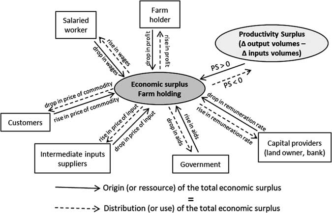
On aggregate, the price and quantity variations connect to either an ‘origin’ (resource) or a ‘distribution’ (use) of the total economic surplus, thus enabling us to analyse all the corresponding transfers (Figure 1) among customers, suppliers of intermediate inputs (feedingstuffs, fertilizers, fuels, services and so on), suppliers of primary factors (labour, land, fixed assets) and government subsidies and taxes (EU, national, regional, etc.).
Distribution of the productivity gains and price advantages. Balanced economic surplus account.

Working up from equation (1), the relative (expressed in % terms) rate of TFP growth can likewise be calculated using the surplus rate by dividing PS by the total value of output (Boussemart et al., Reference Boussemart, Butault and Ojo2012).
 $${{dTFP} \over {TFP_{t} }}{\equals}{{\mathop{\sum}\limits_{j{\equals}1}^J {p_{{j,t}} dY_{j} } {\minus}\mathop{\sum}\limits_{i{\equals}1}^I {w_{{i,t}} dX_{i} } } \over {\mathop{\sum}\limits_{j{\equals}1}^J {p_{{j,t}} Y_{{j,t}} } }}$$
In equation (3), the volume variations between periods t and t+1 were weighted by the initial-period prices (Laspeyres-type index) while the price variations were weighted by the final-period volumes (Paasche-type index). We could equally well have chosen a Paasche-type index for the volume variations and a Laspeyres-type index for the price variations. The choice of index used is not, therefore, a neutral choice. To ensure that the final result is not dependent on a random choice of index type, we use the Bennet approach which consists in computing the arithmetic mean of the Laspeyres and Paasche expressions (Caves et al., Reference Caves, Christensen and Diewert1982):
 $$\eqalign{\mathop \sum\limits_{j{\equals}1}^J \left( {{{p_{{j,t}} {\plus}p_{{j,t{\plus}1}} } \over 2}} \right)dy_{j} {\minus}\mathop \sum\limits_{i{\equals}1}^I \left( {{{w_{{i,t}} {\plus}w_{{i,t{\plus}1}} } \over 2}} \right)dx_{i} {\equals} \cr {\minus}\mathop \sum\limits_{j{\equals}1}^J \left( {{{y_{{j,t}} {\plus}y_{{j,t{\plus}1}} } \over 2}} \right)dp_{j} {\plus}\mathop \sum\limits_{i{\equals}1}^I \left( {{{x_{{i,t}} {\plus}x_{{i,t{\plus}1}} } \over 2}} \right)dw_{i} $$
Empirical modelling
For each farm in our database of suckler cattle operations, we have the real volumes (quantities) for the following outputs:
∙ beef live weight produced;
∙ sheep live weight produced;
∙ cereal crops produced.
These three outputs together account for 90% to 95% of the gross value excluding aids of total farm output. With the value and volumes of these outputs for each farm and each year, we were able to compute the year-by-year unit prices of each of these outputs, and directly dissociate the volume and price values for a compact number of inputs farm-by-farm.
The labour factor
For waged labour, the net wages and payroll taxes are the values and the number of wage-earning annual work units (AWU) is taken as the volume. Net farm income, calculated as the balance between the farm’s output returns and input expenditures (including social contributions), is considered as the profit made by the farmer, and this net income (or profit) thus corresponds to payment for non-waged labour, the volume of which is given by the number of AWU going unwaged.
The land factor
The cost of use of land is represented by land rent. To overcome the biases in system of land tenure, we considered that the all utilized agricultural area (UAA) of all the farms was under land-leasing arrangements. We thus applied a mean rental on ownership land. The volume of the ‘land’ factor is thus the UAA expressed in hectares.
The capital factor and financing costs
The capital addressed here only concerns fixed assets (farm buildings and fixed equipment, land improvements, machinery and equipment) and does not integrate the land and the herd-count. We distinguish two components of the account relating to the capital: (i) the physical capital (equipment, buildings), whose use in the production process causes equipment wear (consumption of fixed capital); this is measured by the depreciation; (ii) the immobilization in the holding of a financial capital provided by a supplier; these debts are remunerated by the interest paid. To respect the principle of the surplus accounts method, which is to assign a PA per partner identified for each entry of the farming accounts, we allocate the financial costs to the suppliers of the borrowed capital (mainly banks), and depreciation to the suppliers of equipment.
The volume (kg) of concentrate feedingstuffs purchased is known. This item accounts for 15% to 20% by value of total intermediate inputs.
As we only have the economic value for the other outputs and inputs, we use their respective prices indices to decompose the volume–price split. The index of producer prices of agricultural products (IPPAP) is designed as a metric of changes in prices paid to farmers (Eurostat, 2017). The annual values of output oilcrops, pigs and poultry for each farm in our farm network sample were deflated by their respective IPPAP.
Given the significance of aids and subsidies as important returns of livestock farm economics, the question arises as to their volume–price split. We worked to the assumption that these aids and subsidies did not change volume as they are broadly decoupled, and so price-effect of variation in subsidization thus corresponds to the observed variation in total price value. This means that we have year-to-year price movement but not year-to-year volume change.
The index of purchase prices of the means of agricultural production (IPPMAP) serves to track and trend the unit prices that farmers pay for goods and services needed for their farming activity (Eurostat, 2017). Just like for the output series, the annual mean values of each expenditure – seed, fertilizer and soil amendments, veterinary, pest control products, energy, capital goods, consultancy and overheads – of each farm in our network sample were deflated with their own respective annual IPPMAP.
All changes in volumes, prices (all nominal-value prices internalize currency depreciation using the national consumer price index as deflator), PS and PA are calculated at every year t+1 as the differential with year t for each farm present in-sample at both years t and t+1. The annual PS and PA results are averaged and then the averages are summed to get the cumulative PS and PA surplus figures, and thus establish the balanced surplus account over the period of study.
The 36-year period (1980–2015) was stratified into three sub-periods charting the major CAP reform landmarks and the year these reforms came into full force. The core of the 1992 ‘MacSharry reforms’, which were phased in from 1993, was to cut intervention prices for cereals and beef and compensate farmers through producer subsidies coupled to hectare of land and head of livestock. The 2003 ‘Luxembourg Agreement’, which came into full force in 2006, introduced the partial decoupling of subsidies and the single payment scheme. 2015 was the first year of the new 2015–20 CAP, and did not represent a significant breakdown compared to the previous rules (the new payments will be implemented progressively over the 5 years). The three sub-periods thus span: 1980–92 (13 years), 1993–2005 (13 years) and 2006–15 (10 years). The 36-year period was also marked by a record-breaking drought in 2003 that caused a collapse in fodder production, two bovine spongiform encephalopathy crises in 1996 and 2000–01, and cereal price spikes in 2007 and 2012.
Results
Partial and total factor productivity and productivity surplus
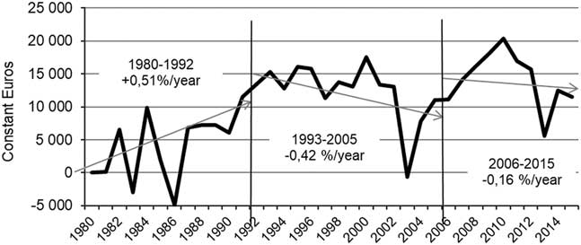
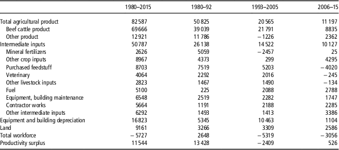
Over the 36-year period under study, mean farm area (UAA) has increased at a mean rate of 1.69% per year and volume of farm output has increased at a mean pace of 2.03% per year, whereas total labour input has remained practically unchanged, and is even tending to drop (−0.05%/year). We thus have contrasted trajectories of the partial factor productivity figures (Table 3). Labour-factor productivity has climbed steadily over the 36 years, whereas land-factor productivity has been in decline since 1992 (with an extensification of fodder area while cereal crop yields have stagnated). In global trend terms, there has been a net decline in the productivity growth of intermediate inputs. Heavy investment in buildings and equipment over the 1990s meant that farm equipment productivity plummeted between 1993 and 2005. In global trend terms, after a phase of growth from 1980–92 (+0.51%/year), TFP (or the cumulative trend in PS) shrank by 0.42%/year from 1993 to 2005 and 0.16%/year since 2006, that is, a net decline in TFP of 0.07%/year between 1993 and 2015 (Figure 2).
Productivity surplus as cumulative 1980–2015 figure and annual growth rate per sub-period for the Charolais suckler beef farms from the inra-network.

Breakdown of partial and total factor productivity, average annual growth rate of the Charolais suckler beef farms from the inra-network, in %

Surplus accounting: origin (resources) and distribution (use) of the cumulative economic surplus
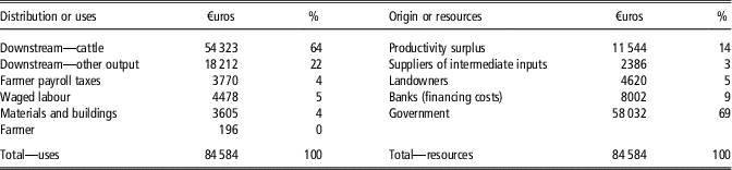
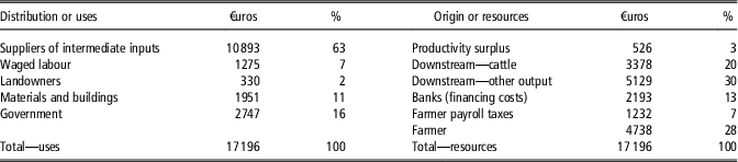
Over the end-to-end 36-year period, the cumulative surplus of TFP and absolute (real) value of negative PA, in constant-euro values and per-farm mean, comes to a total economic surplus of €84584, that is, €2350/year (Table 4). This economic surplus essentially comes from government (69%) via aid support to livestock farmers, with only 14% coming from productivity gains. In global trend terms, over the period, there has been an observable drop in intermediate input prices and land leasing prices (which account for 3% and 5%, respectively, of economic surplus). Despite some productivity gains (PS>0, Table 5) and all the government subsidies, farmer income has not moved and remains flat. 86% of these resources is captured downstream, as a drop in commodity prices. The downstream beef cattle value chain captures 64% of the resources generated. Farmers’ payroll taxes have increased despite stagnating income capturing 4% of resources, cost of waged labour has only slightly increased, and suppliers of fixed assets and equipment have captured 4% of the surplus.
Cumulative surplus account figures for the 1980–2015 period: mean distribution/uses and origin/resources in constant-euro values and % share, per Charolais suckler beef farms from the inra-network

Detail of the productivity surplus (volume effect): mean in constant-euro value cumulated over the period 1980–2015, and over the three sub-periods (1980–92, 1993–2005 and 2006–15), per Charolais suckler beef farms from the inra-network

1980–92 period: gains in productivity and strong drops in commodity prices
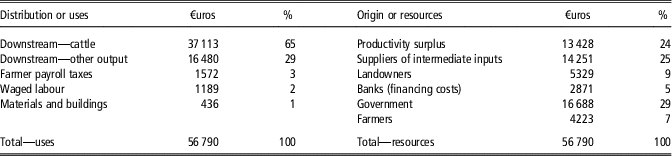
Over this 13-year period, the origin of the total economic resources (€56 790, i.e. €4368/year, Table 6) was shared between gains TFP (24%), a drop in intermediate input prices (25%), and an increase in government money (29%). A 94% majority of these resources has been captured downstream – 65% downstream of the cattle value chain as a drop in prices. The drop in intermediate input prices was essentially driven by the drop in petrol prices, which led to a drop in the cost of fertilizers, and by the drop in cost of animal feedingstuffs, which is itself linked to the drop in cereal prices. The rise in subsidization – and thus in government money – in the origin of the economic surplus is linked to the introduction, in 1980, of the suckler cow premium as a mechanism to stop suckler beef herds being converted to more lucrative dairy cow herds, at a time when the EU already registered a milk surplus. In 1987, the special premium for male animal was also brought in to encourage fattening of bulls and steers. The drop in intermediate input prices, the technical efforts of the farmers to limit the volume of inputs used (PS>0, Table 5), and the stronger government subsidization support still failed to offset the PA captured downstream, and farmer incomes fell slightly. This drop in payment for the farmers’ labour accounts for 7% of the resources in the economic surplus generated over this 13-year period.
Cumulative surplus account figures for the 1980–92 period: mean distribution/uses and origin/resources in constant-euro values and % share, per Charolais suckler beef farms from the inra-network

1993–2005: direct support-policy payments but declining total factor productivity
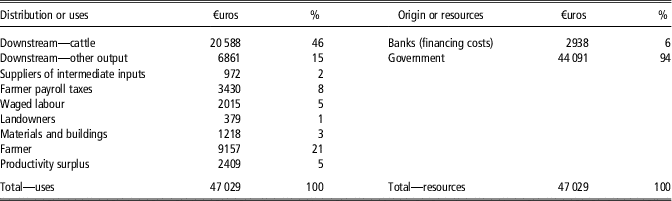
This 12-year-period’s cumulative economic resources (€47029, i.e. €3618 per year, Table 7) comes 94% from the increase in direct payments following the introduction of crop support mechanisms (cereals, high-protein oilseed and set-aside), the additional premium for extensive cattle systems (capped under a stocking-rate-per-hectare threshold), the significant revaluation of existing scheme payments (suckler cow and male premium), and, later on, the regional farmland development contracts and sustainable farming contracts. The decline in commodity cereal prices, and thus animal feedingstuff prices, continued, while market-side demand shifted towards younger and heavier animals, thus leading to a sharp increase in volume of feedingstuffs. With support policy incentivizing extensive farming systems, livestock farmers decreased their fertilizer input volumes, but at the same time investing in buildings and new fodder harvesting–storage–distribution machinery generating extra fuel-use and new needs for contract operations. In global trend terms, volume of inputs increased faster than volume of outputs (Table 5). Government money financed the entire drop in productivity, as well as the continuing drop in commodity prices and the increase in farmer incomes. These government support-policy aids, cumulated with a drop in interest rates, are distributed between the downstream sector supply chains (61%), farmers’ income and payroll taxes (21% and 8%, respectively), and the drop in TFP (5%).
Cumulative surplus account figures for the 1993–2005 period: mean distribution/uses and origin/resources in constant-euro values and % share, per Charolais suckler beef farms from the inra-network

Note that this period includes the heatwave year 2003, when the hottest summer on record led to a 50%-odd drop in grass growth. The heatwave brought about a tangible drop in quantities produced (livestock sold at lighter weight) and, crucially, an increase in animal feedingstuffs purchased. This climate episode caused a sharp decline in PS (Figure 1) and cancelled out the productivity gains made over the previous 23 years. Even if we exclude the year-2003 figures, cumulative PS over the 1993–2002 remains negative (−€345). This does not undermine the observation made above: there was effectively a real downward trend in productivity over this period, but the 2003 climate episode accentuated the trend.
2006–15 period: rise in intermediate input prices, drop in government support aids and subsidies
This period has proven the most economically stable of the three, since the annualized mean resources amount to just €1720 per year. Highlighting the period is the rise in producer price for cattle. This price rise is at the origin of 20% of the 10-year-period’s cumulative economic surplus (Table 8). The cereal price spikes in 2007 and 2012 are at the origin of 30% of the 10-year-period’s cumulative economic surplus. The rise in cereal prices, and thus animal feedingstuff prices, explains 50% of the rise in intermediate input prices, but it also prompted livestock farmers to distribute less to their animals. This declining use of purchased animal feedingstuffs, combined with the slowdown of investments in equipment and buildings, and thus a decrease in the use of capital assets, explains why PS swung back into the positive (Table 5), but it also accounts for just 3% of the origin of cumulative resources. The fact that the PS cumulated over this 10-year sub-period inched up into the positive is linked to the fact that the increase in UAA, fixed assets and intermediate inputs used is compensated for by the drop in number of AWU. However, the multi-factor (primarily labour) productivity gain and the rise in cereal crop and cattle outputs were still not enough to compensate for the rise in intermediate input prices and the scale-back of support policy (phase-out of regional farmland development contracts and ‘modulation’ of payments), all of which converged to decrease farmer income. This drop in payment for the farmers’ labour accounts for 28% of surplus-account resources.
Cumulative surplus account figures for the 2006–15 period: mean distribution/uses and origin/resources in constant-euro values and % share, per Charolais suckler beef farms from the inra-network

Discussion
The surplus accounting method, like most methods, is sensitive to the underlying assumptions. Decomposing economic value change into a volume effect and a price effect entails choices between indexes and between assumptions. Here, for instance, we chose to only consider a price effect on change in government subsidization, but as direct payments are allocated on the basis of headage or hectarage, we could equally well have chosen to consider a volume effect represented by change in number of premium-scheme cows or hectares. Calculations were repeated with this new assumption, and although the results were different in value terms, the trends of change were the same.
The bottom-up approach adopted here avoided the biases inherent to using aggregate national indexes that are not specific to a localized sector of activity. Working with real prices and volumes recorded every year for a significant set of items in the profit/loss account of each individual farm enables us to more accurately track and trend the changes in TFP established at domestic sub-sector and/or regional level.
Total factor productivity or labour productivity?
The (very timid) productivity gains over this long 36-year time-series period manage to emerge. These gains are not continuous, and they vary significantly between periods. The key highlights are continuous growth in labour productivity, stagnation in farmer income and continuous decline in technical efficiency (productivity of intermediate inputs) of the production systems. These results counter most of the results found in literature. Many studies concluded that small family-farms, at a national level, are less efficient with a lower productivity than largest specialized farms that use improved technologies and economies of scale (Gorton and Davidova, Reference Gorton and Davidova2004; Morrison Paul et al., Reference Morrison Paul, Nehring, Banker and Somwaru2004; Latruffe et al., Reference Latruffe, Balcombe, Davidova and Zawalinska2005; Mosheim and Knox Lovell, Reference Mosheim and Knox Lovell2009). However, the eco-efficiency (Keating et al., Reference Keating, Carberry, Bindraban, Asseng, Meinke and Dixon2010) of a livestock farm depends not only on its size, but also on its location or system management (Soteriades et al., Reference Soteriades, Faverdin, Moreau, Charroin, Blanchard and Stott2016). We observe capital deepening with a work-for-assets/inputs switch. The upshot is that the only real productivity gains made in beef cattle farming over the past 36 years are labour productivity gains. It is legitimate to question whether this strategy holds relevancy, if it does not benefit the worker, if it completely masks (or even holds back) the expression of technical, genetic and knowledge-capital gains.
The downstream meat value chain captures the government-financed economic surplus
The cumulative economic surplus over the 36 years under study comes 69% from government aids and goes 86% to downstream value chains, with 64% captured by the downstream beef value chain. The downstream beef value chain stretches from the first link into market (livestock commodities market, at the slaughterhouse gate) through to the consumer end, including an array of actors in the economy (livestock trader, packers and processors, caterers, distributors, and more). Thus arises the question of how this surplus is distributed throughout the value chain downstream of the farm gate. Down at the very end of the chain, the meat consumer has failed to benefit from the drop in producer prices. On aggregate, over the past 36 years, in constant-euro values, the price of cattle paid to producers slumped by 40%, whereas the price of beef paid by consumers (consumer price index for beef) climbed 20%. The pattern of change in this index thus includes a quality effect, featuring a shift towards a more services-intensive product output (mincing, marketing, packaging, food safety guarantees) (Verbeke et al., Reference Verbeke, Pérez-Cueto, de Barcellos, Krystallis and G. Grunert2010; Font-i-Furnols and Guerrero, Reference Font-i-Furnols and Guerrero2014) with all the allied costs involved, whereas back on the farm, the beef grade cattle have remained practically the same (mostly female cull cows and heifers aged 30 months-plus). France has a food pricing and profit margins observatory that monitors how prices and margins are generated throughout the farmed food supply chains and on to retail. In its latest report (FranceAgriMer, 2016), the observatory notes that beef packers and processors are still registering paper-thin pre-tax profits (0.4% to 2% of the value produced). This can be explained by the difficulties in improving raw material-to-final product conversion yields, difficulties compounded by the fact that yield gains cannot offset the tougher new environmental and food safety standards. The drop in producer price for cattle has thus been diluted through the downstream supply chain.
Government has been the main driver behind of these changes. Prior to the 1992 MacSharry reforms, the indirect support-policy payments including in commodity selling prices did not prevent productivity gains generated by farmers getting transferred downstream the beef cattle value chain. Then, over the period during which policy aids were coupled to headage and hectarage, livestock farmers were able to benefit from upvaluation through the heavy aid-scheme premiums whereas the downstream supply chain continued to profit from declining prices. Lastly, since 2006, livestock farmers have not benefited from the (partial) decoupling and modulation of support payments. By modelling, Ash et al. (Reference Ash, Hunt, McDonald, Scanlan, Bell, Cowley, Watson, McIvor and MacLeod2015) observed a positive impact of the factor productivity on beef farm profitability, but, in other hand, CAP subsidies could affect negatively the farm productivity (Rizov et al., Reference Rizov, Pokrivcak and Ciaian2013). Bojnec and Latruffe (Reference Bojnec and Latruffe2013) observed that medium-size farms in Slovenia are the less profitable: large farms are technically efficient and small farms are highly subsidized and more allocatively efficient. Ultimately, French beef farmers’ income is not correlated to farmer productivity gains, and government subsidies do not always benefit the professional branch they are partly intended for. Government subsidies to farming are designed to support a number of objectives (to support farming income, to support price-competitive agrifood supply chains, to curb food price inflation, etc.), yet in the case of the beef sector, producers have captured practically none of this support.
The constant increase in the farms and herds’ size, encouraged by the non-capped subsidies, led to an increase in inputs and equipment used per unit of output. Thus, we observed an increase in the use of fossil-fuel energy and in greenhouse gas (GHG) emissions per kilogram live weight produced, and a negative correlation between the size of these Charolais suckler-cattle farms and these environmental performances (Veysset et al., Reference Veysset, Lherm, Bébin, Roulenc and Benoit2014b). It also appeared that, through better technical performances and lower use of inputs, the less-GHG-emitting farms (that are smaller than the most-GHG-emitting farms) generated higher income per worker while consuming less fossil energy. The enlargement strategy runs counter to the clean energy challenge and the project of agroecology transition for green growth.
Conclusion
Analysis of how the Charolais beef cattle sector’s productive resources have been redistributed over the course of the past 36 years finds that the sector’s downstream customers have come out as the main winners via declining prices,. These declining prices have essentially been subsidized by government via CAP payments and other support-policy aids. There are TFP gains, but they tend to be modest, fluctuating between periods but tending to a downward curve, whereas the labour productivity of the livestock farmers shows constant steady growth. The gains in labour productivity made by the farmers mask the steady decline in all other factor productivity (land, intermediate inputs and equipment) leaving the beef cattle production systems increasingly inputs- and capital-dependent. The simple fact that farmers struggle to protect their income is a clear indication that they have been losers in this distribution of productivity gains. The strategy of continually re-adapting farm structure (up-scaling size and down-sizing labour, development of associative organization structures, investment in new infrastructure and new technologies) and farm systems (standardization of farmed animal output and feed management practices) to meet market requirements (basic commodity raw material) has not proven an entirely winning strategy for the farmers themselves. These macrotrends manifestly mask relatively significant inter-farm and year-on-year variabilities that warrant further investigation in future studies.
Livestock is more than just a sector of the economy producing market goods – it also plays a pivotal role in territorial land occupancy and rural development in less-favoured pasture-based zones where few if any viable alternatives exist. To stem the decline in value-added created by livestock farming and improve livestock farmer profits (without redistributing their share down to other agents in the economy), one solution could be to more actively couple farm outputs to territory, via localized bioregional farming practices (fattening livestock locally) and quality labels. In a context of beef consumption declining, consumers express preference and willingness to pay for country‐of‐origin‐labelled beef and food safety enhancements. The challenge is for livestock farmers to capture a share of the fast-growing services value component of food consumption, for example, through new marketing chains or cooperatives. Public policies, and especially the laws, could have a role by inciting the bovine sector stakeholders to establish fair agreements.
Acknowledgements
The authors thank the farmers who kindly provided the yearly data from their registers to complete this study.
Declaration of interest
The authors declare no competiting interests regarding this publication.
Ethics statement
Section is irrelevant for this study.
Software and data repository resources
Data used are individual economic data protected by statistical confidentiality. They were not deposited in an official repository.