2.1 Vibration-based fault diagnosis in rotating machinery

Vibration analysis for rotating machinery is a mature field. The tutorial by Randall and Antoni on rolling-element bearing diagnostics remains a standard reference for the underlying signal processing [Reference Randall and Antoni13]. The same principles, including envelope analysis, cyclostationary modelling and order tracking, transfer reasonably well to propeller analysis once a speed reference is available. Reviews by Liu et al. [Reference Liu, Yang, Zio and Chen14] and Lei et al. [Reference Lei, Yang, Jiang, Jia, Li and Nandi15] document how the field has absorbed machine learning over the past decade. Sharma and Parey provide a more focused account of condition indicators in gear diagnosis [Reference Sharma and Parey16]. A complementary strand of the literature concerns the wireless side of the problem, and the trade-offs typically identified for industrial wireless monitoring (battery life, packet loss and sampling-rate limits imposed by the radio link) extend almost directly to the small-UAV use case considered here.

Rangel-Magdaleno et al. employed discrete wavelet decomposition to detect partially damaged rotor bars in induction motors under varying load [Reference Rangel-Magdaleno, Peregrina-Barreto, Ramirez-Cortes and Cruz-Vega17]. Although their setup is industrial rather than airborne, the central finding, that mid-band wavelet energies separate healthy from faulty conditions more cleanly than raw time-domain statistics, motivates the choice of statistical descriptors used in the present study. Simple moments were preferred over wavelet coefficients because the sampling rate available over the Wi-Fi link is too low to resolve high-frequency content.

2.2 Acoustic and IMU-based UAV propeller monitoring

Two complementary modalities have been investigated for small UAVs. Acoustic monitoring is attractive because it does not require an airframe-mounted sensor. Iannace et al. trained a neural network on microphone recordings of healthy and damaged quadrotor blades [Reference Iannace, Ciaburro and Trematerra18]. Altinors et al. later extended this approach to UAV motors using hand-crafted spectral features and reported high accuracy in a controlled acoustic environment [Reference Altinors, Yol and Yaman19]. The principal drawback is environmental: wind, ambient traffic and operator speech rapidly degrade microphone data in field conditions.

Inertial measurement unit (IMU) and accelerometer-based monitoring avoids this problem at the cost of additional payload. Bondyra et al. used the existing flight-controller IMU together with threshold-based rules to flag propeller damage [Reference Bondyra, Gardecki, Gasior and Giernacki20]. Ghalamchi et al. developed a real-time vibration-based scheme for multicopters and reported convincing detection of imbalance [Reference Ghalamchi, Jia and Mueller7]. Khalastchi et al. approached the broader anomaly-detection problem online using model-based residuals across heterogeneous sensors [Reference Khalastchi, Kalech, Kaminka and Lin21]. The work reported here belongs to the airframe-mounted tradition. It differs in that the sensor is a dedicated, externally clocked unit streaming through its own radio link, which decouples it from flight-controller bandwidth limits and from the firmware schedule of the autopilot.

2.3 Machine learning approaches for rotorcraft health monitoring

The machine-learning literature on rotorcraft health divides broadly into classical and deep approaches. On the classical side, ensemble trees, support vector machines (SVM), and $k$ -nearest neighbors (kNN) have been used for decades in bearing and gear fault classification [Reference Breiman22–Reference Quinlan25]. The original decision-tree (DT) formulation by Quinlan still underpins many of the interpretable pipelines used in industrial CBM [Reference Quinlan25]. On the deep side, Saufi et al. [Reference Saufi, Ahmad, Leong and Lim10], Zhao et al. [Reference Zhao, Yan, Chen, Mao, Wang and Gao11] and Khan and Yairi [Reference Khan and Yairi12] survey the rapid adoption of convolutional neural networks (CNNs), long short-term memory (LSTM) networks and autoencoders for vibration data. Within aerospace specifically, recurrent architectures have been applied to mini-UAV navigation-phase flight-data estimation within a Cross-Industry Standard Process for Data Mining (CRISP-DM) workflow [Reference Konar, Özdemir, Fenerci and Erşen26], hybrid artificial neural network (ANN) approaches combined with population-based optimisation have been used for emission tuning of gas turbines [Reference Konar, Cam and Aktaş27], and supervised regression has been used for aircraft takeoff-speed prediction from flight-parameter data [Reference Karaburun, Hatipoğlu and Konar28]. A complementary observation from outside the aerospace domain is that systematic benchmarking of several classical classifiers on a single labelled dataset (as performed for earthquake-induced soil liquefaction classification using RF, SVM, kNN and gradient-boosted variants) consistently identifies ensemble trees as the most stable performer under modest sample size [Reference Korkmaz Can, Ozkat, Ceryan and Ceryan29], which is one of the motivations for the model selection adopted in the present study.

For small UAVs specifically, Pourpanah et al. explored hybrid feature-selection schemes positioned between classical and deep regimes [Reference Pourpanah, Lim, Wang, Tan, Seera and Shi30], and Wang et al. applied a hybrid prognostics scheme for bearings [Reference Wang, Lei, Li and Li31]. A recurring observation across these studies is that deep models reach strong accuracy when several thousand labelled windows are available, but degrade or fail to converge when the training set is on the order of one or two hundred windows. The classical pipeline considered here is positioned for the latter regime, which is the regime that an individual operator with a single test cell typically inhabits.

The present contribution differs from this body of work in several respects. The methodology deliberately remains within the classical regime because most recent UAV propeller-fault studies train deep models on data volumes that an operator cannot reasonably collect during commissioning, whereas the aim here is to characterise what a small operator can accomplish with one afternoon of test flights and a laptop. The flight protocol is structured around three consecutive phases (hovering, controlled manoeuvring and harsh manoeuvring), which allows phase-dependent behaviour to be quantified rather than averaged out. Both the binary and the multi-class versions of the classification problem are reported on the same dataset, which makes the performance gap between the two tasks directly visible.

To position the present study against representative prior UAV propeller and rotor fault-detection work, Table 1 summarises the sensing modality, the effective acquisition rate, the number of conditions and the test environment for each. A direct head-to-head accuracy comparison is deliberately avoided because each study uses a different platform, defect set, and dataset; the table is intended to clarify the methodological niche occupied by the present work rather than to rank accuracy. Within this landscape, the present study is distinguished by a dedicated, externally clocked accelerometer streaming over its own wireless link and by the joint reporting of binary and seven-class results on a single dataset.

Table 1.

Positioning of the present study against representative UAV propeller/rotor fault-detection work. Accuracies are not listed because they are not directly comparable across different platforms, defect sets and datasets

Table 1. Long description

Table 1: The table compares five studies across four attributes: sensing method, acquisition rate, number of classes and test environment. Iannace et al.: acoustic microphone, audio rate, 2 classes, controlled laboratory. Altinors et al.: acoustic microphone, audio rate, multiple classes, controlled acoustic environment. Ghalamchi et al.: on-board inertial measurement unit, high rate, 2 imbalance classes, indoor. Bondyra et al.: on-board inertial measurement unit with threshold rules, high rate, 2 classes, laboratory. Present work: dedicated MEMS accelerometer over a Wi-Fi link at about 10 hertz, 2 and 7 classes, indoor with no wind. Accuracies are not compared because platforms, defect sets and datasets differ.

3.1 Hardware and test platform

The test platform is a small custom-built quadrotor with brushless DC motors and four fixed-pitch polymer propellers of 19 cm diameter. The take-off mass with sensor payload is approximately 1.2 kg. The motors are driven through electronic speed controllers, and a multi-cell lithium-polymer battery powers the platform. The autopilot is a standard hobby-grade flight controller operating in stabilised mode; it is not part of the data pipeline, and no autopilot logs are used in the present study.

The vibration sensor is an ADXL345 (analog devices), a three-axis MEMS digital accelerometer with selectable measurement range of $\pm 2$ , $\pm 4$ , $\pm 8$ or $\pm 16$ g and 13-bit resolution on each axis. For reference, the $\pm 16$ g full-scale option corresponds to approximately $\pm 157$ m/s $^{2}$ ; all accelerations in this paper are reported in m/s $^{2}$ . It communicates with an ESP32 microcontroller over an inter-integrated circuit (I $^{2}$ C) bus. The ESP32 streams the readings to a ground-station laptop over a Wi-Fi link. Figure 1 shows the transmitter unit; Figure 2 shows the healthy reference propeller with the sensor installed.

In principle the ADXL345 can sample at up to 3,200 Hz. In practice, with the Wi-Fi link included in the pipeline, the usable end-to-end sampling rate is approximately 10 Hz. This rate is a hard constraint of the wireless telemetry pipeline and precludes frequency-domain analysis of bearing or blade-pass harmonics, which lie well above 10 Hz on a multirotor of this scale. It does not, however, preclude the lower-band amplitude statistics adopted in the present study. The structural defect modes targeted here (static imbalance, leading-edge chips, asymmetric blade thinning) excite once-per-revolution and other low-order amplitude modulations that are aliased into the band below 10 Hz but remain visible as changes in the time-domain amplitude distribution: standard deviation, peak-to-peak (P2P) amplitude, root mean square (RMS) and the higher statistical moments are sensitive to these modulations even when the carrier harmonic itself is unresolved. Tables 4 and 9 confirm that this is the case in practice on the dataset considered, with healthy and high-amplitude fault classes already separable on the Y-axis amplitude statistics alone. It must be emphasised, however, that because the carrier harmonic is unresolved at this rate, the retained features capture aliased low-order amplitude modulations and may also incorporate low-frequency rigid-body airframe motion; the present results therefore establish detectability on the amplitude envelope rather than on resolved spectral lines, and the term ‘vibration monitoring’ should be read in this restricted sense. A short high-rate capture (onboard logging at the full ADXL345 bandwidth) for a healthy and a faulty case is planned to confirm that the 10 Hz amplitude statistics track the true broadband vibration energy.

Figure 1.

ESP32-based wireless sensor transmitter with ADXL345 accelerometer, mounted on the UAV airframe close to the propeller attachment point.

Figure 2.

Healthy reference propeller with the ADXL345 sensor and ESP32 transmitter installed.

Figure 3.

Examples of the deliberately damaged propellers used in the campaign, illustrating the range of mass-perturbation and surface-modification defects introduced on the blades.

Figure 3. Long description

Figure 3: Four close-up photographs of three-blade quadrotor propellers, each carrying a deliberately introduced defect. The panels show, respectively: a subtle blade-surface modification (Fault-1); a small single-blade tip-mass addition (Fault-2); an asymmetric mid-blade mass addition (Fault-4); and a symmetric tip-mass addition applied to all blades (Fault-5). The added masses are small patches placed at known positions on the blades to create a calibrated, reversible imbalance.

The sensor block is mounted on the airframe close to one of the motor mounts, at an approximate distance of 4–5 cm from the propeller hub. This motor-mount position is a deliberate departure from the more common centre-of-gravity placement used in airframe-wide health monitoring. A centre-of-gravity sensor captures the structural propagation of vibrations averaged across all four rotors, which is appropriate for global airframe diagnostics. A motor-mount sensor, by contrast, preferentially captures the signature of the rotor closest to it, which is appropriate when the question of interest is whether one specific propeller is degraded. Since the present study targets single-propeller fault identification rather than global airframe health, the motor-mount position was preferred. The ESP32 is powered by an auxiliary USB power bank carried on the airframe, separate from the main flight battery, so that no current from the propulsion bus passes through the sensing electronics.

Table 2.

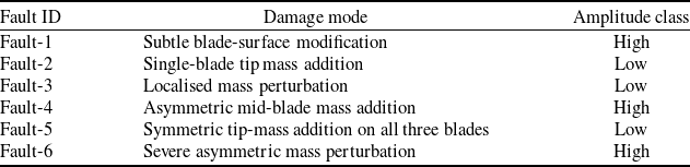
Mapping of fault identifiers to the vibration-amplitude class observed on the cleaned accelerometer record

Table 2. Long description

Table 2: The table lists each fault with its damage mode and amplitude class. Fault-1: subtle blade-surface modification, high amplitude. Fault-2: single-blade tip-mass addition, low amplitude. Fault-3: localised mass perturbation, low amplitude. Fault-4: asymmetric mid-blade mass addition, high amplitude. Fault-5: symmetric tip-mass addition on all three blades, low amplitude. Fault-6: severe asymmetric mass perturbation, high amplitude.

3.2 Propeller configurations

Seven propellers were tested: one healthy reference and six damaged propellers. The damage modes were introduced by applying controlled mass-perturbation patches at known positions along the propeller blades, which is a standard reversible surrogate technique for producing a calibrated imbalance that mimics in-service effects such as foreign-object adhesion, debris bonding and partial blade-surface modification. Representative photographs are shown in Figure 3. The modifications span single-blade tip-mass additions, asymmetric mid-blade perturbations and symmetric tip-mass additions distributed across all three blades; together they cover a range of imbalance configurations from highly asymmetric (causing strong once-per-revolution excitation) to nearly symmetric (causing primarily a global mass change with weak amplitude growth).

Defects are referred to throughout as Fault-1 to Fault-6. Table 2 maps each fault identifier to its damage mode and to the empirical vibration-amplitude class observed in the data (Tables 3 and 4).

A useful first observation, available before any classifier is trained, is that the six defects fall into two empirically distinct groups in the raw vibration record (see Tables 3 and 4; Figures 4 and 5). Fault-1, Fault-4 and Fault-6 produce high-amplitude, broad-distribution vibration signatures consistent with strongly asymmetric mass perturbations. Fault-2, Fault-3 and Fault-5 produce low-amplitude signatures whose statistics overlap with the healthy reference, consistent with localised or nearly symmetric perturbations that do not strongly excite the once-per-revolution component. This severity-based grouping is referred to in the discussion of the multi-class confusion matrix, where most of the residual error of the seven-class classifier occurs within the low-amplitude group.

3.3 Flight protocol

Each flight followed the same 180 s protocol. The first 60 s consists of steady hovering at a fixed altitude. The middle 60 s consists of controlled manoeuvring with gentle yaw, pitch, and translation inputs. The final 60 s consists of harsh flight, with deliberately aggressive stick inputs and rapid reversals. The same test pilot performed every run. The test cell is a netted indoor volume with no wind, which removes a major source of confounding low-frequency vibration.

The three phases were selected because they place qualitatively different mechanical demands on the rotor. Hovering is closest to a textbook steady state and provides the cleanest fault signature. Manoeuvring introduces controlled changes in rotor rotational speed and thrust vector. Harsh flight stresses the blade with rapid commanded accelerations and recovers some of the worst-case vibration encountered in real operational use.

Two of the runs produced shorter usable records than the nominal 180 s protocol: 42.86 s for Fault-2 and 61.44 s for Fault-3. The partial data were retained for analysis.

3.4 Preprocessing

The raw stream contains two artefacts that need to be removed before feature extraction: a sensor warm-up transient at the start of each file, and occasional spurious outliers from telemetry hiccups. An interquartile-range (IQR) rule is applied on each axis independently.

For each axis $a \in \{X, Y, Z\}$ ,

(1) \begin{equation} {\rm IQR}_a = Q_{3,a} - Q_{1,a}, \end{equation}

and a sample $x_a$ is retained only when

(2) \begin{equation} Q_{1,a} - k\, {\rm IQR}_a \;\le \; x_a \;\le \; Q_{3,a} + k\, {\rm IQR}_a, \end{equation}

for all three axes simultaneously. The multiplier was set to $k = 2.0$ . With $k = 1.5$ (Tukey’s default) an excessive proportion of high-amplitude harsh-flight samples were discarded. With $k = 3.0$ obvious spike artefacts were preserved. The value of 2.0 represents a compromise and could be tuned per flight, but it was kept fixed across the dataset for reproducibility. It should be noted that the largest removal fraction occurs for Fault-3 (33.45%), one of the low-amplitude classes; the IQR rule may therefore attenuate some genuine harsh-flight transients, and the residual misclassification of the low-amplitude group should be read with this in mind. A sensitivity analysis of the final classification accuracies to $k \in \{1.5, 2.0, 3.0\}$ is planned for the extended dataset to confirm that the reported results are not an artefact of the chosen multiplier.

Table 3.

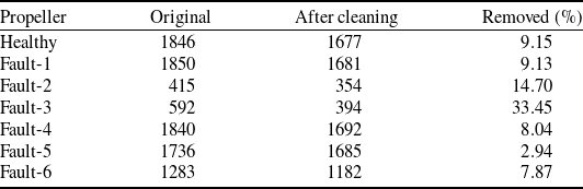
Data preprocessing summary. Sample counts per propeller before and after IQR-based outlier removal

Table 3. Long description

Table 3: For each propeller the table gives the original sample count, the count after cleaning and the percentage removed. Healthy: 1846 to 1677, 9.15 percent. Fault-1: 1850 to 1681, 9.13 percent. Fault-2: 415 to 354, 14.70 percent. Fault-3: 592 to 394, 33.45 percent. Fault-4: 1840 to 1692, 8.04 percent. Fault-5: 1736 to 1685, 2.94 percent. Fault-6: 1283 to 1182, 7.87 percent. Fault-3 has by far the largest removal fraction.

After outlier removal, each flight was clipped to the 0–180 s window so that all conditions cover the same nominal interval. Table 3 summarises sample counts before and after cleaning. The removal fraction is small (below 10%) for most flights and large (33%) for Fault-3, which had the noisiest stream.

The accelerometer signals were not explicitly gravity-compensated. The static gravity vector and any fixed mounting-angle offset appear only in the per-axis mean; the feature-importance analysis (section 4.3) shows that the three axis means carry negligible discriminative weight (each below 0.008), and the amplitude-dispersion features on which the classifiers rely (standard deviation, RMS, peak-to-peak amplitude) are by construction invariant to a constant offset. Because the sensor was mounted once and its orientation was held fixed across every propeller condition, any mounting-angle difference is common-mode and does not confound the between-condition comparison; the sensor was not removed or repositioned between runs.

3.5 Statistical characterisation

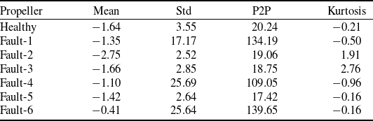
Table 4 reports summary statistics for the Y-axis, which is the axis carrying the strongest fault signature in the present configuration. The healthy propeller exhibits the lowest standard deviation, approximately 3.55 m/s $^{2}$ . Fault-1, Fault-4 and Fault-6 are markedly different, with standard deviations between 17 and 26 m/s $^{2}$ and peak-to-peak amplitudes exceeding 100 m/s $^{2}$ . Fault-2, Fault-3 and Fault-5 sit much closer to the healthy condition in raw amplitude. However, Fault-2 and Fault-3 show positive kurtosis (1.91 and 2.76), indicating heavier-than-Gaussian tails. This heavy-tailed character is the foothold that a classifier requires for these subtler defects.

3.6 Feature extraction

Features were computed on 10 s sliding windows with 5 s overlap. The 10 s length was selected as a compromise between three competing requirements: the window must contain enough samples (approximately 100 at the effective 10 Hz rate) for the higher statistical moments to stabilise; it must be short enough that no more than one of the three flight phases (hovering, controlled manoeuvring, harsh manoeuvring) is captured per window, which would otherwise blur the phase-dependent signature; and it must permit a sufficient number of windows per flight to support training, given that the nominal flight duration is 180 s and that two of the faulty-propeller runs produced shorter usable records. The 5 s overlap (50%) doubles the number of windows per flight; the resulting correlation between temporally adjacent feature vectors and its consequence for the train/test split is addressed in section 5.6. A formal sensitivity sweep of the window length (for example, 5 s, 10 s and 15 s) is left for future work. For each axis, eight statistics were computed: mean, standard deviation, RMS, P2P amplitude, skewness, kurtosis, minimum and maximum. The magnitude signal $M = \sqrt {x_X^2 + x_Y^2 + x_Z^2}$ contributes three further descriptors (mean, standard deviation and RMS). This magnitude is formed from the per-axis samples after IQR outlier removal, so its descriptors inherit the same cleaning as the per-axis features. This yields $8 \times 3 + 3 = 27$ features per window.

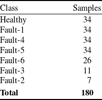
Across all seven propellers, the sliding window produces 180 feature vectors in total. The class distribution is uneven (Table 5). The four longest-running conditions – Healthy, Fault-1, Fault-4 and Fault-5 – each contribute 34 windows. Fault-6 contributes 26. Fault-3 and Fault-2 contribute only 11 and 7 windows, respectively, owing to their shorter usable records. The implications of this imbalance are revisited in the discussion.

Table 4.

Statistical summary of cleaned accelerometer data on the Y-axis. Units: m/s $^{2}$ , except kurtosis (dimensionless)

Table 4. Long description

Table 4: The table reports Y-axis statistics in metres per second squared, except dimensionless kurtosis, as mean, standard deviation, peak-to-peak, kurtosis. Healthy: -1.64, 3.55, 20.24, -0.21. Fault-1: -1.35, 17.17, 134.19, -0.50. Fault-2: -2.75, 2.52, 19.06, 1.91. Fault-3: -1.66, 2.85, 18.75, 2.76. Fault-4: -1.10, 25.69, 109.05, -0.96. Fault-5: -1.42, 2.64, 17.42, -0.16. Fault-6: -0.41, 25.64, 139.65, -0.16. The high-amplitude faults have much larger standard deviation and peak-to-peak values; Fault-2 and Fault-3 show elevated positive kurtosis.

Table 5.

Feature-vector class distribution after windowing

Table 5. Long description

Table 5: After sliding-window feature extraction the class counts are: Healthy 34, Fault-1 34, Fault-4 34, Fault-5 34, Fault-6 26, Fault-3 11 and Fault-2 7, giving 180 windows in total. The dataset is imbalanced, with two minority classes, Fault-2 and Fault-3, holding fewer than 15 windows each.

Four classical machine learning classifiers were evaluated: RF [Reference Breiman22], SVM [Reference Cortes and Vapnik23], kNN [Reference Cover and Hart24] and DT [Reference Quinlan25]. The RF model used 100 trees with bootstrap sampling and feature subsampling at each split, and final predictions were obtained by majority voting. The SVM model used a radial basis function (RBF) kernel. The kNN classifier was applied with k = 5 using the standardised feature space. The DT classifier used information-gain-based splitting.

Before training, all features were standardised using z-score normalisation. To avoid data leakage, the scaling parameters were fitted only on the training partition and then applied to the test partition. For cross-validation, standardisation was refitted separately within each training fold. The dataset was divided into training and test sets using a stratified 70/30 split. In addition, five-fold stratified cross-validation (CV) was performed on the full dataset to check whether the held-out test result depended on a particular random split. Since each propeller condition corresponds to a single continuous flight, neither the random split nor the stratified folds enforce flight-level grouping. The implications of this limitation are discussed explicitly in section 5.6.

4.1 Time-domain behaviour

Figure 4 shows representative time series for all conditions across the three flight phases. The healthy trace is the quietest. Fault-1, Fault-4 and Fault-6 visibly diverge from it within the first few seconds of hovering. Fault-2, Fault-3 and Fault-5 are not apparent by visual inspection of the raw trace, although subtle differences emerge once moments are computed.

Figure 5 shows the per-axis distributions after outlier removal. The Y-axis carries the strongest signal across most defects. This is consistent with the sensor mounting orientation, which aligns the Y-axis approximately with the dominant in-plane oscillation direction at the motor mount.

Figure 5.

Box-plot distributions of acceleration per propeller for the X, Y and Z axes after outlier removal. The box marks the interquartile range with the median line, the whiskers extend to 1.5 times the IQR, and points beyond are shown individually.

Figure 5. Long description

Figure 5: Box plots comparing the per-axis acceleration distributions of the healthy propeller and the six faults, grouped by the X, Y and Z axes. Each box marks the interquartile range with a median line; whiskers extend to 1.5 times the interquartile range and outliers are plotted individually. The Y axis shows the widest spread and the clearest separation between conditions. The healthy propeller and the low-amplitude faults (Fault-2, Fault-3, Fault-5) have narrow boxes close to zero, whereas the high-amplitude faults (Fault-1, Fault-4, Fault-6) have much wider boxes, indicating larger vibration amplitude.

Figure 6 compares vibration magnitude RMS across the three flight phases. As expected, the harsh-flight phase is louder than hovering for every propeller. Notably, the contrast between healthy and faulty is largest in the hovering phase. In this phase the airframe is closest to a steady state and the fault-induced signal is not masked by manoeuvring-induced dynamics. For an in-flight monitoring scheme this is a favourable observation: the cleanest signal is available precisely during the steady periods, which is also when a control system can most readily take action.

Figure 6.

Vibration magnitude (RMS) across flight phases for each propeller condition.

Figure 6. Long description

Figure 6: A grouped bar chart showing root-mean-square vibration magnitude for the healthy propeller and the six faults, with three bars per condition for the hovering, manoeuvring and harsh-flight phases. For every propeller the harsh-flight bar is the tallest and hovering the shortest. The gap in RMS between the healthy propeller and the high-amplitude faults is largest during the hovering phase, where the fault signature is least masked by manoeuvring dynamics, and smaller during harsh flight.

4.2 Multi-class classification

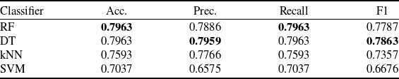
Table 6 reports the seven-class results on the held-out test set. RF reaches 79.63% accuracy and an F1 of 77.87%. DT matches the same accuracy with a marginally higher F1 of 78.63%, while kNN and SVM trail at 75.93% and 70.37%, respectively. The confusion matrix in Figure 7 explains the origin of the errors. They concentrate among Fault-2, Fault-3 and Fault-5, the three low-amplitude faults whose univariate moments are similar to the healthy baseline. The high-amplitude faults (Fault-1, Fault-4, Fault-6) are almost never confused with each other or with the healthy class. On this seven-class task, the difference between RF and DT lies within the resolution of a 54-sample test set: the two share an identical accuracy of 79.63%, and DT is in fact marginally ahead on F1. They should therefore be regarded as statistically comparable here, and the clear separation of RF from the field is established on the binary task and under cross-validation (Table 9) rather than on this single multi-class split. A formal pairwise comparison (for example McNemar’s test, with bootstrap confidence intervals on the test metrics) is planned once additional flights enlarge the test set.

Table 6.

Multi-class classification results (7 classes) on the held-out 30% test set

Table 6. Long description

Table 6: The table gives accuracy, precision, recall and F1 for four classifiers on the seven-class task. Random Forest: 0.7963, 0.7886, 0.7963, 0.7787. Decision Tree: 0.7963, 0.7959, 0.7963, 0.7863. kNN: 0.7593, 0.7766, 0.7593, 0.7357. SVM: 0.7037, 0.6575, 0.7037, 0.6676. Random Forest and Decision Tree share the highest accuracy; Decision Tree has a marginally higher F1.

Note: Bold values indicate the best result in each column.

Figure 7.

Confusion matrix for the RF classifier on the seven-class task.

Figure 7. Long description

Figure 7: A seven-by-seven confusion matrix for the Random Forest classifier, with true propeller classes on the rows and predicted classes on the columns. The healthy class and the high-amplitude faults Fault-1, Fault-4 and Fault-6 lie almost entirely on the diagonal, indicating correct classification. Most off-diagonal errors fall among the low-amplitude faults Fault-2, Fault-3 and Fault-5, which are confused with one another and with the healthy class. Fault-2, with only two test windows, is never correctly predicted.

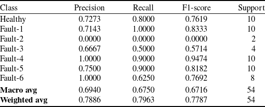
To support a class-level reading of the confusion matrix, Table 7 reports the per-class precision, recall and F1-score of the RF classifier on the seven-class task.

Table 7.

Per-class precision, recall and F1-score of the RF classifier on the 7-class held-out test set (54 trials in total)

Table 7. Long description

Table 7: For the Random Forest classifier the per-class precision, recall, F1 and support are: Healthy 0.7273, 0.8000, 0.7619, support 10. Fault-1 0.7143, 1.0000, 0.8333, 10. Fault-2 0.0000, 0.0000, 0.0000, 2. Fault-3 0.6667, 0.5000, 0.5714, 4. Fault-4 1.0000, 0.9000, 0.9474, 10. Fault-5 0.7500, 0.9000, 0.8182, 10. Fault-6 1.0000, 0.6250, 0.7692, 8. Macro average 0.6940, 0.6750, 0.6716; weighted average 0.7886, 0.7963, 0.7787; total support 54. Fault-2 is never recovered.

Figure 8.

RF Gini-based feature importance on the seven-class task, top 15 of 27 features. Amplitude-dispersion descriptors (RMS, standard deviation, P2P amplitude) dominate; the means of the three axes carry negligible weight.

Figure 8. Long description

Figure 8: A horizontal bar chart ranking the 15 most important of 27 features by mean decrease in Gini impurity. The highest-ranked features are Y-axis RMS (0.084), Z-axis minimum (0.081), Y-axis standard deviation (0.078), X-axis standard deviation (0.069) and Y-axis peak-to-peak amplitude (0.064), followed by vibration-magnitude RMS (0.054) and X-axis RMS (0.052). Amplitude-dispersion features dominate. Skewness and kurtosis rank in the lower half, none exceeding 0.020, and the three axis means carry negligible weight, each below 0.008.

The class-wise breakdown confirms the pattern already visible in the confusion matrix. The Healthy class and the three high-amplitude faults (Fault-1, Fault-4, Fault-6) are recovered with strong precision and recall, with Fault-4 reaching perfect precision at 90% recall and Fault-1 reaching perfect recall at 71% precision. The three low-amplitude faults drive almost all of the residual error of the seven-class classifier: Fault-3 is recovered at 67% precision and 50% recall, and Fault-2 is not recovered at all (precision and recall both zero on the test split). The Fault-2 collapse is principally a sample-size artefact: only seven windows of Fault-2 exist in the entire dataset, of which two end up in the test set, and an ensemble of DTs trained on the remaining five minority-class samples produces no decision path that reaches Fault-2 with majority vote at inference time. Macro-averaged F1 of 67.16% (versus weighted F1 of 77.87%) therefore overstates the difficulty of the high-amplitude classes and understates the difficulty of the minority classes; both averages should be read together.

4.3 Feature importance

RF provides an inexpensive estimate of feature relevance through the mean decrease in Gini impurity computed across the ensemble. Figure 8 reports the ranking on the seven-class task. The dominant predictor is the Y-axis RMS (0.084), closely followed by the Z-axis minimum (0.081), Y-axis standard deviation (0.078), X-axis standard deviation (0.069) and Y-axis P2P amplitude (0.064). The vibration-magnitude RMS (0.054) and X-axis RMS (0.052) appear in the next tier together with the X-axis maximum and the Z- and X-axis P2P amplitudes. The higher moments (skewness and kurtosis) sit consistently in the lower half of the ranking, with no single moment exceeding 0.020. The means of the three axes carry almost no discriminative weight (each below 0.008), which is expected given that the per-trial outlier removal and the per-window detrending implicit in the standard deviation calculation already absorb the mean offset. The combined evidence of Tables 4 and 7 together with this ranking supports the use of an amplitude-dispersion-based feature set rather than a centre-of-distribution feature set for this monitoring task.

4.4 Binary classification

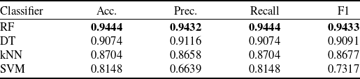
Table 8 reports the healthy-versus-any-fault task. Every classifier improves noticeably. RF reaches 94.44% accuracy with an F1 of 94.33%. DT reaches 90.74%. kNN and SVM reach 87.04% and 81.48%, respectively. The improvement from multi-class to binary is between 11 and 15 percentage points across classifiers. The information required to indicate that ‘something is wrong’ is much more readily extracted from the data than the information required to identify which specific defect is present.

Table 8.

Binary classification results (healthy vs. any fault) on the held-out 30% test set

Table 8. Long description

Table 8: For the binary healthy-versus-any-fault task the results are: Random Forest 0.9444, 0.9432, 0.9444, 0.9433. Decision Tree 0.9074, 0.9116, 0.9074, 0.9091. kNN 0.8704, 0.8658, 0.8704, 0.8677. SVM 0.8148, 0.6639, 0.8148, 0.7317 (accuracy, precision, recall, F1). Random Forest is best on all metrics, and every classifier improves substantially relative to the seven-class task.

Note: Bold values indicate the best result in each column.

Table 9.

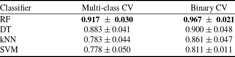
Five-fold stratified cross-validation accuracy. Mean $\pm$ standard deviation across folds

Table 9. Long description

Table 9: The table gives mean cross-validation accuracy plus or minus the standard deviation across folds, multi-class then binary. Random Forest: 0.917 plus or minus 0.030, and 0.967 plus or minus 0.021. Decision Tree: 0.883 plus or minus 0.041, and 0.900 plus or minus 0.048. kNN: 0.783 plus or minus 0.044, and 0.861 plus or minus 0.047. SVM: 0.778 plus or minus 0.050, and 0.811 plus or minus 0.011. Random Forest ranks highest on both tasks and the ranking is stable across folds.

Note: Bold values indicate the best result in each column.

4.5 Cross-validation

Held-out scores from a single split can be misleading on a small dataset. Table 9 reports the five-fold stratified cross-validation results. RF yields a mean accuracy of 91.67% on the multi-class task and 96.67% on the binary task. The standard deviations are sufficiently small that the ranking among classifiers remains stable across folds. Figure 9 visualises the same information.

Figure 9.

Five-fold stratified cross-validation results for all classifiers on both classification tasks.

Figure 9. Long description

Figure 9: A grouped bar chart of mean five-fold cross-validation accuracy with error bars showing the standard deviation across folds, for Random Forest, Decision Tree, kNN and SVM on both the seven-class and the binary tasks. Random Forest is highest on both, at 0.917 plus or minus 0.030 for the multi-class task and 0.967 plus or minus 0.021 for the binary task. Decision Tree follows at 0.883 and 0.900, then kNN at 0.783 and 0.861, and SVM lowest at 0.778 and 0.811. Binary accuracy exceeds multi-class accuracy for every classifier.

Figure 10.

Side-by-side comparison of classifier performance on the multi-class and binary tasks.

Figure 10. Long description

Figure 10: A summary bar chart placing the held-out test scores and the five-fold cross-validation scores side by side for Random Forest, Decision Tree, kNN and SVM, on both the multi-class and binary tasks. The two ensemble-tree methods, Random Forest and Decision Tree, occupy the top of the ranking in every view, with Random Forest highest overall. kNN is intermediate and SVM is consistently the weakest, reflecting the small sample size relative to the 27-dimensional feature space.

Figure 10 places the held-out and CV results side by side. The ensemble methods occupy the top of the ranking in both views. SVM is the weakest, which is attributed to the small dataset combined with the 27-dimensional feature space; RBF SVMs require careful tuning of $C$ and $\gamma$ that a 180-sample dataset cannot adequately support. kNN sits in the middle and is penalised by the high-feature dimensionality relative to sample count.

5.1 Why RF performs best here

RF behaves well on the type of data considered. The features are heterogeneous – means and higher moments lie on quite different numerical scales – the sample size is small, and the class boundary is nonlinear. Trees handle heterogeneous scales without preprocessing tricks. Bagging across 100 trees yields a usable variance reduction even with fewer than 200 windows. In addition, the Gini importance provides a free interpretability benefit that supports the qualitative analysis in Section 4. This combination of an explicit feature definition followed by a compact classical model has been adopted productively in other analytical-to-AI pipelines outside the UAV domain. A recent example is the entropy-generation analysis of pulsating non-Newtonian heat flow [Reference Altunkaya, Ozkat and Avci32], where the analytical model defines the descriptors and a learned model selects between regimes.

DT performs almost as well on the binary task but is more brittle in the multi-class setting. SVM and kNN both suffer from the dimensionality-to-sample-size ratio. None of these observations is surprising; the more interesting question concerns the magnitude of the gap between the binary and multi-class tasks.

5.2 The binary–multi-class gap

On the binary task, the classifier is effectively asked to separate a low-vibration cluster (Healthy, together with the low-amplitude Fault-2/3/5 group when quiescent) from a high-vibration cluster (Fault-1/4/6). This separation is robust, and even simple statistics such as the Y-axis standard deviation are sufficient to recover most of it. On the multi-class task, the classifier must discriminate within those clusters, and within the low-vibration cluster the univariate moments are insufficient.

The multi-class accuracy could potentially be improved by adopting a more expressive feature set: frequency-domain features (if the sampling rate permitted), envelope spectra or learned representations. However, the binding constraint is judged to be data volume rather than feature design. With only seven windows for Fault-2, the classifier has very little to learn from. A useful next experiment would be to fly several short repeat runs of the low-amplitude faults rather than a single long run for each.

5.3 Rationale for not using SMOTE

Class imbalance is non-trivial here: 34 windows for Healthy against 7 for Fault-2. The standard response is to oversample with SMOTE or a related technique. This option was not adopted, for two reasons. First, the synthetic minority oversampling technique (SMOTE) synthesises new samples by interpolating between existing minority-class neighbours in feature space, but with only seven Fault-2 windows the neighbour structure is too sparse to support meaningful interpolation without introducing artefacts. Second, the class imbalance reflects a real physical asymmetry: severe faults cut flights short, and the operational use case of the classifier already accommodates the possibility of a flight ending early. Cost-sensitive learning, or stratified collection of additional data, are cleaner remedies than synthetic oversampling.

5.4 Comparison with deep learning on similar platforms

A natural question concerns how the present approach compares with deep methods on UAV vibration data. Reviews of deep learning for machinery health monitoring report that convolutional and recurrent architectures generally need training sets one to two orders of magnitude larger than the one used here before they begin to outperform careful classical baselines [Reference Saufi, Ahmad, Leong and Lim10–Reference Khan and Yairi12]. A parallel observation is made in the recent aerospace prognostics literature: deep and similarity-based pipelines for turbofan remaining-useful-life prediction on the Commercial Modular Aero-Propulsion System Simulation (C-MAPSS) benchmark improve over classical baselines only once the training set covers a substantial portion of the degradation trajectory [Reference Isbilen, Bektas and Konar33, Reference Isbilen, Bektas, Avsar and Konar34], and the benefit is much weaker when only a handful of run-to-failure traces are available. The pattern is consistent: deep models scale well when data are plentiful and become wasteful or unstable when they are not. For a small operator able to conduct an afternoon of test sorties, the present result suggests starting with RF on hand-crafted moments and moving to a deep model only when the data budget justifies it. It should be acknowledged that no deep baseline was trained on the present dataset; the comparison above rests on the cited literature rather than on a controlled experiment on these 180 windows, and a compact one-dimensional convolutional baseline on the same protocol is planned so that the overfitting argument can be made empirically. Relatedly, because the Gini ranking (section 4.3) concentrates the discriminative weight in roughly five amplitude-dispersion features, a reduced or explicitly selected feature set is expected to particularly benefit the distance- and margin-based classifiers (kNN and SVM) that are penalised by the present 27-dimensional space; a feature-selection study is left for the extended dataset.

5.5 Towards onboard real-time deployment

The classifier itself is computationally inexpensive. A trained RF with 100 shallow trees fits readily on a Pixhawk-class or Cube Orange-class flight controller, and the 27 features can be computed on a rolling 10 s buffer in tens of milliseconds. The more demanding engineering questions lie upstream: a higher-rate accelerometer link without the present Wi-Fi packet-loss issue, a wired serial peripheral interface (SPI) or I $^{2}$ C connection from the sensor into the autopilot, and a clear policy on the autopilot response when the classifier raises a flag. A plausible candidate policy is a ‘return to launch’ instruction triggered by persistent binary fault detection across several consecutive windows, which keeps the false-alarm cost low and leaves the operator with an opportunity to override. The validity of such a policy depends on the false-positive and false-negative rates measured under conditions broader than the present indoor campaign, and must be established empirically before any deployment. In this sense the wireless pipeline demonstrated here should be read as a low-cost demonstrator that establishes the amplitude-based detectability floor, rather than as the production sensing architecture; a fielded monitor is expected to adopt the wired, higher-rate link discussed above. For a safety function the governing metric is the false-negative (missed-fault) rate rather than the overall accuracy, and this rate together with its confidence interval must be characterised under broader conditions before any return-to-launch rule is enabled. No safety claim is made on the basis of the present indoor dataset.

The transferability of the present pipeline to fixed-wing UAVs is an open question. A single-propeller fixed-wing platform reframes the multi-class problem from ‘which rotor is degraded’ to ‘which damage mode is present’ on the one propulsor. The vibration channel may also be less crowded because rotor-to-rotor harmonic interactions are not present. Whether these factors translate into improved detection or classification accuracy in practice is not something the present multirotor dataset can establish; targeted experiments on a fixed-wing platform would be required to address the question directly.

5.6 Limitations

Several limitations should be noted directly. The dataset is small, comprising 180 windows in total, of which two classes contain fewer than 15 samples each. Each propeller condition was also represented by a single flight rather than by repeated flights under the same condition, so the present dataset does not separate within-condition flight-to-flight variability from between-condition fault signature variability. Future campaigns should therefore acquire multiple independent flights per fault condition, in addition to longer individual recordings, in order to support a proper repeated-measures analysis of classifier confidence. The end-to-end sampling rate of approximately 10 Hz imposed by the Wi-Fi link precludes any frequency-domain analysis above the lower harmonics of the rotor. The test conditions are benign, consisting of indoor flights with no wind and a single pilot; outdoor operation in gusty conditions would introduce a low-frequency confounder that the present preprocessing does not address. Three further limitations follow from the single-flight design and must temper the interpretation of the reported accuracies. First, because the windows are drawn from one continuous flight per condition with 50% overlap, the random 70/30 split and the stratified cross-validation may place temporally adjacent, and therefore correlated, windows in both the training and the test partitions; the reported accuracies should accordingly be interpreted as a measure of within-flight discriminability, and a group-aware evaluation (leave-one-flight-out, with several independent flights per condition) is required before any claim of between-flight operational generalisation can be made. Second, the single motor-mount accelerometer observes primarily the rotor nearest to it, so the present results characterise detection when the degraded propeller is the instrumented one; detecting damage on a non-instrumented rotor would require additional sensors or the exploitation of cross-airframe propagation. Third, the defects are reversible mass-perturbation surrogates, which reproduce imbalance-driven excitation but not the stiffness and aeroelastic changes associated with genuine material loss such as cracks or leading-edge erosion; at least one real material-removal defect will be included in the extended campaign to anchor the surrogate against an in-service fault. The next iteration of the experimental campaign is planned to address these limitations together.