1 Introduction
The motion of a non-aqueous phase (be it a gas bubble or an oil droplet) along a capillary that is initially filled with an aqueous liquid was first analysed by Bretherton in what is now a classical fluid mechanics study (see Bretherton Reference Bretherton1961). The pressure drop needed to drive the bubble or droplet along is found to be a capillary pressure (i.e. the surface or interfacial tension divided by the capillary radius) plus a correction due to the speed at which the bubble or droplet is moving. The surprising result found by Bretherton (Reference Bretherton1961) is that this correction is nonlinear in the bubble/droplet speed. The reason for this nonlinearity is that the viscous dissipation leading to the aforementioned pressure drop correction arises from a so called transition region in which a uniformly curved capillary static interface joins up with an aqueous thin film lining the capillary wall: see figure 1. Since the length and thickness of the transition region turn out to be nonlinear functions of the bubble/droplet speed, the dissipative pressure drop across the transition region is also nonlinear (Bretherton Reference Bretherton1961; Park & Homsy Reference Park and Homsy1984).
The theory of Bretherton and various extensions thereof (e.g. Ro & Homsy Reference Ro and Homsy1995; Giavedoni & Saita Reference Giavedoni and Saita1997; Heil Reference Heil2001; Hazel & Heil Reference Hazel and Heil2002; Severino, Giavedoni & Saita Reference Severino, Giavedoni and Saita2003; Ubal et al. Reference Ubal, Campana, Giavedoni and Saita2008; Laborie et al. Reference Laborie, Rouyer, Angelescu and Lorenceau2017) have numerous applications in fields such as foam dynamics (Reinelt & Kraynik Reference Reinelt and Kraynik1990; Cantat, Kern & Delannay Reference Cantat, Kern and Delannay2004; Green et al. Reference Green, Bramley, Lue and Grassia2006; Saugey, Drenckhan & Weaire Reference Saugey, Drenckhan and Weaire2006), microfluidics (Cantat Reference Cantat2013) or gas-assisted injection of a polymeric liquid into a mould (Gauri & Koelling Reference Gauri and Koelling1999). One important application however is in oil recovery. Here one has (Cobos, Carvalho & Alvarado Reference Cobos, Carvalho and Alvarado2009) a small oil droplet located within a capillary pore in an oil reservoir. The oil droplet is typically in contact with water, and an injection fluid (itself water in the case of waterflooding (Willhite Reference Willhite1986)) is then injected into the pore to drive the oil out: a Bretherton-like problem then results.
An issue highlighted by Wilmott and co-workers in a recent study (Wilmott, Breward & Chapman Reference Wilmott, Breward and Chapman2018) is that the surfaces of the oil drop and the surrounding pore wall (typically comprised of clay) can be charged. As a result, as the droplet moves along, it is necessary to account for not just capillary forces and viscous dissipation forces, but electrostatic forces also, which (depending on the surface charges present) can be either disjoining or conjoining in nature. Models incorporating such forces have been considered by Teletzke, Davis & Scriven (Reference Teletzke, Davis and Scriven1987, Reference Teletzke, Davis and Scriven1988): it was shown that disjoining forces make the aqueous film lining the capillary wall thicker, whereas conjoining forces make it thinner. That said, the faster the droplet moves, the thicker the aqueous film it leaves behind, and (since electrostatic forces are screened with distance) the classical Bretherton (Reference Bretherton1961) theory could then be recovered.
Another complication is that the water used to displace oil might have various different levels of salinity (Yildiz & Morrow Reference Yildiz and Morrow1996; McGuire et al. Reference McGuire, Chatham, Paskvan, Sommer and Carini2005; Lager et al. Reference Lager, Webb, Black, Singleton and Sorbie2008; Ligthelm et al. Reference Ligthelm, Gronsveld, Hofman, Brussee, Marcelis and van der Linde2009; Lee et al. Reference Lee, Webb, Collins, Lager, Clarke, O’Sullivan, Routh and Wang2010; RezaeiDoust, Puntervold & Austad Reference RezaeiDoust, Puntervold and Austad2011). This presents a double complication in fact: not only does salinity affect the distance over which electrostatic forces are screened (Wright Reference Wright2007), but also the charge state of the oil and capillary wall surfaces can be sensitive to salinity. As explained by Wilmott et al. (Reference Wilmott, Breward and Chapman2018), the oil and capillary wall surfaces (the latter typically considered to be comprised of clay) tend to be negatively charged in low salinity environments, but these surfaces also contain adsorption sites. As the water salinity increases, positive ions adsorb to the surfaces, tending to reduce the magnitude of the surface charges (i.e. make the charge less negative). If the water contains a mix of monovalent and divalent positive ions, adsorption of the divalent ions can overcompensate for the original negative charges: in this case the net sign of the charge on each surface can switch from negative to positive.
Sketch of an oil droplet moving into a capillary initially filled with an aqueous phase containing ions. From left to right there is an aqueous thin film, a transition region and a capillary static region: the shapes of these regions are affected by charges on the droplet surface and on the walls of the capillary. In the frame of reference of the droplet (as is shown here) the front of the droplet is not moving, but the capillary walls (and the thin film) move to the left.

It was already recognised by Teletzke et al. (Reference Teletzke, Davis and Scriven1988), that salinity levels and surface charges would influence electrostatic forces across films, but an explicit representation of how that influence would manifest itself was left unspecified. Values of parameters governing the electrostatic behaviour in oil recovery were however estimated by Wilmott et al. (Reference Wilmott, Breward and Chapman2018) using a set of data from the literature (Lewis Reference Lewis1937; Joseph Reference Joseph1946; Malmberg & Maryott Reference Malmberg and Maryott1956; Fletcher & Sposito Reference Fletcher and Sposito1989; Buckley Reference Buckley1996; Fournier et al. Reference Fournier, Oelkers, Gout and Pokrovski1998; Li & Xu Reference Li and Xu2008; Nelson Reference Nelson2009; Austad, RezaeiDoust & Puntervold Reference Austad, RezaeiDoust and Puntervold2010), and the effects of varying salinity for that particular parameter set were considered. However one aspect that was not explored in detail is that parameters governing the surface physical chemistry, e.g. density of adsorption sites on the capillary wall/clay and the oil (obtained from Lewis (Reference Lewis1937), Li & Xu (Reference Li and Xu2008)), and also the affinity of those sites for adsorption (obtained from Fletcher & Sposito (Reference Fletcher and Sposito1989), Fournier et al. (Reference Fournier, Oelkers, Gout and Pokrovski1998), Joseph (Reference Joseph1946)), are likely to be very sensitive to the chemical composition of the system. Thus, for different compositions, it may be possible to observe a much wider class of behaviours than those predicted by Wilmott et al. (Reference Wilmott, Breward and Chapman2018). In this work we consider a wider set of surface charge states for a capillary containing an oil droplet, and determine the implications for both the thickness of the aqueous film (left behind on the capillary wall as the oil droplet advances) and the correction to the capillary pressure drop due to viscous and/or electrostatic effects.
This work is laid out as follows. In § 2 we describe the mathematical model for the system under consideration and present the overarching governing equation. Then in § 3 we present the methodology used to solve the governing equation and we also evaluate model parameters. After that, results predicted by the model are presented in § 4, and then § 5 offers discussion and conclusions.
2 Model and governing equations
This section is laid out as follows. Section 2.1 presents the overarching governing equation for oil droplet motion within a capillary pore. Next in § 2.2 the governing equation is rescaled into a more useful form. Parameters that influence the behaviour of the governing equation are discussed in §§ 2.3–2.4. The technique for evaluating the pressure drop associated with the oil droplet motion is described in § 2.5.
2.1 Governing equation
The problem under consideration has already been formulated by Wilmott et al. (Reference Wilmott, Breward and Chapman2018) so only brief summary details of the main governing equation are given here. The notation used here is slightly different from the study of Wilmott et al. (Reference Wilmott, Breward and Chapman2018). The reason is that the study in question considered that a given pressure difference was applied and determined the speed of advance of the droplet as part of the solution of the problem. A capillary number was therefore defined in terms of the known applied pressure rather than the a priori unknown droplet speed. Here however we adopt a simpler approach in which the droplet speed is treated as given. The capillary number then becomes
 $\unicode[STIX]{x1D707}V/\unicode[STIX]{x1D6FE}$
where
 $\unicode[STIX]{x1D707}$
is aqueous phase viscosity,
 $V$
is droplet speed and
 $\unicode[STIX]{x1D6FE}$
is the interfacial tension between the oil and aqueous phase. This corresponds to the definition used in the original formulation of Bretherton (Reference Bretherton1961), so we denote it
 $Ca_{B}$
(so as not to confuse it with the alternative definition of capillary number employed by Wilmott et al. (Reference Wilmott, Breward and Chapman2018)).
Solving the problem for advance of an oil droplet requires solving for the shape of the aqueous film that separates the droplet from the capillary wall: see figure 1. In the interests of simplicity we assume a two-dimensional case (rather than an axisymmetric system) with the half-thickness of the capillary being denoted
 $R$
. A static drop in the capillary would then have a curvature radius exactly equal to
 $R$
on its front and back ends. Here however the droplet is moving, so the curvature radius can be perturbed slightly. The droplet shape can in principle be affected by the ratio between the droplet viscosity and aqueous phase viscosity. However analysis by Park & Homsy (Reference Park and Homsy1984) has suggested that, provided the viscosity ratio is no larger than order
 $Ca_{B}^{-1/3}$
(with
 $Ca_{B}\ll 1$
in problems of interest), then the viscosity ratio has no bearing on the shape.
As alluded to earlier, uniformly curved capillary static regions at the ends of the drop are joined up with an aqueous thin film across a transition region. Determining the shape of the transition region then becomes part of the required solution. In what follows, unless explicitly specified otherwise, we will employ the term ‘thin film’ to refer to the thinnest part excluding the transition region, and the term ‘film’ more generically including possibly the transition region in addition to the thinnest part. It turns out moreover that the shape of the transition region near the rear of the drop (Burgess & Foster Reference Burgess and Foster1990; Wong, Radke & Morris Reference Wong, Radke and Morris1995a ,Reference Wong, Radke and Morris b ; Giavedoni & Saita Reference Giavedoni and Saita1999; Wilmott et al. Reference Wilmott, Breward and Chapman2018) is a little more complex than the shape near the front. In the interests of simplicity therefore we focus here solely on the region at the front of the drop.
We switch to a frame of reference moving with the drop. In this frame of reference, the shape of the drop (i.e. the thickness of the transition region versus distance along it) should have attained a steady state. Hence an ordinary differential equation (rather than a partial differential equation) can be solved. In what follows, equations are cast in dimensionless form. Both thickness and distance are scaled by
 $R$
, pressures are scaled by
 $\unicode[STIX]{x1D6FE}/R$
and velocities are scaled by
 $\unicode[STIX]{x1D6FE}/\unicode[STIX]{x1D707}$
. The governing equation for dimensionless aqueous film thickness
 $h$
versus dimensionless distance
 $Z$
along the film (which is derived in appendix A following Wilmott et al. (Reference Wilmott, Breward and Chapman2018)) is then
 $$\begin{eqnarray}h_{ZZZ}=3Ca_{B}\frac{(h-h^{\ast })}{h^{3}}-\frac{1}{\bar{\unicode[STIX]{x1D6E4}}}\left(\frac{\unicode[STIX]{x1D70E}_{c0}^{2}+2s^{\ast }\unicode[STIX]{x1D70E}_{c0}\unicode[STIX]{x1D70E}_{o0}\cosh (h/\unicode[STIX]{x1D716}_{2})+s^{\ast \,2}\unicode[STIX]{x1D70E}_{o0}^{2}}{\sinh ^{2}(h/\unicode[STIX]{x1D716}_{2})}\right)_{Z},\end{eqnarray}$$
where
 $Ca_{B}$
is the capillary number,
 $h^{\ast }$
is the uniform film thickness outside the transition region (which is a priori unknown),
 $\bar{\unicode[STIX]{x1D6E4}}$
is a parameter (precise mathematical definition to be given shortly) measuring the relative importance of capillary and electrostatic terms (specifically referred to electrostatics on the capillary wall) and
 $\unicode[STIX]{x1D716}_{2}$
(again precise mathematical definition to be given shortly) is the ratio between a Debye screening length (Wright Reference Wright2007) and channel half-thickness
 $R$
.
The bracketed term on the right-hand side of (2.1) represents an electro-osmotic tension (Yang, Fu & Hwang Reference Yang, Fu and Hwang2001; Waghmare & Mitra Reference Waghmare and Mitra2008). The parameter
 $\unicode[STIX]{x1D70E}_{c0}$
is the net charge per adsorption site on the capillary wall,
 $\unicode[STIX]{x1D70E}_{o0}$
is the charge per adsorption site on the oil and
 $s^{\ast }$
is the ratio between the density of adsorption sites on the oil and on the wall. Note that both
 $\unicode[STIX]{x1D70E}_{c0}$
and
 $\unicode[STIX]{x1D70E}_{o0}$
can vary in principle between
 $-1$
(corresponding to all of the negatively charged adsorption sites remaining unoccupied) and
 $+1$
(corresponding to all adsorption sites being occupied by divalent positive ions). Moreover
 $h/\unicode[STIX]{x1D716}_{2}$
is the ratio between film thickness and Debye screening length. In general it is necessary to consider the full
 $h/\unicode[STIX]{x1D716}_{2}$
dependence of the electro-osmotic tension in (2.1), which is relatively complicated. There are however some simpler limiting cases considered in appendix B. In particular, if
 $h/\unicode[STIX]{x1D716}_{2}\gg 1$
electrostatic effects are screened by electrical double layer effects, and so are weak regardless of the value of
 $\bar{\unicode[STIX]{x1D6E4}}$
. The electro-osmotic tension then reduces to an exponential decay, a case considered by Teletzke et al. (Reference Teletzke, Davis and Scriven1988).
2.2 Rescaling the governing equation
In order to solve the governing equation (2.1), a number of manipulations are required. These are standard in the Bretherton case (ignoring electrostatic effects), but in what follows we review how they are modified in the presence of electrostatic terms. It is known that (Bretherton Reference Bretherton1961) the length and thickness of the transition region scale respectively as
 $Ca_{B}^{1/3}$
and
 $Ca_{B}^{2/3}$
, scalings that apply at least nominally in the Bretherton case for which electrostatic effects are neglected. It is then convenient to define new variables
 $\unicode[STIX]{x1D6F9}=Z/(3Ca_{B})^{1/3}$
and
 $J=h/(3Ca_{B})^{2/3}$
. Equation (2.1) then becomes
 $$\begin{eqnarray}J_{\unicode[STIX]{x1D6F9}\unicode[STIX]{x1D6F9}\unicode[STIX]{x1D6F9}}=\frac{(J-J^{\ast })}{J^{3}}-\frac{1}{\bar{\unicode[STIX]{x1D6E4}}}\left(\frac{\unicode[STIX]{x1D70E}_{c0}^{2}+2s^{\ast }\unicode[STIX]{x1D70E}_{c0}\unicode[STIX]{x1D70E}_{o0}\cosh (J\,\unicode[STIX]{x1D712}^{\prime })+s^{\ast \,2}\unicode[STIX]{x1D70E}_{o0}^{2}}{\sinh ^{2}(J\,\unicode[STIX]{x1D712}^{\prime })}\right)_{\unicode[STIX]{x1D6F9}},\end{eqnarray}$$
where
 $J^{\ast }$
is the value of
 $J$
in the thin film region, and
 $\unicode[STIX]{x1D712}^{\prime }\equiv (3Ca_{B})^{2/3}/\unicode[STIX]{x1D716}_{2}$
(the ratio between the characteristic or ‘nominal’ film thickness according to Bretherton (Reference Bretherton1961) and the Debye screening length (Wright Reference Wright2007)).
Since the capillary number has been scaled out, we expect
 $J^{\ast }$
just to be a function of the remaining parameters
 $\bar{\unicode[STIX]{x1D6E4}}$
,
 $\unicode[STIX]{x1D70E}_{c0}$
,
 $\unicode[STIX]{x1D70E}_{o0}$
,
 $s^{\ast }$
and
 $\unicode[STIX]{x1D712}^{\prime }$
. The issue however is that
 $J^{\ast }$
is a priori unknown and must be solved as part of the solution of the problem. This is addressed by rescaling yet again, introducing variables
 $G=J/J^{\ast }$
and
 $\unicode[STIX]{x1D701}=\unicode[STIX]{x1D6F9}/J^{\ast }$
. We also define
 $$\begin{eqnarray}\displaystyle & \displaystyle \unicode[STIX]{x1D6E4}^{\ast }(\bar{\unicode[STIX]{x1D6E4}},J^{\ast })=\bar{\unicode[STIX]{x1D6E4}}/J^{\ast } & \displaystyle\end{eqnarray}$$
 $$\begin{eqnarray}\displaystyle & \displaystyle \unicode[STIX]{x1D712}^{\ast }(\unicode[STIX]{x1D712}^{\prime },J^{\ast })=\unicode[STIX]{x1D712}^{\prime }J^{\ast }. & \displaystyle\end{eqnarray}$$
The resulting equation is
 $$\begin{eqnarray}G_{\unicode[STIX]{x1D701}\unicode[STIX]{x1D701}\unicode[STIX]{x1D701}}=\frac{(G-1)}{G^{3}}-\frac{1}{\unicode[STIX]{x1D6E4}^{\ast }}\left(\frac{\unicode[STIX]{x1D70E}_{c0}^{2}+2s^{\ast }\unicode[STIX]{x1D70E}_{c0}\unicode[STIX]{x1D70E}_{o0}\cosh (G\,\unicode[STIX]{x1D712}^{\ast })+s^{\ast \,2}\unicode[STIX]{x1D70E}_{o0}^{2}}{\sinh ^{2}(G\,\unicode[STIX]{x1D712}^{\ast })}\right)_{\unicode[STIX]{x1D701}}\end{eqnarray}$$
the final term in brackets as in (2.1) representing the electro-osmotic tension.
We now know that in the thin film region (for small
 $\unicode[STIX]{x1D701}$
)
 $G\rightarrow 1$
, whereas as we approach the capillary static region (for large
 $\unicode[STIX]{x1D701}$
)
 $G_{\unicode[STIX]{x1D701}\unicode[STIX]{x1D701}}$
must approach some asymptotic value (this follows because the right-hand side of (2.5) vanishes for large
 $G$
). We denote this large
 $\unicode[STIX]{x1D701}$
asymptotic value by
 $G_{\unicode[STIX]{x1D701}\unicode[STIX]{x1D701},\infty }$
. Based on the way in which we have defined
 $G$
,
 $\unicode[STIX]{x1D701}$
,
 $J$
and
 $\unicode[STIX]{x1D6F9}$
in terms of
 $h$
and
 $Z$
it follows that
 $G_{\unicode[STIX]{x1D701}\unicode[STIX]{x1D701}}=J^{\ast }J_{\unicode[STIX]{x1D6F9}\unicode[STIX]{x1D6F9}}=J^{\ast }h_{ZZ}$
. Since
 $h_{ZZ}$
is expected to approach unity in the capillary static region, knowing
 $G_{\unicode[STIX]{x1D701}\unicode[STIX]{x1D701},\infty }$
is sufficient to give
 $J^{\ast }$
. Equation (2.5) can therefore be solved numerically (for any given
 $\unicode[STIX]{x1D6E4}^{\ast }$
,
 $\unicode[STIX]{x1D712}^{\ast }$
,
 $\unicode[STIX]{x1D70E}_{c0}$
,
 $\unicode[STIX]{x1D70E}_{o0}$
and
 $s^{\ast }$
) and hence the corresponding value of
 $G_{\unicode[STIX]{x1D701}\unicode[STIX]{x1D701},\infty }$
can be determined.
In the Bretherton case, finding
 $G_{\unicode[STIX]{x1D701}\unicode[STIX]{x1D701},\infty }$
completes the solution of the problem. In the presence of electro-osmotic terms, however this is not the full solution to the problem, because
 $G_{\unicode[STIX]{x1D701}\unicode[STIX]{x1D701},\infty }$
has been computed for values
 $\unicode[STIX]{x1D6E4}^{\ast }$
and
 $\unicode[STIX]{x1D712}^{\ast }$
but these are not given a priori, but rather are themselves functions of
 $J^{\ast }$
according to (2.3)–(2.4). We are therefore required to vary a guessed value for
 $J^{\ast }$
(for fixed
 $\bar{\unicode[STIX]{x1D6E4}}$
and
 $\unicode[STIX]{x1D712}^{\prime }$
and therefore variable
 $\unicode[STIX]{x1D6E4}^{\ast }$
and
 $\unicode[STIX]{x1D712}^{\ast }$
) and keep computing
 $G_{\unicode[STIX]{x1D701}\unicode[STIX]{x1D701},\infty }$
until the computed
 $G_{\unicode[STIX]{x1D701}\unicode[STIX]{x1D701},\infty }$
equals the guessed
 $J^{\ast }$
.
Finding the required
 $J^{\ast }$
that satisfies that condition is straightforward if we first solve the Bretherton problem with no electro-osmotic effects to obtain a well-defined value
 $J_{B}^{\ast }$
, and then recall that a disjoining electro-osmotic tension leads to thicker films (and so must have
 $J^{\ast }>J_{B}^{\ast }$
) whereas a conjoining electro-osmotic pressure leads to thinner films (and so has
 $J^{\ast }<J_{B}^{\ast }$
). Moreover cases with large
 $\bar{\unicode[STIX]{x1D6E4}}$
and/or large
 $\unicode[STIX]{x1D712}^{\prime }$
have weak electro-osmotic effects and hence must be close to the Bretherton case, meaning that we can easily work downwards from large
 $\bar{\unicode[STIX]{x1D6E4}}$
and/or
 $\unicode[STIX]{x1D712}^{\prime }$
to smaller values of these parameters.
2.3 Parameters
 $\bar{\unicode[STIX]{x1D6E4}}$
and
$\unicode[STIX]{x1D716}_{2}$


Earlier we gave the physical interpretation of
 $\bar{\unicode[STIX]{x1D6E4}}$
and
 $\unicode[STIX]{x1D716}_{2}$
but did not give actual formulae.
Specifically
 $\bar{\unicode[STIX]{x1D6E4}}$
is defined as
 $$\begin{eqnarray}\bar{\unicode[STIX]{x1D6E4}}=2\unicode[STIX]{x1D6FE}\unicode[STIX]{x1D700}_{w}/Rq^{2}s_{c}^{\ast \,2},\end{eqnarray}$$
where
 $\unicode[STIX]{x1D6FE}$
is interfacial tension,
 $\unicode[STIX]{x1D700}_{w}$
is electrical permittivity of the aqueous phase,
 $R$
is half-thickness of the capillary,
 $q$
is the electronic charge,
 $s_{c}^{\ast }$
is the density of adsorption sites on the wall. Note that Wilmott et al. (Reference Wilmott, Breward and Chapman2018) employed a related parameter
 $\unicode[STIX]{x1D6E4}$
in lieu of
 $\bar{\unicode[STIX]{x1D6E4}}$
with a slightly different definition, but in the formulation that we present
 $\bar{\unicode[STIX]{x1D6E4}}$
is the more convenient parameter. Observe (see e.g. (2.1) or (2.5)) that the larger the value of
 $\bar{\unicode[STIX]{x1D6E4}}$
the less important the electro-osmotic terms. In the context of waterflooding, an increased
 $\bar{\unicode[STIX]{x1D6E4}}$
could be achieved by decreasing
 $R$
(although it would be challenging to extract oil from a rock with extremely narrow pores) or by reducing the surface density of adsorption sites (which presumably could be achieved by changing the chemistry of the clay comprising the capillary wall).
The parameter
 $\unicode[STIX]{x1D716}_{2}$
is the electrical double layer thickness non-dimensionalised by
 $R$
 $$\begin{eqnarray}\unicode[STIX]{x1D716}_{2}=(\unicode[STIX]{x1D700}_{w}k_{B}T/(2(C^{+}+4C^{2+})q^{2}R^{2}))^{1/2},\end{eqnarray}$$
where
 $\unicode[STIX]{x1D700}_{w}$
is the electric permittivity of the aqueous phase,
 $k_{B}$
is Boltzmann’s constant,
 $T$
is absolute temperature,
 $q$
is electronic charge,
 $C^{+}$
is number density of monovalent ions and
 $C^{2+}$
is number density of divalent ions. However, the parameter that determines whether or not electro-osmotic effects are screened across the aqueous layer is
 $\unicode[STIX]{x1D712}^{\prime }$
(itself introduced in (2.2)) which evaluates to
 $$\begin{eqnarray}\unicode[STIX]{x1D712}^{\prime }\equiv (3Ca_{B})^{2/3}/\unicode[STIX]{x1D716}_{2}=(3Ca_{B})^{2/3}(2(C^{+}+4C^{2+})q^{2}R^{2}/\unicode[STIX]{x1D700}_{w}k_{B}T)^{1/2}.\end{eqnarray}$$
Note that Wilmott et al. (Reference Wilmott, Breward and Chapman2018) employed a related parameter
 $\unicode[STIX]{x1D712}$
in lieu of
 $\unicode[STIX]{x1D712}^{\prime }$
with a slightly different definition: in the formulation presented here, using the parameter
 $\unicode[STIX]{x1D712}^{\prime }$
turns out to be more convenient. Larger
 $\unicode[STIX]{x1D712}^{\prime }$
implies more effective charge screening making electro-osmotic terms less relevant. Practical ways of altering
 $\unicode[STIX]{x1D712}^{\prime }$
when recovering oil from a given formation include injecting fluid at a different speed (in effect changing the capillary number) or varying the salinity (changing
 $C^{+}$
and/or
 $C^{2+}$
). In typical systems of interest, the number density of monovalent ions
 $C^{+}$
tends to be rather larger than that of divalent ions
 $C^{2+}$
meaning that to a good approximation
 $\unicode[STIX]{x1D712}^{\prime }\propto (C^{+})^{1/2}$
. As will be discussed below, changing
 $C^{+}$
and/or
 $C^{2+}$
not only affects
 $\unicode[STIX]{x1D712}^{\prime }$
but also has a side effect of changing the charge states of the wall and oil surfaces, denoted
 $\unicode[STIX]{x1D70E}_{c0}$
and
 $\unicode[STIX]{x1D70E}_{o0}$
. Since the electro-osmotic term in (2.2) is sensitive to all these parameters (
 $\unicode[STIX]{x1D712}^{\prime }$
,
 $\unicode[STIX]{x1D70E}_{c0}$
and
 $\unicode[STIX]{x1D70E}_{o0}$
), the net effect of changing salinity can potentially be quite complex.
2.4 Determining surface charges on the wall and oil
$\unicode[STIX]{x1D70E}_{c0}$
and
$\unicode[STIX]{x1D70E}_{o0}$


So far we have stated that the charge per adsorption site on the capillary wall
 $\unicode[STIX]{x1D70E}_{c0}$
and the oil
 $\unicode[STIX]{x1D70E}_{o0}$
can vary from
 $-1$
(no positive ions adsorbed whatsoever) to
 $+1$
(divalent positive ions adsorbed on all sites). In a number of our calculations we will, for simplicity, impose fixed values for
 $\unicode[STIX]{x1D70E}_{c0}$
and/or
 $\unicode[STIX]{x1D70E}_{o0}$
between these extremal values
 $\pm 1$
. Nevertheless we wish to establish how
 $\unicode[STIX]{x1D70E}_{c0}$
and/or
 $\unicode[STIX]{x1D70E}_{o0}$
might be determined more generally.
Following Wilmott et al. (Reference Wilmott, Breward and Chapman2018) we assume that ion adsorption is governed by a Langmuir isotherm. We suppose as above that
 $C^{+}$
and
 $C^{2+}$
are monovalent and divalent ion number densities. Moreover we suppose that there are Langmuir constants:
 $K_{c}^{1}$
(governing monovalent adsorption on the capillary wall),
 $K_{c}^{2}$
(governing divalent adsorption on the wall),
 $K_{o}^{1}$
(governing monovalent adsorption on oil) and
 $K_{o}^{2}$
(governing divalent adsorption on oil). We next define dimensionless ion concentrations
 $c^{+}$
and
 $c^{2+}$
by multiplying each ion number density through by
 $K_{c}^{1}$
, and dimensionless Langmuir constants (
 ${\mathcal{K}}_{c}^{1}$
,
 ${\mathcal{K}}_{c}^{2}$
,
 ${\mathcal{K}}_{o}^{1}$
and
 ${\mathcal{K}}_{o}^{2}$
) by dividing each Langmuir constant through by
 $K_{c}^{1}$
: by definition
 ${\mathcal{K}}_{c}^{1}$
equals unity. Note that this differs from the non-dimensionalisation procedure of Wilmott et al. (Reference Wilmott, Breward and Chapman2018) who instead made concentration dimensionless based on an arbitrary concentration that they selected, considered to be typical of a low salinity waterflood.
Dimensionless ion concentrations
 $c^{+}$
and
 $c^{2+}$
are of course affected by the electrostatic potential, with concentrations being lower in regions of positive potential, and higher in regions of negative potential. The concentrations of negatively charged balancing counter ions are affected in the opposite way. Throughout this study, as is standard in Debye–Hückel theory (Wright Reference Wright2007), we will assume that the perturbations in ion concentration induced by electrostatic effects are small compared to the unperturbed concentrations
 $c_{0}^{+}$
and
 $c_{0}^{2+}$
in the absence of electrostatics. Under this assumption then, these unperturbed concentrations
 $c_{0}^{+}$
and
 $c_{0}^{2+}$
will determine the amount of adsorption on the wall and oil surfaces, despite those surfaces having a non-zero electrostatic potential.
In the notation of Wilmott et al. (Reference Wilmott, Breward and Chapman2018), the fraction of adsorption sites on the wall occupied by adsorbed monovalent and divalent positive ions are respectively denoted
 $s_{c0}$
and
 $s_{c0}^{+}$
, the analogous fractions for adsorption on oil being
 $s_{o0}$
and
 $s_{o0}^{+}$
. In terms of the dimensionless concentrations and dimensionless Langmuir parameters these evaluate to
 $$\begin{eqnarray}\displaystyle & \displaystyle s_{c0}={\mathcal{K}}_{c}^{1}c_{0}^{+}/(1+{\mathcal{K}}_{c}^{1}c_{0}^{+}+{\mathcal{K}}_{c}^{2}c_{0}^{2+}) & \displaystyle\end{eqnarray}$$
 $$\begin{eqnarray}\displaystyle & \displaystyle s_{c0}^{+}={\mathcal{K}}_{c}^{2}c_{0}^{2+}/(1+{\mathcal{K}}_{c}^{1}c_{0}^{+}+{\mathcal{K}}_{c}^{2}c_{0}^{2+}) & \displaystyle\end{eqnarray}$$
 $$\begin{eqnarray}\displaystyle & \displaystyle s_{o0}={\mathcal{K}}_{o}^{1}c_{0}^{+}/(1+{\mathcal{K}}_{o}^{1}c_{0}^{+}+{\mathcal{K}}_{o}^{2}c_{0}^{2+}) & \displaystyle\end{eqnarray}$$
 $$\begin{eqnarray}\displaystyle & \displaystyle s_{o0}^{+}={\mathcal{K}}_{o}^{2}c_{0}^{2+}/(1+{\mathcal{K}}_{o}^{1}c_{0}^{+}+{\mathcal{K}}_{o}^{2}c_{0}^{2+}). & \displaystyle\end{eqnarray}$$
Finally the charges per adsorption site are
 $\unicode[STIX]{x1D70E}_{c0}=2s_{c0}^{+}+s_{c0}-1$
for the wall and
 $\unicode[STIX]{x1D70E}_{o0}=2s_{o0}^{+}+s_{c0}-1$
for the oil and hence
 $$\begin{eqnarray}\displaystyle & \displaystyle \unicode[STIX]{x1D70E}_{c0}=({\mathcal{K}}_{c}^{2}c_{0}^{2+}-1)/(1+{\mathcal{K}}_{c}^{1}c_{0}^{+}+{\mathcal{K}}_{c}^{2}c_{0}^{2+}) & \displaystyle\end{eqnarray}$$
 $$\begin{eqnarray}\displaystyle & \displaystyle \unicode[STIX]{x1D70E}_{o0}=({\mathcal{K}}_{o}^{2}c_{0}^{2+}-1)/(1+{\mathcal{K}}_{o}^{1}c_{0}^{+}+{\mathcal{K}}_{o}^{2}c_{0}^{2+}). & \displaystyle\end{eqnarray}$$
The subscripts ‘0’ on all these parameters (
 $s_{c0}$
,
 $s_{c0}^{+}$
,
 $s_{o0}$
,
 $s_{o0}^{+}$
,
 $\unicode[STIX]{x1D70E}_{c0}$
and
 $\unicode[STIX]{x1D70E}_{o0}$
) reflect the fact that they can be evaluated at ‘unperturbed’ concentrations
 $c_{0}^{+}$
and
 $c_{0}^{2+}$
instead of
 $c^{+}$
and
 $c^{2+}$
. Moreover in the interests of simplicity, it is assumed that sufficient ions are present in the aqueous film overall such that adsorption onto the capillary wall or oil surfaces does not lead to any significant change in ion concentration in the bulk.
To summarise, for a number of calculations we will perform, fixed values of
 $\unicode[STIX]{x1D70E}_{c0}$
and
 $\unicode[STIX]{x1D70E}_{o0}$
will be imposed. In cases however when fixed values are not imposed, equations (2.13)–(2.14) will be used instead.
2.5 Pressure drop across the droplet front
So far our discussion has focussed on finding how electro-osmotic effects affect the thin film region, specifically finding the parameter
 $J^{\ast }$
which determines the thickness of that region. Also of interest however is the pressure drop. At leading order the (dimensionless) pressure drop across the capillary static droplet front is unity, since the (dimensionless) curvature radius at the front is likewise unity. It is of interest however to determine how much the pressure drop at the front is perturbed by droplet motion. The technique for doing this was discussed by Wilmott et al. (Reference Wilmott, Breward and Chapman2018). The finding was that the dimensionless pressure drop
 $\unicode[STIX]{x0394}p$
could be expressed in the form
 $1+(3Ca_{B})^{2/3}\unicode[STIX]{x0394}p^{\ast }$
where
 $\unicode[STIX]{x0394}p^{\ast }$
could be obtained via
 $\unicode[STIX]{x0394}p^{\ast }\equiv \lim _{\unicode[STIX]{x1D701}\rightarrow \infty }(G_{\unicode[STIX]{x1D701}\unicode[STIX]{x1D701}}G-G_{\unicode[STIX]{x1D701}}^{2}/2)$
. It follows that not only must
 $G_{\unicode[STIX]{x1D701}\unicode[STIX]{x1D701}}$
have a well-defined limiting value as
 $\unicode[STIX]{x1D701}\rightarrow \infty$
at the end of the transition region (thereby determining
 $J^{\ast }$
) but also
 $G_{\unicode[STIX]{x1D701}\unicode[STIX]{x1D701}}G-G_{\unicode[STIX]{x1D701}}^{2}/2$
must have a well defined limiting value that determines
 $\unicode[STIX]{x0394}p^{\ast }$
.
This completes our presentation of the model and governing equations. To summarise the key equation we must solve is (2.5) for
 $G$
versus
 $\unicode[STIX]{x1D701}$
. The large
 $\unicode[STIX]{x1D701}$
limiting behaviour of this function
 $G$
furnishes the information we require, specifically the values of thin film thickness
 $J^{\ast }$
and the pressure drop change
 $\unicode[STIX]{x0394}p^{\ast }$
. Parameter values
 $\unicode[STIX]{x1D6E4}^{\ast }$
,
 $\unicode[STIX]{x1D712}^{\ast }$
,
 $s^{\ast }$
,
 $\unicode[STIX]{x1D70E}_{c0}$
and
 $\unicode[STIX]{x1D70E}_{o0}$
must be supplied (the first two parameters mentioned being related to
 $\bar{\unicode[STIX]{x1D6E4}}$
and
 $\unicode[STIX]{x1D712}^{\prime }$
via (2.3)–(2.4), and the final two being related, if required, to Langmuir parameters (
 ${\mathcal{K}}_{c}^{1}$
,
 ${\mathcal{K}}_{c}^{2}$
,
 ${\mathcal{K}}_{o}^{1}$
,
 ${\mathcal{K}}_{o}^{2}$
) via (2.13)–(2.14)): an interpretation of each of these parameters has been summarised in table 1. In the next section the numerical methodology for solving the equations and the choices of parameter values are detailed.
Dimensionless parameters affecting the electro-osmotic term in the model. Note that, although mentioned in the table,
 ${\mathcal{K}}_{c}^{1}\equiv 1$
by definition here.

3 Methodology and parameter values
This section is laid out as follows. In § 3.1 the numerical solution methodology is outlined, whereas §§ 3.2–3.3 deal with selection of suitable parameter values.
3.1 Numerical methodology
We have solved (2.5) using a fourth-order Runge–Kutta method (Press et al. Reference Press, Teukolsky, Vetterling and Flannery1992).
For sufficiently small
 $\unicode[STIX]{x1D701}$
we know that
 $G$
should approach unity. Meanwhile for sufficiently large
 $\unicode[STIX]{x1D701}$
we know that
 $G_{\unicode[STIX]{x1D701}\unicode[STIX]{x1D701}}$
should approach a constant. In order to be able to solve the equation, we need however, in the small
 $\unicode[STIX]{x1D701}$
limit, an initial condition for both
 $G_{\unicode[STIX]{x1D701}}$
and
 $G_{\unicode[STIX]{x1D701}\unicode[STIX]{x1D701}}$
, in addition to that for
 $G$
. Such conditions are obtained by linearising equation (2.5) setting
 $g\approx G-1$
. It follows
 $$\begin{eqnarray}g_{\unicode[STIX]{x1D701}\unicode[STIX]{x1D701}\unicode[STIX]{x1D701}}=g-g_{\unicode[STIX]{x1D701}}(\unicode[STIX]{x1D6E4}^{\ast })^{-1}\unicode[STIX]{x2202}T_{EO}/\unicode[STIX]{x2202}G|_{G=1},\end{eqnarray}$$
where
 $T_{EO}$
is the electro-osmotic tension (i.e. the expression within the brackets in the final term of (2.5)). The solution of (3.1) is
 $g=\unicode[STIX]{x1D700}\exp (\unicode[STIX]{x1D6EC}\unicode[STIX]{x1D701})$
where
 $\unicode[STIX]{x1D700}$
is an arbitrarily chosen small parameter (we set
 $\unicode[STIX]{x1D700}=10^{-5}$
) and
 $$\begin{eqnarray}\unicode[STIX]{x1D6EC}^{3}=1-\unicode[STIX]{x1D6EC}(\unicode[STIX]{x1D6E4}^{\ast })^{-1}\unicode[STIX]{x2202}T_{EO}/\unicode[STIX]{x2202}G|_{G=1}.\end{eqnarray}$$
Solving this cubic equation to determine
 $\unicode[STIX]{x1D6EC}$
is simple. It turns out that there is just one positive real root, and (at the front end of the drop, which is the case we consider here) this is the root we require (Wilmott et al.
Reference Wilmott, Breward and Chapman2018). If
 $\unicode[STIX]{x1D6E4}^{\ast }$
is large, the value of
 $\unicode[STIX]{x1D6EC}$
is close to unity, whereas if
 $\unicode[STIX]{x1D6E4}^{\ast }$
is small, the two terms on the right-hand side come into balance (if
 $\unicode[STIX]{x2202}T_{EO}/\unicode[STIX]{x2202}G|_{G=1}>0$
) or else the left-hand side comes into balance with the second term on the right (if
 $\unicode[STIX]{x2202}T_{EO}/\unicode[STIX]{x2202}G|_{G=1}<0$
). Given an initial estimate for
 $\unicode[STIX]{x1D6EC}$
we can determine the exact value by Newton–Raphson iteration. At
 $\unicode[STIX]{x1D701}=0$
we now have
 $G=1+\unicode[STIX]{x1D700}$
,
 $G_{\unicode[STIX]{x1D701}}=\unicode[STIX]{x1D700}\,\unicode[STIX]{x1D6EC}$
and
 $G_{\unicode[STIX]{x1D701}\unicode[STIX]{x1D701}}=\unicode[STIX]{x1D700}\,\unicode[STIX]{x1D6EC}^{2}$
. We integrated forward via Runge–Kutta with a step size
 $\unicode[STIX]{x1D6FF}\unicode[STIX]{x1D701}=0.1$
. The choice of step size
 $\unicode[STIX]{x1D6FF}\unicode[STIX]{x1D701}$
was dictated by the requirement that changes
 $G$
,
 $G_{\unicode[STIX]{x1D701}}$
and
 $G_{\unicode[STIX]{x1D701}\unicode[STIX]{x1D701}}$
during any given step should be small compared to the values of
 $G$
,
 $G_{\unicode[STIX]{x1D701}}$
and
 $G_{\unicode[STIX]{x1D701}\unicode[STIX]{x1D701}}$
at the start of the step. The integration proceeded until
 $G_{\unicode[STIX]{x1D701}\unicode[STIX]{x1D701}}$
had converged to 6 figures.
An issue however is that the other parameter we seek namely
 $G_{\unicode[STIX]{x1D701}\unicode[STIX]{x1D701}}G-G_{\unicode[STIX]{x1D701}}^{2}/2$
converges much more slowly than
 $G_{\unicode[STIX]{x1D701}\unicode[STIX]{x1D701}}$
does. In an attempt to obtain convergence for this parameter we allowed
 $\unicode[STIX]{x1D701}$
up to very large values (as large as 1000). In that case however both
 $G_{\unicode[STIX]{x1D701}\unicode[STIX]{x1D701}}G$
and
 $G_{\unicode[STIX]{x1D701}}^{2}/2$
are then large numbers (of the order of
 $\unicode[STIX]{x1D701}^{2}$
and hence of the order of a million) and the value we seek is the difference between these two large numbers. To overcome this, we devised techniques to accelerate the convergence, as discussed in appendix C.
3.2 Selecting parameter values:
$\unicode[STIX]{x1D712}^{\prime }$
,
$\bar{\unicode[STIX]{x1D6E4}}$
and
$s^{\ast }$


With the numerical solution technique now specified, it remains to select the sets of parameter values for which solutions will be obtained. Based on the literature, Wilmott et al. (Reference Wilmott, Breward and Chapman2018) proposed a number of parameter values for displacement of an oil droplet from a capillary. Our intention here is to consider parameter values comparable with those of Wilmott et al. (Reference Wilmott, Breward and Chapman2018), but recognising that a number of parameters are sensitive to surface physical chemistry, and these might exhibit quite wide variation depending on the chemical composition of the system (see e.g. Newcombe & Ralston (Reference Newcombe and Ralston1992) for a situation in which surface properties are strongly modified by chemistry).
We estimate a capillary number
 $Ca_{B}$
of the order of
 $10^{-7}$
. Obtaining this value requires a conversion between the definition of
 $Ca$
used by Wilmott et al. (Reference Wilmott, Breward and Chapman2018) (based on an imposed pressure) and the capillary number
 $Ca_{B}$
used here (based on an imposed injection speed). Since
 $Ca_{B}$
is proportional to injection speed we estimate that in an oil recovery operation it could vary by an order of magnitude either side of
 $10^{-7}$
depending on how the operation is realised. Meanwhile, values of the parameter
 $\unicode[STIX]{x1D716}_{2}$
(the ratio between Debye length and channel half-thickness) cited by Wilmott et al. (Reference Wilmott, Breward and Chapman2018) are between
 $1.5\times 10^{-3}$
in what they call a low salinity case (corresponding to
 $17~\text{mol}~\text{m}^{-3}$
of monovalent positive ions) and
 $2\times 10^{-4}$
(corresponding to
 $1700~\text{mol}~\text{m}^{-3}$
of monovalent positive ions).
Remembering that
 $\unicode[STIX]{x1D712}^{\prime }\equiv (3Ca_{B})^{2/3}/\unicode[STIX]{x1D716}_{2}$
, we estimate
 $\unicode[STIX]{x1D712}^{\prime }\approx 0.03$
in the low salinity case and
 $\unicode[STIX]{x1D712}^{\prime }\approx 0.22$
in the high salinity case. Given however we commented that
 $Ca_{B}$
could increase by up to an order of magnitude, and given also that
 $\unicode[STIX]{x1D712}^{\prime }$
is sensitive to the half-thickness of the pore (see (2.8)) which varies from rock to rock, it is reasonable to suppose that the domain of
 $\unicode[STIX]{x1D712}^{\prime }$
of interest is somewhere from order unity down to a couple of orders of magnitude smaller than that. To cover this domain specifically we will consider values
 $\unicode[STIX]{x1D712}^{\prime }$
equal to 5, 2, 1, 0.5, 0.2, 0.1, 0.05 and 0.02. For the
 $\unicode[STIX]{x1D712}^{\prime }$
values at the upper end of the domain charges are screened and electrostatic effects represent only a small perturbation to the original Bretherton system (Bretherton Reference Bretherton1961). For
 $\unicode[STIX]{x1D712}^{\prime }$
values at the lower end of the domain however, electrostatic effects should become very significant.
Concerning the parameter
 $\bar{\unicode[STIX]{x1D6E4}}$
, the estimate is
 $\bar{\unicode[STIX]{x1D6E4}}\approx 8$
. Obtaining this again requires a conversion from a parameter
 $\unicode[STIX]{x1D6E4}$
(used by Wilmott et al. (Reference Wilmott, Breward and Chapman2018), defined in terms of a channel length) to the parameter
 $\bar{\unicode[STIX]{x1D6E4}}$
used here (defined using a channel half-thickness). Since
 $\bar{\unicode[STIX]{x1D6E4}}$
relies on surface physical chemical properties (in particular it depends on the density of adsorption sites on the capillary wall
 $s_{c}^{\ast }$
, reported by Li & Xu (Reference Li and Xu2008)) there is likely to be considerable variation in
 $\bar{\unicode[STIX]{x1D6E4}}$
depending on chemical composition. In view of this, in the interest of simplicity, we set
 $\bar{\unicode[STIX]{x1D6E4}}=10$
(instead of the original estimated value 8). We also considered a case with an order of magnitude smaller density of adsorption sites and hence considerably weaker electrostatic effects. This case had
 $\bar{\unicode[STIX]{x1D6E4}}=1000$
. We also considered a case intermediate between these, namely
 $\bar{\unicode[STIX]{x1D6E4}}=100$
.
Using data from Lewis (Reference Lewis1937), it was estimated (Wilmott et al.
Reference Wilmott, Breward and Chapman2018) that there could be 75 times as many adsorption sites on oil as on the wall, i.e.
 $s^{\ast }=75$
. Again this estimate is likely to be very sensitive to chemical composition. We chose a value of
 $s^{\ast }=10$
, significantly smaller than the estimate of Wilmott et al. (Reference Wilmott, Breward and Chapman2018), but still significantly larger than unity (and hence still with more adsorption sites on oil than on the wall). The reason for choosing this value
 $s^{\ast }=10$
was to explore the effect of interactions between the charged oil and the charged capillary wall. When
 $s^{\ast }=75$
the charge on the oil completely overwhelms that on the wall. When
 $s^{\ast }=10$
however the charge on the oil remains dominant, but it becomes possible to detect effects arising from the presence or absence of charge on the wall.
Note one consequence of choosing the combination
 $\bar{\unicode[STIX]{x1D6E4}}=10$
and
 $s^{\ast }=10$
. Electro-osmotic effects that refer to the oil (scaling as
 $s^{\ast \,2}/\bar{\unicode[STIX]{x1D6E4}}$
in (2.2)) and those referring to the oil–wall interaction (scaling as
 $s^{\ast }/\bar{\unicode[STIX]{x1D6E4}}$
) can still be important, even though those that refer to the capillary wall (scaling as
 $1/\bar{\unicode[STIX]{x1D6E4}}$
) might not be. Furthermore it is possible for the oil–wall interactions to dominate those purely on the oil, as the latter turn out to be more strongly screened at large distances than the former: see appendix B.
3.3 Selecting parameter values: surface charges, Langmuir constants and salinities
Specifying the number of available adsorption sites (via the parameters
 $\bar{\unicode[STIX]{x1D6E4}}$
and
 $s^{\ast }$
) does not completely specify the surface state of either the capillary wall or the oil. It is also necessary to know how many ions actually adsorb. This is determined by the values of Langmuir constants and ion concentrations.
Based on data from Fletcher & Sposito (Reference Fletcher and Sposito1989), it was determined (Wilmott et al.
Reference Wilmott, Breward and Chapman2018) that the product of the Langmuir parameter
 $K_{c}^{1}$
and the low salinity monovalent ion number density
 $C^{+}$
was approximately
 $1.7\times 10^{-2}$
. Since a high salinity monovalent ion concentration was taken to be 100 times the low salinity one, and since concentrations are made dimensionless here on the scale
 $(K_{c}^{1})^{-1}$
, it follows that the dimensionless ion concentrations
 $c_{0}^{+}$
will vary from roughly order unity (high salinity) down to about two orders of magnitude smaller than that (low salinity).
The work of Wilmott et al. (Reference Wilmott, Breward and Chapman2018) considered a mix of monovalent and divalent ions. In the low salinity system, there were 3.4 times more monovalent ions than divalent ones, whereas in the high salinity system there were 18 times more monovalent ions than divalent, whilst the number of divalent ions also increased 18-fold between the low and high salinity systems. In this work we decided to consider instead 3 different situations in respect of the divalent ions, not identical to the cases of Wilmott et al. (Reference Wilmott, Breward and Chapman2018), but nevertheless in a similar parameter range. We considered a case with a dimensionless concentration
 $c_{0}^{2+}$
for divalent ions fixed at a low value 0.0025, but with monovalent ion concentration
 $c_{0}^{+}$
varying between 0.01 and 1.0. We also considered a case with a slightly higher divalent ion concentration
 $c_{0}^{2+}$
fixed at 0.05, again with monovalent ion concentration
 $c_{0}^{+}$
varying between 0.01 and 1.0. In addition we considered
 $c_{0}^{2+}$
:
 $c_{0}^{+}$
held in a fixed 1:4 ratio, still with
 $c_{0}^{+}$
varying between 0.01 and 1.0. For each of these cases we also allowed
 $\unicode[STIX]{x1D712}^{\prime }$
to vary from 0.02 to 0.2 as
 $c_{0}^{+}$
itself varied between 0.01 and 1 (noting that
 $\unicode[STIX]{x1D712}^{\prime }$
typically scales like the square root of ion concentration, see § 2.3).
With the salinity levels now specified, we consider the Langmuir parameters. Being surface physical chemistry properties, we anticipate that Langmuir parameters can be very sensitive to chemical composition. Here however we scale the system such that the dimensionless Langmuir constant for monovalent ions on the wall
 ${\mathcal{K}}_{c}^{1}$
is unity by definition. Based on Fletcher & Sposito (Reference Fletcher and Sposito1989), it was suggested by Wilmott et al. (Reference Wilmott, Breward and Chapman2018) that the analogous constant for divalent ions on the wall
 ${\mathcal{K}}_{c}^{2}$
could be some 200 times larger than
 ${\mathcal{K}}_{c}^{1}$
. We select a value with the same order of magnitude but for simplicity we set
 ${\mathcal{K}}_{c}^{2}=100$
. Regarding the Langmuir constant for monovalent ions adsorbing on oil
 ${\mathcal{K}}_{o}^{1}$
, Wilmott et al. (Reference Wilmott, Breward and Chapman2018) claimed, based on work of Fournier et al. (Reference Fournier, Oelkers, Gout and Pokrovski1998), that this was just 1.7 times smaller than
 ${\mathcal{K}}_{c}^{1}$
. To within an order of magnitude, we set for simplicity
 ${\mathcal{K}}_{o}^{1}={\mathcal{K}}_{c}^{1}$
. Meanwhile
 ${\mathcal{K}}_{o}^{2}$
was suggested (based on Joseph (Reference Joseph1946)) to be approximately 0.3 times
 ${\mathcal{K}}_{c}^{1}$
. For simplicity, we chose to set
 ${\mathcal{K}}_{o}^{2}=0.1$
(an order of magnitude less than
 ${\mathcal{K}}_{c}^{1}$
or
 ${\mathcal{K}}_{o}^{1}$
).
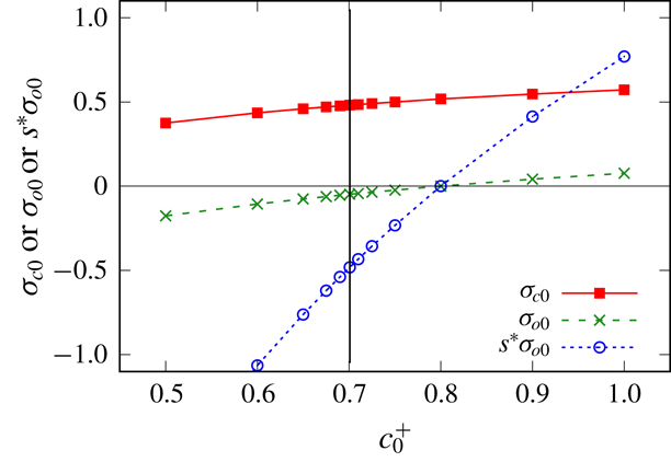
For the above parameter choices, equation (2.14) indicates that the oil is always negatively charged and in fact
 $\unicode[STIX]{x1D70E}_{o0}$
is well approximated by
 $-1/(1+{\mathcal{K}}_{o}^{1}c_{0}^{+})$
(which is the result neglecting the effect of the divalent ions). For low salinity systems in particular, with
 $c_{0}^{+}\ll 1$
, it then turns out that
 $\unicode[STIX]{x1D70E}_{o0}$
is close to
 $-1$
, and in fact for simplicity we will perform many of our calculations with
 $\unicode[STIX]{x1D70E}_{o0}$
set to
 $-1$
. The situation with
 $\unicode[STIX]{x1D70E}_{c0}$
is a little more complicated. It is evident from (2.13) that
 $\unicode[STIX]{x1D70E}_{c0}$
changes sign when
 $c_{0}^{2+}=1/{\mathcal{K}}_{c}^{2}$
. Since
 ${\mathcal{K}}_{c}^{2}=100$
here, the sign change occurs when
 $c^{2+}=0.01$
which is well within the domain of divalent ion concentrations of interest. For simplicity we will consider a number of cases with the charge state of the wall
 $\unicode[STIX]{x1D70E}_{c0}$
set to either
 $-1$
, 0 or 1, in addition to cases in which
 $\unicode[STIX]{x1D70E}_{c0}$
varies according to (2.13).
Changing the sign of
 $\unicode[STIX]{x1D70E}_{c0}$
may have a relatively limited effect, because (for the current set of Langmuir parameters) the charge on the oil
 $\unicode[STIX]{x1D70E}_{o0}$
tends to remain negative, and moreover the density of adsorption sites on the oil is rather larger than on the wall (by a factor
 $s^{\ast }=10$
). Interesting effects can however be predicted for a different set of Langmuir parameters. If the affinity of the oil for divalent ions is increased significantly such that
 ${\mathcal{K}}_{o}^{2}=25$
say (with all other Langmuir parameters remaining unchanged), then we could see sign changes for the charges on both the wall and oil, occurring respectively at divalent ion concentrations
 $c_{0}^{2+}=1/{\mathcal{K}}_{c}^{2}=0.01$
and
 $c_{0}^{2+}=1/{\mathcal{K}}_{o}^{2}=0.04$
.
For
 $c_{0}^{2+}$
between these values 0.01 and 0.04, the charges on the wall and oil are opposite in sign. If we assume a
 $c_{0}^{2+}$
:
 $c_{0}^{+}$
ratio of 1:20 (comparable with the 1:18 ratio assumed by Wilmott et al. (Reference Wilmott, Breward and Chapman2018) in their high salinity state) then for
 $c_{0}^{2+}$
very close to 0.035 (and hence
 $c_{0}^{+}$
very close to 0.7) the charges are opposite and equal, i.e.
 $\unicode[STIX]{x1D70E}_{c0}\approx -s^{\ast }\unicode[STIX]{x1D70E}_{o0}$
. In this state, the nature of the electro-osmotic term changes quite dramatically: see appendix B. Rather than having a strong disjoining tension at small distances, we have a conjoining pressure. This dramatic change in behaviour is of potential interest meaning we will analyse this case
 ${\mathcal{K}}_{o}^{2}=25$
in addition to the original situation with
 ${\mathcal{K}}_{o}^{2}=0.1$
. This clearly represents a very significant change in the affinity that the oil has for divalent ions, implying a rather different chemical composition compared to our original parameter set, but even so the assumed
 ${\mathcal{K}}_{o}^{2}=25$
for oil still remains less than
 ${\mathcal{K}}_{c}^{2}=100$
for the wall.
This completes our discussion of the methodology and parameter values to be used in the study. To summarise, our parametric studies will investigate
 $\unicode[STIX]{x1D712}^{\prime }$
values varying between 5 and 0.02,
 $\bar{\unicode[STIX]{x1D6E4}}$
values either 10 or 100 or 1000,
 $s^{\ast }=10$
, as well as
 $\unicode[STIX]{x1D70E}_{o0}=-1$
(at least in many of our calculations) along with
 $\unicode[STIX]{x1D70E}_{c0}$
either
 $-1$
, 0 or 1. In addition to this we will consider ion concentrations
 $c_{0}^{+}$
varying between 0.01 and 1, with
 $c_{0}^{2+}$
being either 0.0025 or 0.05, or else
 $c_{0}^{2+}:c_{0}^{+}$
being in a
 $1:4$
or
 $1:20$
ratio. In such cases
 $\unicode[STIX]{x1D712}^{\prime }$
,
 $\unicode[STIX]{x1D70E}_{c0}$
and
 $\unicode[STIX]{x1D70E}_{o0}$
will be determined based on the ion concentrations, with Langmuir parameters being specified, whilst
 $\bar{\unicode[STIX]{x1D6E4}}$
and
 $s^{\ast }$
remain at
 $\bar{\unicode[STIX]{x1D6E4}}=10$
and
 $s^{\ast }=10$
. Results of these parametric studies are considered in the next section.
Thickness of the aqueous film
 $J^{\ast }$
as a function of
 $\unicode[STIX]{x1D712}^{\prime }$
(the ratio between the ‘nominal’ thickness of the aqueous film and the Debye length) for various charge states: a singly charged surface (
 $\unicode[STIX]{x1D70E}_{c0}=0$
,
 $\unicode[STIX]{x1D70E}_{o0}=-1$
,
 $s^{\ast }=10$
), same sign charges (
 $\unicode[STIX]{x1D70E}_{c0}=-1$
,
 $\unicode[STIX]{x1D70E}_{o0}=-1$
,
 $s^{\ast }=10$
) and opposite but unequal charges (
 $\unicode[STIX]{x1D70E}_{c0}=1$
,
 $\unicode[STIX]{x1D70E}_{o0}=-1$
,
 $s^{\ast }=10$
). The electro-capillary parameter is
 $\bar{\unicode[STIX]{x1D6E4}}=10$
. The horizontal line indicates the Bretherton case (without electro-osmotic effects). A line proportional to
 $1/\unicode[STIX]{x1D712}^{\prime }$
is also shown to guide the eye.

4 Results
The main sets of results we consider are values of
 $J^{\ast }$
for various combinations of
 $\unicode[STIX]{x1D712}^{\prime }$
,
 $\bar{\unicode[STIX]{x1D6E4}}$
,
 $s^{\ast }$
,
 $\unicode[STIX]{x1D70E}_{c0}$
and
 $\unicode[STIX]{x1D70E}_{o0}$
(see § 4.1), and likewise values of
 $\unicode[STIX]{x0394}p^{\ast }$
for those same parameter sets (see § 4.2). After that, in § 4.3, we consider the effect of varying ion concentrations
 $c_{0}^{+}$
and
 $c_{0}^{2+}$
, whereas in § 4.4 we consider the effect of increasing the Langmuir parameter
 ${\mathcal{K}}_{o}^{2}$
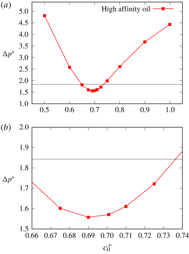
, thereby increasing the affinity of oil for adsorbing divalent ions: a key finding in § 4.4 is that
 $J^{\ast }$
and
 $\unicode[STIX]{x0394}p^{\ast }$
can vary non-monotonically with ion concentration as a result of changes in the surface charge state.
4.1 Results for film thickness
$J^{\ast }$

In what follows we consider the effect on the film thickness
 $J^{\ast }$
of varying the parameters
 $\unicode[STIX]{x1D712}^{\prime }$
(§ 4.1.1) and
 $\bar{\unicode[STIX]{x1D6E4}}$
(§ 4.1.2) for various surface charge states. The special case of opposite and equal surface charges is considered in § 4.1.3.
4.1.1 Effect of varying
$\unicode[STIX]{x1D712}^{\prime }$

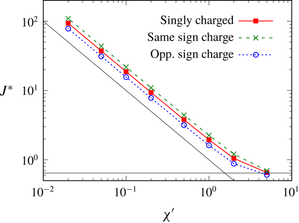
Figure 2 plots film thickness
 $J^{\ast }$
versus the parameter
 $\unicode[STIX]{x1D712}^{\prime }$
assuming
 $\bar{\unicode[STIX]{x1D6E4}}=10$
,
 $s^{\ast }=10$
, the charge state on the oil being
 $\unicode[STIX]{x1D70E}_{o0}=-1$
, and three different charge states on the wall:
 $\unicode[STIX]{x1D70E}_{c0}=0$
(a singly charged surface with charge on the oil only),
 $\unicode[STIX]{x1D70E}_{c0}=-1$
(same sign charges on the wall and oil), and
 $\unicode[STIX]{x1D70E}_{c0}=1$
(opposite but unequal charges).
When
 $\unicode[STIX]{x1D712}^{\prime }=5$
the system is close to the Bretherton state, and electrostatic effects remain weak in all cases irrespective of
 $\unicode[STIX]{x1D70E}_{c0}$
. However as
 $\unicode[STIX]{x1D712}^{\prime }$
falls, we see a significant increase in
 $J^{\ast }$
(corresponding to a significant thickening of the film). To guide the eye, a line is plotted proportional to
 $1/\unicode[STIX]{x1D712}^{\prime }$
. It would appear that
 $J^{\ast }\propto 1/\unicode[STIX]{x1D712}^{\prime }$
, or in other words
 $\unicode[STIX]{x1D712}^{\ast }\equiv J^{\ast }\unicode[STIX]{x1D712}^{\prime }$
never falls below a certain level no matter how small the value of
 $\unicode[STIX]{x1D712}^{\prime }$
. The physics behind this is clear. The film thickens so that it never explores small
 $J\,\unicode[STIX]{x1D712}^{\prime }$
values in (2.2) thereby avoiding a region in which the electro-osmotic tension would become prohibitively large. Since
 $J\,\unicode[STIX]{x1D712}^{\prime }\equiv h/\unicode[STIX]{x1D716}_{2}$
, the thinnest
 $h$
values that the film accesses are always comparable with the double layer thickness
 $\unicode[STIX]{x1D716}_{2}$
. Thus the film always benefits somewhat from charge screening. In the limit when
 $h\sim O(\unicode[STIX]{x1D716}_{2})$
and
 $\unicode[STIX]{x1D712}^{\prime }\equiv (3Ca_{B})^{2/3}/\unicode[STIX]{x1D716}_{2}\ll 1$
, it also follows (via estimating orders of magnitude of terms in (2.1)), that viscous terms are less important than capillary or electro-osmotic ones. The
 $\unicode[STIX]{x1D712}^{\prime }\ll 1$
data therefore correspond to a capillary–electrostatic limit already identified by Teletzke et al. (Reference Teletzke, Davis and Scriven1988) termed the ‘augmented Young–Laplace’ limit. Similar situations in which film thicknesses
 $h$
tend to an asymptotic value insensitive to capillary number are also observed in a related dip coating problem (Krechetnikov & Homsy Reference Krechetnikov and Homsy2005).
At any selected
 $\unicode[STIX]{x1D712}^{\prime }$
value, slight differences are seen in figure 2 between the singly charged state (charge on the oil only) and the cases with same sign charges (slightly higher disjoining tension, and hence slightly thicker films) and opposite sign charges (slightly lower disjoining tension, and hence slightly thinner films). However in all cases the charge on the oil is the dominant charge, i.e. the magnitude of
 $s^{\ast }\unicode[STIX]{x1D70E}_{o0}$
exceeds that of
 $\unicode[STIX]{x1D70E}_{c0}$
, so what happens on the wall is a small perturbation in relative terms. One interesting observation in the opposite sign charge case is that the
 $J^{\ast }$
value for
 $\unicode[STIX]{x1D712}^{\prime }=5$
is actually slightly lower than the Bretherton case (although it is difficult to see that on the scale of the graph). This follows (see appendix B) because the electro-osmotic term involving the product between the capillary wall charge and the oil charge survives out to comparatively longer distances than any other electro-osmotic term and (for opposite sign charges at comparatively large film thicknesses) now becomes a conjoining term.
4.1.2 Effect of varying
$\bar{\unicode[STIX]{x1D6E4}}$

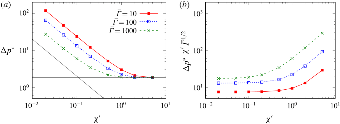
Figure 3(a) shows the effect upon
 $J^{\ast }$
versus
 $\unicode[STIX]{x1D712}^{\prime }$
of varying the parameter
 $\bar{\unicode[STIX]{x1D6E4}}$
away from the base case value
 $\bar{\unicode[STIX]{x1D6E4}}=10$
. Other parameter values are
 $\unicode[STIX]{x1D70E}_{c0}=0$
,
 $\unicode[STIX]{x1D70E}_{o0}=-1$
and
 $s^{\ast }=10$
. When
 $\bar{\unicode[STIX]{x1D6E4}}$
is larger (e.g.
 $\bar{\unicode[STIX]{x1D6E4}}=1000$
as shown here) we observe a small perturbation away from the Bretherton case, at least for
 $\unicode[STIX]{x1D712}^{\prime }\geqslant 1$
. However when
 $\unicode[STIX]{x1D712}^{\prime }$
falls below 1 (keeping
 $\bar{\unicode[STIX]{x1D6E4}}=1000$
), we still see a significant thickening of the film, with
 $J^{\ast }$
increasing proportionally to
 $1/\unicode[STIX]{x1D712}^{\prime }$
: increasing
 $J^{\ast }$
in this fashion is the only way to keep the electro-osmotic tension in check.
(a) Thickness of the aqueous film
 $J^{\ast }$
as a function of
 $\unicode[STIX]{x1D712}^{\prime }$
for three distinct values of the parameter
 $\bar{\unicode[STIX]{x1D6E4}}$
measuring the relative strength of capillary and electro-osmotic effects,
 $\bar{\unicode[STIX]{x1D6E4}}=10$
,
 $\bar{\unicode[STIX]{x1D6E4}}=100$
and
 $\bar{\unicode[STIX]{x1D6E4}}=1000$
. A singly charged surface is considered
 $\unicode[STIX]{x1D70E}_{c0}=0$
,
 $\unicode[STIX]{x1D70E}_{o0}=-1$
and
 $s^{\ast }=10$
. (b) The same data set rescaled into the form
 $J^{\ast }\,\unicode[STIX]{x1D712}^{\prime }\,\bar{\unicode[STIX]{x1D6E4}}^{1/2}$
versus
 $\unicode[STIX]{x1D712}^{\prime }$
.

 $J^{\ast }$
versus
 $\unicode[STIX]{x1D712}^{\prime }$
for the case of opposite and equal charges,
 $\unicode[STIX]{x1D70E}_{c0}=1$
,
 $\unicode[STIX]{x1D70E}_{o0}=-0.1$
,
 $s^{\ast }=10$
, with also
 $\bar{\unicode[STIX]{x1D6E4}}=10$
. The horizontal line shows the Bretherton case (without electro-osmotic effects).

Interestingly (in this small
 $\unicode[STIX]{x1D712}^{\prime }$
limit) the value of the product
 $J^{\ast }\,\unicode[STIX]{x1D712}^{\prime }$
has fallen by roughly one order of magnitude for a two order of magnitude increase in
 $\bar{\unicode[STIX]{x1D6E4}}$
. Given that the electro-osmotic term within (2.2) scales proportionally to
 $1/(\bar{\unicode[STIX]{x1D6E4}}\,(J\,\unicode[STIX]{x1D712}^{\prime })^{2})$
in the limit
 $J\,\unicode[STIX]{x1D712}^{\prime }\ll 1$
, this indicates that the system organises itself to cap the growth of the electro-osmotic tension. The implication is that
 $J^{\ast }$
is not just proportional to
 $1/\unicode[STIX]{x1D712}^{\prime }$
in the small
 $\unicode[STIX]{x1D712}^{\prime }$
limit as was identified earlier, but actually should be proportional to
 $1/(\bar{\unicode[STIX]{x1D6E4}}^{1/2}\unicode[STIX]{x1D712}^{\prime })$
. To investigate this prediction we have plotted data for an additional intermediate
 $\bar{\unicode[STIX]{x1D6E4}}$
value,
 $\bar{\unicode[STIX]{x1D6E4}}=100$
, rescaling data in figure 3(b) into the form
 $J^{\ast }\,\unicode[STIX]{x1D712}^{\prime }\,\bar{\unicode[STIX]{x1D6E4}}^{1/2}$
. In the small
 $\unicode[STIX]{x1D712}^{\prime }$
limit, we see that the rescaled data for different
 $\bar{\unicode[STIX]{x1D6E4}}$
values tend to collapse close to each other. The collapse is better for
 $\bar{\unicode[STIX]{x1D6E4}}=1000$
and
 $\bar{\unicode[STIX]{x1D6E4}}=100$
than it is for
 $\bar{\unicode[STIX]{x1D6E4}}=10$
. This is unsurprising: if
 $J^{\ast }\,\unicode[STIX]{x1D712}^{\prime }\,\bar{\unicode[STIX]{x1D6E4}}^{1/2}$
varies only very slightly with
 $\bar{\unicode[STIX]{x1D6E4}}$
, it follows that larger
 $\bar{\unicode[STIX]{x1D6E4}}$
values correspond to smaller
 $J^{\ast }\unicode[STIX]{x1D712}^{\prime }$
, and the reasoning we invoked above specifically assumed
 $J\,\unicode[STIX]{x1D712}\ll 1$
.
This then implies that, for any given
 $\bar{\unicode[STIX]{x1D6E4}}$
, the value of
 $\unicode[STIX]{x1D712}^{\prime }$
at which
 $J^{\ast }$
switches from being close to the Bretherton case (i.e.
 $J^{\ast }$
of order unity) to growing like
 $1/(\bar{\unicode[STIX]{x1D6E4}}^{1/2}\unicode[STIX]{x1D712}^{\prime })$
must itself scale like
 $\bar{\unicode[STIX]{x1D6E4}}^{-1/2}$
. In other words, the larger the value of
 $\bar{\unicode[STIX]{x1D6E4}}$
, the longer the system manages to remain close to the Bretherton system as
 $\unicode[STIX]{x1D712}^{\prime }$
is decreased.
4.1.3 Case of opposite and equal charges
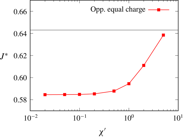
Figure 4 reverts to
 $\bar{\unicode[STIX]{x1D6E4}}=10$
but considers the case of opposite and equal charges (now with
 $\unicode[STIX]{x1D70E}_{c0}=1$
,
 $s^{\ast }=10$
and necessarily
 $\unicode[STIX]{x1D70E}_{o0}=-0.1$
in order to satisfy
 $\unicode[STIX]{x1D70E}_{c0}=-s^{\ast }\unicode[STIX]{x1D70E}_{o0}$
). As in figures 2 and 3, when
 $\unicode[STIX]{x1D712}^{\prime }=5$
, electro-osmotic effects are weak, and we see a film that is similar in thickness to the Bretherton case (Bretherton Reference Bretherton1961). However as
 $\unicode[STIX]{x1D712}^{\prime }$
decreases we now see the film becoming thinner rather than thicker: similar findings have been observed by Teletzke et al. (Reference Teletzke, Davis and Scriven1988). Nonetheless, in the case considered here, the amount of thinning is quite modest, only approximately 10 % thinner than in the Bretherton case. Unlike in the case of unequal charges (in which quite dramatic thickening of the film is required to avoid diverging electro-osmotic disjoining tensions) here, with opposite and equal charges, the electro-osmotic conjoining pressure always remains quite modest (see (B 4) in appendix B) and so only perturbs the film thickness slightly.
4.2 Results for pressure drop
$\unicode[STIX]{x0394}p^{\ast }$

This section is laid out similarly to the preceding one but considers pressure drop data
 $\unicode[STIX]{x0394}p^{\ast }$
instead of film thickness data
 $J^{\ast }$
. Specifically §§ 4.2.1–4.2.2 vary
 $\unicode[STIX]{x1D712}^{\prime }$
and
 $\bar{\unicode[STIX]{x1D6E4}}$
for various surface charge states, whereas §§ 4.2.3–4.2.4 consider the special case of opposite and equal surface charges.
4.2.1 Effect of varying
$\unicode[STIX]{x1D712}^{\prime }$

In figure 5 we plot
 $\unicode[STIX]{x0394}p^{\ast }$
(where recall that the pressure drop across the front is given by
 $\unicode[STIX]{x0394}p\equiv 1+(3Ca_{B})^{2/3}\,\unicode[STIX]{x0394}p^{\ast }$
). The parameter values considered are the same as those in figure 2. We see that
 $\unicode[STIX]{x0394}p^{\ast }$
here for
 $\unicode[STIX]{x1D712}^{\prime }=5$
is close to the Bretherton case, but as
 $\unicode[STIX]{x1D712}^{\prime }$
decreases
 $\unicode[STIX]{x0394}p^{\ast }$
is substantially larger. This is unsurprising because the aqueous film on the capillary wall is thicker, so the curvature across the front of the oil droplet must be tighter. All three cases considered (the singly charged surface, surfaces with like charges and surfaces with opposite but unequal charges) are broadly similar, but like charges lead to slightly higher
 $\unicode[STIX]{x0394}p^{\ast }$
than the singly charged case, and opposite charges lead to slightly lower
 $\unicode[STIX]{x0394}p^{\ast }$
. This is similar to what was found for the film thickness
 $J^{\ast }$
in figure 2.
The change in the driving pressure drop
 $\unicode[STIX]{x0394}p^{\ast }$
(over and above the leading-order unit capillary pressure) versus
 $\unicode[STIX]{x1D712}^{\prime }$
. The singly charged case, same sign charges and opposite but unequal charges are considered. In addition
 $\bar{\unicode[STIX]{x1D6E4}}=10$
. The horizontal line indicates the Bretherton case (without electro-osmotic effects). A line proportional to
 $1/\unicode[STIX]{x1D712}^{\prime }$
is also shown to guide the eye.

In figure 5 to guide the eye we have shown a line proportional to
 $1/\unicode[STIX]{x1D712}^{\prime }$
. It is clear that for small
 $\unicode[STIX]{x1D712}^{\prime }$
,
 $\unicode[STIX]{x0394}p^{\ast }$
is proportional to
 $1/\unicode[STIX]{x1D712}^{\prime }$
. Relative to the leading order capillary pressure drop (unity in our system), the change to the total driving pressure namely
 $(3Ca_{B})^{2/3}\unicode[STIX]{x0394}p^{\ast }$
now becomes order
 $((3Ca_{B})^{2/3})/\unicode[STIX]{x1D712}^{\prime }$
. However since
 $\unicode[STIX]{x1D712}^{\prime }$
is itself defined as
 $(3Ca_{B})^{2/3}/\unicode[STIX]{x1D716}_{2}$
, it follows that the change in the pressure drop is order
 $\unicode[STIX]{x1D716}_{2}$
roughly independently of
 $\unicode[STIX]{x1D712}^{\prime }$
.
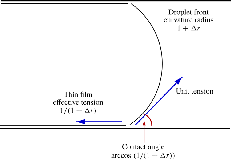
How this situation comes about can be explained as follows. In the Bretherton case,
 $(3Ca_{B})^{2/3}\unicode[STIX]{x0394}p^{\ast }$
reflects the work that must be done against viscous dissipation to drive the droplet along, over and above the interfacial tension cost associated with creating additional interface. Although not central to the argument, there is also (still in the Bretherton case) an extra contribution to
 $(3Ca_{B})^{2/3}\unicode[STIX]{x0394}p^{\ast }$
reflecting the fact that work done against interfacial tension is only done across a fraction
 $1-h^{\ast }\equiv 1-(3Ca_{B})^{2/3}J^{\ast }$
of the width of the channel, i.e. the fraction actually occupied by the droplet: the smaller the fraction of the channel over which work is performed, the larger the driving pressure needs to be to perform a given amount of work, the bulk of that work being used to create interfacial energy. In the present problem however there are two elements making up the energy cost of additional interface. First we must overcome the interfacial tension cost of creating additional interface. Then we must overcome the electro-osmotic disjoining tension associated with pushing that newly created interface towards the capillary wall.
In the limit of small
 $\unicode[STIX]{x1D712}^{\prime }$
(which is also the limit of small
 $Ca_{B}$
since
 $\unicode[STIX]{x1D712}^{\prime }=(3Ca_{B})^{2/3}/\unicode[STIX]{x1D716}_{2}$
) the work done against disjoining tension considerably exceeds that done against viscous dissipation. If the viscous effects are thereby neglected, energetically we have capillary–electrostatic problem (the augmented Young–Laplace limit of Teletzke et al. (Reference Teletzke, Davis and Scriven1988)): the ‘effective’ interfacial tension of the thin film (i.e. actual energy cost per unit area of film including the electro-osmotic effect) exceeds the ‘raw’ interfacial tension (without electro-osmotic effects). It is this ‘effective’ interfacial tension which contributes to a higher energy cost (and hence a higher driving pressure) as the droplet displaces along.
The work done against the electro-osmotic tension is obtained from
 $\bar{\unicode[STIX]{x1D6E4}}^{-1}\int _{h}^{\infty }T_{EO}\,\text{d}h$
. Extracting the electro-osmotic term from (2.1) and integrating yields
 $$\begin{eqnarray}\displaystyle \int _{h}^{\infty }T_{EO}\,\text{d}h & = & \displaystyle 2\unicode[STIX]{x1D70E}_{c0}^{2}\unicode[STIX]{x1D716}_{2}\exp (-2h/\unicode[STIX]{x1D716}_{2})/(1-\exp (-2h/\unicode[STIX]{x1D716}_{2}))\nonumber\\ \displaystyle & & \displaystyle +\,2s^{\ast }\unicode[STIX]{x1D70E}_{c0}\unicode[STIX]{x1D70E}_{o0}\unicode[STIX]{x1D716}_{2}/\sinh (h/\unicode[STIX]{x1D716}_{2})\nonumber\\ \displaystyle & & \displaystyle +\,2s^{\ast \,2}\unicode[STIX]{x1D70E}_{o0}^{2}\unicode[STIX]{x1D716}_{2}\exp (-2h/\unicode[STIX]{x1D716}_{2})/(1-\exp (-2h/\unicode[STIX]{x1D716}_{2})).\end{eqnarray}$$
The lower limit of integration for (4.1) is not given a priori, since that depends upon how thin the film becomes (and that also depends on
 $\bar{\unicode[STIX]{x1D6E4}}$
). However we know from figure 3 that, in the small
 $\unicode[STIX]{x1D712}^{\prime }$
limit,
 $J^{\ast }\,\unicode[STIX]{x1D712}^{\prime }$
is roughly constant for any given
 $\bar{\unicode[STIX]{x1D6E4}}$
: since
 $J\,\unicode[STIX]{x1D712}^{\prime }\equiv h/\unicode[STIX]{x1D716}_{2}$
, the film thickness
 $h$
never falls below order
 $\unicode[STIX]{x1D716}_{2}$
. Under those circumstances equation (4.1) predicts a value that is order
 $\unicode[STIX]{x1D716}_{2}$
, agreeing with our earlier claim that the change in the pressure drop due to electro-osmotic effects should likewise be order
 $\unicode[STIX]{x1D716}_{2}$
.
4.2.2 Effect of varying
$\bar{\unicode[STIX]{x1D6E4}}$

The previous subsection examined how
 $\unicode[STIX]{x0394}p^{\ast }$
varied with
 $\unicode[STIX]{x1D712}^{\prime }$
for a fixed
 $\bar{\unicode[STIX]{x1D6E4}}$
. However
 $\unicode[STIX]{x0394}p^{\ast }$
also depends on
 $\bar{\unicode[STIX]{x1D6E4}}$
as is seen in figure 6 by comparing data for
 $\bar{\unicode[STIX]{x1D6E4}}=10$
with data for
 $\bar{\unicode[STIX]{x1D6E4}}=100$
and
 $\bar{\unicode[STIX]{x1D6E4}}=1000$
. Values of
 $\unicode[STIX]{x1D70E}_{c0}$
,
 $s^{\ast }$
and
 $\unicode[STIX]{x1D70E}_{o0}$
are as per figure 3. Qualitatively the
 $\unicode[STIX]{x0394}p^{\ast }$
data in figure 6(a) follow the same trends as
 $J^{\ast }$
data in figure 3(a). Data for
 $\bar{\unicode[STIX]{x1D6E4}}=1000$
stay closer to the Bretherton data for longer as
 $\unicode[STIX]{x1D712}^{\prime }$
decreases, and for each
 $\bar{\unicode[STIX]{x1D6E4}}$
the data scale like
 $1/\unicode[STIX]{x1D712}^{\prime }$
for small
 $\unicode[STIX]{x1D712}^{\prime }$
. In this small
 $\unicode[STIX]{x1D712}^{\prime }$
limit, a two order of magnitude increase in
 $\bar{\unicode[STIX]{x1D6E4}}$
leads to roughly a single order of magnitude decrease in
 $\unicode[STIX]{x0394}p^{\ast }$
, again analogous to what is seen for
 $J^{\ast }$
in figure 3. In figure 6(b) we aim to collapse data with different
 $\bar{\unicode[STIX]{x1D6E4}}$
by plotting
 $\unicode[STIX]{x0394}p^{\ast }\,\unicode[STIX]{x1D712}^{\prime }\,\bar{\unicode[STIX]{x1D6E4}}^{1/2}$
versus
 $\unicode[STIX]{x1D712}^{\prime }$
. Although the collapse is not as good as seen in figure 3(b), we again see the tendency towards better collapse with increasing
 $\bar{\unicode[STIX]{x1D6E4}}$
value.
(a) Pressure drop
 $\unicode[STIX]{x0394}p^{\ast }$
versus
 $\unicode[STIX]{x1D712}^{\prime }$
for three distinct values of the parameter
 $\bar{\unicode[STIX]{x1D6E4}}$
, namely
 $\bar{\unicode[STIX]{x1D6E4}}=10$
,
 $\bar{\unicode[STIX]{x1D6E4}}=100$
and
 $\bar{\unicode[STIX]{x1D6E4}}=1000$
. A singly charged surface is considered. (b) The same data set rescaled into the form
 $\unicode[STIX]{x0394}p^{\ast }\,\unicode[STIX]{x1D712}^{\prime }\,\bar{\unicode[STIX]{x1D6E4}}^{1/2}$
versus
 $\unicode[STIX]{x1D712}^{\prime }$
.

4.2.3 Case of opposite and equal charges
In the case of opposite and equal charges
 $\unicode[STIX]{x1D70E}_{c0}=-s^{\ast }\unicode[STIX]{x1D70E}_{o0}$
(with parameter values chosen as per figure 4) we have plotted
 $\unicode[STIX]{x0394}p^{\ast }$
versus
 $\unicode[STIX]{x1D712}^{\prime }$
: see figure 7. Unsurprisingly the
 $\unicode[STIX]{x0394}p^{\ast }$
values tend to be smaller than for the Bretherton case. The film is now slightly thinner than the Bretherton film, so the curvature radius of the droplet front can be slightly larger, and this is associated with a decrease in
 $\unicode[STIX]{x0394}p^{\ast }$
. A surprise happens however when
 $\unicode[STIX]{x1D712}^{\prime }$
becomes sufficiently small, namely
 $\unicode[STIX]{x0394}p^{\ast }$
switches sign. For these parameter values (
 $\bar{\unicode[STIX]{x1D6E4}}=10$
,
 $\unicode[STIX]{x1D70E}_{c0}=1$
,
 $\unicode[STIX]{x1D70E}_{o0}=-0.1$
and
 $s^{\ast }=10$
) this switch is observed to happen when
 $\unicode[STIX]{x1D712}^{\prime }$
is approximately 0.1.
Pressure drop
 $\unicode[STIX]{x0394}p^{\ast }$
versus
 $\unicode[STIX]{x1D712}^{\prime }$
for the case of opposite and equal charges, with also
 $\bar{\unicode[STIX]{x1D6E4}}=10$
. The horizontal line indicates the Bretherton case (without electro-osmotic effects).

The sign change in
 $\unicode[STIX]{x0394}p^{\ast }$
can be understood as follows. Remember that the total driving pressure
 $\unicode[STIX]{x0394}p=1+(3Ca_{B})^{2/3}\unicode[STIX]{x0394}p^{\ast }$
is comprised of a leading-order capillary static term, plus corrections from viscous and electro-osmotic terms, as well as an additional correction (see § 4.2.1) reflecting the fact that work is only done by the pressure across the fraction of the channel width actually occupied by the drop. In the present case with opposite and equal charges on the oil and the wall, work is actually doneby the electro-osmotic conjoining pressure (rather than being done against a disjoining tension). For small enough
 $\unicode[STIX]{x1D712}^{\prime }$
, it appears that the work done by the electro-osmotic conjoining pressure actually exceeds the energy lost to viscous dissipation (plus the additional correction due to displacing through just a fraction of the channel width), so it is slightly easier to push the oil droplet along than would be determined by considering capillary effects alone.
Over the
 $\unicode[STIX]{x1D712}^{\prime }$
domain studied here, which (see § 3.2) corresponds to the likely domain of interest in waterflooding applications, it is much less clear (compared to the case in § 4.2.1) that
 $\unicode[STIX]{x0394}p^{\ast }$
exhibits a scaling proportional to
 $1/\unicode[STIX]{x1D712}^{\prime }$
at small
 $\unicode[STIX]{x1D712}^{\prime }$
, although such a scaling is plausible. Recall that in § 4.2.1 we argued that this scaling implied a pressure change
 $(3Ca_{B})^{2/3}\unicode[STIX]{x0394}p^{\ast }$
of the order of
 $\unicode[STIX]{x1D716}_{2}$
(regardless of the value of
 $\unicode[STIX]{x1D712}^{\prime }$
) and this came about when
 $\unicode[STIX]{x0394}p^{\ast }$
was dominated by an electro-osmotic work contribution. The ‘effective’ interfacial tension in such a system can be evaluated as the ‘raw’ tension less the amount of work done by the electro-osmotic pressure as
 $h$
decreases. This amount of work can be estimated as
 $\bar{\unicode[STIX]{x1D6E4}}^{-1}\int _{h}^{\infty }p_{EO}\,\text{d}h$
where
 $$\begin{eqnarray}\displaystyle \int _{h}^{\infty }p_{EO}\,\text{d}h=2|s^{\ast }\unicode[STIX]{x1D70E}_{c0}\unicode[STIX]{x1D70E}_{o0}|\,2\unicode[STIX]{x1D716}_{2}(\exp (-h/\unicode[STIX]{x1D716}_{2})-\exp (-2h/\unicode[STIX]{x1D716}_{2}))/(1-\exp (-2h/\unicode[STIX]{x1D716}_{2})). & & \displaystyle\end{eqnarray}$$
The limiting value of this for
 $h\ll \unicode[STIX]{x1D716}_{2}$
is
 $2|s^{\ast }\unicode[STIX]{x1D70E}_{c0}\unicode[STIX]{x1D70E}_{o0}|\unicode[STIX]{x1D716}_{2}$
, which does indeed give a value of order
 $\unicode[STIX]{x1D716}_{2}$
as anticipated. The difficulty we face here (compared to § 4.2.1) is that in the present system the work done by electro-osmotic pressures is offset by work done against viscous forces, and since films thin here (rather than thicken) as
 $\unicode[STIX]{x1D712}^{\prime }$
decreases, it is less easy to justify neglect of those viscous forces.
4.2.4 Implications for contact angles
The fact that the ‘effective’ interfacial tension can be less than the ‘raw’ tension has an important implication when the system is viewed macroscopically with a uniformly curved drop front joining up with a thin film along the capillary wall. The situation is sketched in figure 8. Since the total pressure drop is now
 $1-(3Ca_{B})^{2/3}|\unicode[STIX]{x0394}p^{\ast }|$
and so is less than unity, the curvature radius of the front (i.e. the reciprocal of the total pressure drop) is greater than unity. In the space available across the half-thickness of the channel, the droplet front can no longer curve sufficiently to meet the capillary wall tangentially. Denoting the curvature radius by
 $1+\unicode[STIX]{x0394}r$
, with
 $\unicode[STIX]{x0394}r\approx (3Ca_{B})^{2/3}|\unicode[STIX]{x0394}p^{\ast }|\ll 1$
, the front turns through an angle
 $\arcsin (1/(1+\unicode[STIX]{x0394}r))$
across the half-thickness, meaning that it meets the capillary wall at a contact angle
 $\unicode[STIX]{x03C0}/2-\arcsin (1/(1+\unicode[STIX]{x0394}r))=\arccos (1/(1+\unicode[STIX]{x0394}r))$
. Systems such as these with finite (apparent) contact angles have been considered already by Teletzke et al. (Reference Teletzke, Davis and Scriven1988), Krechetnikov & Homsy (Reference Krechetnikov and Homsy2005), Cox et al. (Reference Cox, Kraynik, Weaire and Hutzler2018).
A macroscopic view of a situation in which the effective interfacial tension on the thin film at the capillary wall is less than the interfacial tension on the droplet front. The radius of curvature of the droplet front is greater than unity (unity is the half-distance between the capillary walls), and the curved front appears to meet the capillary wall at a finite contact angle.

Local force balance at the contact point, requires us to balance the ‘raw’ interfacial tension force on the droplet front projected onto the capillary wall, with the weaker ‘effective’ interfacial tension force in the thin film. The projection involves the cosine of the contact angle which evaluates to
 $1/(1+\unicode[STIX]{x0394}r)$
. This is however exactly the ‘effective’ interfacial tension. The work done to advance the front per unit of distance is determined by the imposed pressure
 $1/(1+\unicode[STIX]{x0394}r)$
and this work done is reflected in the energy per unit area of thin film created, which is nothing other than the aforementioned ‘effective’ tension. Thus a front driven along by a total pressure less than unity, is (at least in a capillary–electrostatic system) entirely consistent with an ‘effective’ interfacial film tension less than the raw tension, leading to a finite contact angle at the capillary wall.
4.3 Effect of varying ion concentrations
$c_{0}^{+}$
and
$c_{0}^{2+}$


Whereas previously in §§ 4.1–4.2 we considered varying
 $\unicode[STIX]{x1D712}^{\prime }$
values for a given surface charge state (which physically could be achieved by moving an oil droplet at a different speed), here we consider varying
 $\unicode[STIX]{x1D712}^{\prime }$
by varying ion concentrations
 $c_{0}^{+}$
and
 $c_{0}^{2+}$
. As we shall see, this has the side effect of varying surface charges (§ 4.3.1) in addition to affecting film thickness
 $J^{\ast }$
and pressure drop
 $\unicode[STIX]{x0394}p^{\ast }$
(§§ 4.3.2–4.3.3).
4.3.1 Effect upon surface charges
$\unicode[STIX]{x1D70E}_{c0}$
and
$\unicode[STIX]{x1D70E}_{o0}$


All data examined thus far varied
 $\unicode[STIX]{x1D712}^{\prime }$
with the charges per adsorption site (
 $\unicode[STIX]{x1D70E}_{c0}$
and
 $\unicode[STIX]{x1D70E}_{o0}$
) fixed. Here however we vary
 $\unicode[STIX]{x1D712}^{\prime }$
by varying ion concentrations, which affects
 $\unicode[STIX]{x1D70E}_{c0}$
and
 $\unicode[STIX]{x1D70E}_{o0}$
. Remember from § 3.2 that a
 $\unicode[STIX]{x1D712}^{\prime }$
value of 0.22 (or roughly speaking 0.2) along with a
 $c_{0}^{+}$
value of order unity would be typical for a high salinity case, and moreover (from §§ 2.3 and 3.3) that
 $\unicode[STIX]{x1D712}^{\prime }\propto (c_{0}^{+})^{1/2}$
(which applies as long as monovalent ions are more plentiful than divalent ones). We suppose
 $\unicode[STIX]{x1D712}^{\prime }=0.2\,(c_{0}^{+})^{1/2}$
and we consider a range of
 $c_{0}^{+}$
values from unity (high salinity) down to 0.01 (low salinity).
A side effect of changing
 $c_{0}^{+}$
however is that
 $\unicode[STIX]{x1D70E}_{c0}$
and
 $\unicode[STIX]{x1D70E}_{o0}$
must also change. An example of how these quantities change versus monovalent ion concentration
 $c^{+}$
is plotted in figure 9. Within this figure, we consider 3 separate sets of divalent ion concentrations as per § 3.3: a low divalent ion concentration (
 $c_{0}^{2+}=0.0025$
, comparable with what is assumed in the low salinity state of Wilmott et al. (Reference Wilmott, Breward and Chapman2018)), a high divalent ion concentration (
 $c_{0}^{2+}=0.05$
, comparable with the high salinity state of Wilmott et al. (Reference Wilmott, Breward and Chapman2018)), and a fixed ratio between divalent:monovalent ions (a 1:4 ratio comparable with the ratio assumed in the low salinity state of Wilmott et al. (Reference Wilmott, Breward and Chapman2018)).
Charge on the capillary wall
 $\unicode[STIX]{x1D70E}_{c0}$
or the oil
 $\unicode[STIX]{x1D70E}_{o0}$
versus salinity
 $c_{0}^{+}$
(monovalent ion concentration). Langmuir parameters are
 ${\mathcal{K}}_{c}^{1}=1$
,
 ${\mathcal{K}}_{c}^{2}=100$
,
 ${\mathcal{K}}_{o}^{1}=1$
,
 ${\mathcal{K}}_{o}^{2}=0.1$
. For
 $\unicode[STIX]{x1D70E}_{c0}$
three different divalent ion concentrations are considered, low concentration (
 $c_{0}^{2+}=0.0025$
, squares), higher concentration (
 $c_{0}^{2+}=0.05$
, crosses) and a fixed divalent: monovalent ratio of 1:4 (circles). For
 $\unicode[STIX]{x1D70E}_{o0}$
only the fixed divalent:monovalent ratio is plotted (solid line), but results are very insensitive to the divalent ion concentration (owing to the parameter
 ${\mathcal{K}}_{o}^{2}$
being small).

We see in figure 9 that for low divalent ion concentrations, the charge per adsorption site on the the wall
 $\unicode[STIX]{x1D70E}_{c0}$
is negative, whereas for high divalent ion concentrations
 $\unicode[STIX]{x1D70E}_{c0}$
is positive, and for a fixed monovalent:divalent concentration ratio
 $\unicode[STIX]{x1D70E}_{c0}$
switches between negative and positive as
 $c_{0}^{+}$
changes. Equation (2.13) indicates that what controls the sign of
 $\unicode[STIX]{x1D70E}_{c0}$
is the adsorption of divalent ions, and the wall’s strong affinity for divalent ions (the Langmuir constant being
 ${\mathcal{K}}_{c}^{2}=100$
) makes these sign changes possible. The sign change occurs when
 ${\mathcal{K}}_{c}^{2}c_{0}^{2+}=1$
corresponding to
 $c_{0}^{2+}=0.01$
for our data, and hence
 $c_{0}^{+}=0.04$
(divalent:monovalent ions are kept in a 1:4 ratio for the data set in question).
Considering now the oil rather than the wall, we note that the Langmuir constant for adsorption of divalent ions onto oil
 ${\mathcal{K}}_{o}^{2}$
is very small, namely
 ${\mathcal{K}}_{o}^{2}=0.1$
. As a result
 $\unicode[STIX]{x1D70E}_{o0}$
is always negative, making (2.14) very insensitive to
 $c_{0}^{2+}$
, and hence insensitive to whether we consider the low divalent ion case, the high divalent ion case or the fixed monovalent:divalent ion ratio. Indeed as already mentioned in § 3.3, to a good approximation,
 $\unicode[STIX]{x1D70E}_{o0}\approx -1/(1+{\mathcal{K}}_{o}^{1}c_{0}^{+})$
, where recall
 ${\mathcal{K}}_{o}^{1}=1$
. This means that as
 $c_{0}^{+}$
falls from
 $c_{0}^{+}=1$
to
 $c_{0}^{+}\ll 1$
,
 $\unicode[STIX]{x1D70E}_{o0}$
becomes more negative and roughly doubles in magnitude.
4.3.2 Effect upon film thickness
$J^{\ast }$

Having now obtained values of
 $\unicode[STIX]{x1D70E}_{c0}$
and
 $\unicode[STIX]{x1D70E}_{o0}$
, in figure 10(a) we show data for film thickness
 $J^{\ast }$
versus
 $c_{0}^{+}$
. Parameter values are as per figure 9 with also
 $\bar{\unicode[STIX]{x1D6E4}}=10$
and
 $s^{\ast }=10$
. The first set of data we examine is for the low divalent ion concentration system (
 $c_{0}^{2+}=0.0025$
). The main effect we see is that
 $J^{\ast }$
increases as
 $c_{0}^{+}$
increases. To guide the eye we have plotted a line proportional to
 $(c_{0}^{+})^{-1/2}$
: owing to the square root relationship between
 $\unicode[STIX]{x1D712}^{\prime }$
and
 $c_{0}^{+}$
, this corresponds to a line proportional to
 $1/\unicode[STIX]{x1D712}^{\prime }$
, as was plotted in figure 2. For smaller
 $c_{0}^{+}$
values the data are parallel to this line, but if we start from
 $c_{0}^{+}$
close to 1, and then decrease
 $c_{0}^{+}$
, the
 $J^{\ast }$
data rise faster than the line does. The effect we are seeing here is the increase in the magnitude of the charge on the oil
 $\unicode[STIX]{x1D70E}_{o0}$
as
 $c_{0}^{+}$
falls.
(a) Film thickness
 $J^{\ast }$
versus
 $c_{0}^{+}$
, assuming
 $\unicode[STIX]{x1D712}^{\prime }=0.2\,(c_{0}^{+})^{1/2}$
but also allowing
 $\unicode[STIX]{x1D70E}_{c0}$
and
 $\unicode[STIX]{x1D70E}_{o0}$
to vary with
 $c_{0}^{+}$
. Divalent ion concentrations are set as either low (
 $c_{0}^{2+}=0.0025$
), high (
 $c_{0}^{2+}=0.05$
), or in a fixed divalent:monovalent ratio of 1:4. In addition
 $\bar{\unicode[STIX]{x1D6E4}}=10$
and
 $s^{\ast }=10$
. A line proportional to
 $(c_{0}^{+})^{-1/2}$
is shown to guide the eye. (b) Pressure drop
 $\unicode[STIX]{x0394}p^{\ast }$
versus
 $c_{0}^{+}$
.

Data for
 $J^{\ast }$
versus
 $c_{0}^{+}$
for a much higher divalent ion concentration (
 $c_{0}^{2+}=0.05$
) are also considered. The behaviour of the predicted
 $J^{\ast }$
values mirrors what is discussed above in the low divalent ion concentration case (
 $c_{0}^{2+}=0.0025$
). However
 $J^{\ast }$
values are now shifted to lower values. This is due to the sign of
 $\unicode[STIX]{x1D70E}_{c0}$
having changed. In the previous case when
 $c_{0}^{2+}=0.0025$
,
 $\unicode[STIX]{x1D70E}_{c0}$
is negative and so has the same sign as
 $\unicode[STIX]{x1D70E}_{o0}$
. However when
 $c_{0}^{2+}=0.05$
,
 $\unicode[STIX]{x1D70E}_{c0}$
has become positive, opposite in sign from
 $\unicode[STIX]{x1D70E}_{o0}$
, leading to slightly thinner films than before, i.e. slightly smaller
 $J^{\ast }$
. The effect of changing the sign of the charge on the wall remains however a relatively small one, because the oil still has a much bigger overall charge than the wall, having many more adsorption sites available (i.e.
 $s^{\ast }=10$
).
The final case in figure 10(a) varies overall ion concentration but holds the ratio between divalent and monovalent ions fixed at 1:4. For these data as
 $c_{0}^{+}$
decreases,
 $J^{\ast }$
rises more rapidly than
 $(c_{0}^{+})^{-1/2}$
, i.e. more rapidly than
 $1/\unicode[STIX]{x1D712}^{\prime }$
. The reason is that reducing
 $c_{0}^{+}$
not only causes
 $\unicode[STIX]{x1D712}^{\prime }$
to fall, but also causes
 $\unicode[STIX]{x1D70E}_{c0}$
to switch sign, from positive (opposite in sign from
 $\unicode[STIX]{x1D70E}_{o0}$
) to negative (the same sign as
 $\unicode[STIX]{x1D70E}_{o0}$
): that causes the film to thicken.
4.3.3 Effect upon pressure drop
$\unicode[STIX]{x0394}p^{\ast }$

Figure 10(b) shows data for
 $\unicode[STIX]{x0394}p^{\ast }$
versus
 $c_{0}^{+}$
for the same set of conditions as in figure 10(a). Qualitatively the results in the two figures are very similar. As
 $c_{0}^{+}$
falls at fixed divalent ion concentration,
 $\unicode[STIX]{x0394}p^{\ast }$
grows slightly faster than
 $(c_{0}^{+})^{-1/2}$
reflecting a growth in the magnitude of
 $\unicode[STIX]{x1D70E}_{o0}$
in addition to a reduction in
 $\unicode[STIX]{x1D712}^{\prime }$
. At any given monovalent ion concentration
 $c_{0}^{+}$
, higher divalent ion concentrations, for which the oil and wall are oppositely charged, give lower
 $\unicode[STIX]{x0394}p^{\ast }$
than low divalent ion concentrations, for which the oil and wall have like charges. Reducing
 $c_{0}^{+}$
at a specified
 $c_{0}^{2+}$
:
 $c_{0}^{+}$
ion ratio leads to greater increases in
 $\unicode[STIX]{x0394}p^{\ast }$
than would be observed for any fixed
 $c_{0}^{2+}$
value, this being due to a change in sign of
 $\unicode[STIX]{x1D70E}_{c0}$
as
 $c_{0}^{+}$
decreases when
 $c_{0}^{+}$
and
 $c_{0}^{2+}$
are held at a specified ratio. The surface of the wall thereby switches from being oppositely charged from the oil to having a like charge.
Values of surface charges
 $\unicode[STIX]{x1D70E}_{c0}$
,
 $\unicode[STIX]{x1D70E}_{o0}$
and
 $s^{\ast }\unicode[STIX]{x1D70E}_{o0}$
versus monovalent ion concentration
 $c_{0}^{+}$
. Here
 $s^{\ast }=10$
and the Langmuir constants are
 ${\mathcal{K}}_{c}^{1}=1$
,
 ${\mathcal{K}}_{c}^{1}=100$
,
 ${\mathcal{K}}_{o}^{1}=1$
and
 ${\mathcal{K}}_{o}^{2}=25$
, and we consider a ratio of divalent:monovalent ion concentrations of 1:20. The vertical line indicates the
 $c_{0}^{+}$
value giving the opposite and equal charged case namely
 $\unicode[STIX]{x1D70E}_{c0}=-s^{\ast }\unicode[STIX]{x1D70E}_{o0}$
.

4.4 Case with a large
${\mathcal{K}}_{o}^{2}$

In §§ 4.1.3 and 4.2.3 we saw that the system exhibits quite distinctive behaviours when surface charges
 $\unicode[STIX]{x1D70E}_{c0}$
and
 $s^{\ast }\unicode[STIX]{x1D70E}_{o0}$
become opposite and equal. In principle such a state can be achieved by varying concentrations,
 $c_{0}^{+}$
and
 $c_{0}^{2+}$
. In practice however this did not happen in § 4.3 because the value of the Langmuir parameter
 ${\mathcal{K}}_{o}^{2}$
was such that very few divalent ions adsorbed on the oil in the concentration range of interest. This limited the variation of
 $\unicode[STIX]{x1D70E}_{o0}$
away from
 $-1$
, and since
 $s^{\ast }$
was also significantly larger than unity, the charge on the oil tended to overwhelm that on the wall. Here we investigate a case with a much larger
 ${\mathcal{K}}_{o}^{2}$
, exploring the effects on the surface charges (§ 4.4.1), as well as on film thickness
 $J^{\ast }$
(§ 4.4.2) and pressure drop
 $\unicode[STIX]{x0394}p^{\ast }$
(§ 4.4.3). As we will see,
 $J^{\ast }$
and
 $\unicode[STIX]{x0394}p^{\ast }$
can exhibit non-monotonic behaviour as
 $c_{0}^{+}$
and
 $c_{0}^{2+}$
vary.
4.4.1 Effect upon surface charges
$\unicode[STIX]{x1D70E}_{c0}$
and
$\unicode[STIX]{x1D70E}_{o0}$


Here we suppose that
 ${\mathcal{K}}_{o}^{2}=25$
(much higher than the value
 ${\mathcal{K}}_{o}^{2}=0.1$
considered previously, but still significantly less than the analogous parameter for the wall
 ${\mathcal{K}}_{c}^{2}$
which equals 100). We assume moreover that the divalent and monovalent ion concentrations are in a 1:20 ratio (a ratio comparable with what Wilmott et al. (Reference Wilmott, Breward and Chapman2018) assumed in their high salinity case). Data for the surface charges
 $\unicode[STIX]{x1D70E}_{c0}$
and
 $\unicode[STIX]{x1D70E}_{o0}$
are plotted in figure 11. Both
 $\unicode[STIX]{x1D70E}_{c0}$
and
 $\unicode[STIX]{x1D70E}_{o0}$
now change sign as the ion concentration
 $c_{0}^{+}$
varies. However these sign changes do not happen at the same
 $c_{0}^{+}$
. In fact
 $\unicode[STIX]{x1D70E}_{c0}$
switches sign when
 $c_{0}^{+}=0.2$
(i.e.
 $c_{0}^{2+}=0.01$
) whereas
 $\unicode[STIX]{x1D70E}_{o0}$
switches sign when
 $c_{0}^{+}=0.8$
(i.e.
 $c_{0}^{2+}=0.04$
). For
 $0.2<c_{0}^{+}<0.8$
therefore, the values of
 $\unicode[STIX]{x1D70E}_{c0}$
and
 $\unicode[STIX]{x1D70E}_{o0}$
are of opposite sign, and it turns out there is a particular value of
 $c_{0}^{+}$
very close to
 $c_{0}^{+}\approx 0.7$
(see figure 11) at which the charges become opposite and equal, i.e.
 $\unicode[STIX]{x1D70E}_{c0}=-s^{\ast }\unicode[STIX]{x1D70E}_{o0}$
(assuming
 $s^{\ast }=10$
).
4.4.2 Effect upon film thickness
$J^{\ast }$

In figure 12 we show results for film thickness
 $J^{\ast }$
sweeping through concentration values
 $c_{0}^{+}$
from
 $c_{0}^{+}=1$
down to
 $c_{0}^{+}=0.5$
. Parameter values are as per figure 11 with in addition
 $\bar{\unicode[STIX]{x1D6E4}}=10$
. Instead of a conventional picture in which
 $J^{\ast }$
increases as
 $c_{0}^{+}$
decreases, the system is now strongly affected by the charge state of the surfaces, with the film thickness
 $J^{\ast }$
falling to a minimum at the point where charges are opposite and equal (very close to
 $c_{0}^{+}=0.7$
). As is seen in the zoomed view in figure 12(b), the film thickness
 $J^{\ast }$
at this minimum is actually smaller than the Bretherton case (Bretherton Reference Bretherton1961).
(a) Film thickness
 $J^{\ast }$
versus ion concentration
 $c_{0}^{+}$
. It is assumed that
 $\unicode[STIX]{x1D712}^{\prime }=0.2\,(c_{0}^{+})^{1/2}$
,
 $\bar{\unicode[STIX]{x1D6E4}}=10$
and values of
 $\unicode[STIX]{x1D70E}_{c0}$
and
 $s^{\ast }\unicode[STIX]{x1D70E}_{o0}$
are as per figure 11. The horizontal line represents the Bretherton case. (b) Zoomed view.

4.4.3 Effect upon pressure drop
$\unicode[STIX]{x0394}p^{\ast }$

Analogous data for
 $\unicode[STIX]{x0394}p^{\ast }$
versus
 $c_{0}^{+}$
are presented in figure 13. Again instead of the conventional picture in which
 $\unicode[STIX]{x0394}p^{\ast }$
grows as
 $c_{0}^{+}$
falls, we see that
 $\unicode[STIX]{x0394}p^{\ast }$
falls to a minimum owing to the changes in the charge state of the surfaces. In the zoomed view figure 13(b) we observe that
 $\unicode[STIX]{x0394}p^{\ast }$
falls below the Bretherton equivalent. Recall from § 4.2.3 that we correlated falling values of
 $\unicode[STIX]{x0394}p^{\ast }$
with work done by the electro-osmotic conjoining pressure which can help the droplet front to move along. Unlike what was seen in figure 7, here in figure 13,
 $\unicode[STIX]{x0394}p^{\ast }$
never becomes negative: whilst work can be done by the conjoining pressure, it fails to match the positive contributions to
 $\unicode[STIX]{x0394}p^{\ast }$
arising from viscous dissipation losses plus other effects (a pressure increase is needed to compensate for displacement only occurring across a fraction of the channel width as per § 4.2.1).
(a) Pressure drop
 $\unicode[STIX]{x0394}p^{\ast }$
versus ion concentration
 $c_{0}^{+}$
. Parameter values are as per figure 12 and the horizontal line represents the Bretherton case. (b) Zoomed view.

One interesting feature of figure 13 (a contrast with what is found for
 $J^{\ast }$
in figure 12) is that the local minimum for
 $\unicode[STIX]{x0394}p^{\ast }$
appears to occur around
 $c_{0}^{+}\approx 0.69$
and so does not coincide with the point of opposite and equal charges which is known to occur at a
 $c_{0}^{+}$
value extremely close to 0.7. Recall (see § 3.1 and also appendix C) that there is more uncertainty in predicted
 $\unicode[STIX]{x0394}p^{\ast }$
values than in
 $J^{\ast }$
values owing to slower convergence. That notwithstanding, the very slight decrease in
 $\unicode[STIX]{x0394}p^{\ast }$
when decreasing
 $c_{0}^{+}$
slightly below 0.7 can also be explained by the nature of the conjoining and disjoining terms for charges that are nearly (but not quite) opposite and equal: details are given in appendix D.
5 Discussion and conclusions
In the context of oil recovery operations, a model for a charged droplet moving along a charged capillary channel has been considered, based on work by Wilmott et al. (Reference Wilmott, Breward and Chapman2018) providing an extension of classical results (for the uncharged case) of Bretherton (Reference Bretherton1961). The governing equations of the model contain not only the capillary and viscous terms considered by Bretherton but also an additional electro-osmotic term. In the interests of simplicity, we have focussed attention solely on the front part of the droplet, ignoring what happens at the rear (despite the fact that Wilmott et al. (Reference Wilmott, Breward and Chapman2018) indicated that interesting effects could also be observed at the rear).
One of the key dimensionless parameters governing the system behaviour is
 $\unicode[STIX]{x1D712}^{\prime }$
which is the ratio between the ‘nominal’ thickness of the aqueous layer separating the droplet from the capillary wall and the thickness of the electrical double layer (the Debye length). The ‘nominal’ thickness here is what would be predicted by Bretherton (Reference Bretherton1961) ignoring electrostatic effects (and is proportional to
 $(3Ca_{B})^{2/3}$
where
 $Ca_{B}$
is a capillary number). When
 $\unicode[STIX]{x1D712}^{\prime }$
is large, electrostatic effects are strongly screened and Bretherton’s results are recovered (Bretherton Reference Bretherton1961). However when
 $\unicode[STIX]{x1D712}^{\prime }$
is small, significant departures from Bretherton’s results are found. Corroborating findings by Teletzke et al. (Reference Teletzke, Davis and Scriven1988), the aqueous layer then becomes much thicker than Bretherton’s ‘nominal’ value (by an amount proportional to
 $1/\unicode[STIX]{x1D712}^{\prime }$
) and in fact keeps itself of comparable thickness with the electrical double layer, so that electrostatic effects manage to be screened to some extent. The pressure needed to drive the oil droplet front along consists of a capillary pressure plus corrections due to viscous dissipation and due to work being done across just part of the channel (as already identified by Bretherton (Reference Bretherton1961)) plus an additional new correction due to work done against an electro-osmotic tension. In the limit of very small
 $\unicode[STIX]{x1D712}^{\prime }$
, the electro-osmotic correction seems to dominate the viscous one, suggesting that a capillary–electrostatic limit has been reached (the so called ‘augmented Young–Laplace’ limit of Teletzke et al. (Reference Teletzke, Davis and Scriven1988)), in which the ‘effective’ interfacial tension of the system incorporates the original ‘raw’ tension plus electro-osmotic effects.
Apart from
 $\unicode[STIX]{x1D712}^{\prime }$
, other key dimensionless groups are
 $\bar{\unicode[STIX]{x1D6E4}}$
which measures the relative strength of capillary and surface electrostatic effects (referred specifically to the surface of the capillary wall) and
 $s^{\ast }$
which measures the density of charge sites on the oil relative to the wall (the wall is assumed to be constituted of clay). Both parameters
 $\bar{\unicode[STIX]{x1D6E4}}$
and
 $s^{\ast }$
involve surface physical chemical parameters and as such are likely to be very sensitive to chemical composition. Although Wilmott et al. (Reference Wilmott, Breward and Chapman2018) provided some base case estimates of the likely values of these parameters utilising published literature data, measuring their values for a wide variety of different oil-bearing rocks, and a wide variety of different oils within those rocks, is likely to be instructive.
For electro-statics to be unimportant it necessary to have small values of
 $1/\bar{\unicode[STIX]{x1D6E4}}$
,
 $s^{\ast }/\bar{\unicode[STIX]{x1D6E4}}$
and
 $s^{\ast \,2}/\bar{\unicode[STIX]{x1D6E4}}$
. Even when these parameters are small, it is possible for electrostatics to regain importance at sufficiently small
 $\unicode[STIX]{x1D712}^{\prime }$
. Small values of capillary number
 $Ca_{B}$
, leading to small values of
 $\unicode[STIX]{x1D712}^{\prime }$
, bring the oil and wall surfaces closer and closer together, but eventually an electro-osmotic tension must oppose this and prevent the aqueous film between the oil and wall from thinning any further. The
 $\unicode[STIX]{x1D712}^{\prime }$
value below which electrostatic effects start to become relevant is estimated to scale proportionally to
 $1/\bar{\unicode[STIX]{x1D6E4}}^{1/2}$
. This relationship will exhibit some
 $s^{\ast }$
dependence also, but we have not explored that aspect in detail.
The arguments above concern the case when the electro-osmotic term represents a disjoining tension. This happens when just one single surface (either oil or the wall) is charged or when the surfaces have charges of the same sign. Disjoining pressures also apply if the oil and wall surfaces have opposite sign charges of substantially different magnitude, provided the surfaces are sufficiently closely spaced. However in this latter case of opposite sign charges, for larger spacings between the oil and the wall, a conjoining pressure results instead, albeit a comparatively weak one owing to screening. At any given
 $\unicode[STIX]{x1D712}^{\prime }$
, films with like charges on both surfaces tend to be thicker than those with singly charged surfaces, which tend to be thicker again than the opposite (but unequal) charge case. In all these cases however, as
 $\unicode[STIX]{x1D712}^{\prime }$
falls, electro-osmotic effects mean the films definitely thicken substantially relative to what Bretherton (Reference Bretherton1961) predicts.
There is however one special case in which the electro-osmotic terms reduce entirely to a conjoining pressure, without any disjoining tension being present. This is the case of opposite and equal charges on the oil and the wall. In that special case, the film is always thinner than in the Bretherton case (Bretherton Reference Bretherton1961), although the effect is a relatively modest one, thinning of up to about 10 per cent or so being possible for the parameter set considered here. A surprising result is however found when one examines the pressure required to drive the droplet front along. This is comprised of a dominant (positive) pressure contribution needed to overcome capillarity, plus a (positive) pressure correction to overcome viscous dissipation (as per Bretherton (Reference Bretherton1961)), plus an extra (negative) pressure correction, associated with work done by the conjoining pressure in the film. For sufficiently small
 $\unicode[STIX]{x1D712}^{\prime }$
, the magnitude of the conjoining term can exceed the viscous dissipation term. The net pressure to drive the droplet front along is now less than would be predicted from capillarity alone. A consequence of having this lower pressure is that when viewed macroscopically (with a uniformly curved front being assumed to meet a thin film lying along the capillary wall) the front cannot curve sufficiently to meet the wall tangentially, but instead appears to meet the wall at a finite contact angle, as also seen by Teletzke et al. (Reference Teletzke, Davis and Scriven1988), Krechetnikov & Homsy (Reference Krechetnikov and Homsy2005). This same finite contact angle is predicted if the system is considered in a capillary-electrostatic limit, since owing to conjoining effects, the ‘effective’ interfacial tension of the thin film along the capillary wall is now less than the ‘raw’ interfacial tension of the uniformly curved front.
Clearly systems with small
 $\unicode[STIX]{x1D712}^{\prime }$
regardless of the charge state of the oil and the wall (whether a singly charged surface, surfaces with like charges, surfaces with opposite but unequal charges, or surfaces with opposite and equal charges) exhibit interesting behaviours quite distinct from the behaviour of Bretherton’s original model (Bretherton Reference Bretherton1961). For a given oil contained in a given rock sample, there are two quite distinct ways in which the value of this parameter
 $\unicode[STIX]{x1D712}^{\prime }$
can be varied in practice. One way is to vary the speed at which fluid is injected into pores (thereby changing the capillary number and hence the ‘nominal’ thickness of the Bretherton film). The other is to change the ion concentration in the system (by varying salinity) and thereby affect the Debye length, the result then being that
 $\unicode[STIX]{x1D712}^{\prime }$
is proportional to the square root of salt concentration.
Changes in salinity however have a side effect of changing the charge state of the system, because positively charged ions from solution are able to adsorb onto negatively charged adsorption sites on either oil or the wall. Either monovalent positive ions or divalent positive ions can in principle adsorb, with the case of divalent ion adsorption being particularly interesting because if sufficient of these manage to adsorb on one or other surface, the sign of the charge on that surface can switch. The strength of adsorption for each species (monovalent versus divalent) is determined by Langmuir parameters. Values for these were estimated (Wilmott et al. Reference Wilmott, Breward and Chapman2018) based on literature data, but as we are once again dealing with surface physical chemistry properties, such estimates are likely to be sensitive to chemical compositions. More data on Langmuir parameter values for a variety of ions in contact with a variety of oils and oil-bearing rocks are likely to be instructive, particularly now that Wilmott et al. (Reference Wilmott, Breward and Chapman2018) have established how knowledge of such parameters is so relevant to waterflooding oil recovery operations.
As in Wilmott et al. (Reference Wilmott, Breward and Chapman2018), the range of ion concentrations considered here span the domain from what is considered in oil recovery operations a high salinity waterflood (e.g. with sea water) to what is considered low salinity. The data of Wilmott et al. (Reference Wilmott, Breward and Chapman2018) suggested that divalent ion adsorption onto oil is weak, but monovalent positive ion adsorption in the high salinity system can neutralise approximately half the negatively charged oil adsorption sites. In the low salinity system barely any positive ions are adsorbed, so the net negative charge on the oil is roughly double that in the high salinity state. Reducing ion concentration from high salinity to low salinity therefore not only enhances electro-osmotic effects through accessing lower
 $\unicode[STIX]{x1D712}^{\prime }$
values (implying less in the way of charge screening) but also enhances these effects through increasing the magnitude of the oil’s surface charge. By contrast with what is found for the oil, Wilmott et al. (Reference Wilmott, Breward and Chapman2018) suggested that divalent ion adsorption on the capillary wall (comprised of clay) was very strong. As a result, the wall should be negatively charged in the presence of relatively few divalent ions, but positively charged when many more divalent ions are present. A low concentration of divalent ions therefore implied like charged oil and wall surfaces (tending to increase film thicknesses and required driving pressures) relative to the case with higher divalent ion concentration which had opposite albeit unequally charged surfaces.
Bearing in mind the likely sensitivity of Langmuir parameters to chemical composition, we also considered a case with a different set of Langmuir parameters such that the oil, like the wall, now had a comparatively high affinity for adsorbing divalent ions. As the salinity varied with a fixed monovalent:divalent ion ratio, this permitted a switch in the sign of the charge on both the oil and the wall, although the switch did not happen at exactly the same salinity for oil as for the wall. It was possible to find a window of salinities over which the oil was negatively charged whereas the wall was positively charged, and within this window there was one particular salinity at which the charges became opposite and equal. As the neighbourhood of this particular salinity level was approached, both the thickness of the film and the pressure needed to drive the droplet front along exhibited significant decreases. We can conclude that, given knowledge of chemical compositions and surface physical chemical behaviour, it may be possible to use salinity as a parameter to tune the performance of oil recovery operations.
Appendix A. Derivation of the governing equation
In this appendix, the derivation of the governing equation (2.1) (or equivalently (2.5)) is discussed, paying particular attention to the electro-osmotic term within that equation, which is absent from the classical Bretherton theory (Bretherton Reference Bretherton1961): the reason why that term must have the particular functional form shown in those equations is explained. Full details are given by Wilmott et al. (Reference Wilmott, Breward and Chapman2018), but since the notation used here necessarily differs from theirs, some key steps are reproduced below to assist the reader. Note also that Wilmott et al. (Reference Wilmott, Breward and Chapman2018) considered the governing equations in a great deal of generality, but then showed that a number of terms could be simplified or even neglected at leading order. The derivations below anticipate such simplifications from the outset, making for a less complex system of equations than Wilmott et al. (Reference Wilmott, Breward and Chapman2018) needed to consider. The analysis proceeds by first solving for the electrostatics of the system (§ A.1), and after that solving for the fluid dynamics (§ A.2). A physical interpretation of the various terms in the governing equation is offered in § A.3.
A.1 Solving for the electric potential
An electrical potential produces variations (via Boltzmann factors (Reif Reference Reif1965)) in the concentrations of ions relative to unperturbed concentrations in the absence of any potential. It is assumed however that these concentration variations are comparatively small. Hence
 $$\begin{eqnarray}\displaystyle & \displaystyle c^{\pm }=c_{0}^{\pm }\exp (\mp \unicode[STIX]{x1D719})\approx c_{0}^{\pm }(1\mp \unicode[STIX]{x1D719}) & \displaystyle\end{eqnarray}$$
 $$\begin{eqnarray}\displaystyle & \displaystyle c^{2\pm }=c_{0}^{2\pm }\exp (\mp 2\unicode[STIX]{x1D719})\approx c_{0}^{2\pm }(1\mp 2\unicode[STIX]{x1D719}), & \displaystyle\end{eqnarray}$$
where the dimensionless potential
 $\unicode[STIX]{x1D719}$
has been scaled by
 $k_{B}T/q$
(
 $k_{B}$
being Boltzmann’s constant,
 $T$
being temperature and
 $q$
being the elementary charge), where concentrations (
 $c^{\pm }$
,
 $c^{2\pm }$
) have been scaled by a reciprocal Langmuir parameter
 $(K_{c}^{1})^{-1}$
(taken here to have units of ions per volume, rather than moles per volume), and where a subscript ‘0’ denotes unperturbed concentrations.
Gauss’s equation for the electrical field (Wright Reference Wright2007) (with the coordinate
 $y$
across the film being made dimensionless using the capillary half-thickness
 $R$
) then reduces to
 $$\begin{eqnarray}\displaystyle 2\hat{\unicode[STIX]{x1D716}}_{2}^{2}\unicode[STIX]{x1D719}_{zz} & = & \displaystyle c_{0}^{-}\exp (\unicode[STIX]{x1D719})-c_{0}^{+}\exp (-\unicode[STIX]{x1D719})+2c_{0}^{2-}\exp (2\unicode[STIX]{x1D719})-2c_{0}^{2+}\exp (-2\unicode[STIX]{x1D719})\nonumber\\ \displaystyle & {\approx} & \displaystyle (c_{0}^{-}+c_{0}^{+}+4c_{0}^{2-}+4c_{0}^{2+})\unicode[STIX]{x1D719},\end{eqnarray}$$
where
 $\hat{\unicode[STIX]{x1D716}}_{2}$
is a dimensionless group defined as
 $$\begin{eqnarray}\hat{\unicode[STIX]{x1D716}}_{2}^{2}=K_{c}^{1}\unicode[STIX]{x1D700}_{w}k_{B}T/(2q^{2}R^{2}),\end{eqnarray}$$
 $\unicode[STIX]{x1D700}_{w}$
being electrical permittivity of the aqueous phase and other parameters being as above. If we now suppose for simplicity that
 $c_{0}^{+}=c_{0}^{-}$
,
 $c_{0}^{2+}=c_{0}^{2-}$
(i.e. equal numbers of anions and cations in the unperturbed system, for both monovalent and divalent ions), then we can further define (equivalently to (2.7))
 $$\begin{eqnarray}\unicode[STIX]{x1D716}_{2}\equiv \hat{\unicode[STIX]{x1D716}}_{2}/(c_{0}^{+}+4c_{0}^{2+})^{1/2},\end{eqnarray}$$
implying that
 $$\begin{eqnarray}\unicode[STIX]{x1D716}_{2}^{2}\unicode[STIX]{x1D719}_{yy}=\unicode[STIX]{x1D719}.\end{eqnarray}$$
It is possible to relax the assumption used here that
 $c_{0}^{+}=c_{0}^{-}$
and
 $c_{0}^{2+}=c_{0}^{2-}$
provided overall charge balance
 $c_{0}^{+}+2c_{0}^{2+}=c_{0}^{-}+2c_{0}^{2-}$
is satisfied, but that leads to a slightly more complicated formula for
 $\unicode[STIX]{x1D716}_{2}$
than (A 5) shows.
Boundary conditions on
 $\unicode[STIX]{x1D719}_{y}$
at the capillary wall surface
 $y=0$
are found by integrating Gauss’s law across this surface (remembering the charges adsorbed on it). This gives
 $$\begin{eqnarray}(k_{B}T/(qR))\unicode[STIX]{x1D719}_{y}|_{y=0}=-(s_{c}^{\ast }q/\unicode[STIX]{x1D700}_{w})\unicode[STIX]{x1D70E}_{c0},\end{eqnarray}$$
where
 $s_{c}^{\ast }$
represents the number of charge adsorption sites per unit area on the capillary wall, and
 $\unicode[STIX]{x1D70E}_{c0}$
is the average charge per site. We define a dimensionless group
 $\unicode[STIX]{x1D709}$
as
 $\unicode[STIX]{x1D709}\equiv \unicode[STIX]{x1D700}_{w}k_{B}T/q^{2}s_{c}^{\ast }R$
, and we also define
 $\unicode[STIX]{x1D6F7}$
via
 $\unicode[STIX]{x1D719}=\unicode[STIX]{x1D716}_{2}\unicode[STIX]{x1D709}^{-1}\unicode[STIX]{x1D6F7}$
, and
 ${\hat{Y}}$
via
 $y=\unicode[STIX]{x1D716}_{2}{\hat{Y}}$
, which yields
 $$\begin{eqnarray}\unicode[STIX]{x1D6F7}_{{\hat{Y}}}|_{{\hat{Y}}=0}=-\unicode[STIX]{x1D70E}_{c0}.\end{eqnarray}$$
Similar arguments at the water–oil interface
 $y=h$
(where
 $h$
is the dimensionless thickness of the aqueous film) or equivalently at
 ${\hat{Y}}=H$
(with
 $H\equiv h/\unicode[STIX]{x1D716}_{2}$
) yield
 $$\begin{eqnarray}\unicode[STIX]{x1D6F7}_{{\hat{Y}}}|_{{\hat{Y}}=H}=s^{\ast }\unicode[STIX]{x1D70E}_{o0}.\end{eqnarray}$$
We have the opposite sign in (A 8)–(A 9) compared to Wilmott et al. (Reference Wilmott, Breward and Chapman2018), since e.g. a positive
 $\unicode[STIX]{x1D70E}_{c0}$
should give an upward directed electric field at
 ${\hat{Y}}=0$
and hence a negative
 $\unicode[STIX]{x1D6F7}_{{\hat{Y}}}$
. This sign change has no bearing on the final result we will derive for electro-osmotic tension (so the final result of Wilmott et al. (Reference Wilmott, Breward and Chapman2018) is indeed correct).
Returning to consider differential (A 6), observe that
 $\unicode[STIX]{x1D719}_{{\hat{Y}}{\hat{Y}}}=\unicode[STIX]{x1D719}$
and moreover
 $$\begin{eqnarray}\unicode[STIX]{x1D6F7}_{{\hat{Y}}{\hat{Y}}}=\unicode[STIX]{x1D6F7}.\end{eqnarray}$$
This equation has a particularly simple form because we have scaled lengths by the Debye length. The solution for
 $\unicode[STIX]{x1D6F7}$
satisfying the boundary conditions is (noting the sign)
 $$\begin{eqnarray}\unicode[STIX]{x1D6F7}=-\unicode[STIX]{x1D70E}_{c0}\sinh {\hat{Y}}+\frac{(\unicode[STIX]{x1D70E}_{c0}\cosh H+s^{\ast }\unicode[STIX]{x1D70E}_{o0})}{\sinh H}\cosh {\hat{Y}}.\end{eqnarray}$$
A.2 Solving for the fluid flow and pressure fields
Having solved for the electric potential
 $\unicode[STIX]{x1D6F7}$
we now turn to the fluid flow and pressure fields. Within the aqueous phase, the momentum equation in the horizontal direction is
 $$\begin{eqnarray}u_{yy}=p_{Z}-(k_{B}TR/\unicode[STIX]{x1D6FE})(K_{c}^{1})^{-1}2(c_{0}^{+}+4c_{0}^{2+})\unicode[STIX]{x1D719}_{Z}\unicode[STIX]{x1D719},\end{eqnarray}$$
where
 $Z$
is dimensionless coordinate along the film (as in the main text), where fluid velocity
 $u$
is made dimensionless on the scale
 $\unicode[STIX]{x1D6FE}/\unicode[STIX]{x1D707}$
(
 $\unicode[STIX]{x1D6FE}$
being interfacial tension, and
 $\unicode[STIX]{x1D707}$
being viscosity), and pressure
 $p$
is made dimensionless on the scale
 $\unicode[STIX]{x1D6FE}/R$
. Here
 $(k_{B}TR/\unicode[STIX]{x1D6FE})(K_{c}^{1})^{-1}$
is a dimensionless group (that we denote
 $\unicode[STIX]{x1D6EF}$
).
Still in the aqueous phase, the momentum equation in the vertical direction is
 $$\begin{eqnarray}p_{y}-2\unicode[STIX]{x1D6EF}(c_{0}^{+}+4c_{0}^{2+})\unicode[STIX]{x1D719}_{y}\unicode[STIX]{x1D719}=0.\end{eqnarray}$$
We now use the fact that
 $\unicode[STIX]{x1D719}=\unicode[STIX]{x1D716}_{2}^{2}\unicode[STIX]{x1D719}_{yy}$
and that
 $\unicode[STIX]{x1D719}_{y}\unicode[STIX]{x1D719}_{yy}\equiv (\unicode[STIX]{x1D719}_{y}^{2})_{y}/2$
. We then replace
 $\unicode[STIX]{x1D719}_{y}$
in this expression by
 $\unicode[STIX]{x1D709}^{-1}\unicode[STIX]{x1D6F7}_{{\hat{Y}}}$
, and taking into account the definitions of
 $\unicode[STIX]{x1D6EF}$
,
 $\hat{\unicode[STIX]{x1D716}}_{2}$
and
 $\unicode[STIX]{x1D709}$
, we deduce
 $$\begin{eqnarray}p_{y}-\bar{\unicode[STIX]{x1D6E4}}^{-1}(\unicode[STIX]{x1D6F7}_{{\hat{Y}}}^{2})_{y}=0.\end{eqnarray}$$
Here
 $\bar{\unicode[STIX]{x1D6E4}}$
is defined as per (2.6) in the main text, i.e.
 $\bar{\unicode[STIX]{x1D6E4}}=2\unicode[STIX]{x1D6FE}\unicode[STIX]{x1D700}_{w}/(Rq^{2}s_{c}^{\ast \,2})$
and hence
 $\bar{\unicode[STIX]{x1D6E4}}^{-1}=Rq^{2}s_{c}^{\ast \,2}/(2\unicode[STIX]{x1D6FE}\unicode[STIX]{x1D700}_{w})$
. We can integrate (A 14) as follows
 $$\begin{eqnarray}p-\bar{\unicode[STIX]{x1D6E4}}^{-1}\unicode[STIX]{x1D6F7}_{{\hat{Y}}}^{2}=p_{o}-h_{ZZ},\end{eqnarray}$$
where
 $p_{o}$
is the pressure in the oil phase. This equation as written gives the correct boundary condition at
 $y=h$
, which (see Xiao et al.
Reference Xiao, Cai, Ye, Wang and Luo2013; Vancauwenberghe, Di Marco & Brutin Reference Vancauwenberghe, Di Marco and Brutin2013; Wilmott et al.
Reference Wilmott, Breward and Chapman2018) requires matching pressure and an electro-osmotic Maxwell stress on the aqueous side, with pressure on the oil side and a curvature term.
Having obtained an expression for the pressure field
 $p$
we can now substitute it into the momentum equation in the horizontal direction and solve for the velocity field. Before proceeding however, it is useful to simplify the final term in the horizontal momentum equation in an analogous way to what we already did with the vertical equation. Remembering
 $\unicode[STIX]{x1D719}=\unicode[STIX]{x1D716}_{2}\unicode[STIX]{x1D709}^{-1}\unicode[STIX]{x1D6F7}$
, the horizontal momentum (A 12) becomes
 $$\begin{eqnarray}u_{yy}=p_{Z}-\bar{\unicode[STIX]{x1D6E4}}^{-1}(\unicode[STIX]{x1D6F7}^{2})_{Z}.\end{eqnarray}$$
Upon substituting for the pressure from (A 15) we deduce
 $$\begin{eqnarray}u_{yy}=-h_{ZZZ}+\bar{\unicode[STIX]{x1D6E4}}^{-1}(\unicode[STIX]{x1D6F7}_{{\hat{Y}}}^{2})_{Z}-\bar{\unicode[STIX]{x1D6E4}}^{-1}(\unicode[STIX]{x1D6F7}^{2})_{Z}.\end{eqnarray}$$
What is curious here is that although
 $\unicode[STIX]{x1D6F7}_{{\hat{Y}}}^{2}$
and
 $\unicode[STIX]{x1D6F7}^{2}$
individually depend on
 ${\hat{Y}}$
, their difference is actually independent of
 ${\hat{Y}}$
. This follows as a consequence of
 $\unicode[STIX]{x1D6F7}$
being composed of hyperbolic sines and cosines, and is also easy to prove by considering
 $$\begin{eqnarray}((\unicode[STIX]{x1D6F7}_{{\hat{Y}}})^{2}-\unicode[STIX]{x1D6F7}^{2})_{{\hat{Y}}}=2\unicode[STIX]{x1D6F7}_{{\hat{Y}}}\unicode[STIX]{x1D6F7}_{{\hat{Y}}{\hat{Y}}}-2\unicode[STIX]{x1D6F7}\unicode[STIX]{x1D6F7}_{{\hat{Y}}},\end{eqnarray}$$
which vanishes since
 $\unicode[STIX]{x1D6F7}_{{\hat{Y}}{\hat{Y}}}=\unicode[STIX]{x1D6F7}$
. It is sufficient therefore to evaluate the electro-osmotic terms within (A 18) at any
 ${\hat{Y}}$
, and we choose
 ${\hat{Y}}=0$
, at which both
 $\unicode[STIX]{x1D6F7}$
and
 $\unicode[STIX]{x1D6F7}_{{\hat{Y}}}$
are easy to obtain via (A 11). The horizontal momentum equation now becomes
 $$\begin{eqnarray}u_{yy}=-h_{ZZZ}-\bar{\unicode[STIX]{x1D6E4}}^{-1}\left(\frac{\unicode[STIX]{x1D70E}_{c0}^{2}+2\unicode[STIX]{x1D70E}_{c0}s^{\ast }\unicode[STIX]{x1D70E}_{o0}\cosh H+s^{\ast \,2}\unicode[STIX]{x1D70E}_{o0}^{2}}{\sinh ^{2}H}\right)_{Z}\end{eqnarray}$$
the final term on the right-hand side of (A 19) already being recognizable as the electro-osmotic term in (2.1) within the main text. Equation (2.1) itself then follows via a standard Bretherton analysis, solving (A 19) to obtain a Poiseuille profile for
 $u$
, integrating across the profile to obtain a flux, matching the rate of change
 $h_{t}$
to the divergence of the flux (time
 $t$
being made dimensionless on the scale
 $R\unicode[STIX]{x1D707}/\unicode[STIX]{x1D6FE}$
here), and finally looking for a travelling wave solution
 $h(Z,t)\equiv h(Z-Ca_{B}t)$
.
A.3 Physical interpretation of terms in the governing equation
Although the derivations in appendices A.1–A.2 are quite detailed, the end result, equation (2.1), is easy to motivate physically. The left-hand side involves a capillary pressure gradient, remembering that the capillary pressure in the aqueous film is
 $-h_{ZZ}$
. Meanwhile, the final term in brackets on the right-hand side is, as mentioned above, an electro-osmotic term. If the charges have the same sign, it corresponds to a disjoining pressure (or more precisely a disjoining tension
 $T_{EO}$
, tension being the negative of a pressure). If the charges have the opposite sign, it may correspond to a conjoining pressure
 $p_{EO}$
.
In view of the above observations, the governing equation (2.1) can be written
 $$\begin{eqnarray}-Ca_{B}h^{\ast }=-Ca_{B}h+\left(-p_{C,Z}-\frac{p_{EO,Z}}{\bar{\unicode[STIX]{x1D6E4}}}\right)\frac{h^{3}}{3}=-Ca_{B}h-p_{T,Z}\frac{h^{3}}{3},\end{eqnarray}$$
where
 $p_{C}$
,
 $p_{EO}$
and denotes capillary and
 $p_{T}\equiv p_{C}+p_{EO}/\bar{\unicode[STIX]{x1D6E4}}$
respectively denote capillary, electro-osmotic and total pressures. The left-hand side of (A 20) represents the liquid flux through the aqueous thin film which has thickness
 $h^{\ast }$
away from the transition region: in the reference frame of the droplet, the walls of the capillary are moving to the left with speed
 $Ca_{B}$
in our dimensionless system. At steady state, the liquid flux through the film must be the same at all
 $Z$
locations, even when the transition region is entered. Thus the right-hand side of (A 20) is comprised of a leftward liquid flux contribution associated with the moving walls of the capillary, which is offset by a rightward Poiseuille flux associated with the total pressure gradient, which can be decomposed into capillary and electro-osmotic terms.
The capillary pressure gradient is negative, since the capillary pressure
 $-h_{ZZ}$
falls from zero in the aqueous thin film to
 $-1$
as the capillary static region is approached. Meanwhile in the case of just a single charged surface (either the wall or the oil but not both) or else in the case of same sign charges on the wall and oil, the gradient of the electro-osmotic pressure is positive. This follows because the disjoining tension
 $T_{EO}$
(the negative of
 $p_{EO}$
) falls as
 $h$
grows. Under these circumstances therefore, the Poiseuille flow driven by the electro-osmotic term competes with that driven by the capillary pressure, producing a smaller overall Poiseuille flow. The overall flux to the left (i.e. leftward flux due to the moving wall less rightward Poiseuille flux) is now greater than in the case without charged surfaces. Equation (A 20) implies then that
 $h^{\ast }$
on the left-hand side of the equation must increase compared to the Bretherton case (Bretherton Reference Bretherton1961). Intuitively the disjoining tension has succeeded in pushing the surfaces of the film apart.
When charges on the oil and the wall have opposite signs, we could have a conjoining electro-osmotic pressure rather than a disjoining electro-osmotic tension, so the capillary pressure gradient and conjoining pressure gradient can cooperate. The rightward Poiseuille flux thereby produced now exceeds that in the classical Bretherton case. It then follows that
 $h^{\ast }$
must be smaller than in the case with uncharged surfaces. In effect, having opposite sign charges has squeezed the film together.
Appendix B. Asymptotics for the electro-osmotic tension or pressure
We have identified that the bracketed term on the right-hand side of (2.1) (or the equivalent bracketed term in (2.5)) represents an electro-osmotic disjoining tension
 $T_{EO}$
(for surfaces of like charge, and/or singly charged surfaces) or an electro-osmotic conjoining pressure
 $p_{EO}$
(in the case of surfaces of opposite charge), with
 $p_{EO}\equiv -T_{EO}$
by definition. As is evident from (2.5), the formula for
 $T_{EO}$
or
 $p_{EO}$
is quite complex depending not only on the dimensionless film thickness
 $G\,\unicode[STIX]{x1D712}^{\ast }$
but also on the surface charge states via the parameters
 $\unicode[STIX]{x1D70E}_{c0}$
,
 $\unicode[STIX]{x1D70E}_{o0}$
and
 $s^{\ast }$
. Despite this complexity, there are however a number of asymptotic cases in which the formula simplifies considerably. The purpose of this appendix is to outline these simplified cases.
First consider the situation in which
 $G\,\unicode[STIX]{x1D712}^{\ast }\gg 1$
. Provided both surfaces are charged
 $$\begin{eqnarray}T_{EO}\approx 4s^{\ast }\unicode[STIX]{x1D70E}_{c0}\unicode[STIX]{x1D70E}_{o0}\exp (-G\,\unicode[STIX]{x1D712}^{\ast }).\end{eqnarray}$$
If however only one surface (e.g. the surface of the oil) is charged
 $$\begin{eqnarray}T_{EO}\approx 4s^{\ast \,2}\unicode[STIX]{x1D70E}_{o0}^{2}\exp (-2G\,\unicode[STIX]{x1D712}^{\ast }).\end{eqnarray}$$
This decays more rapidly at large
 $G\,\unicode[STIX]{x1D712}^{\ast }$
than in the case when both surfaces are charged.
The opposite limit to consider is the case when
 $G\unicode[STIX]{x1D712}^{\ast }\ll 1$
. Here
 $$\begin{eqnarray}T_{EO}\approx (\unicode[STIX]{x1D70E}_{c0}+s^{\ast }\unicode[STIX]{x1D70E}_{o0})^{2}/(G\,\unicode[STIX]{x1D712}^{\ast })^{2}.\end{eqnarray}$$
Unless the charges are opposite and equal (i.e. unless
 $\unicode[STIX]{x1D70E}_{c0}=-s^{\ast }\unicode[STIX]{x1D70E}_{o0}$
) this suggests a strong repulsion: the system is likely to avoid ever reaching a strong repulsion state by allowing the film to thicken. The case of opposite and equal charges (
 $\unicode[STIX]{x1D70E}_{c0}=-s^{\ast }\unicode[STIX]{x1D70E}_{o0}$
) is rather different, yielding
 $$\begin{eqnarray}T_{EO}\approx s^{\ast }\unicode[STIX]{x1D70E}_{c0}\unicode[STIX]{x1D70E}_{o0}(1-(G\,\unicode[STIX]{x1D712}^{\ast })^{2}/4).\end{eqnarray}$$
This is now a negative disjoining tension (i.e. a positive conjoining pressure), which is convenient to write in terms of
 $p_{EO}$
via
 $$\begin{eqnarray}p_{EO}\equiv -T_{EO}\approx |s^{\ast }\unicode[STIX]{x1D70E}_{c0}\unicode[STIX]{x1D70E}_{o0}|(1-(G\,\unicode[STIX]{x1D712}^{\ast })^{2}/4).\end{eqnarray}$$
However (B 5) only applies for
 $G\,\unicode[STIX]{x1D712}^{\ast }\ll 1$
. In the limit
 $G\,\unicode[STIX]{x1D712}^{\ast }\gg 1$
, equation (B 1) applies instead, so that
 $$\begin{eqnarray}p_{EO}\equiv -T_{EO}\approx 4|s^{\ast }\unicode[STIX]{x1D70E}_{c0}\unicode[STIX]{x1D70E}_{o0}|\exp (-G\,\unicode[STIX]{x1D712}^{\ast }).\end{eqnarray}$$
Equation (B 6) also applies when
 $G\,\unicode[STIX]{x1D712}^{\ast }\gg 1$
in the case of opposite but unequal charges. However for
 $G\,\unicode[STIX]{x1D712}^{\ast }\ll 1$
opposite but unequal charge systems revert to (B 3) not (B 4). A conjoining pressure at large film thicknesses thereby switches to a disjoining tension at small thicknesses. The value of
 $G\,\unicode[STIX]{x1D712}^{\ast }$
at which the switch occurs follows by consulting the relevant term within (2.5) and turns out to satisfy
 $$\begin{eqnarray}\cosh (G\,\unicode[STIX]{x1D712}^{\ast })=(\unicode[STIX]{x1D70E}_{c0}^{2}+s^{\ast \,2}\unicode[STIX]{x1D70E}_{o0}^{2})/|2\unicode[STIX]{x1D70E}_{c0}s^{\ast }\unicode[STIX]{x1D70E}_{o0}|.\end{eqnarray}$$
Appendix C. Accelerating convergence for
$G_{\unicode[STIX]{x1D701}\unicode[STIX]{x1D701}}$
and
$G_{\unicode[STIX]{x1D701}\unicode[STIX]{x1D701}}G-G_{\unicode[STIX]{x1D701}}^{2}/2$


The techniques in the main text for obtaining film thicknesses and pressure drops require the
 $\unicode[STIX]{x1D701}\rightarrow \infty$
asymptotic behaviour of the function
 $G$
obtained from solving (2.5). Specifically the film thickness
 $J^{\ast }$
is
 $\lim _{\unicode[STIX]{x1D701}\rightarrow \infty }G_{\unicode[STIX]{x1D701}\unicode[STIX]{x1D701}}$
(see § 2.2) whereas the pressure drop term
 $\unicode[STIX]{x0394}p^{\ast }$
is
 $\lim _{\unicode[STIX]{x1D701}\rightarrow \infty }G_{\unicode[STIX]{x1D701}\unicode[STIX]{x1D701}}G-G_{\unicode[STIX]{x1D701}}^{2}/2$
(see § 2.5). This begs the question of how much (for any given finite
 $\unicode[STIX]{x1D701}$
)
 $G_{\unicode[STIX]{x1D701}\unicode[STIX]{x1D701}}$
and
 $G_{\unicode[STIX]{x1D701}\unicode[STIX]{x1D701}}G-G_{\unicode[STIX]{x1D701}}^{2}/2$
differ from their final limiting values. In this appendix we provide estimates for these differences, using them as a basis to correct estimates for the
 $\unicode[STIX]{x1D701}\rightarrow \infty$
limiting behaviour. What we will show is that
 $G_{\unicode[STIX]{x1D701}\unicode[STIX]{x1D701}}$
converges very rapidly to its final
 $\unicode[STIX]{x1D701}\rightarrow \infty$
value (so hardly needs a correction to be applied). However the convergence of
 $G_{\unicode[STIX]{x1D701}\unicode[STIX]{x1D701}}G-G_{\unicode[STIX]{x1D701}}^{2}/2$
is much slower and so can benefit from applying a correction. Moreover we find at large
 $\unicode[STIX]{x1D701}$
, the quantity
 $G_{\unicode[STIX]{x1D701}\unicode[STIX]{x1D701}}G-G_{\unicode[STIX]{x1D701}}^{2}/2$
involves a difference between two exceedingly large values, which makes it inherently difficult to compute numerically. Any way of correcting estimates of this quantity which avoids the need to compute numerically all the way to exceedingly large
 $\unicode[STIX]{x1D701}$
is thereby beneficial.
We begin our analysis by noting that for arbitrarily large
 $\unicode[STIX]{x1D701}$
, the function
 $G$
becomes arbitrarily large and hence the right-hand side of (2.5) becomes arbitrarily small. As a result
 $G$
becomes asymptotic to
 $$\begin{eqnarray}G\sim G_{\unicode[STIX]{x1D701}\unicode[STIX]{x1D701},\infty }(\unicode[STIX]{x1D701}-\unicode[STIX]{x1D701}_{c})^{2}/2+\unicode[STIX]{x0394}p^{\ast }(G_{\unicode[STIX]{x1D701}\unicode[STIX]{x1D701},\infty })^{-1},\end{eqnarray}$$
where
 $G_{\unicode[STIX]{x1D701}\unicode[STIX]{x1D701},\infty }$
,
 $\unicode[STIX]{x0394}p^{\ast }$
and
 $\unicode[STIX]{x1D701}_{c}$
are constants. The theory presented below is insensitive to the value of
 $\unicode[STIX]{x1D701}_{c}$
, since the origin of the
 $\unicode[STIX]{x1D701}$
axis can be set arbitrarily. The values of
 $G_{\unicode[STIX]{x1D701}\unicode[STIX]{x1D701},\infty }$
and
 $\unicode[STIX]{x0394}p^{\ast }$
are however of interest. In what follows we use the symbol
 $G_{\infty }(\unicode[STIX]{x1D701})$
to denote the asymptotic function on the right-hand side of (C 1) and
 $G_{\unicode[STIX]{x1D701},\infty }(\unicode[STIX]{x1D701})$
to denote its derivative with respect to
 $\unicode[STIX]{x1D701}$
. For large values of
 $\unicode[STIX]{x1D701}$
, we can use the asymptotic form (C 1) to estimate how much the right-hand side of (2.5) deviates from zero, and hence what the perturbation to
 $G$
over and above (C 1) might be. In (2.5), the electro-osmotic term cuts off exponentially at large
 $G$
, so the term that survives on the right-hand side is the Bretherton term
 $(G-1)/G^{3}$
which only decays algebraically. It follows that, provided we can develop a technique to improve estimates for
 $G$
in the large
 $\unicode[STIX]{x1D701}$
limit that is valid in the Bretherton case, the same technique can be applied in cases with electro-osmotic terms also.
When
 $\unicode[STIX]{x1D701}$
is large and hence
 $G$
is large, we can approximate
 $(G-1)/G^{3}$
by
 $1/G^{2}$
and then approximate this further as
 $4/(G_{\unicode[STIX]{x1D701}\unicode[STIX]{x1D701},\infty }^{2}(\unicode[STIX]{x1D701}-\unicode[STIX]{x1D701}_{c})^{4})$
. Integrating equation (2.5) then leads to
 $$\begin{eqnarray}\displaystyle & \displaystyle G_{\unicode[STIX]{x1D701}\unicode[STIX]{x1D701}}\sim G_{\unicode[STIX]{x1D701}\unicode[STIX]{x1D701},\infty }-\frac{4}{3G_{\unicode[STIX]{x1D701}\unicode[STIX]{x1D701},\infty }^{2}(\unicode[STIX]{x1D701}-\unicode[STIX]{x1D701}_{c})^{3}} & \displaystyle\end{eqnarray}$$
 $$\begin{eqnarray}\displaystyle & \displaystyle G_{\unicode[STIX]{x1D701}}\sim G_{\unicode[STIX]{x1D701},\infty }(\unicode[STIX]{x1D701})+\frac{2}{3G_{\unicode[STIX]{x1D701}\unicode[STIX]{x1D701},\infty }^{2}(\unicode[STIX]{x1D701}-\unicode[STIX]{x1D701}_{c})^{2}} & \displaystyle\end{eqnarray}$$
 $$\begin{eqnarray}\displaystyle & \displaystyle G\sim G_{\infty }(\unicode[STIX]{x1D701})-\frac{2}{3G_{\unicode[STIX]{x1D701}\unicode[STIX]{x1D701},\infty }^{2}(\unicode[STIX]{x1D701}-\unicode[STIX]{x1D701}_{c})}, & \displaystyle\end{eqnarray}$$
where the final term in each equation represents a perturbation. Within each perturbation term we replace
 $G_{\unicode[STIX]{x1D701}\unicode[STIX]{x1D701},\infty }(\unicode[STIX]{x1D701}-\unicode[STIX]{x1D701}_{c})$
by
 $(2G)^{1/2}$
, and approximate
 $G_{\unicode[STIX]{x1D701}\unicode[STIX]{x1D701},\infty }$
by
 $G_{\unicode[STIX]{x1D701}\unicode[STIX]{x1D701}}$
. Rearranging then allows us to estimate asymptotic behaviours in terms of numerical data at finite
 $\unicode[STIX]{x1D701}$
 $$\begin{eqnarray}\displaystyle & \displaystyle G_{\unicode[STIX]{x1D701}\unicode[STIX]{x1D701},\infty }\approx G_{\unicode[STIX]{x1D701}\unicode[STIX]{x1D701}}+\frac{4}{3(G_{\unicode[STIX]{x1D701}\unicode[STIX]{x1D701}})^{1/2}(2G)^{3/2}} & \displaystyle\end{eqnarray}$$
 $$\begin{eqnarray}\displaystyle & \displaystyle G_{\unicode[STIX]{x1D701},\infty }(\unicode[STIX]{x1D701})\approx G_{\unicode[STIX]{x1D701}}-\frac{2}{3G_{\unicode[STIX]{x1D701}\unicode[STIX]{x1D701}}(2G)} & \displaystyle\end{eqnarray}$$
 $$\begin{eqnarray}\displaystyle & \displaystyle G_{\infty }(\unicode[STIX]{x1D701})\approx G+\frac{2}{3(G_{\unicode[STIX]{x1D701}\unicode[STIX]{x1D701}})^{3/2}(2G)^{1/2}}. & \displaystyle\end{eqnarray}$$
These formulae estimate the large
 $\unicode[STIX]{x1D701}$
asymptotic behaviours (respectively
 $G_{\unicode[STIX]{x1D701}\unicode[STIX]{x1D701},\infty }$
,
 $G_{\unicode[STIX]{x1D701},\infty }(\unicode[STIX]{x1D701})$
and
 $G_{\infty }(\unicode[STIX]{x1D701})$
) in terms of numerical computed values at finite
 $\unicode[STIX]{x1D701}$
, namely
 $G_{\unicode[STIX]{x1D701}\unicode[STIX]{x1D701}}$
,
 $G_{\unicode[STIX]{x1D701}}$
and
 $G$
. The value of
 $\unicode[STIX]{x0394}p^{\ast }$
which (from (C 1)) is
 $G_{\unicode[STIX]{x1D701}\unicode[STIX]{x1D701},\infty }G_{\infty }-G_{\unicode[STIX]{x1D701},\infty }^{2}/2$
now becomes
 $$\begin{eqnarray}\unicode[STIX]{x0394}p^{\ast }\approx G_{\unicode[STIX]{x1D701}\unicode[STIX]{x1D701}}G-G_{\unicode[STIX]{x1D701}}^{2}/2+\frac{4G}{3(G_{\unicode[STIX]{x1D701}\unicode[STIX]{x1D701}})^{1/2}(2G)^{3/2}}+\frac{2G_{\unicode[STIX]{x1D701}\unicode[STIX]{x1D701}}}{3(G_{\unicode[STIX]{x1D701}\unicode[STIX]{x1D701}})^{3/2}(2G)^{1/2}}+\frac{2G_{\unicode[STIX]{x1D701}}}{3G_{\unicode[STIX]{x1D701}\unicode[STIX]{x1D701}}(2G)},\end{eqnarray}$$
where only the leading-order perturbation terms have been retained. Recognising that within these perturbation terms we can replace
 $G_{\unicode[STIX]{x1D701}}$
by
 $(G_{\unicode[STIX]{x1D701}\unicode[STIX]{x1D701}})^{1/2}(2G)^{1/2}$
we deduce
 $$\begin{eqnarray}\unicode[STIX]{x0394}p^{\ast }\approx G_{\unicode[STIX]{x1D701}\unicode[STIX]{x1D701}}G-G_{\unicode[STIX]{x1D701}}^{2}/2+\frac{2}{(G_{\unicode[STIX]{x1D701}\unicode[STIX]{x1D701}})^{1/2}(2G)^{1/2}}.\end{eqnarray}$$
By comparing (C 5) and (C 9), we see that the perturbation to
 $\unicode[STIX]{x0394}p^{\ast }$
is predicted to be a factor on the order of
 $G$
times larger than the perturbation to
 $G_{\unicode[STIX]{x1D701}\unicode[STIX]{x1D701}}$
. Since
 $G$
is itself a quantity of the order of
 $G_{\unicode[STIX]{x1D701}\unicode[STIX]{x1D701}}(\unicode[STIX]{x1D701}-\unicode[STIX]{x1D701})_{c}^{2}/2$
, it is clear that the estimates for
 $\unicode[STIX]{x0394}p^{\ast }$
should converge much more slowly than those for
 $G_{\unicode[STIX]{x1D701}\unicode[STIX]{x1D701}}$
.
This is verified in figure 14. Specifically in figure 14(a) we plot, as a function of
 $\unicode[STIX]{x1D701}$
, both the original
 $G_{\unicode[STIX]{x1D701}\unicode[STIX]{x1D701}}$
and the corrected value (including the perturbation term): the Bretherton case, ignoring any electrostatic effects, is assumed. It is clear that for
 $\unicode[STIX]{x1D701}$
greater than approximately 20, the two values (i.e. uncorrected and corrected) are very close and have effectively both converged to the same value. Meanwhile in figure 14(b), we plot the analogous formulae for
 $\unicode[STIX]{x0394}p^{\ast }$
(i.e. the large
 $\unicode[STIX]{x1D701}$
limiting value of
 $G_{\unicode[STIX]{x1D701}\unicode[STIX]{x1D701}}G-G_{\unicode[STIX]{x1D701}}^{2}/2$
) both without and with a correction. Even for
 $\unicode[STIX]{x1D701}=100$
there is a visible difference between the uncorrected and corrected values. For
 $\unicode[STIX]{x1D701}$
greater than about 20 however, the corrected value shows very limited variation with
 $\unicode[STIX]{x1D701}$
, so we conclude that it gives a better estimate of the final converged
 $\unicode[STIX]{x0394}p^{\ast }$
than the uncorrected formula does.
(a) The function
 $G_{\unicode[STIX]{x1D701}\unicode[STIX]{x1D701}}$
(which in the large
 $\unicode[STIX]{x1D701}$
limit should give
 $J^{\ast }$
) and the corrected value including a perturbation term, equation (C 7). (b) The function
 $G_{\unicode[STIX]{x1D701}\unicode[STIX]{x1D701}}G-G_{\unicode[STIX]{x1D701}}^{2}/2$
(which in the large
 $\unicode[STIX]{x1D701}$
limit should give
 $\unicode[STIX]{x0394}p^{\ast }$
) and the corrected value with a perturbation term, equation (C 9).

Appendix D. Perturbing about opposite and equal charge state
A curious observation from figure 13 is that the pressure drop
 $\unicode[STIX]{x0394}p^{\ast }$
required to push an oil droplet along attains a minimum at an ion concentration
 $c_{0}^{+}$
that is not quite the same as the concentration at which the surface charges are exactly opposite and equal (see figure 11) where the film itself is also thinnest (see figure 12). The reason for this ‘offset’ in the minimum pressure drop is explained in this appendix.
Although we have typically discussed disjoining tensions for unequal charges and conjoining pressures for opposite and equal ones, in reality the electro-osmotic pressure
 $p_{EO}$
for opposite but unequal charges can (by consulting (2.5)) be decomposed into the difference between a conjoining term
 $p_{CJ}$
 $$\begin{eqnarray}p_{CJ}=-\frac{2\unicode[STIX]{x1D70E}_{c0}s^{\ast }\unicode[STIX]{x1D70E}_{o0}(\cosh (G\,\unicode[STIX]{x1D712}^{\ast })-1)}{\sinh ^{2}(G\,\unicode[STIX]{x1D712}^{\ast })}=\frac{2|\unicode[STIX]{x1D70E}_{c0}s^{\ast }\unicode[STIX]{x1D70E}_{o0}|(\cosh (G\,\unicode[STIX]{x1D712}^{\ast })-1)}{\sinh ^{2}(G\,\unicode[STIX]{x1D712}^{\ast })}\end{eqnarray}$$
and a disjoining term
 $T_{DJ}$
 $$\begin{eqnarray}T_{DJ}=(\unicode[STIX]{x1D70E}_{c0}+s^{\ast }\unicode[STIX]{x1D70E}_{o0})^{2}/\sinh ^{2}(G\,\unicode[STIX]{x1D712}^{\ast }).\end{eqnarray}$$
When
 $\unicode[STIX]{x1D70E}_{c0}=-s^{\ast }\unicode[STIX]{x1D70E}_{o0}$
(with
 $\unicode[STIX]{x1D70E}_{c0}>0$
here and
 $\unicode[STIX]{x1D70E}_{o0}<0$
) then it is clear that
 $T_{DJ}$
is identically zero and hence
 $p_{EO}$
is purely conjoining. Suppose however that we perturb slightly away from this state, replacing
 $\unicode[STIX]{x1D70E}_{c0}$
by
 $\unicode[STIX]{x1D70E}_{c0}-\unicode[STIX]{x1D6FF}\unicode[STIX]{x1D70E}_{c0}$
and
 $\unicode[STIX]{x1D70E}_{o0}$
by
 $\unicode[STIX]{x1D70E}_{o0}-\unicode[STIX]{x1D6FF}\unicode[STIX]{x1D70E}_{o0}$
. Such a perturbation can be achieved by reducing
 $c_{0}^{+}$
slightly (e.g. from
 $c_{0}^{+}=0.7$
to
 $c_{0}^{+}=0.69$
in the case of figure 13) in which case charges on both the wall and oil shift towards the negative, meaning that both
 $\unicode[STIX]{x1D6FF}\unicode[STIX]{x1D70E}_{c0}$
and
 $\unicode[STIX]{x1D6FF}\unicode[STIX]{x1D70E}_{o0}$
as defined are positive. Under these circumstances the disjoining term
 $T_{DJ}$
is now non-zero but is second order in
 $\unicode[STIX]{x1D6FF}\unicode[STIX]{x1D70E}_{c0}$
and
 $\unicode[STIX]{x1D6FF}\unicode[STIX]{x1D70E}_{o0}$
, so can still be neglected. The conjoining term turns out to have first-order perturbations however, and these depend on the relative amounts that the charges on the oil and the wall change
 $-\unicode[STIX]{x1D6FF}\unicode[STIX]{x1D70E}_{o0}/\unicode[STIX]{x1D70E}_{o0}$
and
 $-\unicode[STIX]{x1D6FF}\unicode[STIX]{x1D70E}_{c0}/\unicode[STIX]{x1D70E}_{c0}$
driven by a decrease in
 $c_{0}^{+}$
. Of these two relative changes affecting the conjoining term, the dominant one is typically
 $-\unicode[STIX]{x1D6FF}\unicode[STIX]{x1D70E}_{o0}/\unicode[STIX]{x1D70E}_{o0}$
, which follows because
 $\unicode[STIX]{x1D70E}_{o0}$
is necessarily
 $s^{\ast }=10$
times smaller in magnitude than
 $\unicode[STIX]{x1D70E}_{c0}$
so as to have opposite and equal charges in the first place. All this is saying is that when
 $\unicode[STIX]{x1D70E}_{o0}$
is small in magnitude, even a modest perturbation
 $\unicode[STIX]{x1D6FF}\unicode[STIX]{x1D70E}_{o0}$
can be significant in relative terms. Taking proper account of the signs, the dominant change
 $-\unicode[STIX]{x1D6FF}\unicode[STIX]{x1D70E}_{o0}/\unicode[STIX]{x1D70E}_{o0}$
is found to increase the magnitude of the conjoining terms.
In summary a small decrease in
 $c_{0}^{+}$
, although it causes the charges to come out of balance, introduces only a tiny second order disjoining term but increases the strength of the conjoining term by a first order amount. As an oil droplet migrates along, more work can then be done on the system by the increased strength conjoining term than needs to be done against the very tiny disjoining term. This is then reflected by less work needing to be done by the driving pressure (i.e. lower
 $\unicode[STIX]{x0394}p^{\ast }$
) in the case when the charges are very slightly unbalanced, compared to the case of exactly opposite and equal charges.