2. Model

We consider a lattice of plates (rectangular or rhombic, shown in figure 1), each plate moving with the same velocity $-\boldsymbol {U}(t) = (-U, -V(t))$, constant in the horizontal direction, and sinusoidal in the vertical direction:

(2.1)\begin{equation} \frac{V(t)}{f{\kern0.06em}L} = 2{\rm \pi} \frac{A}{L}\sin(2{\rm \pi} t) (1-\textrm{e}^{-(t/t_0)^2}), \end{equation}

with $A$ the amplitude and $f$ the frequency of the vertical displacement corresponding to $V(t)$. The exponential term allows smooth start-up from rest with time constant $t_0 = 0.2$ (the particular value is not important, as our focus is on the eventual steady state behaviour). We non-dimensionalize quantities using the plate length $L$ as the characteristic length, the flapping period $1/f$ as the characteristic time and the fluid mass density $\rho _f$ as the characteristic mass density.

Figure 1.

(a) A rectangular lattice of plates. The computational domain is an $L_x$-by-$L_y$ unit cell, shown with a dashed blue outline. (b) A rhombic lattice of plates. The computational domain is an $L_x$-by-$2 L_y$ double unit cell, shown with a dashed blue outline.

We solve the incompressible Navier–Stokes equations, non-dimensionalized, in the rest frame of the lattice (Batchelor Reference Batchelor1967)

(2.2)\begin{gather} \partial_t\boldsymbol{u} + \boldsymbol{u}\boldsymbol{\cdot}\boldsymbol{\nabla} \boldsymbol{u} ={-}\boldsymbol{\nabla} p +\frac{1}{{Re}_f} \nabla^2 \boldsymbol{u} + \frac{\textrm{d} \boldsymbol{U}}{\textrm{d} t}(t), \end{gather}

(2.3)\begin{gather}\boldsymbol{\nabla} \boldsymbol{\cdot} \boldsymbol{u} = 0. \end{gather}

with $\boldsymbol{u}(\boldsymbol{t}) = (u(t), v(t))$ the velocity and p the pressure. The basic dimensionless parameters are

(2.4a–e)\begin{equation} \frac{A}{L}, \quad {Re}_f = \frac{f{\kern0.06em}L^2}{\nu}, \quad l_x = \frac{L_x}{L}, \quad l_y = \frac{L_y}{L}, \quad U_L = \frac{U}{f{\kern0.06em}L}, \end{equation}

where $\nu$ is the kinematic viscosity of the fluid and $L_x$ and $L_y$ are the lattice spacings in the $x$ and $y$ directions, respectively. Other important dimensionless parameters, combinations of those above, are

(2.5a–d)\begin{equation} {Re} = \frac{4A f{\kern0.06em}L}{\nu}, \quad {Re}_U = \frac{U L}{\nu},\quad U_A = \frac{U}{fA}, \quad {St} = \frac{2}{U_A}. \end{equation}

Here, $Re$ is the Reynolds number based on the mean vertical velocity of the foil on each half-stroke, and is therefore a better measure of the ratio of inertial to viscous forces than $Re_f$, which we think of as a dimensionless frequency. It is convenient for computations to non-dimensionalize time by the flapping period, but the flapping frequency is one of the kinematic parameters we vary as we search for optimal flapping kinematics as well as plate spacings. Therefore, for comparison across kinematic parameters, $Re_U$ gives a more uniform measure of the horizontal speed of the foil than $U_L$ (since $L$ and $\nu$ are considered fixed in all cases, while $f$ varies). To find the horizontal velocities that yield efficient thrust-generating states and self-propelled states, previous work has shown that we should search in certain ranges of $St$ (or $U_A$, twice its reciprocal) (Triantafyllou et al. Reference Triantafyllou, Triantafyllou and Grosenbaugh1993; Anderson et al. Reference Anderson, Streitlien, Barrett and Triantafyllou1998; Jones et al. Reference Jones, Dohring and Platzer1998; Taylor et al. Reference Taylor, Nudds and Thomas2003; Rohr & Fish Reference Rohr and Fish2004; Triantafyllou et al. Reference Triantafyllou, Techet and Hover2004; Dabiri Reference Dabiri2009; Eloy Reference Eloy2012).

Instead of prescribing the horizontal velocity $U_L$, one can allow it to evolve dynamically according to Newton's second law, setting the plates’ rate of change of horizontal momentum equal to the horizontal component of the net fluid forces on them (Alben & Shelley Reference Alben and Shelley2005; Alben Reference Alben2008a; Spagnolie et al. Reference Spagnolie, Moret, Shelley and Zhang2010; Alben et al. Reference Alben, Witt, Baker, Anderson and Lauder2012; Dai et al. Reference Dai, He, Zhang and Zhang2018). In this case, we have the plates’ dimensionless masses $M$ as a control parameter instead of $U_L$. We have simulated this case, with $U_L(t)$ ‘free’ and $M$ fixed, and the case of fixed $U_L$, and in both cases, periodic and non-periodic flow dynamics can arise generically at different parameters. The coupling of body and fluid motion seems to add some additional complexity to the problem, so here we focus on the case with fixed $U_L$, which is also the focus of most previous flapping-foil studies, including those that investigated Froude efficiency (Lighthill Reference Lighthill1960; Triantafyllou et al. Reference Triantafyllou, Triantafyllou and Grosenbaugh1993; Anderson et al. Reference Anderson, Streitlien, Barrett and Triantafyllou1998; Triantafyllou et al. Reference Triantafyllou, Triantafyllou and Yue2000). The case with fixed $U_L$ and zero time-averaged thrust corresponds to the large-mass limit of cases with time-varying $U_L$ – those with initial conditions such that the fixed value of $U_L$ is an attracting state.

The flow starts at rest, and evolves until it converges to a periodic steady state, or remains non-periodic up to a chosen end time of a simulation (typically $t = 15$ or 30). Some of these non-periodic states may eventually converge to periodic in longer simulations. However, most have irregular oscillatory behaviours and seem likely to remain non-periodic. These cases seem to require much longer simulations to precisely compute the long-time averages of fluid forces and input power. Thus we mostly focus on the parameters that yield a periodic state, generally those at lower Reynolds numbers, but give information about non-periodic results in some cases.

For a plate with zero thickness in a viscous flow, the pressure and viscous shear stress diverge near the plate tips as the inverse square root of distance (Hasimoto Reference Hasimoto1958; Ingham, Tang & Morton Reference Ingham, Tang and Morton1991). In the limit of zero plate thickness, the contribution of the pressure on the plate edges to the net horizontal force is zero. The net horizontal force on the plate is due only to the viscous shear stress on the two sides of the plate,

(2.6)\begin{equation} F_x = \frac{1}{{Re}_f} \int_0^1 [\partial_y u(x,0,t)]^+_- \, {\textrm{d} x}. \end{equation}

The bracket notation denotes the jump in $\partial _y u$ along the plate (the value at the top minus the value at the bottom). The vertical force is due to the pressure difference across the plate

(2.7)\begin{equation} F_y = \int_0^1 -[p(x,0,t)]^+_- \, {\textrm{d} x} . \end{equation}

Important related quantities are the input power $P_{in}(t)$ and the Froude efficiency $\eta _{Fr}$

(2.8a–c)\begin{equation} P_{in}(t) = \frac{V(t)}{f{\kern0.06em}L} F_y; \quad {\tilde P}_{in}(t) = {Re}_f^3 P_{in}(t); \quad \eta_{Fr} = \frac{U\langle F_x(t) \rangle}{\langle P_{in}(t) \rangle}. \end{equation}

Here, ${\tilde P}_{in}(t)$ is the input power non-dimensionalized with $\nu /L^2$ in place of $f$, for comparison across cases with different $f$ (since $L$ and $\nu$ are assumed fixed). The numerator and denominator of $\eta _{Fr}$ both acquire factors of $Re_f^3$ with the same change in non-dimensionalization, resulting in no change for $\eta _{Fr}$.

Since $\boldsymbol {\nabla } p$ in (2.2) is doubly periodic, it has a Fourier decomposition in which the mean (or constant part) has components we denote ${\rm \Delta} p_x/l_x$ and ${\rm \Delta} p_y/l_y$, and $\boldsymbol {\nabla } p_1$ is the remainder (the mean-zero part). Thus $p$ is decomposed into mean-zero and linear terms

(2.9)\begin{equation} p = p_1 + \frac{{\rm \Delta} p_x}{l_x}x + \frac{{\rm \Delta} p_y}{l_y}y. \end{equation}

The value of $p_1$ is determined (up to a constant) by the incompressibility condition, $\boldsymbol {\nabla } \boldsymbol {\cdot } \boldsymbol {u} = 0$. The constant is fixed by setting $p_1$ to zero at an arbitrary point (e.g. the lower left corner of the flow domain). To fix the unknowns ${\rm \Delta} p_x$ and ${\rm \Delta} p_y$, we impose a condition on the net fluid flow in the vertical and horizontal directions. We assume that the lattice of flapping plates is situated in a larger flow domain that ends at solid boundaries, where the flow is zero. We therefore assume that the spatially periodic flow approximates the flow away from the boundaries, but take the spatial average of the flow in the lattice to be zero at all times, to match that at the boundaries. The same assumption has been used in theoretical and computational studies of sedimenting suspensions at zero (Hasimoto Reference Hasimoto1959; Batchelor Reference Batchelor1972; Brady et al. Reference Brady, Phillips, Lester and Bossis1988; Hinch Reference Hinch1988; Phillips, Brady & Bossis Reference Phillips, Brady and Bossis1988; Swan & Brady Reference Swan and Brady2010, Reference Swan and Brady2011; Guazzelli & Hinch Reference Guazzelli and Hinch2011; Af Klinteberg & Tornberg Reference Af Klinteberg and Tornberg2014) and non-zero (Ladd Reference Ladd1994; Mucha et al. Reference Mucha, Tee, Weitz, Shraiman and Brenner2004; Yin & Koch Reference Yin and Koch2008; Fornari, Ardekani & Brandt Reference Fornari, Ardekani and Brandt2018) Reynolds numbers, and with background turbulence (Fornari, Picano & Brandt Reference Fornari, Picano and Brandt2016). In these studies, the flow is typically solved in a periodic lattice or periodic cell domain, and the velocity of the sedimenting particles relative to zero-volume-flux axes is interpreted as the velocity in the physical or laboratory frame. In our case, the plates have zero volume, so the volume flux is that of the fluid alone. For periodic domain models of sedimentation and in the present work on flapping locomotion, there is assumed to be a transition region near the boundary where the flow deviates from spatially periodic, to obtain zero flow at the boundary. In a sedimentation simulation, Mucha et al. (Reference Mucha, Tee, Weitz, Shraiman and Brenner2004) found that including the boundary region in the simulation had a negligible effect on particle velocity statistics far from the boundary.

3. Numerical method

We choose a flat plate geometry instead of a thin curved body (e.g. an ellipse) because it fits a periodic rectilinear grid, at the expense of creating flow singularities at the plates’ edges. To study the effect of the singularity on a finite difference solution of (2.2) and (2.3), we study a simpler model problem with the same type of singularity: potential flow past a flat plate, shown in figure 2(a). The plate is the red line segment – extending along $(-1/2 \leq x \leq 1/2; y = 0)$ – and the complex potential is $w(z) = \sqrt {1/4 - z^2}$, with branch cut lying along the plate. We solve Laplace's equation for the streamfunction $\psi = \mbox {Im}\{w\}$ in a rectangle $R$ centred at the origin (the plate centre), with lengths 3 and 2 in the $x$ and $y$ directions, respectively

(3.1)\begin{gather} \nabla^2\psi = 0 , \quad (x,y) \in R: -3/2 \leq x \leq 3/2,\ -1 \leq y \leq 1; \end{gather}

(3.2)\begin{gather}\psi = 0 , \quad -1/2 \leq x \leq 1/2,\ y = 0; \end{gather}

(3.3)\begin{gather}\psi = \mbox{Im}\{\sqrt{1/4 - (x+i y)^2}\}, \quad (x,y) \in \partial R. \end{gather}

Here, $\psi$ is continuous but its first derivatives diverge as inverse square roots of distance from the plate edges. Based on Stokes-flow solutions and local asymptotics of Navier–Stokes solutions (Hasimoto Reference Hasimoto1958; Ingham et al. Reference Ingham, Tang and Morton1991), $\psi$ has the same type of singularity as the velocity components in (2.2) and (2.3) (i.e. the viscous flows, not the potential flow defined by $\psi$). Both $\nabla ^2 \psi$ and the highest-order derivatives in (2.2) and (2.3), i.e. $\nabla ^2 u, \nabla ^2 v$, and $\boldsymbol {\nabla } p$, diverge as distance from the plate edges to the $-3/2$-power. We will use second-order finite differences to discretize both the test problem (3.1) and the viscous problem (2.2) and (2.3), even though the Taylor series expansions underlying the finite difference approximations diverge at the plate edges. Our goal with the test problem is to measure the error in a case with a simple analytical solution, given by (3.3) in all of $R$.

Figure 2.

Test problem and numerical grids. (a) Streamlines for potential flow past a flat plate. (b) Example of a grid with refinement near the plate (red). (c) A close-up of the grid near the left plate edge. The values of the velocity components and pressure ($u$, $v$ and $p$) are solved at the locations of the crosses, circles and triangles, respectively. (d) The growth in the 2-norm condition number of the discrete Laplacian matrix. Each coloured line plots the condition number versus $m$ for a given $\eta$, ranging from $1-2^{-2}$ (darkest blue line) to $1-2^{-14}$ (lightest yellow line); $1-\eta$ decreases by a factor of $2^{-0.2}$ from each line to the one above it, giving an increased concentration of points near the plate edges. m is the number of grid points in each direction and $\eta$ is a grid stretching parameter, defined in equations (3.4) and (3.5).

To mitigate the errors, we will employ non-uniform rectilinear (tensor-product) grids, and concentrate grid points near the plate edges, and along the plate surfaces, as shown in figure 2(b). For the viscous problem, we use the MAC (marker-and-cell) scheme for incompressible flows (Harlow & Welch Reference Harlow and Welch1965) with the grid aligned with the plate as shown in the sample grid in figure 2(c). The velocity components $u$ and $v$ are solved at the crosses and circles, respectively, and the pressure $p$ is solved at the triangles. The $x$ and $y$ locations of the symbols are either on the grid lines, or at midpoints between grid lines. For the test problem, we solve $\psi$ on the $u$-grid in panel (c) (i.e. at the crosses).

The grid lines are defined from uniform grids using a grid-stretching parameter $\eta$. For the $x$-grid on the plate in panels (b,c), we first define a uniform grid from $-1/2$ to 1/2 in $X$, and then the $x$ coordinates of the grid are defined by

(3.4)\begin{equation} x = X + \eta \frac{1}{2{\rm \pi}} \sin{2{\rm \pi} X},\quad -1/2 \leq X \leq 1/2.\end{equation}

If the uniform grid spacing in $X$ is ${\rm \Delta} X$, the spacing ${\rm \Delta} x$ on the stretched grid $x$ increases from approximately $1-\eta$ at the plate edges to $1+\eta$ at the plate centre. As $\eta$ increases from 0 to 1, the stretched grid transitions from uniform to highly concentrated at the plate edges. We choose a number of grid points for the plate, and then for the $x$-grid to the left and right of the plate in panel (b), we set the number of grid points to be approximately that in the grid along the plate, scaled by the ratio of the outer region length to the plate length (unity), raised to the 1/2 power. The functional form of the outer grids is the same as that in (3.4), with a stretching factor chosen so that the grid density is approximately continuous at the plate edges. The $y$ grid is defined similarly to (3.4),

(3.5)\begin{equation} y = Y - \eta \frac{l_y}{2{\rm \pi}} \sin{\frac{2{\rm \pi} Y}{l_y}},\quad -\frac{l_y}{2} \leq Y \leq \frac{l_y}{2}, \end{equation}

given a uniform grid in $Y$. In the viscous computations that follow, the total numbers of grid points in $x$ and $y$ are similar (within a factor of 2), and in the potential flow test problem here they are equal (and denoted $m$). For the test problem, we solve (3.1) on the grid shown by crosses in figure 2(b), for various values of $m$ and $\eta$. Due to the discontinuity in flow quantities (e.g. velocity derivatives and pressure) across the plate, we use one-sided finite differences near the plate for all derivatives in both the test problem and the viscous solver, to maintain their accuracy away from the plate edges. To describe when the accuracy becomes hampered by ill conditioning, we present the 2-norm condition number of the discrete Laplacian matrix for $\psi$, for various $m$ and $\eta$ in figure 2(d). Each coloured line plots the condition number versus $m$ for a given $\eta$, ranging from $1-2^{-2}$ (i.e. 0.75, darkest blue line) to $1-2^{-14}$ (lightest yellow line), in order of increasing concentration of points near the plate edges. For each $\eta$, the condition number initially grows faster than $m^{2}$, then asymptotes to this scaling for sufficiently large $m$. The $m$ at which the transition occurs depends on $\eta$. For $\eta = 0.75$ (darkest blue line), the line scales as $m^{2}$ for all $m \geq 32$, while for $\eta = 1-2^{-14}$ (lightest yellow line), the transition is only beginning to occur at $m = 512$. For a given $\eta$, when $m$ is relatively small, increasing $m$ increases the density of points near the plate edges more than in the rest of the domain. When $m$ is sufficiently large, further increases in $m$ increase the density of points by the same percentage everywhere. At this point we obtain the usual $m^{2}$ condition number scaling of the discrete Laplacian, albeit with a non-uniform grid. For $m \leq 512$ and $\eta \leq 1-2^{-14}$, the condition number indicates a round-off error at least a few orders of magnitude below double precision (10$^{-16}$). In the viscous simulations, we set $\eta = 0.95$, corresponding to a line in the bottom fifth of those in panel (d), and the round-off error is several orders of magnitude away from double precision.

We now study the effects of $m$ and $\eta$ on errors for the test problem, where the analytical solution is known. In figure 3(a–c), we plot a few different measures of error in $\psi$. Panel (a) shows the infinity (sup) norm of the error in the computed $\psi$ over the full grid relative to the exact solution $\bar {\psi }$, given by (3.3) in all of $R$. Each coloured line again corresponds to a particular $\eta$ value, a few of which are labelled in the legend (the remaining values lie between these values, and are of the form $1-2^{-k/5}$ for $k = 10, 11, \ldots , 69, 70$). For each line, the error initially decreases rapidly with increasing $m$, then much more slowly (as $m^{-1/2}$) for further increases in $m$. This transition again reflects the transition in where the density of points is being increased most, near the tip at smaller $m$, and uniformly at large $m$. The singularity at the plate edges reduces the scaling from $m^{-2}$ for a smooth problem with second-order finite differences to $m^{-1/2}$. However, by choosing the best $\eta$ for a given $m$, we obtain the lower envelope of the lines in panel (a), which has scaling $m^{-3/2}$, closer to the smooth case. In the viscous simulations, we need to compute the forces on the plate, which require integrating the pressure and velocity gradient, each with inverse-square-root singularities near the plate edges. For the test problem, $\partial _y\psi$ is the analogue of the velocity gradient, with the same singularity strength. In panel (b), we plot the error in its integral over the top left half of the plate, computed with second-order finite differences and then integrated using the trapezoidal rule

(3.6)\begin{equation} E_1 \equiv \left| \sum_{j = 1}^{m_1} \frac{(D_y \psi)_j + (D_y \psi)_{j+1}}{2} (x_{j+1}-x_j) - \int_{{-}1/2}^0 \partial_y \bar{\psi}|_{y = 0^+}\, {\textrm{d} x} \right| \end{equation}

Here, $(D_y \psi )_j$ is the computed value of $\partial _y \psi$ at grid point $x_j$, $j$ ranging from 1 to $m_1+1$ on the top half of the plate, where $m_1/m \approx 0.2$. The integral of $\partial _y \bar {\psi }$ inside (3.6) is exactly 1/2. Each curve in panel (b) plots $E_1$ at a given $\eta$, which we take to $1-2^{-16}$ now, closer to 1, to see the asymptotic behaviour at large $m$ better. Each curve eventually scales as $m^{-1/2}$, but by taking the minimum error over $\eta$ at a given $m$, we can do much better. In fact, for each $m$ there is apparently an $\eta$ for which the error passes through zero, as shown by the downward spikes of the curves on this log scale. The typical error magnitude in the vicinity of this $\eta$ is shown by the upper envelope of the curves at somewhat larger $m$. The black fit line shows that this envelope scales as $m^{-3/2}$. Therefore, the error in the integral of $\partial _y \psi$ up to the plate edge behaves similarly to the maximum error in $\psi$ over the domain. The error according to a somewhat more stringent criterion is shown in panel (c). We again consider the integrated error in $\partial _y \psi$, but now integrate the absolute value of the error over each subinterval of the grid on the top left half of the plate

(3.7)\begin{equation} E_{subint.} \equiv \sum_{j = 1}^{m_1} \left| \frac{(D_y \psi)_j + (D_y \psi)_{j+1}}{2} - \partial_y \bar{\psi}|_{(x = x_{j+1/2}, y = 0^+)} \right| (x_{j+1}-x_j). \end{equation}

This avoids the cancellation of errors over different portions of the plate in (3.6), which led to the error passing through zero in panel (b). Therefore the measure of error in (3.7) avoids the possibility of errors being hidden by cancellation. In (3.7) we use the trapezoidal rule for $D_y \psi$ but not for $\partial _y \bar {\psi }$ because it is infinite at the plate edge. Instead we use $\partial _y \bar {\psi }$ at the midpoint (denoted $x_{j+1/2}$ in (3.7)). The behaviour of $E_{subint.}$ in panel (c) is similar to that of the $\infty$-norm error in panel (a): for a fixed curve (fixed $\eta$), the error $\sim m^{-1/2}$ at large enough $m$. But the lower envelope of the curves $\sim m^{-3/2}$. Panels (d–f) show, for each $m$, the $\eta$ values that minimize the error quantities plotted in panels (a)–(c)

(3.8a–c)\begin{align} \eta_{opt.,\infty} = \mathop{\mathrm{arg\,min}}_\eta \|\psi - \bar{\psi}\|_\infty; \quad \eta_{opt.,1} = \mathop{\mathrm{arg\,min}}_\eta E_1; \quad \eta_{opt.,subint.} = \mathop{\mathrm{arg\,min}}_\eta E_{subint.} \end{align}

Their distance from 1 is seen to decay as $m^{-2}$ in panels (d) and (f), and slightly faster in panel (e), approximately as $m^{-5/2}$.

Figure 3.

Errors in the computed potential flow streamfunction relative to the exact solution. (a) Infinity (sup) norm error over the 3-by-2 rectangular domain. (b) Error in integral of $\partial _y\psi$ over the top left half of the plate. (c) Sum of the absolute values of the errors in $\partial _y\psi$ over grid subintervals (defined in (3.7)). (d–f) For each $m$, the values of $\eta$ at which the minimum errors occur in panels (a), (b) and (c), respectively.

Figure 3 shows that even with the plate edge singularities, errors can be decreased below 1 % with $m$ not very large ($\approx$100) and $\eta$ close to 1. For the viscous simulations, we have the additional need to resolve vorticity throughout the flow domain, though it is strongest near the plate edges. We set $\eta$ to 0.95, close enough to 1 to greatly diminish errors at the plate edges, but far enough to avoid the possibility of ill conditioning in the viscous system of equations. We take $m$ between 256 to 512, and find that these choices are sufficient to resolve the flows and fluid forces on the plate to within a few per cent in relative error for the ranges of parameters (e.g. domain size, Reynolds number, etc.) studied.

4. Single flapping plate

Before studying lattices of flapping plates, we examine a single flapping plate in flows of various speeds to establish a baseline of performance to which the lattice configurations can be compared. We solve the second-order finite difference discretization of (2.2) and (2.3) on the MAC grid (e.g. figure 2b,c) as a fully coupled system for $u$, $v$ and $p$. To simulate an isolated flapping plate in an unbounded fluid, we employ upstream, downstream and sidewall boundary conditions in the rectangular domain, and take the boundaries sufficiently far from the body that they affect the results by less than a few per cent in relative error. The upstream and downstream sides are 3 and 8 plate lengths from the plate's leading edge, and the sidewalls are 5 plate lengths from the plate. At the upstream boundary, $u = U$ and $v = V(t)$ are imposed. On the sidewalls, free-slip conditions are imposed ($\partial _y u = 0$, $v = V(t)$) to avoid vorticity generation. At the downstream boundary, advective outflow conditions are used ($\partial _t u +\boldsymbol {U}(t)\boldsymbol {\cdot }\boldsymbol {\nabla } u = \partial _t v +\boldsymbol {U}(t)\boldsymbol {\cdot }\boldsymbol {\nabla } v = 0$). Similar boundary conditions have been used in other recent simulations of flows past bodies (Tamaddon-Jahromi, Townsend & Webster Reference Tamaddon-Jahromi, Townsend and Webster1994; Sen, Mittal & Biswas Reference Sen, Mittal and Biswas2009; Peng et al. Reference Peng, Huang and LuReference Peng, Sau, Hwang, Yang and Hsieh2012; Yang et al. Reference Yang, Pettersen, Andersson and Narasimhamurthy2012; Cid Montoya et al. Reference Cid Montoya, Nieto, Alvarez, Hernández, Jurado and Sánchez2018).

For an isolated body we have $l_x, l_y \to \infty$ in (2.4a–e), and we are left with three parameters, $A/L$, $Re_f$ and $St$. Examples of flows with normalized flapping amplitude $A/L = 0.2$ and various $Re_f$ and $St$ are shown in figure 4. At zero oncoming flow speed, or infinite $St$ (not shown), the flow has a left–right symmetric equilibrium state (with equal and opposite vorticity at the two plate edges). This state becomes unstable to asymmetric motions above a critical value of $Re = 4 A Re_f/L$ (Vandenberghe et al. Reference Vandenberghe, Zhang and Childress2004; Alben Reference Alben2008a). For small but non-zero oncoming flow speed, and sufficiently large $Re_f$, the vortices shed from the plate edges collide with the body and may travel to the sidewall or upstream boundaries (violating the boundary conditions there). In the upper left panel of figure 4 ($Re_f = 150$, $St = 0.5$), however, the flow speed is sufficiently large that the vortex wake is generally advected downstream, and is a somewhat disordered array of dipoles, one shed per half-cycle. Moving one panel to the right (green box in the second column) is a smaller $St$ value, close to where the Froude efficiency is maximized for this $Re_f$, and the larger oncoming flow speed allows the vortex wake to organize into the familiar reverse von Kármán street (Triantafyllou et al. Reference Triantafyllou, Techet and Hover2004). One panel further to the right (purple box in the third column of the top row) is $St$ close to the self-propelled state, where $\langle F_x \rangle = 0$. In the last column, the flow speed is much larger and the body experiences drag although the wake still resembles a reverse von Kármán street, but with more widely spaced vortices. The second and third rows show the same sequences of flows as oncoming flow speed is increased, but at successively smaller $Re_f$. Viscous diffusion of vorticity is more apparent, particularly in the bottom row. In the bottom two rows, the negative (blue) vortices move upwards relative to the positive (red) vortices at larger oncoming flow speeds, indicating the transition from reverse towards regular von Kármán streets (Godoy-Diana et al. Reference Godoy-Diana, Aider and Wesfreid2008). For fish and birds at $Re = 10^3$–$10^5$, the optimally efficient $St$ are generally in the range 0.2–0.4 (Triantafyllou et al. Reference Triantafyllou, Techet and Hover2004), while here $Re = 10$–$10^2$, and the most efficient $St$ are higher. The $St$ that are close to optimal for Froude efficiency (green boxes) increase as $Re$ decreases (from top to bottom rows), which is also seen in organisms as $Re$ decreases (Eloy Reference Eloy2012).

Figure 4.

Snapshots of vorticity fields with normalized flapping amplitude $A/L = 0.2$ and different flapping frequencies ($Re_f$, labelled at left) and Strouhal numbers $St = 2Af/U$, labelled in each box, corresponding to increasing oncoming flow speed from left to right. In each row, states that are close to the maximizers of Froude efficiency and self-propelled states are shown in green and purple boxes, respectively.

Figure 5 shows the same transitions with increases in oncoming flow speed, but with $A/L$ increased to 0.4. At the upper left, no flow is shown, because at small flow speeds, vortices collide with the sidewalls. Moving rightward to the green box in the top row, we obtain an up–down asymmetric vortex street and vortex pairing, corresponding generally to non-zero average vertical force on the plate. The approximate self-propelled state (purple box) has an irregular vortex street with multiple vortices shed per half-stroke, akin to the 2P wake (Schnipper et al. Reference Schnipper, Andersen and Bohr2009). At $Re_f = 80$ (second row), at the slowest speed ($St = 0.667$), the vortex wake again has a complicated structure. At $St$ near the maximum efficiency state (0.5, green box), the wake is a reverse von Kármán street, which is maintained but dilated downstream at higher oncoming flow speeds. In the third row ($Re_f = 20$), the vortex street has the reverse von Kármán structure at all $St$ shown. In general, the effect of increasing $A/L$ to 0.4 is to increase the lateral spacing of the vortex street in the most efficient and self-propelled states (green and purple boxes). The horizontal spacing is influenced most directly by the oncoming flow speed, but $A/L$ also plays a role in the timing of vortex formation and shedding.

Figure 5.

Snapshots of vorticity fields with normalized amplitude $A/L = 0.4$ and other quantities as described in figure 4.

For a zero-thickness plate, thrust and drag are produced by shear stress only; pressure does not contribute. Figure 6 shows snapshots of shear stress distributions on the plate during a downstroke. The purple line gives the shear stress on the top side and the orange line gives the shear stress on the bottom side. For both lines, the vertical position of the plate (black line) marks the value of zero shear stress. For each snapshot, the vorticity fields are shown as light colour fields in the background. The top row of five snapshots corresponds to the flow in the green box with $Re_f = 80$ in figure 5, while the bottom row corresponds to the purple box at $Re_f = 80$. In the top row, a case of large time-averaged thrust, thrust generally occurs on the upstream two thirds of the plate (except for the orange curve at $t = 14.5$), and drag on the downstream one third. In this case, the thrust integrated over the plate and over time outweighs the drag. On the upstroke, the flow is essentially the mirror image of the downstroke, so the stress distribution on the top side becomes that on the bottom and vice versa. In the bottom row, a case of nearly zero time-averaged thrust, all parameters are the same as in the top row except the oncoming flow speed is increased by 50 %. Compared to the top row, the orange curves are shifted upward, so the bottom half of the plate experiences net drag in most cases, closer to the Blasius flow past a flat plate. The purple curve does not change as much, so the top half of the plate gives most of the net thrust, particularly near the large blue leading edge vortex that induces a locally upstream flow on the plate, ‘sweeping’ it forward.

Figure 6.

Shear stress distributions on the plate at five instants during a downstroke at $Re_f = 80$ and $A/L = 0.4$, with $St = 0.5$ (top row) and 0.333 (bottom row). The purple curve is the shear stress distribution on the top side of the plate, and the orange is that on the bottom side, where the plate (black line) marks zero shear stress. The vorticity near the plate is shown as a light colour field in the background.

In figure 7(a), we plot the time-averaged horizontal force versus normalized oncoming flow speed for the six cases shown in figures 4 and 5. Values are omitted where the dynamics is non-periodic, which occurs over an interval of flow speeds extending from zero; this interval becomes larger as $Re_f$ increases. The curves at the lowest $Re_f$ have a U-shape to the right of zero velocity, indicating that zero velocity is an unstable equilibrium and the self-propelled state is the single stable equilibrium.

Figure 7.

(a) Average horizontal force $\langle F_x \rangle$ versus normalized flow speed $U/fA = 2/St$. (b) Contour map of Strouhal numbers corresponding to the self-propelled state ($\langle F_x \rangle = 0$) of a single flapping plate, in the space of dimensionless frequency ($Re_f$) and amplitude ($A/L$).

To quantify the general features of the self-propelled state, and at smaller oncoming flow speeds, the efficiency-maximizing state, we compute $\langle F_x \rangle$ and $\eta _{Fr}$ across a wide range of dimensionless frequencies ($Re_f$) and amplitudes ($A/L$). Figure 7(b) shows $St_{SPS}$, the Strouhal numbers of the self-propelled states, where $\langle F_x \rangle = 0$. The numbers grow rapidly as $Re_f$ decreases to zero, and we expect divergence at the critical $Re_f$ value where the self-propelled velocity (twice the reciprocal of $St_{SPS}$) tends to zero, as was found in experiments with rectangular plates (Vandenberghe et al. Reference Vandenberghe, Zhang and Childress2004) and simulations of thin ellipses (Alben & Shelley Reference Alben and Shelley2005). For a given $Re_f$, the Strouhal number is fairly uniform as $A/L$ varies, indicating that, like steady flows past cylinders (Williamson Reference Williamson1996) the self-propelled state corresponds approximately to a certain vortex street aspect ratio (roughly $St$) that is only slightly modified by $A/L$. Also, $St_{SPS}$ varies smoothly in this region of parameter space, reflecting fairly uniform properties of the reverse von Kármán street and higher vortex street modes (i.e. the purple box in the top row of figure 5).

We have seen that the maximum Froude efficiency states (approximately the green boxes in figures 4 and 5) occur at somewhat lower speeds (higher $St$) than the self-propelled states (purple boxes). In figure 8(a) we plot contours of maximum-efficiency $St$ and find that the pattern of the contours is very similar to that in figure 7(b), but with $St$ roughly 50 % higher in most of the plot. Panel (b) shows the values of the Froude efficiency maxima. Efficiency can only be positive above the critical $Re_f$ at which self-propelled locomotion is possible. Not surprisingly, efficiency generally increases with $Re_f$, as vortex shedding becomes more significant. The efficiency reaches a maximum of 0.06 as $Re_f$ increases to 200. Other experimental and computational studies have found the Froude efficiency is nearly unity at much higher Reynolds numbers (Anderson et al. Reference Anderson, Streitlien, Barrett and Triantafyllou1998; Floryan, Van Buren & Smits Reference Floryan, Van Buren and Smits2019). Panel (b) also shows that at small $Re_f$, the efficiency-maximizing $A/L > 0.6$, and gradually decreases to 0.2 as $Re_f$ increases to 200.

Figure 8.

(a) Strouhal numbers corresponding to maximum Froude efficiency state of a single flapping plate, in the space of dimensionless frequency ($Re_f$) and amplitude ($A/L$). (b) Values of Froude efficiency maxima.

The Froude efficiency is perhaps the most common measure of efficiency in flapping-foil studies, but it is not the only way to study optimal motions. One can also consider the state that maximizes a desired output (mean thrust, or self-propelled speed, say) for various values of the input power (Wu Reference Wu1971; Van Rees, Gazzola & Koumoutsakos Reference Van Rees, Gazzola and Koumoutsakos2015). In figure 9 we map the two-dimensional space of flapping states with frequencies $Re_f \in [10, 200]$ and amplitudes $A/L \in [0.1, 0.6]$ to the space of self-propelled speed ($Re_{U,SPS} = LU_{SPS}/\nu$) (horizontal axis) and average input power $\langle {\tilde P}_{in}\rangle$ (vertical axis). The net of lines in the central portion of the figure is the image of a rectangle in ($Re_f, A/L$) space; each solid line is a set of points with constant $Re_f$ and each dashed line has constant $A/L$. The lines follow a common trend from lower left to upper right, showing generally that increased $Re_{U,SPS}$ correlates with increased $\langle {\tilde P}_{in}\rangle$. There is a smaller spread in the transverse direction. The Pareto frontier is the lower right boundary of the region: the set of points that maximize $Re_{U,SPS}$ for a given $\langle {\tilde P}_{in}\rangle$, or that minimize $\langle {\tilde P}_{in}\rangle$ for a given $Re_{U,SPS}$ (Van Rees et al. Reference Van Rees, Gazzola and Koumoutsakos2015). This set provides an alternative definition of maximum efficiency, that provides different optima for a range of $\langle {\tilde P}_{in}\rangle$, and moving in the direction transverse to the Pareto frontier, we have increasing or decreasing optimality of states. One could also replace the desired output $Re_{U,SPS}$ with Froude efficiency, $\eta _{Fr}$, and allow $U$ to vary as a third input. We discuss this alternative later in the paper. The vertical lines at the far right of the figure show the ($Re_f, A/L$) values along the Pareto frontier for the ranges of $\langle {\tilde P}_{in}\rangle$ covered by these lines. The horizontal lines at the bottom show the ($Re_f, A/L)$ values along the Pareto frontier for the ranges of $Re_{U,SPS}$ covered by these lines. The vertical and horizontal lines show that the preferred flapping amplitude remains in the vicinity of 0.2–0.3 along the frontier, while the preferred frequency varies monotonically. In other words, to change speeds, it is most efficient to vary the frequency of the plate but keep its amplitude roughly fixed. A similar trend has been observed for the tail beats of various fish species as they vary their swimming speed (Saadat et al. Reference Saadat, Fish, Domel, Di Santo, Lauder and Haj-Hariri2017).

Figure 9.

Flapping states in the space of self-propelled speed ($Re_{U,SPS} = LU_{SPS}/\nu$) (horizontal axis) and average input power $\langle {\tilde P}_{in}\rangle$ (vertical axis). Solid lines denote states with a given flapping frequency ($Re_f$) and dashed lines are states with a given flapping amplitude $A/L$.

For an isolated flapping body, the average horizontal force is sensitive to the oncoming flow speed (i.e. the negative of the swimming speed) as it increases from zero. The average force is zero (or close to zero) at zero oncoming flow speed, then becomes thrust, then decreases back to zero at the self-propelled state, then becomes drag as swimming speed increases. These changes reflect changes in the vortex wake structure in the vicinity of the reverse von Kármán street, and the horizontal force has a subtle dependence on $Re_f$, $A/L$ and $St$. The input power, by contrast, has a simpler dependence on the parameters, as shown in figure 10. Panel (a) shows that $\langle {\tilde P}_{in}\rangle /Re_f^3$ is roughly constant with respect to $St$, with $Re_f$ varying over a factor of 20 (values listed at bottom right), but depends strongly on $A/L$ (values at right). The dependence on $A/L$ is approximately scaled out by dividing by $(A/L)^3$, as shown by the collapse of lines in panel (b), particularly at larger $Re_f$. Since the vertical plate velocity scales as $(A/L) Re_f$, $\langle {\tilde P}_{in} \rangle$ scales as vertical velocity cubed, a typical high-Reynolds-number scaling for a bluff body. Compared to the horizontal force, $\langle {\tilde P}_{in} \rangle$ is less sensitive to the oncoming flow speed (i.e. $St$) and the changes in vortex wake patterns shown in figures 4 and 5.

Figure 10.

For an isolated flapping body, the dependence of average input power $\langle {\tilde P}_{in}\rangle$ on frequency $Re_f$, amplitude $A/L$, and swimming speed $St$. Panels (a) and (b) each use a different scaling of input power, described in the text.

5. Input power in flapping lattices

It is more complicated to classify the flows within flapping lattices of plates than the flows around single flapping plates, because the lattice flows depend on both the flapping kinematics and the spatial configuration of the lattice. Of the main quantities of interest – the average input power, net horizontal force and self-propelled speed – the input power is somewhat easier to address theoretically and less sensitive to changes in oncoming flow speed and vortex shedding patterns. In this section, we discuss theoretical models for the input power in flapping lattices and the scaling laws they predict. In Part 2 of the paper, we discuss the unsteady flows in flapping lattices and quantities that relate to horizontal forces – the Froude efficiency, and self-propelled speed.

We have seen in figure 10 for an isolated flapping plate that the mean input power scales as flapping amplitude and frequency cubed, and has a weaker dependence on the oncoming flow speed. This indicates perhaps that the dominant ingredient in the resistance of the fluid is the component of the plate's motion perpendicular to itself. A simple model problem is steady flow through a lattice of plates at a given Reynolds number, using the two lattice types in figure 1. For steady vertical flows, we non-dimensionalize time by $L/V$, based on the (steady) spatial average of the vertical flow $V$ (because there is no flapping frequency), giving a new definition of Reynolds number

(5.1)\begin{equation} {Re}_V = VL/\nu. \end{equation}

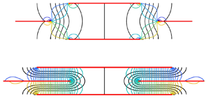
Figure 11 shows steady vertical flows at $Re_V = 0.001$ through different lattices. The plates are shown in red, and the flows repeat periodically in $x$ and $y$ with different periods, given in the figure caption. For the rectangular lattice, panels (a,b) exemplify two limiting regimes: $l_y/(l_x-1) \ll 1$ (the ratio is 1/2 in panel (a)) and $l_y/(l_x-1) \gg 1$ (the ratio is 20 in panel (b)). The rhombic lattice has three limiting regimes. One is the same as in panel (b), $l_y/(l_x-1) \gg 1$. Here the streamlines would be altered from those in panel (b) away from the gap between the plates, but would become the same near the gap. The second is $l_y/(l_x/2-1) \ll 1$ with $l_x > 2$ (e.g. panel (c) with $l_y/(l_x/2-1) = 1$ and $l_x = 2.5$) – here the vertical rows of plates do not overlap. The third is $l_y/(1-l_x/2) \ll 1$ with $l_x < 2$ (e.g. panel (d) with $l_y/(1-l_x/2) = 0.4$ and $l_x = 1.5$) – here the vertical rows of plates do overlap. Only panel (b) is firmly in the asymptotic regime, while the other panels are at moderate ratios. In all cases, the flows resemble the limiting flows, even at moderate ratios.

Figure 11.

Steady flows through plate lattices at $Re_V = 0.001$. Plates are red, streamlines are black and isopressure lines are blue, green and yellow (values in colour bars at right). (a) Flow through rectangular lattice with $l_x = 2$ and $l_y = 0.5$. (b) Flow through rectangular lattice with $l_x = 1.05$ and $l_y = 1$. (c) Flow through rhombic lattice with $l_x = 2.5$ and $l_y = 0.25$. (d) Flow through rhombic lattice with $l_x = 1.5$ and $l_y = 0.1$.

The steady versions of (2.2) and (2.3) are

(5.2)\begin{gather} \boldsymbol{u}\boldsymbol{\cdot}\boldsymbol{\nabla} \boldsymbol{u} ={-}\boldsymbol{\nabla} p +\frac{1}{{Re}_V} \nabla^2 \boldsymbol{u}, \end{gather}

(5.3)\begin{gather}\boldsymbol{\nabla} \boldsymbol{\cdot} \boldsymbol{u} = 0. \end{gather}

Integrating the $y$-component of (5.2) over a periodic unit cell, the left side vanishes because there is zero net vertical (or horizontal) outflow. So does the viscous term, because the inverse square root singularity in the shear stress diverges too slowly to produce a vertical resultant in the limit of zero plate thickness. Hence the integral of $-\partial _y p$ over the unit cell is zero. The integral has two contributions: one from the vertical change in $p$ across the unit cell, and the other from the jump in $p$ across the plate, resulting in a force applied by the plate to the fluid. Hence

(5.4)\begin{equation} 0 ={-}\int_{plate} [p]^+_- \, {\textrm{d} x} - l_x l_y \frac{{\rm \Delta} p_y}{l_y}, \end{equation}

where ${\rm \Delta} p_y$ is the change in pressure across the unit cell in the $y$ direction. For the rhombic lattice, with two plates in a double unit cell (figure 1(b)), the integral in (5.4) includes both plates and ${\rm \Delta} p_y$ is the change in pressure across the double unit cell in the $y$ direction. For steady flow with dimensionless mean $y$-velocity 1,

(5.5)\begin{equation} \langle P_{in} \rangle = P_{in} = \int_{plate} [p]^+_- \, {\textrm{d} x} ={-} l_x {\rm \Delta} p_y, \end{equation}

which relates the input power to the pressure difference across a unit cell in the $y$-direction. The latter can be determined analytically for the limiting cases of the flows in figure 11.

In the limit $l_y/(l_x-1) \ll 1$, the flow in panel (a) becomes Poiseuille flow in the $x$-interval between the plate edges (0 $\leq x \leq$ 1 in panel (a)), and zero flow in the rest of the flow field. Poiseuille flow is a good approximation to panel (a) even though $l_y/(l_x-1) = 1/2$, not very small. The lack of streamlines above and below the plates indicates slow flow there (the local density of streamlines is proportional to flow speed). In the interval 0 $\leq x \leq$ 1 the flow is nearly unidirectional with a parabolic profile for $v(x)$, and the isopressure contours are nearly equally spaced, corresponding to the constant pressure gradient of Poiseuille flow. Using Poiseuille flow to relate the pressure gradient ${\rm \Delta} p_y/l_y$ to the net fluid flux through the unit cell, $Q = 1 \cdot l_x$,

(5.6)\begin{equation} P_{in} ={-}l_x l_y \frac{{\rm \Delta} p_y}{l_y} = l_x l_y \frac{12 Q}{(l_x - 1)^3 {Re}_V} = \frac{12 l_x^2}{(l_x - 1)^2 {Re}_V} \frac{l_y}{l_x - 1}. \end{equation}

The last expression in (5.6) is written in terms of $l_y/(l_x-1)$, the parameter that sets the validity of the approximation.

The limit $l_y/(l_x-1) \gg 1$ is exemplified by figure 11(b). This is the Stokes flow through small gaps in a periodic array of plates. The black lines are again the streamlines. They show flow converging toward the gap, and a small recirculation region centred at the midpoints of the plates. To determine ${\rm \Delta} p_y$ and therefore $P_{in}$ in (5.5), we can use the Stokes-flow solution for a single gap in an infinite wall, derived by Hasimoto (Reference Hasimoto1958). In the region that is much farther from the gap than its width, the pressure is approximately constant, one constant above the wall and a different constant below the wall. In figure 11(b) this is shown by the coloured lines, isopressure contours (values at right). The solid line contours (dark blue and yellow) have pressures close to the values at distance 0.5 above and below the gap (i.e. far from the gap). The dashed lines (dark blue and yellow) have pressures 1 % above and below those of the solid lines. Hence, in panel (b) above and below the ‘cloverleaf’ regions near the gap bounded by the dashed lines, the pressure varies by less than 2 %. Therefore, the pressure field is essentially the same as that far from a single gap in an infinite wall. We approximate ${\rm \Delta} p_y$ in (5.5) as the difference between the far-field pressure constants for the infinite-wall case with net flux $Q$ through the gap, from Hasimoto (Reference Hasimoto1958): ${\rm \Delta} p_y/Q = -32 Re_V/(l_x-1)^2{\rm \pi}$ . Then we have

(5.7)\begin{equation} P_{in} ={-}l_x {\rm \Delta} p_y = \frac{32 l_x^2}{{\rm \pi} (l_x - 1)^2 {Re}_V}. \end{equation}

In figure 12 we plot $P_{in}$ for steady flows through rectangular lattices. Each row shows data for a different value of $Re_V$, up to 6.4, close to the threshold at which the steady flow state becomes unstable for some choices of $l_x$ close to 1. The first column shows $P_{in}$ versus $l_y$ for different choices of $l_x$ (coloured lines, values listed at right), at $U/V = 0$. The second column shows the same data in rescaled variables. $P_{in}$ is divided by $l_x^2/(l_x -1)^2 Re_V$, a factor that appears in both (5.6) and (5.7). On the horizontal axis, $l_y/(l_x-1)$ is used as the dependent variable. The black line shows the Poiseuille flow scaling (5.6), while the black cross shows the value 32/${\rm \pi}$ given by (5.7). The agreement is almost exact. The third and fourth columns show the same data for $U/V = 2$ and 8, respectively. Here, the Poiseuille flow result (5.6) can be modified by including a dimensionless cross-flow $U/V$ in the flow equations (Batchelor Reference Batchelor1967), resulting in a $v(x)$ that is linear plus exponential. In place of (5.6) we obtain

(5.8)\begin{equation} P_{in} = \frac{U}{V}l_x^2l_y\left[\frac{l_x-1}{{Re}_U} - \left(\frac{1}{2} +\frac{1}{\textrm{e}^{{Re}_U (l_x-1)} -1}\right)(l_x-1)^2\right]^{{-}1}, \end{equation}

with $Re_U = UL/\nu$. The value of $P_{in}$ in (5.8) tends to (5.6) as $Re_U \to 0$, i.e. if either $Re_V$ or $U/V$ $\to 0$, so the cross-flow has no effect in Stokes flow (as can also be seen by linearity). So only in the three panels near the lower right corner of figure 12 – i.e. the cases $(Re_V, U/V) = (0.8,8)$, (6.4, 2) and (6.4, 8) – do the coloured lines deviate noticeably from the black line; the deviation depends on $l_x$. The upper portions of the coloured lines are the data computed from steady Navier–Stokes solutions and the lower portions (separated by a gap from the upper portions) are the Poiseuille-plus-cross-flow approximations (5.8), different for each $l_x$, and which are linear in $l_y$. These line up almost exactly with the computed data. In summary, at small $Re_V$, $P_{in}$ grows linearly with $l_y/(l_x-1)$ when the ratio is small. The linear growth is because the rate of viscous energy dissipation per plate in the channel flows is proportional to the $y$-spacing between the plates, $l_y$. At large $l_y/(l_x-1)$, $P_{in}$ is independent of $l_y$ because the small-gap flow, and the corresponding rate of viscous energy dissipation, becomes independent of $l_y$.

Figure 12.

For steady flow through a rectangular lattice, $P_{in}$ versus $l_y$ (left column) and in rescaled variables (second through fourth columns) for different values of $Re_V$ (labelled at left) and $U/V$ (labelled at top).

We now consider analytical models for the rhombic lattice, with examples of flows in figure 11(c,d). The flow in panel (c) tends to two Poiseuille flows, each in a channel of width $l_x/2-1$, as $l_y/(l_x/2-1)$ becomes small. The flow in panel (d) tends to four Poiseuille flows, oriented horizontally, each in a channel of width $l_y$ and length $1-l_x/2$ (the horizontal overlap between the plates), as $l_y/(1-l_x/2)$ becomes small. The pressure drop between the ends of the channels is half the total pressure drop over the double unit cell. The special case $l_x = 2$ and $l_y \to 0$, at the boundary between these flows, is more complicated and we do not address it here. Using these approximations, we obtain for the limit $l_y/|l_x/2-1| \ll 1$,

(5.9)\begin{align} P_{in} = \left. \begin{cases} \displaystyle \frac{6 l_x^2}{(l_x/2 - 1)^2 {Re}_V} \frac{l_y}{l_x /2- 1}, & l_x > 2 \\ \displaystyle \frac{96 l_x^2}{(1-l_x/2)^2 {Re}_V} \left(\frac{1-l_x /2}{l_y}\right)^3, & l_x < 2 \end{cases} \right., \end{align}

using the appropriate expressions for ${\rm \Delta} p_y$. The case of large $l_y$ is essentially the same as figure 11(b), so for the double unit cell of the rhombic lattice, we have twice the $P_{in}$ of (5.7). We compare these results with the computed steady Navier–Stokes results in figure 13. We use only two values of $U/V$ now, 0 and 8, and the same $Re_V$ as in figure 12. The first column shows the unscaled data at $U= 0$. Unlike for the rectangular lattice, the scaling of $l_y$ changes from $l_y/|l_x/2-1|$ to $l_y/(l_x-1)$ at small and large $l_y$ respectively, so additional columns are needed to show the data with these separate scalings. The second and fourth columns show the small-$l_y$ scalings, with black lines showing the relationships in (5.9). In the bottom panel of the fourth column $((Re_V, U/V) = (6.4,8))$, the coloured lines with $l_x > 2$ are shifted at non-zero $Re_U$, due to the cross-flow effect discussed for the rectangular lattice (not rederived here). There is no visible shift for the $l_x < 2$ lines, because the effect of the cross-flow cancels for the four horizontal channel flows, two in each direction, in figure 11(d). The black crosses (third and fifth columns) again show the large $l_y/(l_x-1)$ values of $P_{in}$. The main difference from the rectangular lattice is the large growth in $P_{in}$ at small $l_y$ when $l_x < 2$. Propulsion occurs in many of these cases, e.g. at $l_y = 0.5$ and 0.7 (top and middle rows of figure 14, Part 2). However, the peak Froude efficiency decreases noticeably when $l_x$ drops below 2 and when $l_y$ decreases in most of these cases.

Figure 13.

For steady flow through a rhombic lattice, $P_{in}$ versus $l_y$ (left column) and in rescaled variables (second through fifth columns) for different values of $Re_V$ (labelled at left) and $U/V$ (labelled at top).

5.1. Input power for flows through flapping lattices

Now we consider the input power in the unsteady, fully nonlinear flapping problem, at $Re = 10$–$70$. This is the range of $Re$ that we investigate for propulsion in Part 2, because it corresponds to periodic lattice flows, for which we can compute long time averages accurately. For the steady problem, the flows were plotted at much lower Reynolds number ($Re_V = 0.001$) in figure 11, mainly because an analytical solution is available in this limit for panel (b), the small-gap case. However, the Poiseuille flows with a cross-flow or without (as in panels (a,c) and (d) remain valid at larger $Re_V$, until they become unstable (at $Re_V = O(10^3)$ (Schmid, Henningson & Jankowski Reference Schmid, Henningson and Jankowski2002), above the Reynolds numbers in the present study). Non-dimensionalizing (5.6) using $\nu /L$ in place of $V$, consistent with the unsteady $\langle {\tilde P}_{in}\rangle$ results in this paper, we have

(5.10)\begin{equation} {\tilde P}_{in} = \frac{12 l_x^2}{(l_x - 1)^2}{Re}_V^2 \frac{l_y}{l_x - 1}. \end{equation}

The small-gap flow in figure 11(b) changes to a jet flow (e.g. figure 3 of Part 2) as the Reynolds number rises to 20. For $Re = 10$–$70$ the flow is intermediate between viscous dominated (resulting in (5.7)) and inertia dominated. In the latter case, the momentum theorem can be used to calculate ${\tilde P}_{in}$ in the case of steady inertia-dominated (high-$Re$) flow. The calculation is the same as for the steady drag on an infinite, periodically perforated plate, given in Batchelor (Reference Batchelor1967, § 5.15). In the small-gap limit $l_y/(l_x - 1) \gg 1$, the pressure drop through a unit cell of our periodic lattice becomes the same as that through the periodically perforated plate, which in our notation (and non-dimensionalized by $\rho _f V^2$) is

(5.11)\begin{equation} {\rm \Delta} p_y ={-}\frac{1}{2(l_x-1)^2}. \end{equation}

The pressure is assumed to follow Bernoulli's law on the upstream sides of the plates, while on the downstream sides, where separated flow occurs, it is assumed constant and equal to that in the gap (see Batchelor (Reference Batchelor1967) for details). The input power follows from (5.5)

(5.12a,b)\begin{equation} P_{in} = \frac{l_x}{2(l_x-1)^2};\quad {\tilde P}_{in} = \frac{l_x}{2(l_x-1)^2}{Re}_V^3. \end{equation}

where again, ${\tilde P}_{in}$ has been non-dimensionalized using $\nu /L$ in place of $V$, consistent with the unsteady results in this paper. For both Stokes flow (5.7) and separated flow (5.12a,b) with small $l_x -1$, $P_{in}$ diverges like $(l_x -1)^{-2}$, though with different prefactors.

Time-averaged input power for the rectangular lattice is plotted in figure 14 at two values of $Re$ and $A/L$ (labelled at left) and $U/fA$ (labelled at top) in the ranges already considered. The unscaled $\langle {\tilde P}_{in} \rangle$ data are shown in the first column. $\langle {\tilde P}_{in} \rangle$ is rescaled according to the small-$l_y$ Poiseuille flow scaling (5.10) in the second and fourth columns, and according to the large-$l_y$ separated flow scaling (5.12a,b) in the third and fifth columns, with $Re$ (from (2.5a–d)) in place of $Re_V$. The error bars show the range of values within one standard deviation of $\langle {\tilde P}_{in} \rangle$, computed using the last five period averages of ${\tilde P}_{in}(t)$. In many cases (i.e. $Re = 10$, small $l_y$), ${\tilde P}_{in}(t)$ is periodic, so the error bar has almost zero height, and the upper and lower horizontal hash marks overlap, appearing as a single hash mark. At $Re = 70$ and larger $l_y$, the vertical extent of the error bar is noticeable, and gives a measure of the non-periodicity of the data.

Figure 14.

Time-averaged input power $\langle {\tilde P}_{in} \rangle$ for flapping rectangular lattices at $U/fA = 1$ (first to third columns) and 4 (fourth and fifth columns), at $Re = 10$ and 70 and $A/L = 0.2$ and 0.8 (values labelled at left), for various $l_x$ (listed separately for each $Re$ at right). The error bars show the range of values within one standard deviation of $\langle {\tilde P}_{in} \rangle$. The standard deviation is computed using the last five period averages of ${\tilde P}_{in}(t)$.

Although the data are more scattered in the unsteady case, they are qualitatively similar to the steady case (figure 12), including the shift at increasing $l_x$ in the Poiseuille flow (linear growth regime). The steady problem neglected the effects of unsteadiness (an oscillating instead of steady vertical flow) and nonlinearity in the Navier–Stokes equations. We extended the steady model to the case of an unsteady but linearized model,

(5.13)\begin{equation} \partial_t v + U\partial_x v ={-}P_y \ \textrm{e}^{2{\rm \pi} i t} +\frac{1}{{Re}_f} \partial_{xx} v, \end{equation}

for a harmonically oscillating channel flow $v(x,t) = V_0(x)\textrm {e}^{2{\rm \pi} i t}$ with cross-flow. Analytical solutions are again possible, but more complicated than the steady case because we are back in the five-dimensional parameter space. We did not analyse the results in detail but they seemed to agree qualitatively with the small $l_y$-results in figures 12 and 14. Despite the complications due to vortex shedding and non-periodicity, the steady models and the fully nonlinear simulations agree qualitatively in the behaviour of $\langle {\tilde P}_{in} \rangle$ – linear growth at small $l_y/(l_x-1)$ in the second and fourth columns of figure 14, saturation at large $l_y/(l_x-1)$ in the third and fifth columns. The main discrepancy is that the $Re = 10$ data have a larger magnitude than the $Re = 70$ data. A better fit is provided by the relation $\langle {\tilde P}_{in} \rangle \sim {Re}^3$ (typical for pressure losses at high $Re$, as in the third and fifth columns), rather than the $\sim {Re}^2$ scaling for steady Poiseuille flow used in the second and fourth columns of figure 14.

The fully nonlinear $\langle {\tilde P}_{in} \rangle$ data for the rhombic lattices are presented in figure 15. As for the rectangular lattices, the data are presented with different scalings at small $l_y$ (second and fourth columns) and large $l_y$ (third and fifth columns). In spite of the effects of non-periodicity, there is good qualitative agreement between the unsteady and steady (figure 13) cases. In the second and fourth columns, there is a clear divergence at small $l_y/|l_x/2-1|$ between the lines with $l_x >2$ (red and orange) and the remaining lines. We did not compute cases at $l_y/|l_x/2-1|$ as small as in figure 13, however, because they are not useful for locomotion, and in the unsteady case, the parameter space is larger and each simulation requires much more computing time. Again, the $Re = 10$ data are generally larger than the $Re = 70$ data in the second and fourth columns, perhaps indicating the importance of pressure losses beyond those of Poiseuille flow at higher $Re$. In the third and fifth columns, the lines at various $l_x$ seem to agree reasonably well at large $l_y/(l_x-1)$.

Figure 15.

Time-averaged input power $\langle {\tilde P}_{in} \rangle$ for flapping rhombic lattices at $U/fA = 1$ (first to third columns) and 4 (fourth and fifth columns), at $Re = 10$ and 70 and $A/L = 0.2$ and 0.8 (values labelled at left), for various $l_x$ (listed separately for each $Re$ at right). The error bars show the range of values within one standard deviation of $\langle {\tilde P}_{in} \rangle$. The standard deviation is computed using the last five period averages of ${\tilde P}_{in}(t)$.

6. Summary and conclusions

We have introduced a computational model for the collective locomotion of lattices of flapping plates. In our simulations, we used a rectilinear grid with grid points concentrated near the singularities at the plates’ edges. The condition number of the discrete Laplacian remains many orders of magnitude below 10$^{16}$ for the grids used in this paper, so round-off error is not a major obstacle. For a Laplace equation with similar singular behaviour, we found that the method gives better than 1 % accuracy in the solution and the integral of its gradient along the plate for modest mesh sizes, and converges as grid spacing to the 3/2 power.

We first used the method to determine the propulsive properties of an isolated flapping plate in this specific context (a plate with zero thickness flapping in a flows with different upstream velocities). The solutions show many properties that resemble those of previous flapping-foil studies: a reversed von Kármán street at certain oncoming flow speeds, more complicated vorticity fields at lower speeds and a single stable self-propelled speed. The Strouhal numbers for maximal Froude efficiency increase from approximately 0.4 to $\gg$1 as $Re_f$ decreases from 200 to 10, while the Strouhal numbers corresponding to the self-propelled speeds increase from 0.25 to $\gg$1 in the same range of $Re_f$. The maximum Froude efficiency for an isolated plate decreases from 0.06 at $Re_f = 200$ to less than 0.003 at $Re_f = 10$. These values are much lower than for higher-$Re$ swimming fish and robots. This is consistent with the fact that flapping locomotion is not possible when $Re$ decreases below a critical value of order unity, and there the maximum Froude efficiency becomes zero. The Pareto-optimal flapping amplitudes for maximizing speed at a given mean input power stay nearly fixed at 0.2–0.3. By contrast, the optimal flapping frequency increases with increasing self-propelled speed and/or input power. The input power scales as flapping amplitude and frequency, both raised to the third power, and depends only weakly on the oncoming flow velocity.

We then studied the input power required for flapping lattices of plates, before studying their propulsive efficiencies in Part 2 (Alben Reference Alben2021). The input power was estimated theoretically using steady flow models, which predict different scaling laws depending on the values of $l_x$ and $l_y$ for each lattice type.

For rectangular lattices, when the transverse spacing $l_y$ is much smaller than the tandem spacing (i.e. $l_y \ll l_x-1$), the flow between the plates is approximately Poiseuille flow, and is proportional to the transverse spacing and inversely proportional to the cube of the tandem spacing. By contrast, if the tandem spacing is small relative to the plate length and to the transverse spacing ($l_x-1 \ll 1, l_y$), we have small gap flow with input power inversely proportional to the square of the tandem spacing. Superposing a tangential flow with the transverse flows, the input power increases in proportion to the product of the tangential flow speed and the tandem spacing.

The input power for a rhombic lattice can also be approximated by Poiseuille flows and small-gap flows in the same limits. The main difference with rectangular lattices is that input power is much larger when the transverse spacing is small ($l_y \ll l_x-1$) and neighbouring rows of plates overlap ($l_x < 2$), so flow is forced through the small gaps between the plates.

The lattice flows studied in Part 2 occur at intermediate $Re$, between 10 and 70. The Poiseuille flow models remain valid in this regime, but the small-gap flows need to be modified. In the steady case, they can be modelled as separated flows through periodically perforated plates, with input power calculated by an integrated momentum balance. The input power is again inversely proportional to the square of the tandem spacing, but with a different prefactor than at small $Re$.

Compared to the steady flow models, the unsteady flows through lattices showed qualitatively similar input power trends at $Re = 10$ and 70 and two different flapping amplitudes, across ranges of $l_x$ and $l_y$ that we probe further in Part 2. The power grows approximately linearly in $l_y$ when $l_y \ll l_x-1$, and then saturates as $l_y$ becomes comparable to or larger than $l_x-1$. There is increased irregularity in the $Re = 70$ data due to non-periodicity of many of these flows for $l_y > 1$.

In Part 2 we discuss various examples of lattice flows in the $Re$ range 10–70, the corresponding thrust and drag forces on the plates, measures of propulsive efficiency, and self-propelled states.