1 Introduction
Parametrically forced stratified flows are of both fundamental and practical interest, with many open questions remaining to be addressed, particularly in regards to resonances and internal wave breaking for continuously stratified flows (Yih Reference Yih1960; Thorpe Reference Thorpe1968; McEwan Reference McEwan1971; McEwan, Mander & Smith Reference McEwan, Mander and Smith1972; Orlanski Reference Orlanski1972, Reference Orlanski1973; McEwan & Robinson Reference McEwan and Robinson1975; Drazin Reference Drazin1977; Sherman, Imberger & Corcos Reference Sherman, Imberger and Corcos1978; McEwan Reference McEwan1983; Thorpe Reference Thorpe1994; Bouruet-Aubertot, Sommeria & Staquet Reference Bouruet-Aubertot, Sommeria and Staquet1995; Benielli & Sommeria Reference Benielli and Sommeria1998; Staquet Reference Staquet2004; Dauxois et al. Reference Dauxois, Joubaud, Odier and Venaille2018). Even the onset of instability has not been clearly resolved. This is in sharp contrast to the case of parametrically forced interfacial flows, such as the Faraday wave problem (Miles & Henderson Reference Miles and Henderson1990). In the inviscid idealization of the Faraday problem, the onset of instability is well characterized by independent Mathieu equations for each instability mode as the modes are orthogonal (Benjamin & Ursell Reference Benjamin and Ursell1954). When viscous stress at the interface is taken into account, even though the modes are no longer orthogonal and their damping depends on their wavenumber, the corresponding Floquet analysis (Kumar & Tuckerman Reference Kumar and Tuckerman1994) gives very good agreement with experiments (Fauve et al. Reference Fauve, Kumar, Laroche, Beysens and Garrabos1992) for the onset of instability.
Yih (Reference Yih1960) considered the linear stability of a continuously stratified and laterally unbounded inviscid fluid subjected to vertical vibration. The resultant inviscid Mathieu equations for the instability modes were essentially the same as those of Benjamin & Ursell (Reference Benjamin and Ursell1954). Motivated by the question of internal wave breaking, Thorpe (Reference Thorpe1968) built on Yih’s work by analytically determining the eigenmodes for a laterally confined stratified system, and set up an experiment with plungers in the two opposing side walls to perturb a continuously stratified brine solution. The two-dimensional standing internal wave modes were analytically determined to third order in wave amplitude for an inviscid, diffusionless, stably and linearly stratified fluid confined in a rectangular container (Thorpe Reference Thorpe1968). Thorpe observed a number of resonantly driven modes near the frequencies predicted by the linear inviscid theory, and qualitatively described wave breaking and mixing for large-amplitude forcing. However, he was only able to observe modes of a specific parity and was unable to quantitatively study the large-amplitude responses. Also, his experiment suffered from the presence of internal wave beams emanating from the junctions where the side walls and plungers met, which interacted with the driven modes. Also motivated by two-dimensional internal wave breaking and transition to turbulence, and whether triadic resonances are involved, McEwan (Reference McEwan1971) devised an experiment similar to that of Thorpe (Reference Thorpe1968), but using paddles instead of plungers. Those experiments also generated internal wave beams at the junctions of the paddles and the container.
Benielli & Sommeria (Reference Benielli and Sommeria1998) also studied linearly stratified flow in a rectangular container, but in contrast to the earlier experiments, they used vertical oscillations to perturb the flow. This had the advantage of not having any differential motion of the container walls, thus avoiding the production of wave beams. They were able to describe the primary and secondary instabilities, observing the fundamental eigenmode and its apparent harmonics lose stability to wave breaking. They considered a small forcing frequency interval covering the resonance interval for the lowest-order spatial mode. Although they were unable to experimentally determine the forcing frequency bounds for the resonance tongue, they did observe intermittent bursting and wave breaking.
In this paper, we study the nonlinear dynamics via numerical simulations of the two-dimensional Navier–Stokes equations using the Boussinesq approximation. The restriction to two-dimensional flow is motivated by the experimental results of Benielli & Sommeria (Reference Benielli and Sommeria1998) which showed that the flow remained two-dimensional in their short spanwise aspect ratio container, unless the forcing amplitude was large enough to cause wave breaking. McEwan (Reference McEwan1983) also noted in his experiments in a similar rectangular container, but with the flow driven by a paddle, that the flow was predominantly two-dimensional, although small patches of fine-scale three-dimensional distortions occurred intermittently due to localized instabilities.
We begin by examining the onset of instability over a wide range of forcing frequencies, from nearly zero to a little over two and a half times the buoyancy frequency. The loci of lowest forcing amplitude for a non-static response flow as a function of forcing frequency broadly agrees well with the Floquet analysis of Yalim, Lopez & Welfert (Reference Yalim, Lopez and Welfert2018) that used temperature stratification. While Floquet analysis determines the amplitudes and frequencies at which the basic state loses stability, it provides no information about the nonlinear dynamics that results as perturbations grow to finite amplitudes. The nonlinear results presented here show that many of the resonance tongues have a hysteretic region on their low-frequency side. Also, complex dynamics is often observed at or very near onset. These two effects contribute to the problems identifying the edges of the resonance tongues experimentally (Benielli & Sommeria Reference Benielli and Sommeria1998). For the lowest-order spatial mode, we then examine in detail the dynamics near the tip of its resonance tongue, reconciling the complex dynamics observed in our nonlinear simulations with what is expected from a dynamical systems perspective near onset.
2 Governing equations and numerics
Consider a fluid of kinematic viscosity
 $\unicode[STIX]{x1D708}$
, thermal diffusivity
 $\unicode[STIX]{x1D705}$
and coefficient of volume expansion
 $\unicode[STIX]{x1D6FD}$
contained in a square cavity of side lengths
 $L$
. The cavity side walls are thermally insulated (adiabatic) while the end walls are held at constant temperatures. The temperature difference between the top and bottom walls is
 $\unicode[STIX]{x0394}T=T_{T}-T_{B}>0$
. Gravity
 $g$
acts downwards in the negative
 $z$
direction. In the absence of any other external force, the fluid is linearly stratified. The cavity is subjected to harmonic oscillations in the vertical direction with angular frequency
 $\unicode[STIX]{x1D6FA}$
and amplitude
 $\ell$
. The non-dimensional temperature is
 $T=(T^{\ast }-T_{B})/\unicode[STIX]{x0394}T-0.5$
. The length scale
 $L$
and time scale
 $1/N$
are used to non-dimensionalize, where
 $N=\sqrt{g\unicode[STIX]{x1D6FD}\unicode[STIX]{x0394}T/L}$
is the buoyancy frequency. A Cartesian coordinate system
 $\boldsymbol{x}=(x,z)\in [\pm 0.5,\pm 0.5]$
is fixed with its origin at the centre of the cavity, and the corresponding velocity is
 $\boldsymbol{u}=(u,w)$
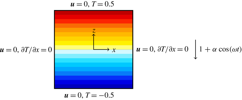
. Figure 1 is a schematic of the set-up. Under the Boussinesq approximation, the non-dimensional governing equations in the frame of reference fixed to the oscillating cavity (the cavity frame) are
 $$\begin{eqnarray}\left.\begin{array}{@{}c@{}}\displaystyle \frac{\unicode[STIX]{x2202}\boldsymbol{u}}{\unicode[STIX]{x2202}t}+\boldsymbol{u}\boldsymbol{\cdot }\unicode[STIX]{x1D735}\boldsymbol{u}=-\unicode[STIX]{x1D735}p+\frac{1}{R_{N}}\unicode[STIX]{x1D6FB}^{2}\boldsymbol{u}+(1+\unicode[STIX]{x1D6FC}\cos \unicode[STIX]{x1D714}t)T\boldsymbol{e}_{z},\quad \unicode[STIX]{x1D735}\boldsymbol{\cdot }\boldsymbol{u}=0,\\ \displaystyle \frac{\unicode[STIX]{x2202}T}{\unicode[STIX]{x2202}t}+\boldsymbol{u}\boldsymbol{\cdot }\unicode[STIX]{x1D735}T=\frac{1}{\unicode[STIX]{x1D70E}R_{N}}\unicode[STIX]{x1D6FB}^{2}T,\end{array}\right\}\end{eqnarray}$$
where
 $p$
is the reduced pressure. The system is governed by four non-dimensional parameters,
 $$\begin{eqnarray}\left.\begin{array}{@{}ll@{}}\text{buoyancy number} & R_{N}=NL^{2}/\unicode[STIX]{x1D708},\\ \text{Prandtl number} & \unicode[STIX]{x1D70E}=\unicode[STIX]{x1D708}/\unicode[STIX]{x1D705},\\ \text{forcing frequency} & \unicode[STIX]{x1D714}=\unicode[STIX]{x1D6FA}/N,\\ \text{forcing amplitude} & \unicode[STIX]{x1D6FC}=\unicode[STIX]{x1D6FA}^{2}\ell /g.\end{array}\right\}\end{eqnarray}$$
In this study,
 $R_{N}=2\times 10^{4}$
and
 $\unicode[STIX]{x1D70E}=1$
are fixed, and we consider
 $0<\unicode[STIX]{x1D714}\leqslant 2.5$
and
 $0<\unicode[STIX]{x1D6FC}\leqslant 1$
.
Schematic showing the initial isotherms, the boundary conditions, coordinate system and body force (harmonic gravity modulation).

The velocity boundary conditions are no slip, and in the cavity frame these are
 $u=w=0$
on all four boundaries. The top and bottom end wall temperature boundary conditions are
 $T|_{z=\pm 0.5}=\pm 0.5$
and on the side walls
 $\unicode[STIX]{x2202}_{x}T|_{x=\pm 0.5}=0$
. The experimental studies (e.g. Thorpe Reference Thorpe1968; McEwan Reference McEwan1971, Reference McEwan1983; Benielli & Sommeria Reference Benielli and Sommeria1998) used salt stratification, which has a very slow diffusivity (the ratio of kinematic viscosity to salt diffusivity, the Schmidt number, is of order 700). The boundary condition for salt at a solid wall is zero flux, so that a constant linear stratification fails in a thin boundary layer (whose thickness grows slowly with time) on the bottom wall (and at the top wall if it is rigid; some experiments used a free surface). The zero flux condition means that eventually, the system becomes homogeneous. Of course, the time scale for homogenization is very slow compared to the dynamic time scales of interest in the experiments, but for a theoretical analysis both of these effects become problematic. The use of heat rather than salt stratification, with fixed temperatures on the top and bottom walls and insulating (zero flux) side wall boundary conditions leads to linear temperature stratification as an equilibrium solution for the temperature equation. This, together with no-slip boundary conditions for the velocity, gives a basic state which is linearly stratified and static in the frame of reference of the vertically oscillating container, whose linear stability has been studied using Floquet analysis (Yalim et al.
Reference Yalim, Lopez and Welfert2018). When the viscous time scale is large compared to the buoyancy time scale, the viscous Floquet modes resemble the inviscid eigenmodes of the unforced problem (Thorpe Reference Thorpe1968), except for the presence of thin boundary layers.
Space is discretized via spectral collocation with Chebyshev polynomials of degree
 $M$
in barycentric form, and time evolution uses the fractional-step improved projection scheme of Mercader, Batiste & Alonso (Reference Mercader, Batiste and Alonso2010). We have used this method previously with related problems in Cartesian coordinates (Lopez et al.
Reference Lopez, Welfert, Wu and Yalim2017; Wu, Welfert & Lopez Reference Wu, Welfert and Lopez2018). Most of the results presented in this study were obtained with Chebyshev polynomials of degree
 $M=72$
in both the
 $x$
and
 $z$
directions. For
 $\unicode[STIX]{x1D714}>0.30$
, the forcing period was discretized into 1000 time steps. For
 $\unicode[STIX]{x1D714}\leqslant 0.30$
, up to 5000 time steps per period were used.
The kinetic energy
 $E_{K}$
and the normalized thermal
 ${\mathcal{L}}^{2}$
measure
 $E_{T}$
are used to monitor the flows,
 $$\begin{eqnarray}E_{K}=\frac{1}{2}\int _{-0.5}^{0.5}\int _{-0.5}^{0.5}(u^{2}+w^{2})\,\text{d}x\,\text{d}z\quad \text{and}\quad E_{T}=12\int _{-0.5}^{0.5}\int _{-0.5}^{0.5}T^{2}\,\text{d}x\,\text{d}z;\end{eqnarray}$$
 $E_{T}$
is normalized by the thermal
 ${\mathcal{L}}^{2}$
measure of the basic state
 $\int _{-0.5}^{0.5}\int _{-0.5}^{0.5}z^{2}\,\text{d}x\,\text{d}z=1/12$
.
To characterize the amplitude of the flow’s response, we compute the temporal standard deviation of the kinetic energy
 $\unicode[STIX]{x1D6F4}_{K}$
and the temporal variance of the horizontal velocity
 $\unicode[STIX]{x1D6F4}_{u}^{2}$
at the point
 $\boldsymbol{x}_{p}=(x_{p},z_{p})=(1/\sqrt{8},1/\sqrt{8})$
.
3 Symmetries
The governing equations are equivariant to a group symmetry
 ${\mathcal{G}}$
generated by reflections in
 $x$
and in
 $z$
. The actions of these reflections are
 $$\begin{eqnarray}\displaystyle & \displaystyle {\mathcal{K}}_{x}(u,w,T)(x,z,t)=(-u,w,T)(-x,z,t), & \displaystyle\end{eqnarray}$$
 $$\begin{eqnarray}\displaystyle & \displaystyle {\mathcal{K}}_{z}(u,w,T)(x,z,t)=(u,-w,-T)(x,-z,t). & \displaystyle\end{eqnarray}$$
The symmetry group
 ${\mathcal{G}}$
has four elements,
 ${\mathcal{G}}=\{{\mathcal{I}},{\mathcal{K}}_{x},{\mathcal{K}}_{z},{\mathcal{R}}_{\unicode[STIX]{x03C0}}\}$
, where
 ${\mathcal{I}}$
is the identity and
 ${\mathcal{R}}_{\unicode[STIX]{x03C0}}={\mathcal{K}}_{x}\circ {\mathcal{K}}_{z}={\mathcal{K}}_{z}\circ {\mathcal{K}}_{x}$
is a
 $\unicode[STIX]{x03C0}$
-rotation;
 ${\mathcal{G}}$
is a
 $Z_{2}\times Z_{2}$
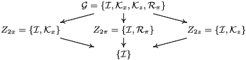
group. The lattice of subgroups of
 ${\mathcal{G}}$
is presented in table 1.
Hasse diagram of the lattice of subgroups of the group
 ${\mathcal{G}}=\{{\mathcal{I}},{\mathcal{K}}_{x},{\mathcal{K}}_{z},{\mathcal{R}}_{\unicode[STIX]{x03C0}}\}$
.

The basic state B is
 $$\begin{eqnarray}\boldsymbol{u}=0,\quad T=z,\quad \text{and}\quad p=0.5z^{2}(1+\unicode[STIX]{x1D6FC}\cos \unicode[STIX]{x1D714}t),\end{eqnarray}$$
in the cavity frame. It is
 ${\mathcal{G}}$
invariant. The system, being periodically forced, is invariant to a time translation
 $$\begin{eqnarray}{\mathcal{P}}_{\unicode[STIX]{x1D70F}}(u,w,T)(x,z,t)=(u,w,T)(x,z,t+\unicode[STIX]{x1D70F}),\end{eqnarray}$$
where
 $\unicode[STIX]{x1D70F}=2\unicode[STIX]{x03C0}/\unicode[STIX]{x1D714}$
is the forcing period. As parameters are varied, instabilities lead to other solutions appearing, which may have broken symmetries. Time dependent states evolve on temporally invariant manifolds. For example, limit cycles have a one-dimensional manifold and 2-tori have a two-dimensional manifold. These states may be pointwise invariant with respect to a spatial symmetry, i.e. at any point in time, the state is invariant to the said symmetry. When
 ${\mathcal{G}}$
invariance is broken, the bifurcating state is pointwise invariant to only one of the generators of
 ${\mathcal{G}}$
. The states may be only setwise invariant, whereby applying the symmetry to the state transforms it onto the same invariant manifold. If the setwise symmetry of a state is broken, applying the symmetry results in another state on a different manifold that is the symmetric image of the original manifold. Also, for any state
 ${\mathcal{S}}$
that is not synchronous with the forcing, there is a conjugate state
 ${\mathcal{P}}_{\unicode[STIX]{x1D70F}}({\mathcal{S}})$
.
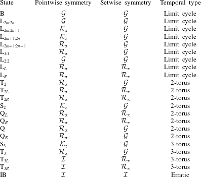
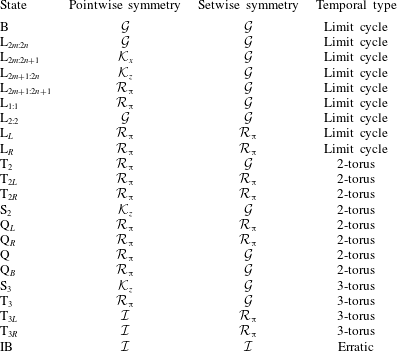
Table 2 is a list of the states that we report on in this study, together with their pointwise and setwise invariances.
List of states observed and their symmetries. B: basic state; L: limit cycles; T
 $_{2}$
, Q and S
 $_{2}$
: 2-tori; T
 $_{3}$
and S
 $_{3}$
: 3-tori; IB: an intermittently bursting state.
4 Primary instabilities
We begin with a broad overview of the flow response for
 $R_{N}=2\times 10^{4}$
and
 $\unicode[STIX]{x1D70E}=1$
over a large range of forcing frequencies and amplitudes,
 $\unicode[STIX]{x1D714}\in (0,2.5)$
and
 $\unicode[STIX]{x1D6FC}\in (0,1]$
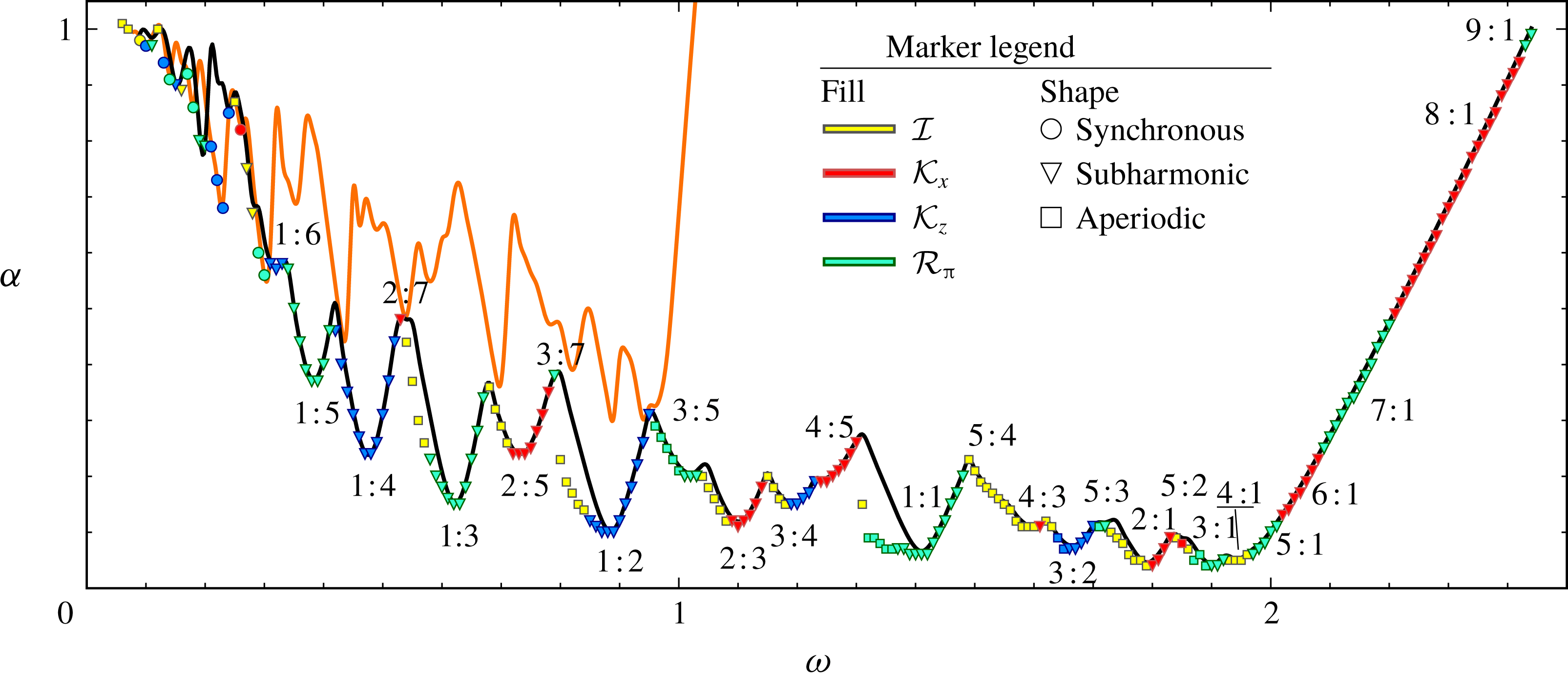
. This is summarized in figure 2, where the two solid curves are the loci in
 $(\unicode[STIX]{x1D714},\unicode[STIX]{x1D6FC})$
where the Floquet analysis of the basic state (Yalim et al.
Reference Yalim, Lopez and Welfert2018) indicates that a single multiplier leaves the unit circle either through
 $+1$
(synchronous; orange curve) or through
 $-1$
(subharmonic; black curve). Below both curves, all Floquet multipliers have modulus less than one (they are all inside the unit circle) and the basic state is stable. The spatial structures of the Floquet modes are very similar to those of the corresponding inviscid eigenmodes of the unforced cavity (Thorpe Reference Thorpe1968), which consist of
 $m$
cells in the horizontal and
 $n$
cells in the vertical directions. Regardless of whether the forced flow is synchronous or subharmonic, its frequency (the response frequency
 $\unicode[STIX]{x1D714}_{R}$
) is always very close to the eigenfrequency of the corresponding unforced inviscid eigenmode. For synchronous flow
 $\unicode[STIX]{x1D714}_{R}=\unicode[STIX]{x1D714}$
and for subharmonic flow
 $\unicode[STIX]{x1D714}_{R}=\unicode[STIX]{x1D714}/2$
. The forced viscous modes differ from the inviscid eigenmodes primarily due to the presence of viscous boundary layers. The details of these boundary layers are given in Yalim et al. (Reference Yalim, Lopez and Welfert2018). Superimposed on the Floquet stability boundaries in figure 2 are symbols indicating the lowest
 $\unicode[STIX]{x1D6FC}$
for each considered frequency
 $\unicode[STIX]{x1D714}$
that a non-trivial state was found. The colour and shape of the symbols indicate the symmetry (or lack thereof) of the state and whether it is synchronous or subharmonic with respect to the forcing frequency. Synchronous states are only observed for low frequencies,
 $\unicode[STIX]{x1D714}\lesssim 0.3$
, and these are irregularly interspersed with subharmonic states. The figure shows a complicated nesting of resonances tongues, each tongue corresponding to a resonant excitation of an
 $m:n$
viscous eigenmode. The observed tongues correspond to low values of
 $m$
and
 $n$
(typically less than 10), and the finite Farey sequence of
 $m+p:n+q$
intermediate tongues nested between
 $m:n$
and
 $p:q$
tongues is consistent with the results of the Floquet analysis. More locally, the agreement between the Floquet stability results and the nonlinear simulations is also very good, particularly on the high-
 $\unicode[STIX]{x1D714}$
side of a resonance tongue, indicating that the primary instability is supercritical there. On the low-
 $\unicode[STIX]{x1D714}$
side, there are considerable discrepancies between the two, particularly for the resonance tongues
 $1:n$
with
 $n=1$
, 2, and 3. This is due to the instability being subcritical with the region of hysteresis being larger for smaller
 $n$
. When nonlinear simulations use the basic state as the initial condition for increasing
 $\unicode[STIX]{x1D6FC}$
at fixed
 $\unicode[STIX]{x1D714}$
, the first non-trivial result agrees very well with the Floquet analysis. The gaps between the nonlinear simulation symbols shown in the figure and the Floquet curve indicate the extent of the hysteresis regions where both the basic state and non-trivial solutions are attracting.
Stability boundaries in forcing frequency
 $\unicode[STIX]{x1D714}$
and forcing amplitude
 $\unicode[STIX]{x1D6FC}$
space illustrating internal wave resonance tongues. The black curve is the boundary for subharmonic instability and the orange curve is the boundary for synchronous instability, both determined via Floquet analysis (Yalim et al.
Reference Yalim, Lopez and Welfert2018). The symbols are placed at the lowest
 $\unicode[STIX]{x1D6FC}$
for a given
 $\unicode[STIX]{x1D714}$
at which a non-trivial state is found via nonlinear simulations; the colour and shape of the symbols correspond to their pointwise symmetry and temporal response, as indicated. Also indicated are the
 $m:n$
spatial structure of the nonlinear states.

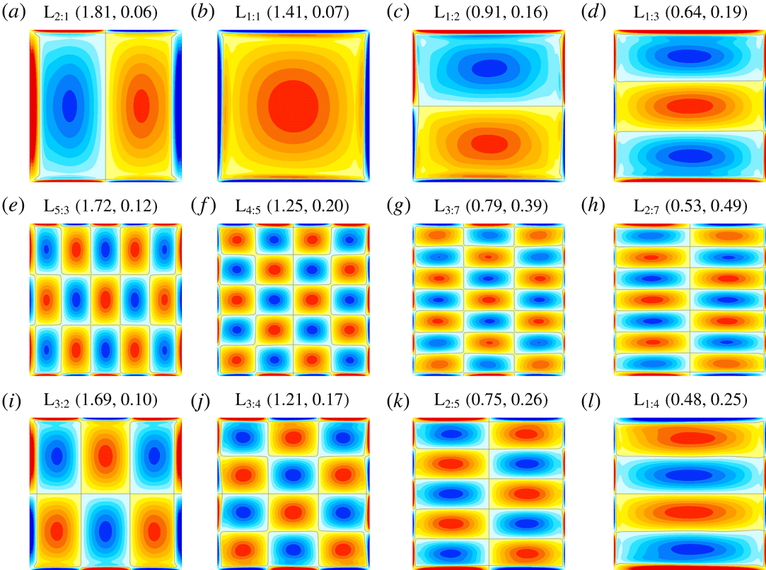
Vorticity at phase
 $\unicode[STIX]{x03C0}/2$
in the forcing for some of the subharmonic limit cycles L
 $_{m:n}$
at
 $(\unicode[STIX]{x1D714},\unicode[STIX]{x1D6FC})$
as indicated. See supplementary movie 1 for animations of L
 $_{1:1}$
, L
 $_{1:2}$
and L
 $_{2:1}$
over one response period (two forcing periods).

Time-averaged vorticity for the subharmonic limit cycle responses at
 $(\unicode[STIX]{x1D714},\unicode[STIX]{x1D6FC})$
as indicated, corresponding to the states in figure 3.

Figure 3 shows snapshots of the subharmonic limit cycles L
 $_{m:n}$
near the tips of the leading tongues, obtained from the nonlinear simulations at the same forcing amplitudes and frequencies,
 $\unicode[STIX]{x1D6FC}$
and
 $\unicode[STIX]{x1D714}$
, as was used in the Floquet analysis to illustrate the structure of the corresponding viscous modes V
 $_{m:n}$
shown in figure 3 of Yalim et al. (Reference Yalim, Lopez and Welfert2018). The structures are very similar, but do show subtle differences due to nonlinear harmonics in L
 $_{m:n}$
. Linearizing the Navier–Stokes equations about the basic state (3.3) introduces additional symmetries that the nonlinear system is not invariant to. Another distinction between the nonlinear states L
 $_{m:n}$
and the corresponding Floquet modes V
 $_{m:n}$
is that whereas V
 $_{m:n}$
have a time-invariant spatial structure that is harmonically modulated in time, this is not the case for L
 $_{m:n}$
. Supplementary movie 1 available at https://doi.org/10.1017/jfm.2019.347 shows animations of L
 $_{1:1}$
, L
 $_{1:2}$
, and L
 $_{2:1}$
over one response period (i.e. two forcing periods), from which it is evident that there is a propagation from the top and bottom end wall boundary layers into the interior accompanied with a propagation from the interior to the side wall boundary layers. This is more pronounced for larger
 $m$
and
 $n$
(movies are not shown). This nonlinearity results in a non-zero mean flow. Figure 4 shows the vorticity of the mean flow of the L
 $_{m:n}$
in figure 3; they all have the spatial structure of the corresponding first harmonic, i.e. the mean flow for L
 $_{m:n}$
has
 $2m:2n$
spatial structure.
5 The tip of the
 $\mathbf{1}\boldsymbol{ : }\mathbf{1}$
resonance tongue

We now focus on the
 $1:1$
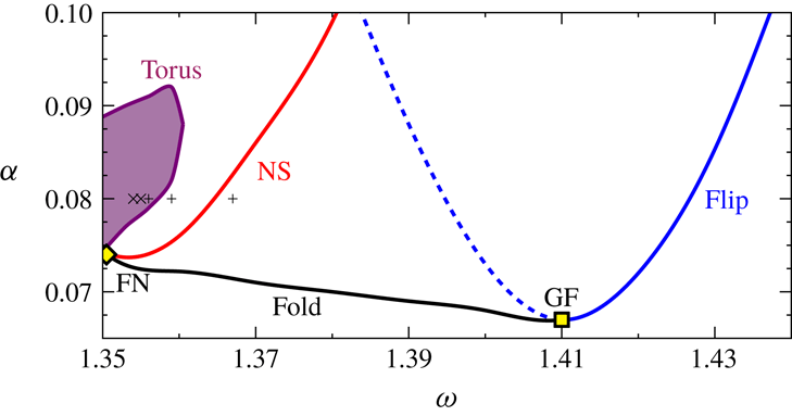
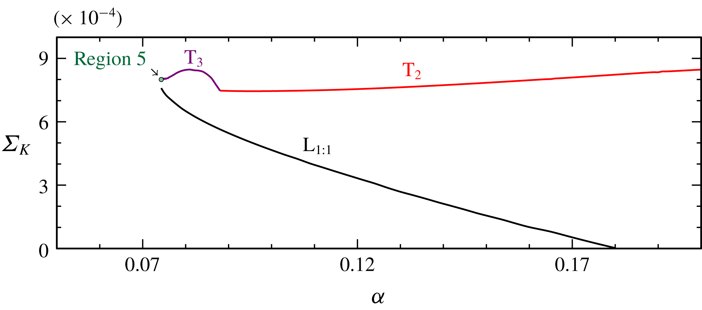
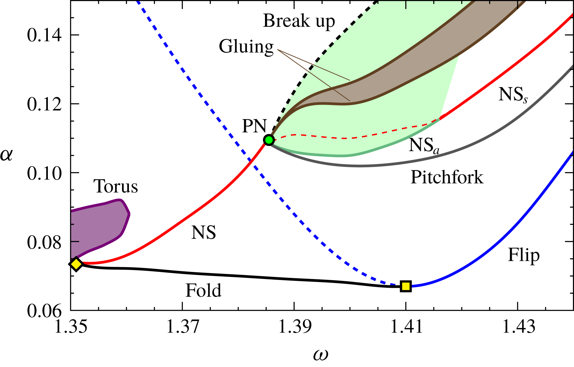
resonance tongue for the remainder of this study. This is also the resonance tongue which the experimental study of Benielli & Sommeria (Reference Benielli and Sommeria1998) primarily focused on. This tongue is the one which is least affected by neighbouring tongues near onset, and is also one of the least viscously damped tongues. Furthermore, as is evident from figure 2, the dynamics near the tip of the low-order tongues has many features in common: subcritical flip and fold-Neimark–Sacker bifurcations to the low-frequency side of the tips. In figure 5, the primary bifurcation curves found in the neighbourhood of the
 $1:1$
tongue tip are illustrated. There are a number of codimension-two points indicated in the figure. The dynamics in the neighbourhoods of some of these has been studied theoretically (Kuznetsov Reference Kuznetsov2004), but for some there are only partial known theoretical results. In the following, we describe in some detail the nonlinear dynamics in the various regions of the resonance tongue and, where possible, we relate our nonlinear simulation results to the theoretically expected dynamics.
Bifurcation curves near the tip of the
 $1:1$
resonance tongue. The flip bifurcation (blue curve) is where the basic state limit cycle period doubles; this bifurcation is supercritical along the solid blue curve and subcritical along the dashed blue curve. The fold bifurcation (black curve) is a saddle-node bifurcation of limit cycles. At the Neimark–Sacker curve (NS, red curve), the limit cycle bifurcates to a 2-torus, and at the Torus bifurcation (purple curve), the 2-torus bifurcates to a 3-torus. There are two codimension-two points: the generalized-flip (GF) and the fold-Neimark–Sacker (FN) points. The five markers are sampled solutions illustrated in figure 10.

At the tip of the tongue, located at
 $(\unicode[STIX]{x1D714},\unicode[STIX]{x1D6FC})=(1.41,0.068)$
, the flip bifurcation curve identified via Floquet analysis (Yalim et al.
Reference Yalim, Lopez and Welfert2018) is found to change from supercritical at higher
 $\unicode[STIX]{x1D714}$
to subcritical at lower
 $\unicode[STIX]{x1D714}$
. The codimension-two point at which this change happens is often called a generalized flip (GF) point (Kuznetsov Reference Kuznetsov2004). On crossing the supercritical flip bifurcation curve, the trivial basic state loses stability and a non-trivial limit cycle L
 $_{1:1}$
, whose period is equal to twice the forcing period, is spawned with amplitude growing from zero as the distance from the flip bifurcation curve increases. At the subcritical flip bifurcation, L
 $_{1:1}$
is spawned to the ‘left’ (i.e. to lower
 $\unicode[STIX]{x1D714}$
and
 $\unicode[STIX]{x1D6FC}$
) where the trivial basic state is still stable and the spawned L
 $_{1:1}$
is unstable. Near the tip, the stable L
 $_{1:1}$
coexists in this subcritical region, and we refer to the co-existing stable and unstable L
 $_{1:1}$
as upper and lower branch states.
As in Lopez et al. (Reference Lopez, Welfert, Wu and Yalim2017), the edge state technique is used to capture the unstable lower branch state. This technique is robust if the unstable state only has one unstable direction. In general, unstable edge states
 ${\mathcal{E}}$
can be approached by using convex combinations of two stable states,
 ${\mathcal{S}}_{0}$
and
 ${\mathcal{S}}_{1}$
, whose stable manifolds coincide with the unstable manifolds of the target edge state, as initial conditions and refining the weight
 $\unicode[STIX]{x1D6FE}\in (0,1)$
, such that
 $$\begin{eqnarray}{\mathcal{E}}=\unicode[STIX]{x1D6FE}{\mathcal{S}}_{0}+(1-\unicode[STIX]{x1D6FE}){\mathcal{S}}_{1}.\end{eqnarray}$$
To capture the saddle lower branch L
 $_{1:1}$
as an edge state
 ${\mathcal{E}}$
, we take the stable basic state as
 ${\mathcal{S}}_{0}$
and the stable upper branch L
 $_{1:1}$
as
 ${\mathcal{S}}_{1}$
at forcing phase 0.
As the bifurcation curve labelled ‘Fold’ in figure 5 is approached from above, the upper and lower branches L
 $_{1:1}$
coincide. The bifurcation is a saddle node of limit cycles, also known as a cyclic fold, or more simply, a fold bifurcation. This bifurcation curve also emerges from the codimension-two point GF. In the neighbourhood of GF, there is no other dynamics involved (Kuznetsov Reference Kuznetsov2004, § 9.3).
The limit cycle L
 $_{1:1}$
has broken the two reflection symmetries
 ${\mathcal{K}}_{x}$
and
 ${\mathcal{K}}_{z}$
. At any instant in time it is neither pointwise
 ${\mathcal{K}}_{x}$
nor pointwise
 ${\mathcal{K}}_{z}$
invariant, but remains pointwise
 ${\mathcal{R}}_{\unicode[STIX]{x03C0}}$
invariant. However, the broken spatial reflections have been replaced by space–time reflections. These are the half-period-flip symmetries
 ${\mathcal{P}}_{\unicode[STIX]{x1D70F}}\circ {\mathcal{K}}_{z}$
and
 ${\mathcal{P}}_{\unicode[STIX]{x1D70F}}\circ {\mathcal{K}}_{x}$
; the forcing period
 $\unicode[STIX]{x1D70F}$
is half of the response period of L
 $_{1:1}$
. Furthermore, since L
 $_{1:1}$
is
 $2\unicode[STIX]{x1D70F}$
-periodic, applying
 ${\mathcal{P}}_{\unicode[STIX]{x1D70F}}$
to it at time
 $t_{0}$
results in another
 $2\unicode[STIX]{x1D70F}$
-periodic limit cycle, which is equivalent to L
 $_{1:1}$
at
 $t_{0}+\unicode[STIX]{x1D70F}$
. In other words, there exists two initial value problem solutions L
 $_{1:1}(t)$
and L
 $_{1:1}(t+\unicode[STIX]{x1D70F})$
. Local measures such as a velocity component at a point have time series that repeat every two forcing periods (
 $2\unicode[STIX]{x1D70F}$
-periodic), whereas global measures such as
 $E_{T}$
or
 $E_{K}$
are
 $\unicode[STIX]{x1D70F}$
-periodic as a consequence of the half-period-flip symmetries.
6 Dynamics in the subcritical region of the
$\mathbf{1}\boldsymbol{ : }\mathbf{1}$
tongue

In the subcritical region near the tip of the tongue (i.e. in the neighbourhood of the generalized flip codimension-two point GF), the stable basic state, the stable (upper branch) L
 $_{1:1}$
and the unstable (lower branch) L
 $_{1:1}$
coexist. Increasing
 $\unicode[STIX]{x1D6FC}$
and/or lowering
 $\unicode[STIX]{x1D714}$
, the upper branch L
 $_{1:1}$
becomes unstable via a Neimark–Sacker bifurcation in which a stable quasi-periodic state
 $\text{T}_{2}$
emerges. This
 $\text{T}_{2}$
is setwise
 ${\mathcal{G}}$
symmetric. The Neimark–Sacker curve (labelled NS in figure 5) meets the fold curve emanating from the generalized flip point (GF) at another codimension-two fold-Neimark–Sacker bifurcation point, labelled FN in figure 5. It is one of the codimension-two points that only has partially known theoretical results (Kuznetsov Reference Kuznetsov2004, § 9.1, case 9).
6.1 Fold-Neimark–Sacker dynamics
The fold-Neimark–Sacker bifurcation is sometimes called the Hopf saddle node for maps bifurcation. It has been studied by Broer, Simó & Vitolo (Reference Broer, Simó and Vitolo2008) in a low-dimensional model problem that was designed to be as ‘generic as possible’. The model was constructed by perturbing the Poincaré map of the truncated normal form for the Hopf-saddle-node bifurcation. In essence, the Hopf-saddle-node bifurcation is treated as being the stroboscopic map of the fold-Neimark–Sacker bifurcation. As such, steady states and limit cycles of the Hopf-saddle-node bifurcation correspond to limit cycles and 2-tori of the fold-Neimark–Sacker bifurcation, and the strobes of those limit cycles and 2-tori are fixed points and cycles in the approximating map. But complications set in due to possible resonances when the frequencies of the 2-tori are in low-order rational ratios. Broer et al. (Reference Broer, Simó and Vitolo2008) provide several conjectures based on numerical studies of their model problem that involve various bifurcations of limit cycles and 2-tori, yielding a cascade of bifurcations of 2-tori, and heteroclinic and homoclinic behaviour. The Hopf-saddle-node bifurcation scenario on which their model was based is the one that includes the complex dynamics associated with the breaking of a heteroclinic connection. The nonlinear dynamics in the neighbourhood of such a Hopf-saddle-node bifurcation has been studied numerically and experimentally in short aspect-ratio Taylor–Couette flows (Lopez, Marques & Shen Reference Lopez, Marques and Shen2004; Abshagen et al. Reference Abshagen, Lopez, Marques and Pfister2005). Here, we find that much of the simpler dynamics in the neighbourhood of the fold-Neimark–Sacker bifurcation FN indicated in figure 5 can be diagnosed along these same lines, and as in all Hopf-saddle-node and fold-Neimark–Sacker bifurcations that have been studied, the complex dynamics is very much case dependent, but intrinsically associated with the heteroclinic region. In the following, we describe in some detail such dynamics.
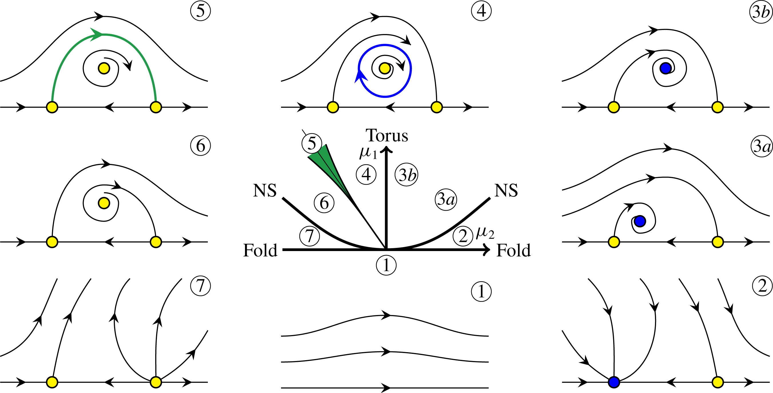
Schematic of the Hopf-saddle-node bifurcation, which is used to discuss the fold-Neimark–Sacker (FN) bifurcation. The central plot is the bifurcation diagram, and the surrounding plots are typical phase portraits in the various sections of the bifurcation diagram, labelled 1–7. In these phase portraits, the symbols on the horizontal axis are stable (blue) or unstable (yellow) equilibria, which correspond to the upper and lower branch L
 $_{1:1}$
limit cycles in the full problem.

Figure 6 is a schematic of a Hopf-saddle-node bifurcation which we adopt to discuss the dynamics in the neighbourhood of the fold-Neimark–Sacker point FN in figure 5. The FN point is at the origin of the bifurcation diagram,
 $(\unicode[STIX]{x1D707}_{1},\unicode[STIX]{x1D707}_{2})=(0,0)$
, where the coordinates
 $\unicode[STIX]{x1D707}_{1}$
and
 $\unicode[STIX]{x1D707}_{2}$
are the variables in the codimension-two normal form. These are related to the two variables our full problem,
 $\unicode[STIX]{x1D714}$
and
 $\unicode[STIX]{x1D6FC}$
, by linear transformations near the point FN. The bifurcation diagram has a number of bifurcation curves that divide the
 $(\unicode[STIX]{x1D707}_{1},\unicode[STIX]{x1D707}_{2})$
space into various regions, labelled 1–7. Typical phase portraits in these regions are provided in the figure. In these phase portraits, the symbols on the horizontal axis are stable (blue) or unstable (yellow) equilibria, which correspond to the upper and lower branch L
 $_{1:1}$
limit cycles in the full problem. In region 1 (
 $\unicode[STIX]{x1D707}_{1}<0$
), there are no solutions nearby in phase space and all initial conditions evolve away from this region of phase space. In the full problem the evolutions end up at the stable basic state, which is far removed from the neighbourhood of the fold-Neimark–Sacker bifurcation in phase space.
Crossing the fold bifurcation curve from region 1 into region 2, the fold bifurcation leads to the creation of the upper and lower branch L
 $_{1:1}$
. Crossing the Neimark–Sacker curve NS from region 2 to region 3, the stable upper branch L
 $_{1:1}$
loses stability and spawns a stable 2-torus
 $\text{T}_{2}$
. In the phase portraits for regions 3a and 3b, this 2-torus is indicated as a (blue) equilibrium off the axis. The way to interpret the nature of the equilibria in the phase portraits is such that equilibria on the axis have one frequency (corresponding to
 $\unicode[STIX]{x1D714}/2$
since the L
 $_{1:1}$
are subharmonic); equilibria off the axis correspond to 2-tori and have an additional frequency (associated with rotations of the equilibria around the axis). The second frequency varies along the Neimark–Sacker curve NS, and may be in a rational ratio with the first frequency (
 $\unicode[STIX]{x1D714}/2$
) at various points along the curve. From such points emerge Arnold tongues into region 3 in which the flow is phase locked.
Schematic of the transverse across the green wedge-shaped region 5 in figure 6. The blue and green curves are the stable and unstable manifolds of the two saddle states (yellow symbols), that intersect transversely.

Crossing from region 3 into region 4, the curve labelled ‘Torus’ is crossed, at which the 2-torus loses stability (it goes from being blue to yellow) and a stable (blue) invariant circle is spawned in the phase portrait for region 4. This invariant circle has three frequencies associated with it: two are inherited from the 2-torus and the third is new corresponding to cycling around the blue circle. This indicates the birth of a 3-torus
 $\text{T}_{3}$
. Below we give descriptions of numerical solutions exhibiting 3-torus dynamics in the corresponding parameter region in figure 5. The dynamics in region 5 is not smooth due to various resonances, as suggested by the model case study in Broer et al. (Reference Broer, Simó and Vitolo2008). In the Hopf-saddle-node normal form, the invariant circle becomes heteroclinic to the two unstable equilibria on the axis (the green curve in the region 5 phase portrait). Even for the Hopf-saddle-node bifurcation, this heteroclinic connection does not persist if higher-order terms in the normal form are included. Typically, the higher-order terms result in the stable and unstable manifolds emanating from the unstable equilibria on the axis intersecting transversely instead of coinciding. This is illustrated in figure 7. The wedge-shaped region 5 in green demarcates the region where the transverse intersections occur. It is in this region that very complicated dynamics occurs, some of which we describe below. Continuing from region 5 into regions 6 and 7, all states in the phase space neighbourhood of the fold-Neimark–Sacker bifurcation are unstable, and so all initial conditions eventually evolve away from this part of phase space.
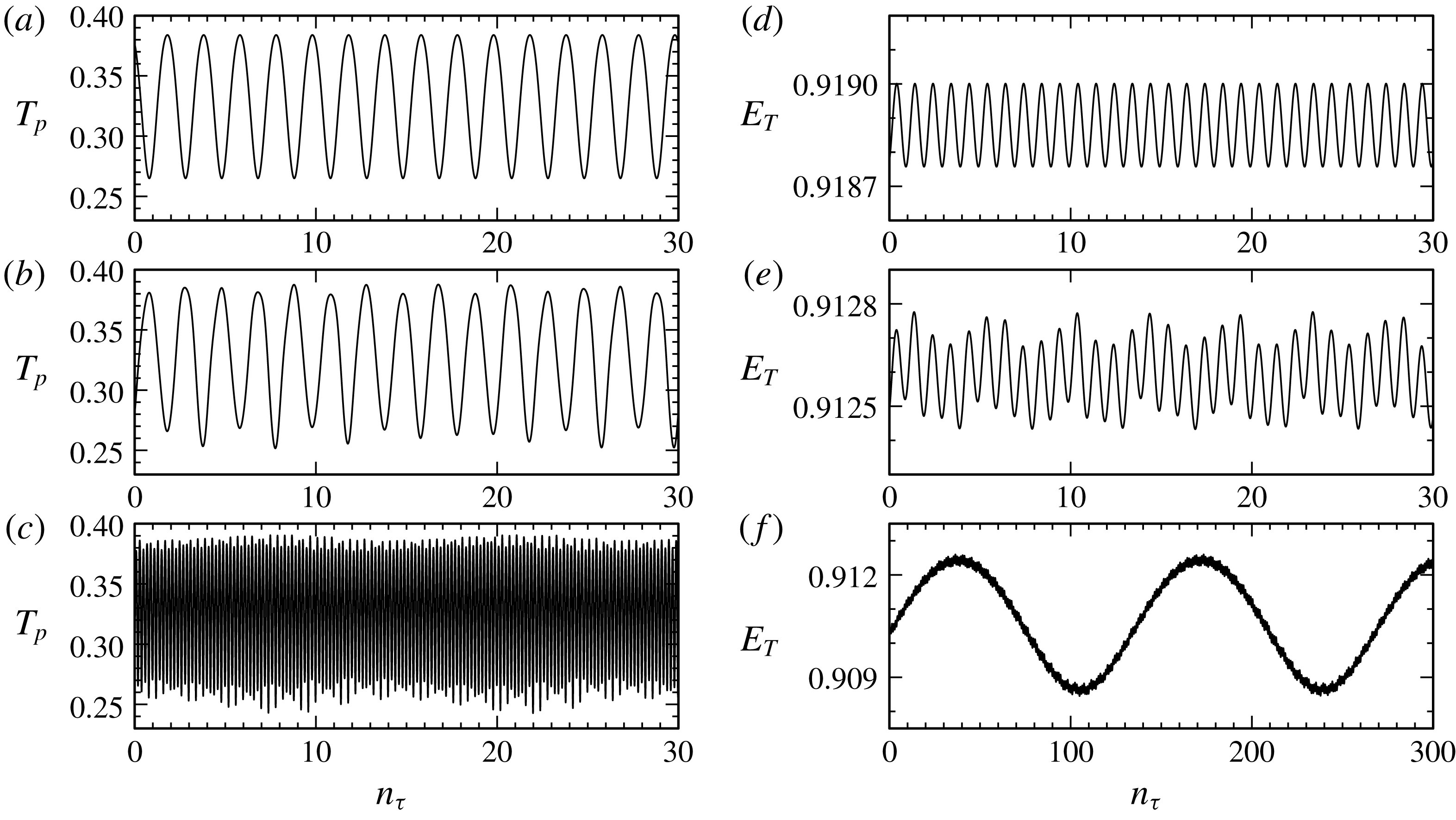
Time series of the temperature at
 $(x_{p},z_{p})=(1/\sqrt{8},1/\sqrt{8})$
,
 $T_{p}$
(a–c) and the normalized thermal
 ${\mathcal{L}}^{2}$
measure
 $E_{T}$
(d–f) for (a,d) L
 $_{1:1}$
at
 $\unicode[STIX]{x1D714}=1.367$
, (b,e) T
 $_{2}$
at
 $\unicode[STIX]{x1D714}=1.359$
and (c,f) T
 $_{3}$
at
 $\unicode[STIX]{x1D714}=1.356$
, all with
 $\unicode[STIX]{x1D6FC}=0.08$
, corresponding to the ‘
 $+$
’ marks in figure 5.

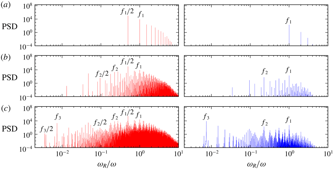
Frequency spectra of the time series shown in figure 8. The angular response frequency
 $\unicode[STIX]{x1D714}_{R}$
has been normalized by the forcing frequency
 $\unicode[STIX]{x1D714}$
.

6.2 Torus bifurcation to
$\text{T}_{3}$

Figure 5 includes ‘
 $+$
’ markers, these indicate the
 $(\unicode[STIX]{x1D714},\unicode[STIX]{x1D6FC})$
locations of some sample states whose time series are shown in figure 8. Time is shown in units of
 $n_{\unicode[STIX]{x1D70F}}$
, the number of forcing periods
 $\unicode[STIX]{x1D70F}=2\unicode[STIX]{x03C0}/\unicode[STIX]{x1D714}$
. All are shown at
 $\unicode[STIX]{x1D6FC}=0.08$
and the variation in
 $\unicode[STIX]{x1D714}$
corresponds to a traverse through the NS and Torus bifurcation curves. For each case, the time series on the left is of
 $T_{p}$
, the temperature at the point
 $(x_{p},z_{p})=(1/\sqrt{8},1/\sqrt{8})$
(a local measure). The one on the right is of the normalized thermal
 ${\mathcal{L}}^{2}$
measure
 $E_{T}$
(a global measure). The first case at
 $\unicode[STIX]{x1D714}=1.367$
is the upper branch limit cycle L
 $_{1:1}$
. As described earlier, it is a subharmonic response so that the local measure is
 $2\unicode[STIX]{x1D70F}$
-periodic, but it is setwise
 ${\mathcal{G}}$
symmetric so its global measure is
 $\unicode[STIX]{x1D70F}$
-periodic. The power spectral densities (PSD) of these time series are shown in figure 9(a). The spectrum of
 $E_{T}$
shows a single peak at
 $\unicode[STIX]{x1D714}_{R}/\unicode[STIX]{x1D714}=f_{1}=1.0$
, plus harmonics, whereas that of
 $T_{p}$
also shows a (stronger) peak at
 $\unicode[STIX]{x1D714}_{R}/\unicode[STIX]{x1D714}=f_{1}/2$
, plus harmonics. The next state at
 $\unicode[STIX]{x1D714}=1.359$
is to the low-
 $\unicode[STIX]{x1D714}$
side of the NS curve. It is a 2-torus
 $\text{T}_{2}$
that was spawned at the Neimark–Sacker bifurcation where L
 $_{1:1}$
loses stability. The time series of
 $\text{T}_{2}$
are very similar to those of L
 $_{1:1}$
with a small amplitude modulation. Together with the corresponding spectra, we see that this modulation frequency is
 $f_{2}\approx 0.223f_{1}$
. The
 $E_{T}$
spectrum of
 $\text{T}_{2}$
consists of peaks at these two frequencies plus their linear combinations. The
 $T_{p}$
spectrum has many more peaks, corresponding to
 $f_{1}/2$
,
 $f_{2}/2$
and all their linear combinations. This is evidence that
 $\text{T}_{2}$
is also setwise
 ${\mathcal{G}}$
symmetric. The third case at
 $\unicode[STIX]{x1D714}=1.356$
is to the low-
 $\unicode[STIX]{x1D714}$
side of the Torus curve. On crossing the Torus curve,
 $\text{T}_{2}$
loses stability and a 3-torus
 $\text{T}_{3}$
is spawned. The
 $T_{p}$
time series shows multiple frequencies, but the
 $E_{T}$
time series of
 $\text{T}_{3}$
is essentially that of
 $\text{T}_{2}$
with a very large amplitude (approximately a factor of 10) low-frequency modulation. The corresponding
 $E_{T}$
spectrum of
 $\text{T}_{3}$
consists of peaks at
 $f_{1}$
and
 $f_{2}$
(just like that of
 $\text{T}_{2}$
), together with a very low-frequency peak at
 $f_{3}\approx 0.0075f_{1}$
(corresponding to a period of approximately 133
 $\unicode[STIX]{x1D70F}$
), and all their linear combinations. The spectrum of the local measure
 $T_{p}$
has many more peaks as it consists of all the linear combinations of
 $f_{1}/2$
,
 $f_{2}/2$
and
 $f_{3}/2$
.
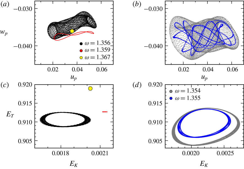
Local and global strobe maps of the flows with
 $\unicode[STIX]{x1D6FC}=0.08$
at the specified forcing frequency
 $\unicode[STIX]{x1D714}$
, showing the strobed behaviour of 1-tori, 2-tori and 3-tori as
 $\unicode[STIX]{x1D714}$
is decreased. The states shown in (a,c) correspond to the
 $+$
markers in figure 5 and those in (b,d) to the
 $\times$
markers.

Figure 10 shows strobe maps using both local (panel
 $a$
) and global (panel
 $c$
) quantities of the three states just described above (corresponding to the
 $+$
markers in figure 5). The local map uses the horizontal and vertical components of velocity at the point
 $(x_{p},z_{p})=(1/\sqrt{8},1/\sqrt{8})$
every two forcing periods at forcing phase
 $\unicode[STIX]{x03C0}$
. The global map strobes the kinetic and thermal global measures, given in (2.3), also every two forcing periods and at a half-period phase shift. The first state is L
 $_{1:1}$
at
 $\unicode[STIX]{x1D714}=1.367$
. Its strobe map is a point (yellow circular symbol). The next state is
 $\text{T}_{2}$
at
 $\unicode[STIX]{x1D714}=1.359$
. Its strobe map is a cycle (closed red loop), which is clearly seen in the local map but requires a significant zoom in to be clearly seen in the global map. The third state is
 $\text{T}_{3}$
at
 $\unicode[STIX]{x1D714}=1.356$
. The global strobe map of
 $\text{T}_{3}$
is the black doughnut-shaped structure, typical of a 2-torus; its structure in the local strobe map is also a 2-torus. Figure 10(b,d) shows the local and global strobe maps for two other
 $\text{T}_{3}$
states. These are indicated by the ‘
 $\times$
’ markers in figure 5 at slightly smaller
 $\unicode[STIX]{x1D714}=1.355$
and
 $1.354$
. Their strobe maps show how they rapidly expand in phase space with very small decreases in
 $\unicode[STIX]{x1D714}$
. Also, the
 $\unicode[STIX]{x1D714}=1.355$
case is nearly phase locked; the strobe map is a convoluted cycle on a 2-torus.
Bifurcation diagram for
 $\unicode[STIX]{x1D714}=1.35$
.

6.3 Homoclinic-doubling cascade on the
$T_{3}$

We now explore some of the dynamics inside the region enclosed by the Torus curve (shaded purple in figure 5). We begin by fixing
 $\unicode[STIX]{x1D714}=1.35$
. Figure 11 is a bifurcation diagram at this
 $\unicode[STIX]{x1D714}$
, using the temporal standard deviation in the kinetic energy,
 $\unicode[STIX]{x1D6F4}_{K}$
, as a measure of the state. The basic state has
 $\unicode[STIX]{x1D6F4}_{K}=0$
. It loses stability at
 $\unicode[STIX]{x1D6FC}\approx 0.181$
in a subcritical flip bifurcation, spawning an unstable limit cycle L
 $_{1:1}$
to lower
 $\unicode[STIX]{x1D6FC}$
. For larger
 $\unicode[STIX]{x1D6FC}$
, the flow evolves to the quasi-periodic
 $\text{T}_{2}$
, which we have continued down to smaller
 $\unicode[STIX]{x1D6FC}$
. At
 $\unicode[STIX]{x1D6FC}\approx 0.089$
,
 $\text{T}_{2}$
loses stability at the Torus bifurcation, and 3-torus
 $\text{T}_{3}$
is spawned. Using the stable
 $\text{T}_{2}$
and
 $\text{T}_{3}$
, together with the stable basic state, we have used the edge state technique to capture the unstable L
 $_{1:1}$
. At
 $\unicode[STIX]{x1D6FC}\approx 0.074426$
, the
 $\text{T}_{3}$
begins a cascade of bifurcations which are described below in some detail. This essentially corresponds to entering region 5 marked in the schematic of the Hopf-saddle-node bifurcation in figure 6.
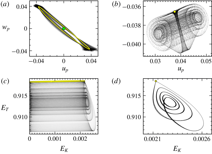
Figure 12 illustrates some characteristics of a state in the above-mentioned region 5. It shows the local phase portrait (figure 12
a), using the two velocity components at the point
 $(x_{p},z_{p})=(1/\sqrt{8},1/\sqrt{8})$
and the global phase portrait (figure 12
c), using
 $E_{T}$
and
 $E_{K}$
, of the basic state (green dot in the local phase portrait), the unstable L
 $_{1:1}$
(yellow cycle in the local and global phase portraits; note however that
 $E_{T}$
of L
 $_{1:1}$
is essentially time invariant), and a complicated state that resides in region 5 (black cloud of dots). Further insight is gained by examining the strobed phase portraits, shown in figure 12(b,d). In the strobe maps, the limit cycle L
 $_{1:1}$
is simply a point (yellow dot), and the complicated state in the global strobe map is a thin 2-torus with five loops and in the local strobe map it appears as a wide 2-torus structure with five scrolls. Furthermore, this
 $\text{T}_{3}$
is very close to forming a homoclinic connection to the unstable L
 $_{1:1}$
.
(a) Local phase portraits of the basic state (green dot), the unstable lower branch L
 $_{1:1}$
(yellow cycle computed using the edge state technique) and the stable attractor (black cloud), and (b) the corresponding strobe map (strobed every two forcing periods at forcing phase
 $\unicode[STIX]{x03C0}/2$
), in which L
 $_{1:1}$
is a single (yellow) dot, and the stable attractor is in black, all at
 $(\unicode[STIX]{x1D714},\unicode[STIX]{x1D6FC})=(1.35,0.0743178)$
. (c,d) Illustrate the global data associated with (a,b). Note that the basic state is not shown in (c); it is located at
 $(E_{K},E_{T})=(0,1)$
.

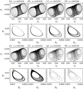
Local and global strobe maps (strobed every two forcing periods at forcing phase
 $\unicode[STIX]{x03C0}/2$
) for
 $\unicode[STIX]{x1D714}=1.35$
and
 $\unicode[STIX]{x1D6FC}$
as indicated, illustrating states in the period-doubling cascade. The yellow marker corresponds to the strobed unstable L
 $_{1:1}$
, determined using the edge state technique.

The
 $\text{T}_{3}$
for
 $\unicode[STIX]{x1D714}=1.35$
and
 $\unicode[STIX]{x1D6FC}\in [0.07443,0.089]$
exhibits behaviour which we describe as having an
 $\ell =1$
loop. Reducing the forcing amplitude just below
 $\unicode[STIX]{x1D6FC}\approx 0.07442$
, the global strobe map shows that
 $\text{T}_{3}$
has
 $\ell =2$
loops. In a sense, there has been a period doubling of the
 $\text{T}_{3}$
. Further reducing
 $\unicode[STIX]{x1D6FC}$
below approximately
 $0.074374$
, there is another period doubling resulting in an
 $\ell =4$
 $\text{T}_{3}$
, and an
 $\ell =8$
 $\text{T}_{3}$
at
 $\unicode[STIX]{x1D6FC}\approx 0.074365$
. Further doublings were not resolved in this neighbourhood. Examples of
 $\text{T}_{3}$
with
 $\ell =1$
, 2, 4 and 8 are shown in figure 13(a–d), which gives both the local and global strobe maps of the
 $\text{T}_{3}$
(they also include the unstable L
 $_{1:1}$
obtained using the edge state technique, indicated as a yellow dot). The strobe maps for smaller
 $\unicode[STIX]{x1D6FC}$
(figure 13
e–h) generally did not show distinct loops or scrolls, except for some very narrow windows in
 $\unicode[STIX]{x1D6FC}$
where an
 $\ell =6$
 $\text{T}_{3}$
at
 $\unicode[STIX]{x1D6FC}=0.074359$
and an
 $\ell =5$
 $\text{T}_{3}$
at
 $\unicode[STIX]{x1D6FC}=0.074350$
were detected. The start of a second period-doubling cascade with
 $\ell =3\rightarrow \ell =6$
at
 $\unicode[STIX]{x1D6FC}\approx 0.07434$
was also found. This behaviour of the strobe maps is very reminiscent of the behaviour of the logistic map (May Reference May1976).
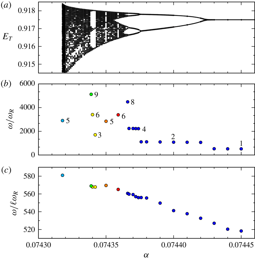
(a) Variation with
 $\unicode[STIX]{x1D6FC}$
of
 $E_{T}$
strobed every two forcing periods at forcing phase
 $\unicode[STIX]{x03C0}/2$
for
 $\unicode[STIX]{x1D714}=1.35$
, (b) response period relative to the forcing period,
 $\unicode[STIX]{x1D714}/\unicode[STIX]{x1D714}_{R}$
, in the periodic windows in (a), with the integer
 $\ell$
related to the logistic map like period-doubling cascade, and (c)
 $\unicode[STIX]{x1D714}/\ell \unicode[STIX]{x1D714}_{R}$
. See supplementary movie 2, which shows how the local and global strobed phase portraits (shown in figure 13) vary with
 $\unicode[STIX]{x1D6FC}$
.

We further explore the logistic map-like behaviour of the strobe maps by taking a Poincaré-like section of the global strobe map. Of course, the strobe map is a discrete-time map and so we cannot simply take a Poincaré section of it. Instead, we define a transverse section, give it a little thickness and record
 $E_{T}$
whenever the strobe map is within this thin transverse rectangular section. The strobe map was iterated (i.e. the flow was simulated) for up to
 $10^{6}$
forcing periods for each value of
 $\unicode[STIX]{x1D6FC}$
(124 values of
 $\unicode[STIX]{x1D6FC}\in [0.0743178,0.074520]$
). The results (discarding the early transients) are shown in figure 14(a). The similarity to the logistic map is striking. Supplementary movie 2 animates the 124 cases in this small range in
 $\unicode[STIX]{x1D6FC}$
, with each frame corresponding to a different value of
 $\unicode[STIX]{x1D6FC}$
, and consisting of the local and global strobe maps at that
 $\unicode[STIX]{x1D6FC}$
, and a vertical line at the
 $\unicode[STIX]{x1D6FC}$
value of the plot in figure 14(a). At several of the
 $\unicode[STIX]{x1D6FC}$
values where the strobe maps have distinct
 $\ell$
loops/scrolls, we plot in figure 14(b) the period corresponding to the very low frequency in the
 $\text{T}_{3}$
, and in figure 14(c) this period is divided by
 $\ell$
, giving essentially the averaged period
 $1/f_{3}$
over the
 $\ell$
loops. This averaged period
 $1/f_{3}$
grows linearly with decreasing
 $\unicode[STIX]{x1D6FC}$
.
The logistic map-like dynamics just described also has much in common with what is theoretically expected in a so-called homoclinic-doubling cascade (Oldeman, Krauskopf & Champneys Reference Oldeman, Krauskopf and Champneys2000), in which an entire period-doubling cascade collides with a saddle equilibrium. In period-doubling cascades that do not involve homoclinic collisions, the parameter values at which the period-doubling bifurcations occur follow a self-similar scaling given by the Feigenbaum constant (Feigenbaum Reference Feigenbaum1978). In contrast, for the homoclinic-doubling cascade, the scaling constants depend on the eigenvalues of the saddle equilibrium. While Oldeman et al. (Reference Oldeman, Krauskopf and Champneys2000) studied a system of three ordinary differential equations with quadratic nonlinearity that was constructed to satisfy conditions for the existence of a homoclinic-doubling cascade, they concluded that such a cascade is a generic mechanism that should be found in many physical systems. We believe that the cascade we have found is the first to be reported in a hydrodynamic system.
7 Dynamics associated with symmetry breaking and restoring
So far, all of the flows described in the
 $1:1$
tongue have been pointwise
 ${\mathcal{R}}_{\unicode[STIX]{x03C0}}$
invariant and setwise
 ${\mathcal{G}}$
invariant. Keeping our focus within this tongue (figure 5), we now explore how these symmetries are broken and restored. We begin by fixing
 $\unicode[STIX]{x1D714}=1.41$
, which is very close to the frequency at the tip of the
 $1:1$
tongue, and increase
 $\unicode[STIX]{x1D6FC}$
. Upon increasing
 $\unicode[STIX]{x1D6FC}$
across the tongue at
 $\unicode[STIX]{x1D6FC}\approx 0.066$
, the subharmonic L
 $_{1:1}$
is spawned, as described earlier. As was noted in § 3, for any state
 ${\mathcal{S}}$
that is not synchronous with the forcing, there also exists a conjugate state
 ${\mathcal{P}}_{\unicode[STIX]{x1D70F}}({\mathcal{S}})$
. This is the case for L
 $_{1:1}$
and all states that bifurcate from it. Up to now, this has not been dynamically important, but it will be in some parameter regimes which we now explore.
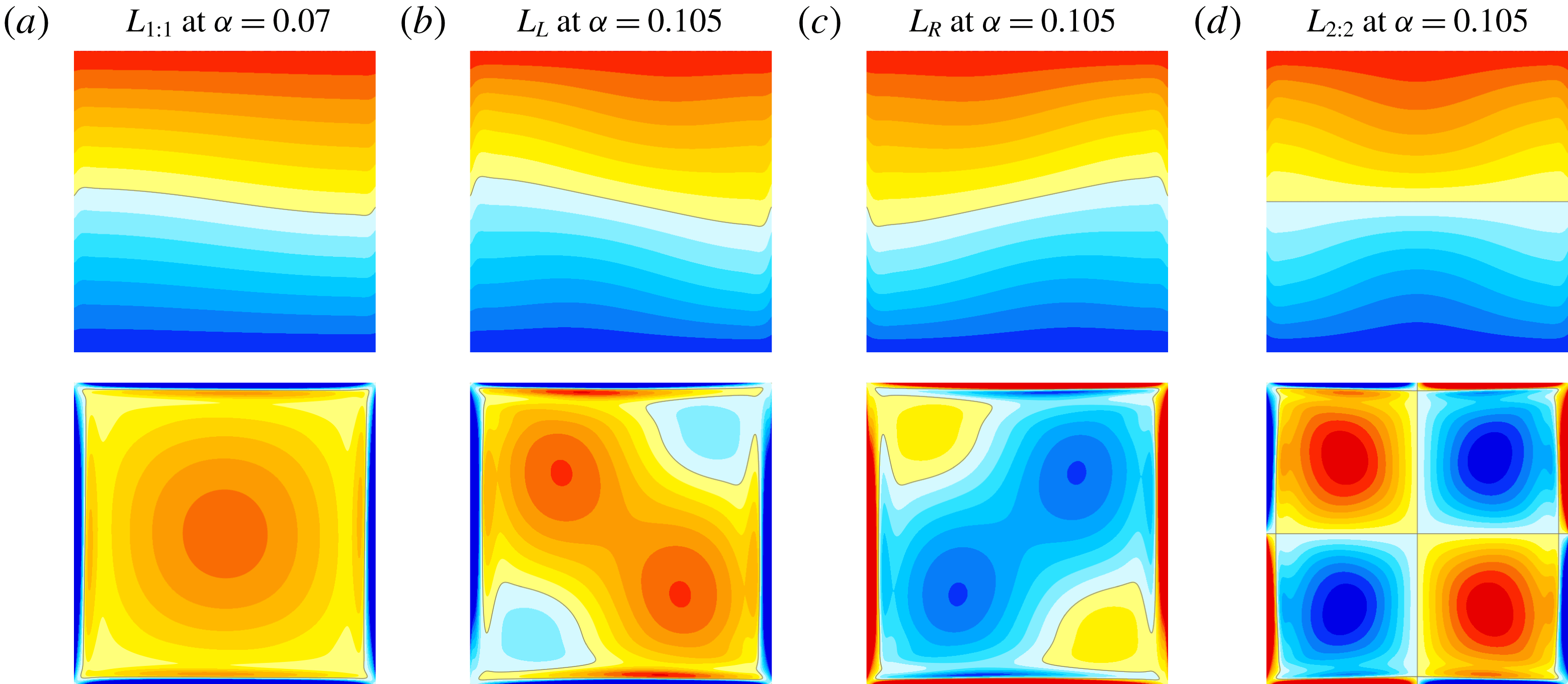
Snapshots of the temperature and vorticity for subharmonic limit cycles at
 $\unicode[STIX]{x1D714}=1.41$
: (a) L
 $_{1:1}$
at
 $\unicode[STIX]{x1D6FC}=0.07$
, (b,c) L
 $_{L}$
and L
 $_{R}$
at
 $\unicode[STIX]{x1D6FC}=0.105$
, and (d) L
 $_{2:2}$
at
 $\unicode[STIX]{x1D6FC}=0.105$
. The temperature snapshots are at forcing phase
 $3\unicode[STIX]{x03C0}/2$
whereas the vorticity is shown at
 $\unicode[STIX]{x03C0}/2$
. Supplementary movie 3 animates the temperature and vorticity of the four limit cycles over two forcing periods.

Increasing
 $\unicode[STIX]{x1D6FC}$
past
 $0.101$
, L
 $_{1:1}$
loses stability at a pitchfork bifurcation breaking the half-period-flip symmetry, i.e. the setwise
 ${\mathcal{G}}$
invariance, where a pair of symmetrically related limit cycles, L
 $_{L}$
and L
 $_{R}$
, appear. Applying either
 ${\mathcal{K}}_{x}$
or
 ${\mathcal{K}}_{z}$
to one results in the other,
 $$\begin{eqnarray}{\mathcal{K}}_{x}\,\text{L}_{L}(x,z,t)=\text{L}_{R}(x,z,t)\quad \text{and}\quad {\mathcal{K}}_{z}\,\text{L}_{L}(x,z,t)=\text{L}_{R}(x,z,t).\end{eqnarray}$$
Figure 15 illustrates snapshots of the temperature and vorticity of L
 $_{1:1}$
at
 $\unicode[STIX]{x1D6FC}=0.066$
, and L
 $_{L}$
, L
 $_{R}$
and L
 $_{2:2}$
at
 $\unicode[STIX]{x1D6FC}=0.105$
(supplementary movie 3 animates these over two forcing periods); these states are all pointwise
 ${\mathcal{R}}_{\unicode[STIX]{x03C0}}$
invariant. Note that L
 $_{2:2}$
is unstable. It was computed by restricting the simulations to the
 ${\mathcal{G}}$
symmetric subspace.
In fact, much of the dynamics we will describe in this section entails interactions that involve unstable states, such as L
 $_{2:2}$
. Fortunately, many of these are stable in symmetry subspaces, and so we now explore the dynamics restricted to the various symmetry subspaces before putting it all together in the full space.
7.1 Dynamics restricted to the
${\mathcal{G}}$
and
${\mathcal{K}}_{z}$
subspaces


L
 $_{2:2}$
is pointwise
 ${\mathcal{G}}$
invariant. Fixing
 $\unicode[STIX]{x1D714}=1.41$
and computing in the
 ${\mathcal{G}}$
subspace, L
 $_{2:2}$
is found to bifurcate subharmonically (so it is
 $2\unicode[STIX]{x1D70F}$
periodic) from the base state by
 $\unicode[STIX]{x1D6FC}\approx 0.084$
, which is very close to the forcing amplitude predicted by Floquet analysis,
 $\unicode[STIX]{x1D6FC}\approx 0.0831$
(Yalim et al.
Reference Yalim, Lopez and Welfert2018). It remains stable up to
 $\unicode[STIX]{x1D6FC}\approx 0.155$
. However, if the simulations are only restricted to the
 ${\mathcal{K}}_{z}$
subspace, it loses stability at
 $\unicode[STIX]{x1D6FC}\approx 0.087$
via a
 ${\mathcal{K}}_{x}$
-symmetry-breaking Neimark–Sacker bifurcation. The new frequency
 $f_{2}$
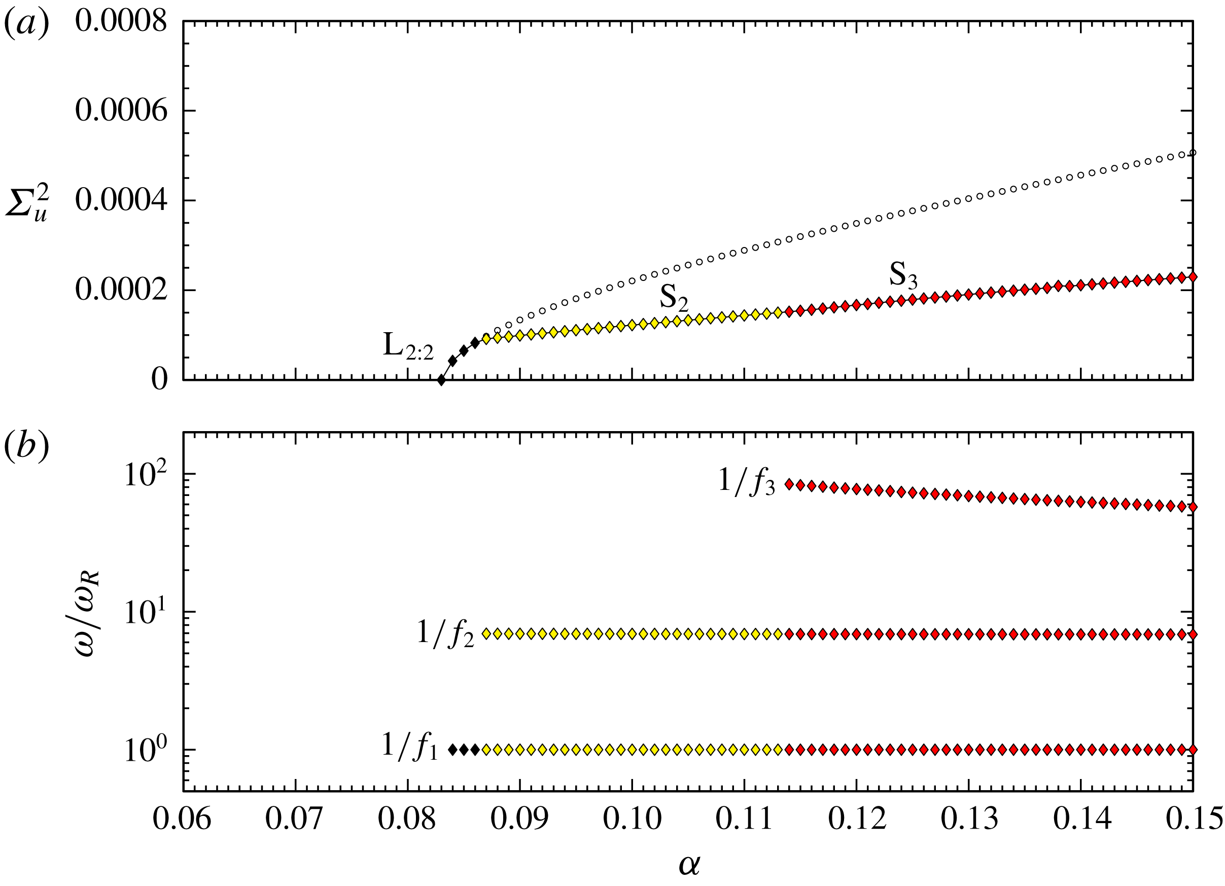
is approximately an order of magnitude smaller than the forcing frequency,
 $1/f_{2}\approx 7$
, and corresponds to an internal sloshing state that modulates the L
 $_{2:2}$
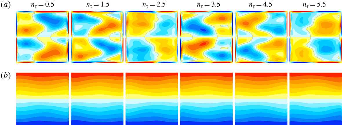
oscillation. Figure 16 shows a few snapshots of the temperature and vorticity of the sloshing state, S
 $_{2}$
, at
 $\unicode[STIX]{x1D6FC}=0.111$
(supplementary movie 4 shows the temporal evolution over six forcing periods). S
 $_{2}$
loses stability at
 $\unicode[STIX]{x1D6FC}\approx 0.114$
at a secondary Neimark–Sacker bifurcation that spawns a 3-torus, S
 $_{3}$
, which inherits the two frequencies of S
 $_{2}$
and has a new much lower third frequency, approximately another order of magnitude smaller. Figure 17 shows the variations with
 $\unicode[STIX]{x1D6FC}$
of the variance of the horizontal velocity
 $\unicode[STIX]{x1D6F4}_{u}^{2}$
at the point
 $(x_{p},z_{p})=(1/\sqrt{8},1/\sqrt{8})$
and the number of forcing periods
 $\unicode[STIX]{x1D714}/\unicode[STIX]{x1D714}_{R}$
associated with the primary
 $E_{T}$
response frequencies of L
 $_{2:2}$
, S
 $_{2}$
and S
 $_{3}$
for
 $\unicode[STIX]{x1D714}=1.41$
.
Snapshots of (a) the vorticity and (b) the temperature of S
 $_{2}$
at
 $\unicode[STIX]{x1D714}=1.41$
and
 $\unicode[STIX]{x1D6FC}=0.111$
shown at six consecutive forcing periods at phase
 $\unicode[STIX]{x03C0}$
. Supplementary movie 4 shows the corresponding animations over the six forcing periods.

Variations with
 $\unicode[STIX]{x1D6FC}$
at
 $\unicode[STIX]{x1D714}=1.41$
of (a) the variance of the horizontal velocity
 $\unicode[STIX]{x1D6F4}_{u}^{2}$
at the point
 $(x_{p},z_{p})=(1/\sqrt{8},1/\sqrt{8})$
, computed in the
 ${\mathcal{K}}_{z}$
symmetric subspace, and (b) the number of forcing periods corresponding to the
 $E_{T}$
response frequencies of L
 $_{2:2}$
(
 $f_{1}$
), S
 $_{2}$
(
 $f_{1}$
,
 $f_{2}$
) and S
 $_{3}$
(
 $f_{1}$
,
 $f_{2}$
,
 $f_{3}$
). The part of the L
 $_{2:2}$
branch with open circles is unstable in the
 ${\mathcal{K}}_{z}$
, but is stable in the
 ${\mathcal{G}}$
subspace.

7.2 Dynamics in the
${\mathcal{R}}_{\unicode[STIX]{x03C0}}$
subspace

We now consider what happens in the
 ${\mathcal{R}}_{\unicode[STIX]{x03C0}}$
invariant subspace. L
 $_{L}$
and L
 $_{R}$
which bifurcated from L
 $_{1:1}$
at the pitchfork bifurcation at
 $\unicode[STIX]{x1D6FC}\approx 0.084$
are
 ${\mathcal{R}}_{\unicode[STIX]{x03C0}}$
invariant, as is L
 $_{1:1}$
. In the
 ${\mathcal{R}}_{\unicode[STIX]{x03C0}}$
subspace they remain stable until
 $\unicode[STIX]{x1D6FC}\approx 0.1208$
, where they lose stability at a Neimark–Sacker bifurcation NS
 $_{s}$
. A 2-torus pair, Q
 $_{L}$
and Q
 $_{R}$
, are spawned and are
 ${\mathcal{G}}$
symmetry conjugates. The period associated with the second frequency acquired at NS
 $_{s}$
is approximately 400 forcing periods near onset and suddenly becomes unbounded as
 $\unicode[STIX]{x1D6FC}$
is increased. This second frequency corresponds to a slow drift toward and away from the
 ${\mathcal{G}}$
symmetry subspace, and at
 $\unicode[STIX]{x1D6FC}=\unicode[STIX]{x1D6FC}_{G1}\approx 0.125536$
, Q
 $_{L}$
and Q
 $_{R}$
each become homoclinic to the saddle L
 $_{1:1}$
which resides in the
 ${\mathcal{G}}$
subspace. For
 $\unicode[STIX]{x1D6FC}>\unicode[STIX]{x1D6FC}_{G1}$
, a single setwise
 ${\mathcal{G}}$
invariant 2-torus, Q, results from the homoclinic gluing (Glendinning Reference Glendinning1984). The homoclinic gluing bifurcation occurs when two symmetrically related states simultaneously become homoclinic to a saddle and ‘glue’ together to form a single symmetric state. Figure 18 shows the velocity variances of the states involved in the
 ${\mathcal{R}}_{\unicode[STIX]{x03C0}}$
subspace as
 $\unicode[STIX]{x1D6FC}$
is increased, along with the second frequency of the 2-tori states. The critical
 $\unicode[STIX]{x1D6FC}_{G1}$
was determined by using a logarithmic fit
 $\unicode[STIX]{x1D714}/\unicode[STIX]{x1D714}_{R}=c_{1}\ln (1/|\unicode[STIX]{x1D6FC}-\unicode[STIX]{x1D6FC}_{G1}|)+c_{2}$
(Gaspard Reference Gaspard1990; Lopez & Marques Reference Lopez and Marques2000; Marques, Lopez & Shen Reference Marques, Lopez and Shen2001; Lopez et al.
Reference Lopez, Marques and Shen2004). Also, the variance
 $\unicode[STIX]{x1D6F4}_{u}^{2}$
of the unstable L
 $_{1:1}$
is included in figure 18 as open circular symbols. These were obtained by using the unstable basic state as initial condition; the unstable L
 $_{1:1}$
appears as a long-lived transient (of the order of hundreds of forcing periods). The flow evolves quickly from the unstable basic state, spirals in toward the saddle focus L
 $_{1:1}$
and eventually evolves away from it to a nearby stable trajectory.
Variations with
 $\unicode[STIX]{x1D6FC}$
at
 $\unicode[STIX]{x1D714}=1.41$
of (a) variance of the horizontal velocity
 $\unicode[STIX]{x1D6F4}_{u}^{2}$
at the point
 $(x_{p},z_{p})=(1/\sqrt{8},1/\sqrt{8})$
for various observed states in the
 ${\mathcal{R}}_{\unicode[STIX]{x03C0}}$
symmetric subspace, as indicated, and (b) the number of forcing periods of the slow response versus forcing amplitude for 2-tori states in (a). The data are fitted to logarithmic fits
 $\unicode[STIX]{x1D714}/\unicode[STIX]{x1D714}_{R}=c_{1}\ln (1/|\unicode[STIX]{x1D6FC}-\unicode[STIX]{x1D6FC}_{c}|)+c_{2}$
, with
 $\unicode[STIX]{x1D6FC}_{G1}=0.125536$
,
 $\unicode[STIX]{x1D6FC}_{G2}=0.135994$
and
 $\unicode[STIX]{x1D6FC}_{G3}=0.146631$
. The plotted slow periods were computed by finding the highest-amplitude frequency of the
 $E_{T}$
power spectral density over 20 000 forcing periods. Supplementary movie 5 animates the strobe maps of the states in steps of
 $0.01$
in
 $\unicode[STIX]{x1D6FC}$
.

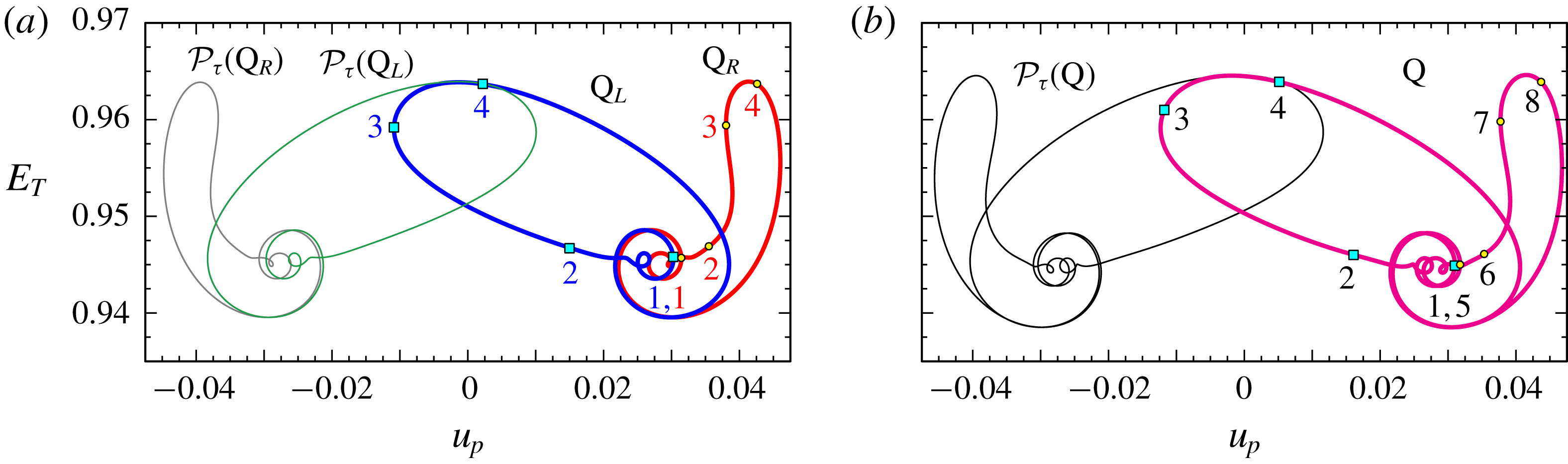
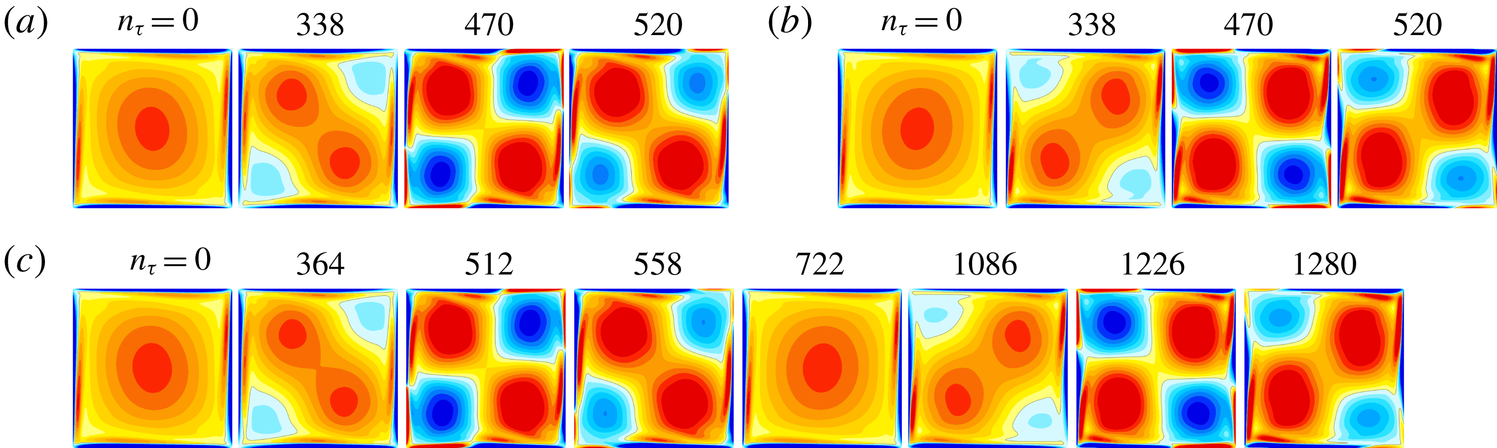
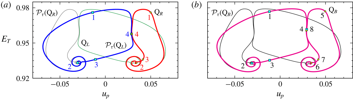
Figures 19 and 20 illustrate the dynamics just before and after the gluing bifurcation at
 $\unicode[STIX]{x1D6FC}=\unicode[STIX]{x1D6FC}_{G1}$
. At
 $\unicode[STIX]{x1D6FC}=0.125$
, the strobe map of Q
 $_{L}$
shows a slow–fast trajectory composed of saddle-focus behaviour with the slow behaviour being at the focus, followed by a rapid excursion out from the focus. The snapshots in figure 20 show the focus to be L
 $_{1:1}$
, and the trajectory away from the focus resembles L
 $_{L}$
, then L
 $_{2:2}$
briefly as it loops back, again resembling L
 $_{L}$
, and spirals in toward the focus again. The numbers labelled on the various strobe maps in figure 19 corresponds to the snapshots in figure 20. For Q
 $_{R}$
, there is also a spiral into L
 $_{1:1}$
, but the ejection out is via L
 $_{R}$
and the L
 $_{2:2}$
-like part of the trajectory at the top of the loop has more of a ‘right-hand’ bias than the L
 $_{2:2}$
-like part in Q
 $_{L}$
. After the gluing, the result is Q which consists of alternating Q
 $_{L}$
and Q
 $_{R}$
loops, as illustrated in figure 20(c) at
 $\unicode[STIX]{x1D6FC}=0.126$
. Supplementary movie 6 animates the strobes of Q
 $_{L}$
, Q
 $_{R}$
and Q shown in the figures over several hundred forcing periods, mapping out the near-homoclinic cycles involved in the gluing. Everything just described for Q
 $_{L}$
, Q
 $_{R}$
and Q also takes place for
 ${\mathcal{P}}_{\unicode[STIX]{x1D70F}}(\text{Q}_{L})$
,
 ${\mathcal{P}}_{\unicode[STIX]{x1D70F}}(\text{Q}_{R})$
and
 ${\mathcal{P}}_{\unicode[STIX]{x1D70F}}(\text{Q})$
, as illustrated by the thin curves in figure 19.
Q unglues at
 $\unicode[STIX]{x1D6FC}=\unicode[STIX]{x1D6FC}_{G2}\approx 0.135994$
. This ungluing is essentially like the first gluing at
 $\unicode[STIX]{x1D6FC}=\unicode[STIX]{x1D6FC}_{G1}$
in reverse as
 $\unicode[STIX]{x1D6FC}$
is increased. The essential difference between the first and second gluings is that the flows traverse a larger part of phase space at the larger
 $\unicode[STIX]{x1D6FC}$
. In both the first and second gluing bifurcations, for
 $\unicode[STIX]{x1D6FC}$
close to
 $\unicode[STIX]{x1D6FC}_{G1}$
and
 $\unicode[STIX]{x1D6FC}_{G2}$
, the period
 $1/f_{2}$
becomes unbounded smoothly and monotonically.
Strobe maps (every two forcing periods at forcing phase
 $\unicode[STIX]{x03C0}$
) for (a) Q
 $_{L}$
and Q
 $_{R}$
(thick blue and red curves) as well as
 ${\mathcal{P}}_{\unicode[STIX]{x1D70F}}(\text{Q}_{L})$
and
 ${\mathcal{P}}_{\unicode[STIX]{x1D70F}}(\text{Q}_{R})$
(thin green and grey curves) at
 $\unicode[STIX]{x1D6FC}=0.125$
, before the gluing bifurcation, and (b) Q (thick magenta curve) and
 ${\mathcal{P}}_{\unicode[STIX]{x1D70F}}(\text{Q})$
(thin black curve) at
 $\unicode[STIX]{x1D6FC}=0.126$
, after the gluing of Q
 $_{L}$
and Q
 $_{R}$
(and
 ${\mathcal{P}}_{\unicode[STIX]{x1D70F}}(\text{Q}_{L})$
and
 ${\mathcal{P}}_{\unicode[STIX]{x1D70F}}(\text{Q}_{R})$
). The simulations were restricted to the
 ${\mathcal{R}}_{\unicode[STIX]{x03C0}}$
symmetric subspace.

Snapshots of the vorticity at forcing phase
 $\unicode[STIX]{x03C0}$
with
 $\unicode[STIX]{x1D714}=1.41$
at the markers indicated in figure 19 (the relative times of the markers are indicated in terms of forcing periods): (a,b) Q
 $_{L}$
and Q
 $_{R}$
at
 $\unicode[STIX]{x1D6FC}=0.125$
and (c) Q at
 $\unicode[STIX]{x1D6FC}=0.126$
. Supplementary movie 6 animates the strobe maps and vorticity of the Q
 $_{L}$
, Q
 $_{R}$
and Q states at the respective parameters.

Strobe maps (every two forcing periods at forcing phase
 $\unicode[STIX]{x03C0}$
) for (a) Q
 $_{L}$
and Q
 $_{R}$
(thick blue and thin green curves) as well as
 ${\mathcal{P}}_{\unicode[STIX]{x1D70F}}(\text{Q}_{L})$
and
 ${\mathcal{P}}_{\unicode[STIX]{x1D70F}}(\text{Q}_{R})$
(thick blue and thin grey curves) at
 $\unicode[STIX]{x1D6FC}=0.146$
, before the gluing bifurcation, and (b) Q
 $_{B}$
(thick magenta curve) and
 ${\mathcal{P}}_{\unicode[STIX]{x1D70F}}(\text{Q}_{B})$
(thin black curve) at
 $\unicode[STIX]{x1D6FC}=0.147$
, after the gluing of Q
 $_{L}$
and Q
 $_{R}$
(and
 ${\mathcal{P}}_{\unicode[STIX]{x1D70F}}(\text{Q}_{L})$
and
 ${\mathcal{P}}_{\unicode[STIX]{x1D70F}}(\text{Q}_{R})$
). The simulations were restricted to the
 ${\mathcal{R}}_{\unicode[STIX]{x03C0}}$
symmetric subspace.

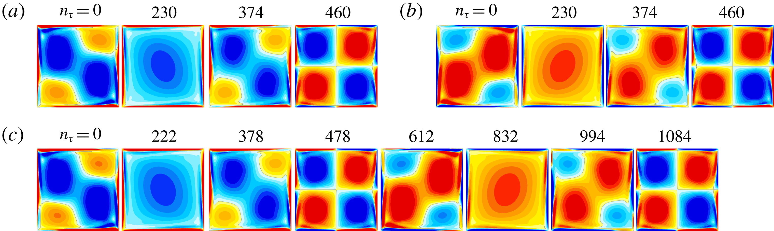
Snapshots of the vorticity at forcing phase
 $\unicode[STIX]{x03C0}$
with
 $\unicode[STIX]{x1D714}=1.41$
at the markers indicated in figure 21 (the relative times of the markers are indicated in terms of forcing periods): (a,b) Q
 $_{L}$
and Q
 $_{R}$
at
 $\unicode[STIX]{x1D6FC}=0.146$
and (c) Q
 $_{B}$
at
 $\unicode[STIX]{x1D6FC}=0.147$
. Supplementary movie 7 animates the strobe maps and vorticity of the Q
 $_{L}$
, Q
 $_{R}$
and Q
 $_{B}$
states at the respective parameters.

In figure 18(a), at
 $\unicode[STIX]{x1D6FC}_{G3}\approx 0.146631$
the period
 $1/f_{2}$
again becomes unbounded, but now this process is neither smooth nor monotonic. This gluing event is different to the two gluing bifurcations described above. The most obvious difference is that now Q
 $_{R}$
and
 ${\mathcal{P}}_{\unicode[STIX]{x1D70F}}(\text{Q}_{L})$
glue, i.e. the trajectories that glue have opposing phases at the L
 $_{1:1}$
saddle-focus. This is seen both on the strobe maps in figure 21 and in the snap shots in figure 22. There is also the conjugate gluing between Q
 $_{L}$
and
 ${\mathcal{P}}_{\unicode[STIX]{x1D70F}}(\text{Q}_{R})$
.
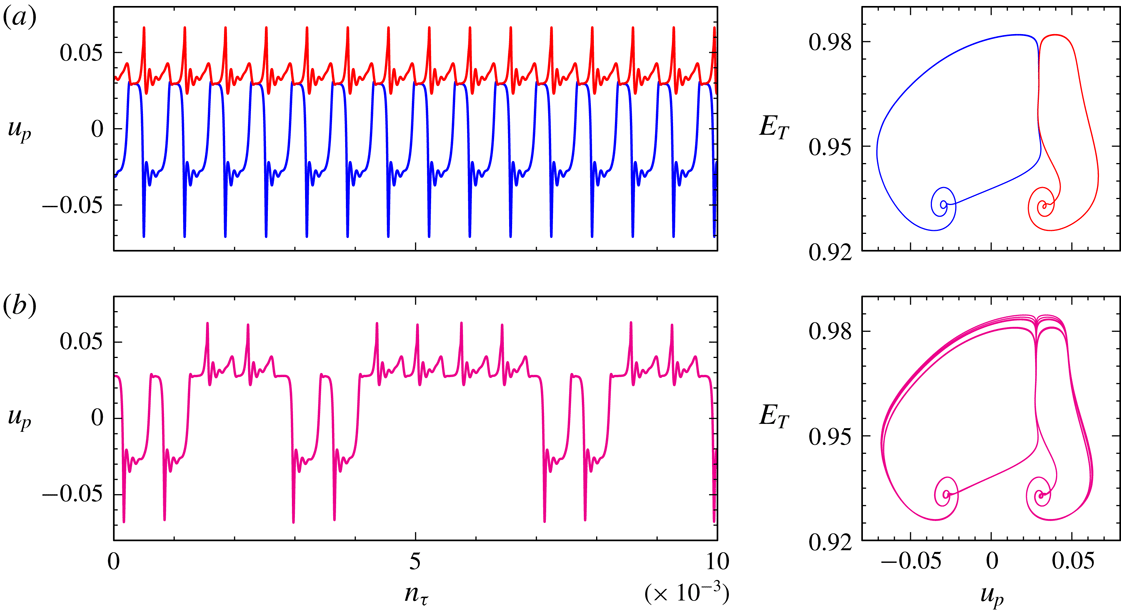
Strobed time series of the local velocity
 $u$
sampled at
 $(x_{p},z_{p})=(1/\sqrt{8},1/\sqrt{8})$
and corresponding strobe map sampled every two periods at forcing phase
 $\unicode[STIX]{x03C0}$
for (a)
 ${\mathcal{P}}_{\unicode[STIX]{x1D70F}}(\text{Q}_{L})$
and Q
 $_{R}$
(blue and red curves) at
 $\unicode[STIX]{x1D6FC}=0.14663$
before the gluing bifurcation, and (b) Q
 $_{B}$
(magenta curve) at
 $\unicode[STIX]{x1D6FC}=0.14664$
, post gluing bifurcation. The simulations were restricted to the
 ${\mathcal{R}}_{\unicode[STIX]{x03C0}}$
symmetric subspace, and only the last 10 000 forcing periods are shown of simulations with 200 000 forcing periods.

The trajectories at this third gluing are not homoclinic to L
 $_{1:1}$
(although they do get very close to L
 $_{1:1}$
and
 ${\mathcal{P}}_{\unicode[STIX]{x1D70F}}(\text{L}_{1:1})$
). Instead, as the trajectories are ejected away from the saddle foci L
 $_{1:1}$
and
 ${\mathcal{P}}_{\unicode[STIX]{x1D70F}}(\text{L}_{1:1})$
they approach the stable manifold of the saddle L
 $_{2:2}$
and become homoclinic to it at
 $\unicode[STIX]{x1D6FC}_{G3}\approx 0.146631$
. For
 $\unicode[STIX]{x1D6FC}\gtrsim \unicode[STIX]{x1D6FC}_{G3}$
, the glued trajectory Q
 $_{B}$
spirals around L
 $_{1:1}$
and
 ${\mathcal{P}}_{\unicode[STIX]{x1D70F}}(\text{L}_{1:1})$
, but spends a long time near L
 $_{2:2}$
(near points labelled 4 and 8 in figure 21
b). This suggests the existence of heteroclinic connections between the unstable manifolds of L
 $_{1:1}$
and
 ${\mathcal{P}}_{\unicode[STIX]{x1D70F}}(\text{L}_{1:1})$
and the stable manifold of L
 $_{2:2}$
, but this connection is structurally unstable and instead of coinciding, the stable and unstable manifolds intersect transversely (much like that shown in the schematic in figure 7). This implies the existence of a horse-shoe map and chaos (Smale Reference Smale1967). Indeed, we have found such chaotic dynamics for
 $\unicode[STIX]{x1D6FC}$
very close to
 $\unicode[STIX]{x1D6FC}_{G3}$
, primarily manifesting itself as trajectories with irregular numbers of orbits around L
 $_{1:1}$
and
 ${\mathcal{P}}_{\unicode[STIX]{x1D70F}}(\text{L}_{1:1})$
. Figure 23(a) shows a strobed time series of
 $u_{p}=u(1/\sqrt{8},1/\sqrt{8},t)$
at
 $\unicode[STIX]{x1D6FC}=0.14663$
and
 $\unicode[STIX]{x1D6FC}=0.14664$
, either side of the gluing at
 $\unicode[STIX]{x1D6FC}=\unicode[STIX]{x1D6FC}_{G3}$
. For the lower
 $\unicode[STIX]{x1D6FC}$
case, the responses are very regular Q
 $_{L}$
and Q
 $_{R}$
states, where as for
 $\unicode[STIX]{x1D6FC}$
slightly beyond the gluing, the Q
 $_{B}$
response shows an irregular number of left and right loops, and the accompanying strobe map in panel (b) demonstrates that the loops are also variable especially as they are ejected along the unstable manifolds of L
 $_{2:2}$
.
As
 $\unicode[STIX]{x1D6FC}$
is increased beyond
 $\unicode[STIX]{x1D6FC}_{G3}$
, the trajectory is farther away from the heteroclinic tangle, and instead follows a smooth path where it executes a single loop around L
 $_{1:1}$
followed by a single loop around
 ${\mathcal{P}}_{\unicode[STIX]{x1D70F}}(\text{L}_{1:1})$
; such a trajectory is illustrated in figure 21(b) for
 $\unicode[STIX]{x1D6FC}=0.147$
. Supplementary movie 7 animates Q
 $_{R}$
and
 ${\mathcal{P}}_{\unicode[STIX]{x1D70F}}(\text{Q}_{L})$
at
 $\unicode[STIX]{x1D6FC}=0.146$
and Q
 $_{B}$
at
 $\unicode[STIX]{x1D6FC}=0.147$
.
Supplementary movie 5 summarizes the dynamics in the
 ${\mathcal{R}}_{\unicode[STIX]{x03C0}}$
subspace at
 $\unicode[STIX]{x1D714}=1.41$
. It animates the strobe maps in steps of
 $0.01$
in
 $\unicode[STIX]{x1D6FC}$
over the
 $\unicode[STIX]{x1D6FC}$
range in figure 18.
7.3 Dynamics in the full space
We now return to the dynamics in the full space. L
 $_{L}$
and L
 $_{R}$
lose stability at
 $\unicode[STIX]{x1D6FC}\approx 0.11$
via a Neimark–Sacker bifurcation which breaks the pointwise
 ${\mathcal{R}}_{\unicode[STIX]{x03C0}}$
symmetry (in comparison, L
 $_{L}$
and L
 $_{R}$
lost stability in the
 ${\mathcal{R}}_{\unicode[STIX]{x03C0}}$
subspace at
 $\unicode[STIX]{x1D6FC}\approx 0.1208$
). This Neimark–Sacker bifurcation is designated NS
 $_{a}$
. A pair of
 ${\mathcal{G}}$
related 2-tori, T
 $_{2L}$
and T
 $_{2R}$
, are spawned, which are setwise
 ${\mathcal{R}}_{\unicode[STIX]{x03C0}}$
invariant. They inherit the subharmonic frequency
 $\unicode[STIX]{x1D714}/2$
and gain a new frequency corresponding to between six and seven forcing periods (in contrast, the 2-tori Q
 $_{L}$
and Q
 $_{R}$
that were spawned at NS
 $_{s}$
in the
 ${\mathcal{R}}_{\unicode[STIX]{x03C0}}$
subspace have a second frequency which is two orders of magnitude smaller). This new frequency corresponds to small oscillations in the degree to which the
 ${\mathcal{R}}_{\unicode[STIX]{x03C0}}$
symmetry is broken. The
 ${\mathcal{R}}_{\unicode[STIX]{x03C0}}$
asymmetry is quantified by
 $$\begin{eqnarray}A_{\unicode[STIX]{x03C0}}({\mathcal{S}})=\Vert T_{{\mathcal{R}}_{\unicode[STIX]{x03C0}}({\mathcal{S}})}-T_{{\mathcal{S}}}\Vert /\Vert T_{{\mathcal{S}}}\Vert ,\end{eqnarray}$$
where
 ${\mathcal{S}}$
is the state,
 $T_{{\mathcal{S}}}$
is its temperature, and
 ${\mathcal{R}}_{\unicode[STIX]{x03C0}}({\mathcal{S}})$
is the result of the action of
 ${\mathcal{R}}_{\unicode[STIX]{x03C0}}$
on
 ${\mathcal{S}}$
. For T
 $_{2L}$
and T
 $_{2R}$
,
 $A_{\unicode[STIX]{x03C0}}\sim 10^{-3}$
; in essence they are weakly modulated L
 $_{L}$
and L
 $_{R}$
.
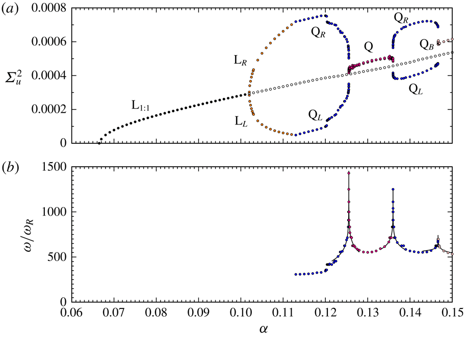
Variance of the horizontal velocity
 $\unicode[STIX]{x1D6F4}_{u}^{2}$
at the point
 $(x_{p},z_{p})=(1/\sqrt{8},1/\sqrt{8})$
for
 $\unicode[STIX]{x1D714}=1.41$
for various observed states, as indicated. In panel (a), the L
 $_{1:1}$
is unstable for
 $\unicode[STIX]{x1D6FC}>0.102$
and is obtained through a transient. Supplementary movie 8 animates the strobe maps of the states in steps of 0.01 in
 $\unicode[STIX]{x1D6FC}$
.

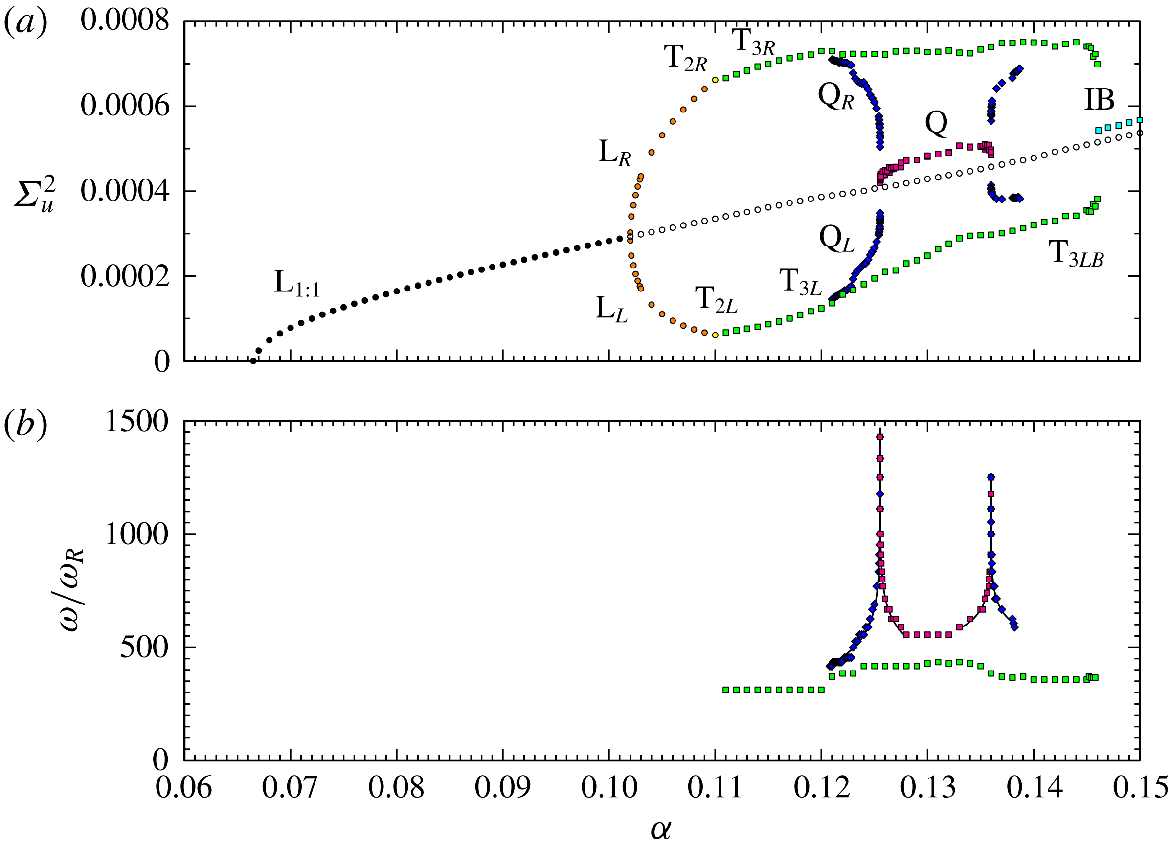
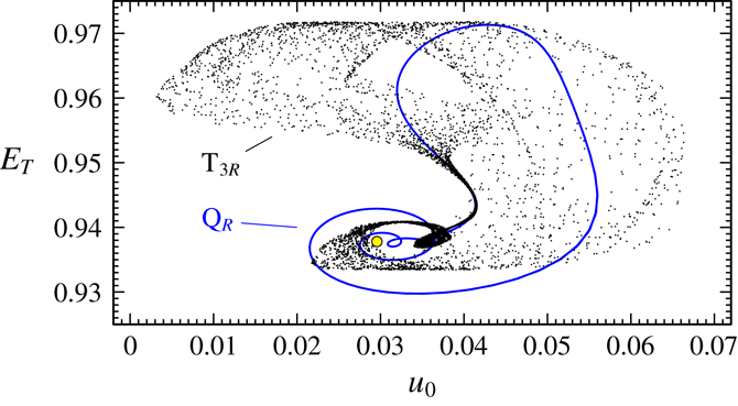
Figure 24 shows the velocity variances of the states involved in the full space as
 $\unicode[STIX]{x1D6FC}$
is increased for fixed
 $\unicode[STIX]{x1D714}=1.41$
, along with the long periods of some of the quasi-periodic states. It is very similar to figure 18, which shows the corresponding measures in the
 ${\mathcal{R}}_{\unicode[STIX]{x03C0}}$
subspace. On the scale of the figure, T
 $_{2L}$
and T
 $_{2R}$
are stable only at the symbol shown (in yellow), and they lose stability with a very slight increase in
 $\unicode[STIX]{x1D6FC}$
. A pair of
 ${\mathcal{G}}$
-related 3-tori, T
 $_{3L}$
and T
 $_{3R}$
are spawned. They inherit the two frequencies from T
 $_{2L}$
and T
 $_{2R}$
, and the third new frequency is very low, approximately two orders of magnitude smaller, and corresponds to slow drifts towards and away from the
 ${\mathcal{R}}_{\unicode[STIX]{x03C0}}$
symmetric subspace. During these drifts,
 $A_{\unicode[STIX]{x03C0}}$
varies between
 $O(10^{-3}{-}10^{-4})$
and
 $O(10^{-1})$
.
At
 $\unicode[STIX]{x1D6FC}\approx 0.121$
two new stable 3-tori states are observed. They are very similar to of Q
 $_{L}$
and Q
 $_{R}$
in the
 ${\mathcal{R}}_{\unicode[STIX]{x03C0}}$
subspace, with the only essential difference being that in the full space they have a very weak drift away from and back to the
 ${\mathcal{R}}_{\unicode[STIX]{x03C0}}$
subspace. As such, we shall simply call them Q
 $_{L}$
and Q
 $_{R}$
. In contrast, T
 $_{3L}$
and T
 $_{3R}$
are never
 ${\mathcal{R}}_{\unicode[STIX]{x03C0}}$
symmetric even though they also drift toward and away from the
 ${\mathcal{R}}_{\unicode[STIX]{x03C0}}$
subspace in a regular fashion. The T
 $_{3L}$
and T
 $_{3R}$
also drift toward and away from the
 ${\mathcal{K}}_{z}$
subspace during the
 ${\mathcal{R}}_{\unicode[STIX]{x03C0}}$
subspace drifts. This
 ${\mathcal{K}}_{z}$
subspace excursion gains intensity as the forcing amplitude
 $\unicode[STIX]{x1D6FC}$
is increased, and is associated with the 2-torus S
 $_{2}$
and 3-torus S
 $_{3}$
sloshing flows identified in the
 ${\mathcal{K}}_{z}$
symmetric subspace.
Strobe maps for the flow taken every two forcing periods at forcing phase
 $\unicode[STIX]{x03C0}$
at
 $\unicode[STIX]{x1D6FC}=0.138$
for the stable Q
 $_{R}$
(blue), stable T
 $_{3R}$
(black) and unstable L
 $_{1:1}$
(yellow). See supplementary movie 9 for animated strobes of Q
 $_{R}$
and T
 $_{3R}$
.

Q
 $_{L}$
and Q
 $_{R}$
undergo the first and second gluing bifurcations with essentially no difference from what we observed earlier in the
 ${\mathcal{R}}_{\unicode[STIX]{x03C0}}$
subspace. Over the same interval in
 $\unicode[STIX]{x1D6FC}$
, T
 $_{3L}$
and T
 $_{3R}$
follow similar trajectories in phase space with two important differences. They do not become homoclinic to
 $L_{1:1}$
(although they do spiral in close to it), and they have a pronounced excursion to the sloshing S
 $_{2}$
or S
 $_{3}$
(depending on the value of
 $\unicode[STIX]{x1D6FC}$
). Q
 $_{L}$
and Q
 $_{R}$
are completely oblivious to S
 $_{2}$
and S
 $_{3}$
as S
 $_{2}$
and S
 $_{3}$
do not exist in the
 ${\mathcal{R}}_{\unicode[STIX]{x03C0}}$
subspace. Strobes of Q
 $_{R}$
and T
 $_{3R}$
are shown in supplementary movie 9 at
 $\unicode[STIX]{x1D6FC}=0.138$
; the erratic behaviour in T
 $_{3R}$
is due to the trajectory passing very close by S
 $_{3}$
. The corresponding strobe maps are shown in figure 25 with the unstable L
 $_{1:1}$
shown as a yellow marker. Q
 $_{L}$
and Q
 $_{R}$
are no longer stable for
 $\unicode[STIX]{x1D6FC}\gtrsim 0.139$
, and T
 $_{3L}$
or T
 $_{3R}$
are the only observed states until
 $\unicode[STIX]{x1D6FC}\gtrapprox 0.146$
, the flow then consists of intermittent bursts, displaying behaviour associated with the previously described states for irregular time intervals. This intermittent bursting state IB roughly coincides with the appearance of the Q
 $_{B}$
state in the
 ${\mathcal{R}}_{\unicode[STIX]{x03C0}}$
subspace.
Supplementary movie 8 summarizes the dynamics as
 $\unicode[STIX]{x1D6FC}$
is increased with
 $\unicode[STIX]{x1D714}=1.41$
in the full space. The left panel has figure 24 for reference and the
 $(u_{p},E_{T})$
strobe maps are in the right panel.
7.4 The big picture of the L
$_{1:1}$
tip

Now, we consider how the various dynamic responses in the different parameter regimes of the tip of the
 $1:1$
horn described earlier are interrelated. We have traced out both the pitchfork bifurcation and the Neimark–Sacker bifurcation NS
 $_{a}$
in
 $(\unicode[STIX]{x1D714},\unicode[STIX]{x1D6FC})$
space, and their loci are shown in figure 26. These curves appear to meet the Neimark–Sacker curve NS (described in § 6) at a point PN (green circular symbol in the figure). For
 $\unicode[STIX]{x1D714}\lesssim 1.415$
, T
 $_{2L}$
and T
 $_{2R}$
are only stable in a very thin wedge region emanating from PN (too thin to see on the scale of the figure). For
 $\unicode[STIX]{x1D714}\gtrsim 1.415$
, the Neimark–Sacker bifurcation does not break the pointwise
 ${\mathcal{R}}_{\unicode[STIX]{x03C0}}$
symmetry. The Neimark–Sacker bifurcation curve is the continuation of NS
 $_{s}$
which was identified in the
 ${\mathcal{R}}_{\unicode[STIX]{x03C0}}$
subspace (see § 7.2). It also meets the point PN (it is shown as a dashed red curve for
 $\unicode[STIX]{x1D714}\lesssim 1.415$
). The 2-tori that are spawned at NS
 $_{s}$
, Q
 $_{L}$
and Q
 $_{R}$
, are stable over a larger range in
 $\unicode[STIX]{x1D6FC}$
than those spawned at NS
 $_{a}$
. Above the NS
 $_{a}$
and NS
 $_{s}$
there are multiple stable states, some of which undergo homoclinic bifurcations. The region between these Neimark–Sacker curves and the dashed curve denoted ‘breakup’ has very complicated dynamics, some of which we describe above for
 $\unicode[STIX]{x1D714}=1.41$
(see § 7.3). In the middle of the complex region is a pair of homoclinic gluing bifurcation curves along which
 ${\mathcal{G}}$
-related states simultaneously become homoclinic to a setwise
 ${\mathcal{G}}$
invariant saddle state (the unstable L
 $_{1:1}$
). The green region of figure 26 demarcates where pointwise
 ${\mathcal{R}}_{\unicode[STIX]{x03C0}}$
symmetry is broken. In between the second gluing bifurcation curve and the breakup curve, there are multiple states manifesting slow drifts towards and away from various saddle solutions that are related not just to L
 $_{1:1}$
, but also the secondary instability of the basic state (L
 $_{2:2}$
), and various secondary instabilities of these that we have been able to identify.
Bifurcation curves in the
 $1:1$
resonance tongue.

8 Discussion and conclusions
The nonlinear responses of a stably stratified fluid in a square cavity subjected to parametric forcing consisting of vertical harmonic oscillations has been explored numerically. While linear Floquet analysis about the basic state predicts the critical forcing amplitude and frequency for the onset of instability, it does not distinguish between supercritical and subcritical onset, nor to what the instability saturates to nonlinearly. The nonlinear results are in very good agreement with the Floquet analysis in determining the instability of the basic state, in which the viscous eigenmodes of the cavity are excited via parametric resonance.
The present study is in the regime where the product of the buoyancy frequency and the viscous time scale is
 $R_{N}=2\times 10^{4}$
, in which many of the resonance tongues corresponding to the lower-order eigenmodes are clearly identified. The nonlinear responses clearly demonstrate the subcritical nature of the primary instability from the basic state on the low forcing frequency side of the resonance tongues. The dynamics near the tip of the broadest tongue, the subharmonic
 $1:1$
tongue, was explored in detail. The period-doubled limit cycle response L
 $_{1:1}$
undergoes both pitchfork and Neimark–Sacker bifurcations, resulting in symmetry conjugate limit cycles and quasi-periodic 2-tori in different parts of the tip, and the basic state also loses stability to the first harmonic viscous eigenmode L
 $_{2:2}$
. All of these states undergo secondary bifurcations, resulting in a multiplicity of unstable saddle states. We have identified three codimension-two points that organize the responses.
The first of these is a generalized flip located at the very tip of the tongue, where the instability of the basic state changes from supercritical to subcritical as the forcing frequency is reduced. The subcritical flip bifurcation leads to a fold bifurcation curve along which the unstable saddle L
 $_{1:1}$
that bifurcates from the basic state is folded back and stabilized. The stabilized upper branch L
 $_{1:1}$
becomes unstable via a Neimark–Sacker bifurcation as the forcing frequency is increased.
The Neimark–Sacker curve and the fold curve meet at a second codimension-two point that we analysed. This flow involves heteroclinic behaviour in its normal form, but the heteroclinic behaviour is not structurally stable, and the full Navier–Stokes system reveals a complex homoclinic-doubling response, which has some similarities to the dynamics of the logistic map, in the parameter region of the heteroclinics in the normal form. Beyond this region, all states locally associated with the codimension-two bifurcation are unstable, and the flow abruptly collapses to the basic state.
The third codimension-two point is near the centre of the tip where the Neimark–Sacker and the pitchfork curves meet. In the neighbourhood of this point, to the high-frequency side, the symmetry-broken limit cycles undergo Neimark–Sacker bifurcations and then the resulting conjugate 2-tori simultaneously become homoclinic to the saddle L
 $_{1:1}$
in a gluing bifurcation. The resulting glued symmetric 2-torus unglues as the forcing amplitude is increased. The two curves of gluing bifurcations also meet at the third codimension-two point. There are other complicated states in this regime, and they all involve slow drifts into and out of symmetric subspaces, and near heteroclinic collisions with the various saddle states that have been excited. As the forcing amplitude is increased, the stable and unstable manifolds involved in the heteroclinic behaviour become increasingly tangled, resulting in intermittently bursting flows.
Despite the details the
 $1:1$
resonance tongue obtained in this study, the details of the other resonance tongues remain unresolved. It is likely that the dynamics observed near the generalized flip and fold-Neimark–Sacker codimension-two points will be common to the other tongues, but the symmetry breaking and restoring events will necessarily differ as the primary viscous eigenmodes associated with other tongues have symmetries that differ from those of L
 $_{1:1}$
.
Much of the dynamics we have found is consistent with the experimental observations of Benielli & Sommeria (Reference Benielli and Sommeria1998), whose focus on the 1:1 resonance tongue motivated our study, even though there are obvious differences between their experimental set-up and our numerical model. They used salt as their stratifying agent, whereas we use temperature. Apart from having a two order of magnitude difference in the Prandtl/Schmidt number, the boundary condition on the horizontal end walls are different. These differences seem to be of secondary importance. Our simulations are two-dimensional, but the experiments are necessarily three-dimensional. However, the spanwise dimension of their cavity was considerably less than the other two dimensions, and in the central tip region they were able to parametrically excite the two-dimensional mode (L
 $_{1:1}$
), and observed some of the dynamics we report on, albeit at higher
 $R_{N}$
compared to
 $R_{N}=2\times 10^{4}$
used here (presumably to overcome the viscous damping from the spanwise walls). They observed various
 $m:n$
modes, and heteroclinic drifts between some these, akin to the heteroclinic intermittency (IB) we reported from the
 ${\mathcal{R}}_{\unicode[STIX]{x03C0}}$
subspace simulations. They also observed localized small-scale three-dimensional flows associated with wave breaking events at larger forcing amplitudes. We have observed two-dimensional wave breaking in some regimes (Yalim et al.
Reference Yalim, Welfert, Lopez and Wu2017a
; Yalim, Welfert, Lopez & Wu Reference Yalim, Welfert, Lopez and Wu2017b
), but these events were short lived. The breaking produces small-scale intense vortices, but these are quickly dissipated. The present study, being restricted to two-dimensional flow, lacks the vortex tilting and stretching mechanism that would allow for intensification of the strength of the small length scales on a time scale that is faster than that in which the viscous dissipation acts on. Studies in the wave breaking regime for three-dimensional flows are currently under investigation in a short spanwise container, similar to the experimental configuration of Benielli & Sommeria (Reference Benielli and Sommeria1998). Some of the two-dimensional dynamics reported here has been qualitatively reproduced, in particular the gluing bifurcations involving L
 $_{1:1}$
, L
 $_{L}$
, L
 $_{R}$
and L
 $_{2:2}$
. Details will be reported on subsequently.
Acknowledgements
We thank ASU Research Computing facilities and the NSF XSEDE program for providing computing resources, K. Wu for the original solver codebase and Professor F. Marques for his expertise.
Supplementary movies
Supplementary movies are available at https://doi.org/10.1017/jfm.2019.347.