






1. Introduction
Plates with orifices are very common elements adopted in numerous industrial applications, like, for example, silencers, fuel injectors or wind instruments. Under the effect of a harmonic incident acoustic wave, the vortex sheet formed at the lip of the aperture becomes periodically modulated and acts as an amplifier due to a Kelvin–Helmholtz instability, reorganising the jet into an arrangement of vortex rings. The generation of vorticity is an efficient mechanism to dissipate acoustic energy, as a consequence, the use of multiple perforated plates traversed by a mean flow is widely employed as a sound attenuator device for industrial applications, such as gas turbine combustion systems. These systems may suffer from thermoacoustic instabilities because of the potential for unsteady heat release, which can damage the combustion system itself. The flow through a perforated liner with bias flow has been studied experimentally by Heuwinkel, Enghardt & Rohle (Reference Heuwinkel, Enghardt and Rohle2007) while Hughes & Dowling (Reference Hughes and Dowling1990), Eldredge & Dowling (Reference Eldredge and Dowling2003) and Rupp, Carrotte & Macquisten (Reference Rupp, Carrotte and Macquisten2012) have conducted both experimental and theoretical investigations. There are, however, situations where the flow through a hole can lead to the opposite effect, namely spontaneous self-oscillations and sound emissions. A particularly favourable situation with respect to sound emission is the flow through two successive holes, as encountered, for instance, in bird calls and tea kettle whistles (Henrywood & Agarwal Reference Henrywood and Agarwal2013; Longobardi et al. Reference Longobardi, Fabre, Bonnefis, Citro, Giannetti and Luchini2021). Although less common, the flow through a single hole can also lead to powerful sound emissions. As in other related examples of aeroacoustic resonators, (including, for instance, the ‘edge tone’ encountered in the mouthpiece of a recorder or organ pipe), two situations may occur. In the first one, the frequency of the whistling may be directly selected by that of an acoustic resonator located in the vicinity of the hole. This is, for instance, the case for the so-called ‘pipe tone’ (or pfeifenton), corresponding to a long cylindrical pipe terminated by an aperture of smaller section. In this configuration, which was intensively investigated experimentally by Anderson (Reference Anderson1954), the frequency of the whistling directly corresponds to one of the resonance frequencies of the pipe. In the second one, the frequency may be selected by the flow itself regardless of the existence of any acoustic resonator. This situation was noted by Bouasse (Reference Bouasse1929), who observed that the flow through a hole in a thick plate separating two large chambers leads to a whistling with a frequency proportional to the thickness of the hole. This observation was rediscovered by Jing & Sun (Reference Jing and Sun2000) and Su et al. (Reference Su, Rupp, Garmory and Carrotte2015) who, in an effort to improve the performance of perforated plates as sound dampers, reported that, in some circumstances, these devices could lead to self-sustained whistling. In music acoustics one observes the interaction between the two type of mechanisms, cf. Coltman (Reference Coltman1976). In the case of the flue instrument, the so-called edge-tone oscillation can coexist with the pipe tone and under some specific circumstances, as, for example, during the attack transients, it may be dominant, cf. Castellengo (Reference Castellengo1999). Verge, Hirschberg & Causse (Reference Verge, Hirschberg and Causse1997) proposed a lumped model for flue instruments where these two feedback loops can coexist and interfere: a hydrodynamic loop responsible for the edge tone and a cavity loop responsible for the pipe tone. On the contrary, in the case of the flow past an aperture both mechanisms are associated with the same feedback loop, which is modified by placing a cavity upstream of the perforation. These two situations respectively correspond to the so-called class III and class II categories of aeroacoustic resonators, following the classification of Chanaud (Reference Chanaud1970).
Recently, Fabre et al. (Reference Fabre, Longobardi, Bonnefis and Luchini2019) used the linearized Navier–Stokes equations (LNSE) approach to investigate the unsteady flow through a circular aperture in a thin plate subjected to harmonic forcing. A novel non-reflecting boundary condition called the complex mapping method (Sierra, Fabre & Citro Reference Sierra, Fabre and Citro2020) was introduced to overcome the numerical difficulties created by the strong spatial amplification of the fluctuations. The approach allows computing in a rigorous way the impedance of the hole, namely the ratio between unsteady pressure difference across the orifice and unsteady volume flow rate through the orifice, a quantity which can be directly introduced in more elaborate acoustical models. In that study, the authors confirmed that the LNSE can be effectively adopted to predict the impedance even in cases where the spatial evolution of the perturbations is rapidly dominated by nonlinear effects. The same approach was subsequently used by Fabre et al. (Reference Fabre, Longobardi, Citro and Luchini2020) for the case of a hole through a thick plate. An important result is that, for sufficiently thick holes, the impedance can acquire a negative real part in some ranges of forcing frequencies, indicating that energy can be extracted from the flow, thus providing a source for self-oscillations. Investigation of the structural sensitivity also allowed the authors to demonstrate that the hydrodynamic instability of the shear layer separating the jet from the recirculation bubble is the driving motor for the observed phenomenon. This corresponds to the same instability as in the jet of a flue instrument or the shear layer for a grazing flow along a cavity, cf. Dai & Aurégan (Reference Dai and Aurégan2016, Reference Dai and Aurégan2018). In this flow configuration, the sharpness of the aperture corner creates a recirculation bubble that enhances the instability mechanism.
The response of a system to a harmonic forcing is naturally studied via a transfer function: here it corresponds to the concept of impedance, which can also be used to obtain important information regarding the stability properties of a system. First, plotting the impedance in the form of Nyquist diagrams (namely a parametric representation of  $Z(\omega )$ in the complex plane for real values of
 $\omega$) provides a direct way to determine the number of unstable modes of the system, as a function of the number of times the Nyquist contour encircles the origin. Secondly, when the system has a complex eigenvalue located close to the real
 $\omega$-axis, an approximation of the eigenvalue can be obtained from a Taylor expansion of the impedance function around the real axis. Such methods are widely used in several fields such as in automatics or electronics, but remain underemployed in the flow instability community where eigenvalue computation remains the preferred approach. Note, however, that the second idea was recently applied successfully by Ferreira Sabino et al. (Reference Ferreira Sabino, Fabre, Leontini and Lo Jacono2020) for the problem of vortex-induced vibrations for a spring-mounted cylinder.
The links between impedance and stability properties were explored by Fabre et al. (Reference Fabre, Longobardi, Citro and Luchini2020) for the jet flow through a hole. The discussion revealed the existence of two different instability mechanisms leading to sound production: a purely hydrodynamic instability characterised by spontaneous self-oscillations existing in the absence of any incoming acoustic wave, and a conditional instability due to an over-reflection of acoustic waves. Simple criteria formulated in terms of the impedance were given for both kinds of instabilities, allowing us to determine their range of existences as a function of the hole aspect ratio and the Reynolds number. Among the studies considering a multiply perforated plate, Jing & Sun (Reference Jing and Sun2000) and Su et al. (Reference Su, Rupp, Garmory and Carrotte2015) measured experimentally the impedances for several configurations with variable hole thickness parameter values, which are in good accordance with the first branch of conditional unstable modes, cf. Fabre et al. (Reference Fabre, Longobardi, Citro and Luchini2020, § 8). Moussou et al. (Reference Moussou, Testud, Auregan and Hirschberg2007) studied experimentally a long pipe with a constriction for a number of values of the constriction ratio and the thickness ratio. In this study, they identified both the first and second branch of conditionally unstable modes.
In the approach of Fabre et al. (Reference Fabre, Longobardi, Citro and Luchini2020), the flow was assumed as locally incompressible, a hypothesis which is expected to be valid for small values of the square of the Helmholtz number ( $He^{2} = \omega ^{2} M^{2}$), and which does not directly allow predicting the acoustic field. Nevertheless, they suggested that the locally incompressible solution could be matched to outer solutions incorporating compressibility effects, leading to more elaborate models applicable in situations incorporating, for instance, acoustic resonators and radiation in an open domain.
The object of the present paper is precisely to show how the impedance computations of Fabre et al. (Reference Fabre, Longobardi, Citro and Luchini2020) based on a locally incompressible solution can be used to build a model applicable for a realistic situation involving compressibility. In addition, acoustic pressure fields, obtained from full compressible LNSE computations complement the study. Two generic situations are considered. In the first situation referred to as cavity/open configuration, the domain located upstream of the hole is considered as a closed cavity of finite volume, while the downstream domain is considered as open. We then show that the presence of the upstream resonator can effectively lead to instabilities, as predicted by the conditional instability criterion. The second situation, referred to as open/open configuration, corresponds to the case where the two regions, upstream and downstream of the hole, are considered as open domains of large dimension. We show, in this case, that an instability of purely a hydrodynamic type can arise.
The paper is organized as follows. In § 2 the two generic situations are introduced, and the parameters are outlined. In § 3 we introduce an asymptotically matched or lumped model which allows defining a global impedance for the selected configuration by combining the hole impedance as computed by Fabre et al. (Reference Fabre, Longobardi, Citro and Luchini2020) and the impedances of the upstream and downstream domains. We also show that a Taylor expansion of this impedance around the real  $\omega$-axis can be used to obtain an instability criterion and an estimation of the eigenvalue of the unstable modes in the fully compressible case. In § 4 we introduce a numerical resolution method for the eigenvalue problem in a fully compressible set-up. In § 5 we present results for the cavity/open configuration. We compare both approaches, demonstrating that the asymptotic model is effectively accurate for low Mach numbers. We then provide a parametric study for both problems, thanks to the asymptotic model. Section 6 presents results for the open/open configuration. We particularly investigate the effect of compressibility on the purely hydrodynamic instability mechanism identified by Fabre et al. (Reference Fabre, Longobardi, Citro and Luchini2020), and also consider the acoustic directivity of far-field sound emission.
2. Problem definition
2.1. Fluid parameters
The fluid is considered as a perfect gas with specific constant  $R_g$ and adiabatic index
 $\gamma = 1.4$. We denote with
 $\rho _0$ the reference density and with
 $T_0$ the reference temperature (both corresponding to the values in the upstream domain). The fluid is assumed to have constant dynamic viscosity
 $\mu$ and heat conductivity
 $\alpha$. The mass flow rate at the inlet of the domain is denoted with
 $\dot m_0$, while the mean velocity across the hole is
 $U_M = \dot m_0 / (\rho _0 {\rm \pi}R_h^{2})$. Based on this velocity scale and the hole diameter
 $D_h = 2 R_h$, the Reynolds and Mach numbers of the flow are then defined as
 \begin{equation} {\textit{Re}}= \frac{\rho_0 D_h U_M}{\mu} \equiv \frac{2 \dot m_0 }{{\rm \pi} R_{h} \mu};\quad M = \frac{U_M}{c_0}\quad \mbox{with } c_0 = \sqrt{\gamma R_g T_0}. \end{equation}
The fluid is also characterised by a Prandtl number  $Pr= \rho _0 \alpha / \mu$ which is here assumed to be
 $Pr =0.7$.
2.2. Open/open configuration
In the first configuration, termed open/open configuration and sketched in figure 1, we consider that a plate separates two semi-infinite ‘open domains’ of large dimensions. By ‘open domain’ we mean that acoustic waves generated at either side of the hole propagate towards infinity without reflection. Denoting with  $L_h$ the thickness of the plate, the geometry is thus completely defined by a single dimensionless parameter, the aspect ratio of the hole, defined as
 \begin{equation} \beta = \frac{L_h}{2R_h} = \frac{L_h}{D_h}. \end{equation}
In the fully compressible simulations, boundary conditions have to be applied at the boundary of the domain. For simplicity, a half-spherical boundary is considered upstream, and a uniform radial velocity is imposed, as sketched in the figure. Non-reflective boundary conditions used for the compressible computations are introduced and explained in details in § 4.
Sketch of the open/open configuration.

2.3. Cavity/open configuration
The second considered configuration, termed cavity/open configuration, is sketched in figure 2. This configuration is selected here to study, in the simplest possible setting, the coupling of the hole with a cavity acting as a resonator. The upper domain is considered as a cavity of dimensions  $L_{in}, R_{in}$ which acts as a Helmholtz resonator. Therefore, only its volume is relevant, not the exact dimensions
 $L_{in}, R_{in}$ or the particular geometry. Thus, in addition to the aspect ratio
 $\beta$ defined above, a second geometrical parameter enters the problem, namely the dimensionless volume defined as
 \begin{equation} V_{in} = \frac{L_{in} {\rm \pi}R_{in}^{2}}{R_h^{3}}. \end{equation}
The inlet condition is imposed at the leftmost boundary where, for simplicity, a constant velocity profile is enforced, as sketched in the figure.
Sketch of the cavity/open configuration.

3. Matched asymptotic model
Before considering the resolution of the problem in a fully compressible setting, we detail here a matched asymptotic model which allows us to compute a total impedance characterising the behaviour of linear perturbations of the full system. We first explain how the different regions of the flow domain can be described to obtain the model, and then discuss how the derived total impedance can be used to predict the onset of instabilities.
3.1. Matching principle
Under the hypothesis that the Mach number is small and that acoustic wavelengths are much larger than the dimensions of the hole (acoustic compactness hypothesis), it is possible to assume that the flow in the vicinity of the hole is locally incompressible, while compressibility is only relevant in the upstream and downstream domains. This hypothesis is at the origin of the asymptotically matched or lumped model. The ingredients required for matching are the pressure  $p_{in}(t)$ just upstream of the hole, the pressure
 $p_{out}(t)$ just downstream of the hole, and the volume flow rate
 $q(t)$ across the hole. Working in the frequency domain, all these quantities are expanded as a constant value associated with the base flow, plus a perturbation with harmonic dependency
 ${\rm e}^{-{\rm i}\tilde {\omega } t}$, where
 $\tilde {\omega }$ is a (possibly complex) dimensional frequency,
 \begin{equation} \left.\begin{gathered} p_{in}(t) = P_{in} + p'_{in}\,{\rm e}^{-{\rm i}\tilde{\omega} t},\quad p_{out}(t) = P_{out} + p'_{out}\,{\rm e}^{-{\rm i}{\tilde{\omega}} t,} \\ q(t) = Q_0 +q'\,{\rm e}^{-{\rm i}{\tilde{\omega}} t,}. \end{gathered}\right\} \end{equation}
It is important to understand that here  $p'_{out}$ corresponds to the level of the fluctuating pressure field at distances
 $\| \boldsymbol {x} \|$ considered large in relation to the hole dimension but small compared with the acoustic wavelength, i.e.
 $R_h \ll \| \boldsymbol {x} \| \ll \tilde {\lambda }$, with
 $\tilde {\lambda } = 2{\rm \pi} c_0/\tilde {\omega }$. Consequently, this pressure level corresponds both to the outer limit for the inner solution, and to the inner limit for the outer solution of the classic matched asymptotic expansion procedure. The same holds for
 $p'_{in}$ which is also used as a matching limit between inner and outer solutions.
3.2. Impedance modelling
3.2.1. Inner region: hole impedance
The inner region, located in the vicinity of the hole (delimited by dotted lines in figures 1 and 2), is governed by the incompressible LNSE. A resolution method for this problem was introduced and validated in Fabre et al. (Reference Fabre, Longobardi, Citro and Luchini2020): for the benefit of the reader, this approach is also briefly summarised in § A. The cited method allows us ultimately to deduce the (dimensionless) hole impedance  $Z_h(\omega )$ defined as
 \begin{equation} Z_h(\omega) = \left[ \frac{R_h^{2}}{\rho_0 U_M} \right] \frac{p'_{in}-p'_{out}}{q'}. \end{equation}
Here the factor  $R_h^{2}/(\rho _0 U_M)$ is introduced to turn the impedance into a dimensionless one, since the dimensional impedance
 $(p'_{in}-p'_{out})/q'$ has physical units
 $\textrm {kg}\,\textrm {s}^{-1}\,\textrm {m}^{-4}$ in the international system, and it is a function of the dimensionless frequency
 $\omega =R_h \tilde {\omega } / U_M$.
The impedance is ultimately searched as  $Z_h = {{{\boldsymbol{P}}}} \cdot {({\boldsymbol{\mathsf{LNS}}} + \textrm {i}\omega {\boldsymbol{\mathsf{B}}} )}^{-1} \cdot \boldsymbol{F}$, where
 $\boldsymbol{F}$ represents a forcing of the LNSE by an imposed flow rate,
 ${( {\boldsymbol{\mathsf{LNS}}} + \textrm {i}\omega {\boldsymbol{\mathsf{B}}} )}^{-1}$ is the linear resolvent of the incompressible LNSE, and
 $\boldsymbol{P}$ is an operator allowing us to extract the overall pressure jump from the linear perturbation. After a convenient discretization, computation of the impedance is thus straightforward and only requires inversion of a single linear problem. More details are given in Appendix A. It is thus much faster in comparison to eigenvalue computation, which, using the shift-and-invert method, typically requires numerous iterative resolutions of such problems. Once
 $Z_h(\omega )$ is computed and tabulated (Fabre et al. Reference Fabre, Longobardi, Citro and Luchini2020) a complete parametric study in terms of Mach number and the cavity volume can be performed as shown below.
3.2.2. Downstream region: radiation impedance
When observed from a large distance, the hole can be seen as a monopolar source, which classically gives rise to spherical diverging waves. This is classically described by a radiation impedance defined as the ratio between pressure  $p'_{out}$ and flow rate
 $q'$. This impedance can be obtained by asymptotically matching an acoustically compact inner solution with a monopolar acoustic source, cf. Fletcher & Rossing (Reference Fletcher and Rossing2012), Pierce (Reference Pierce2019) and Rossing (Reference Rossing2007). The computation is also reproduced in Fabre et al. (Reference Fabre, Longobardi, Citro and Luchini2020, Appendix A therein). When expressed in dimensionless variables, the result is a purely real impedance
 $Z_{rad}$ given by
 \begin{equation} Z_{rad} = \left[ \frac{R_h^{2}}{\rho_0 U_M} \right]\frac{p'_{out}}{q'} = \frac{M \omega^{2}}{2 {\rm \pi}}. \end{equation}
3.2.3. Upstream region: case of an open domain
In a similar way, in the case of the ‘open domain’ (figure 1), one can introduce the impedance of the inlet domain  $Z_{in}$, which is defined as
 \begin{equation} Z_{in} = \left[\frac{R_h^{2}}{\rho_0 U_M} \right]\frac{p'_{in}}{q'} ={-} \frac{M \omega^{2}}{2 {\rm \pi}} ={-} Z_{rad}. \end{equation}
3.2.4. Upstream region: case of a cavity
In the case where the upstream domain is considered as a closed cavity (figure 2), we assume that this cavity acts as a Helmholtz resonator, namely the pressure  $p' = p'_{in}$, and the density
 $\rho ' = \rho '_{in}$ are uniform. Then a mass budget leads to
 \begin{equation} V_{in} c_0^{2} \frac{{{\rm d}} \rho_{in}'}{{{\rm d}}t} = V_{in} \frac{{{\rm d}}p'_{in}}{{{\rm d}}t} = \rho_0 q', \end{equation}
which allows the introduction of the impedance of the cavity  $Z_{cav}$,
 \begin{equation} Z_{cav} = \left[\frac{R_h^{2}}{\rho_0 U_M} \right]\frac{p'_{in}}{q'} = \frac{i}{ \omega M^{2} V_{in}} = \frac{i}{ \omega \chi },\quad \chi = M^{2} V_{in}. \end{equation}
Note that this expression indicates that the cavity acts as a capacitor for an electrical circuit or as a spring in a mechanical system. Moreover, its characteristics only depend upon the quantity  $\chi = M^{2} V_{in}$ which combines the Mach number and the dimensionless volume of the cavity. Such a model could be complemented with the addition of two other terms that have been neglected. In particular, one could include on the left-hand side of the mass balance the deviation from isentropic pressure fluctuations due to, for instance, the effects of the thermal boundary layer and on the right-hand side, the convective term involving density fluctuations. These terms have been neglected based on the fact that velocity and temperature gradients within the cavity are small as long as the ratio between the height of the cavity and the radius of the hole is large. In our study, this corresponds to
 $L_{in} = R_{in} = (V_{in}/{\rm \pi} )^{1/3} \gg R_{h}$, which holds for the cavities analysed in this study.
3.2.5. Summary: total impedance of the problem
Regrouping all the regions, we are now able to obtain a single constitutive equation for the total impedance of the system, denoted either as  $Z_{a}$ or
 $Z_{b}$ for the two investigated configurations, which allows us to determine the eigenfrequencies of the complete problem.
(a) For the open/open configuration,
 $Z_h = - 2 Z_{rad}$, or equivalently,
(3.7)\begin{equation} Z_{a}(\omega) = Z_h(\omega) + \frac{M \omega^{2}}{\rm \pi} = 0. \end{equation}
(b) For the cavity/open configuration,
$Z_h = -Z_{cav} - Z_{rad}$, or equivalently,
(3.8)\begin{equation} Z_{b}(\omega) = Z_h(\omega) + \frac{M \omega^{2}}{2 {\rm \pi}} + \frac{i}{M^{2} V_{in} \omega} = 0. \end{equation}


We emphasize that the total impedance defined here is designed mainly to be used to detect eigenvalues, hence, only the condition  $Z(\omega )=0$ is significant. The complex zeros
 $\omega =\omega _R+\omega _I$ of
 $Z$ then correspond to the eigenmodes of the system, and the system is therefore unstable if there exists such a zero with
 $\omega _I>0$. When not zero, there is no direct physical interpretation to the value
 $Z(\omega )$ associated with a given
 $\omega$. Schematically,
 $1/Z$ can be conceived of as a measure of the response of the system to an imposed forcing, so that
 $Z=0$ means that the response is infinite, or in other words that a solution without forcing is possible. For instance, Fabre et al. (Reference Fabre, Longobardi, Citro and Luchini2020, Appendix A therein) considered the case where the forcing corresponds to a spherically converging wave coming from downstream; in this case the reflection coefficient is effectively proportional to
 $Z^{-1}$ (see equation (A12) in this reference). Other kinds of forcing could be considered, leading to the same conclusion. In the present paper we remain to an intuitive interpretation of
 $Z^{-1}$ and do not elaborate on the link between the impedance and any specific forcing.
3.3. Predicting instability from a Taylor expansion of the impedance
As stated in the introduction, knowledge of the impedance function  $Z(\omega )$ along the real
 $\omega$-axis allows obtaining important information regarding instability properties of the system in two ways. First, Cauchy's argument principle (see Appendix C) can be used as a graphical method to determine whether or not an instability exists. This argument is developed in § C. Second, eigenvalues located close to the real axis may be expected to be accurately predicted from a Taylor expansion of the impedance around the real axis. This argument is presented here.
3.3.1. Asymptotic prediction of eigenvalue for the cavity/open configuration
Following an idea previously used in Ferreira Sabino et al. (Reference Ferreira Sabino, Fabre, Leontini and Lo Jacono2020) for the problem of vortex-induced vibrations of a spring-mounted cylinder, we assume here that the impedance of the full system is mostly reactive. In the present case, this means that the impedance is dominated by its imaginary part, while the real parts (i.e.  $\textrm {Re}(Z_h)$ and the radiation impedance) correspond to lower-order terms. Such a hypothesis, together with the fact that the flow is acoustically compact within the region of the hole, allow the use of an asymptotic expansion truncated at first order to determine the zeros of the impedance. We first elaborate this idea for the cavity/open configuration. The hypotheses are as follows:
(i)
$|\textrm {Re}(Z_h)| \ll | \textrm {Im}(Z_h) |$, i.e. ${|\textrm {Re}(Z_h)| \sim \varepsilon | \textrm {Im}(Z_h) |}$;(ii)
${M \omega ^{2}}/{2 {\rm \pi}} \ll | \textrm {Im}(Z_h) |$, i.e. ${{M \omega ^{2}}/{2 {\rm \pi}} \sim \varepsilon | \textrm {Im}(Z_h) |}$.


Here the real parameter  $0 < \varepsilon \ll 1$. Note that hypothesis (i) is not justified for every value of
 $\omega _0$ since from the results of Fabre et al. (Reference Fabre, Longobardi, Citro and Luchini2020) the real and imaginary parts of
 $Z_h$ are generally of comparable order of magnitudes. However, this hypothesis can be expected to be valid in the vicinity of the threshold of the instability. Hypothesis (ii) is needed for the acoustic compactness and, therefore, directly satisfied.
Consider the frequency expansion
 \begin{equation} \omega = \omega_0 + \varepsilon \omega_1,\quad \omega_0 \in \mathbb{R},\enspace \omega_1 \in \mathbb{C},\enspace \varepsilon \in \mathbb{R}, \end{equation}
and let us substitute  $\omega$ in (3.8) by (3.9) and by performing a Taylor expansion in terms of the assumed small quantities leads to
 \begin{align} Z_b(\omega) &= {\rm i}\left[\text{Im}\left(Z_{h}(\omega_0)\right) + \frac{1}{M^{2} V_{in}\omega_0} \right] \nonumber\\ &\quad \varepsilon\left[\text{Re}\left(Z_{h}(\omega_0)\right) + \frac{M \omega_0^{2} }{2 {\rm \pi}}+ \left(\left(\frac{\partial Z_h}{\partial \omega} \right)_{\omega=\omega_0} - \frac{i}{M^{2} V_{in} \omega_0^{2}}\right)\omega_1 \right] \nonumber\\ &\quad + {O}\left(\varepsilon^{2}\right), \end{align}
where  ${{O}(\varepsilon ^{2})}$ denotes higher-order terms as a function of the assumed small parameter. The condition
 $Z_b = 0$ then leads to the following results.
(i) The zeroth-order terms lead to the condition
(3.11)\begin{equation} -\omega_0 \text{Im}\left(Z_{h}(\omega_0)\right) = \frac{1}{M^{2} V_{in}} = \frac{1}{\chi}. \end{equation}(ii) The first-order term leads to
(3.12)\begin{equation} \left.\begin{gathered} \text{Im}({\omega_1}) = {\frac{\left[\text{Re}\left(Z_{h}(\omega_0)\right) + \displaystyle \frac{M \omega_0^{2}}{ 2 {\rm \pi}} \right]\displaystyle \left( \left(\frac{\partial \text{Im} \left(Z_h (\omega)\right) }{\partial \omega_R} \right)_{\omega = \omega_0} - \frac{1}{\chi \omega_0^{2}} \right) }{ \displaystyle \left(\left(\frac{\partial \text{Re}(Z_h\left( (\omega) \right) }{\partial \omega_R} \right)_{\omega = \omega_0}\right)^{2} + \left( \left(\frac{\partial \text{Im} \left(Z_h (\omega) \right) }{\partial \omega_R} \right)_{\omega = \omega_0} - \frac{1}{\chi \omega_0^{2}} \right)^{2} }}, \\ {\text{Re}({\omega_1})} = {\frac{-\left[\text{Re}\left(Z_{h}(\omega_0) \right)+ \displaystyle \frac{M \omega_0^{2}}{ 2 {\rm \pi}} \right]\displaystyle\left(\frac{\partial \text{Re}(Z_h)}{\partial \omega_R} \right)_{\omega=\omega_0} }{\displaystyle\left(\left(\frac{\partial \text{Re}\left(Z_{h}(\omega) \right) }{\partial \omega_R} \right)_{\omega = \omega_0}\right)^{2} + \left( \left(\frac{\partial \text{Im} \left(Z_{h}(\omega) \right) }{\partial \omega_R} \right)_{\omega = \omega_0} - \frac{1}{\chi \omega_0^{2}} \right)^{2} }} \end{gathered}\right\}. \end{equation}The imaginary part of the first-order correction directly provides a criterion of stability. Provided that the imaginary part of
${\partial Z_h}/{\partial \omega }$ is negative (a condition which is found to hold in all cases where the starting hypotheses are verified), then it is possible to conclude that an instability is possible as soon as
(3.13)\begin{equation} \text{Re}\left(Z_{h}(\omega_0)\right) <{-} \frac{M \omega_0^{2}}{2{\rm \pi}}. \end{equation}We recognize here an improved version of the conditional instability criterion of Fabre et al. (Reference Fabre, Longobardi, Citro and Luchini2020). Physically, this condition means that the energy extracted from the base flow
$-\textrm {Re}(Z_{h}(\omega _0)) |q'|^{2}/2$ must be larger than the energy radiated $Z_{rad} |q'|^{2}/2$.


Fabre et al. (Reference Fabre, Longobardi, Citro and Luchini2020) have documented the function  $Z_h(\omega )$ for real values of
 $\omega$ over a wide range of parameters. Once the hole impedance function
 $Z_h{(\omega )}$ is determined, these results can be used to solve the coupled conditions (3.11), (3.12) and ultimately to obtain an instability criterion and an estimate for the growth rate. Figure 3 explains graphically these conditions. The resolution can be done in two ways. Via a direct method, that is, given the parameters
 $M$ and
 $V_{in}$, one first solves for (3.11), which is an implicit equation in
 $\omega _0$ as a function of the parameter
 $\chi$ (as sketched in figure 3a). Then one may deduce
 $\textrm {Im}(\omega _1)$ which is an explicit function of
 $\omega _0$ and
 $M$ (as sketched in figure 3b) and it ultimately provides a criterion of instability.

An alternative is to follow an inverse method. Given  $M$, we first consider
 $\textrm {Im}(\omega _1)$ as a function of
 $\omega _0$ and deduce the ranges of
 $\omega _0$ where this function is positive (as indicated in blue on figure 3b). Once these unstable ranges are known, we deduce the corresponding ranges for
 $1/(M^{2} V_{in})$ by using (3.11) (as indicated by blue ranges in figure 3a). The approach thus indicates the ranges of
 $V_{in}$ where, for the given
 $M$, the jet is unstable. The great advantage of this inverse method is that the equation (3.11) is explicit when solving for
 $V_{in}$ in terms of
 $\omega _0$.
The inverse method is a very efficient way to obtain an estimation of the eigenvalue of the full problem  $\omega = \omega (Re,\beta,M,V_{in})$ provided one disposes of a tabulation of the function
 $Z_h(\omega ; Re,\beta )$ for real values of
 $\omega$. It must be emphasised that the number of parameters has been reduced from four to only two, as
 $V_{in}$ and
 $M$ only occur through the modelled impedance of the upstream and downstream domains. However, the reduction relies on a series of strong hypotheses: first
 $M\ll 1$ and
 $|\omega | \ll 1/M$ for the matched asymptotic model to hold, and second the assumptions used to treat
 $\textrm {Re}(Z_{h})$ as a correction. The validity of the approach, therefore, has to be assessed by comparing the results with those obtained using a fully compressible model in order to clarify the range of validity of the used approximations, as detailed in § 5.1.
3.3.2. Asymptotic prediction of eigenvalue for the open/open configuration
Let us now follow a similar route to achieve an estimation of the eigenvalue  $\omega$ for the open/open configuration. In this case, the zeroth-order and first-order corrections simplify to
 \begin{gather} -\omega_0 {\text{Im}(Z_{h})}(\omega_0) = 0, \end{gather}
 \begin{gather} \left.\begin{gathered} \text{Im}({\omega_1}) = {\frac{\left[\text{Re}\left(Z_{h}(\omega_0) \right)+ \displaystyle \frac{M \omega_0^{2}}{ {\rm \pi}} \right] \left(\frac{\partial \text{Im}(Z_h)}{\partial \omega_R}\right)_{\omega=\omega_0}}{ \left|\left( \displaystyle \frac{\partial Z_h}{\partial \omega} \right)_{\omega=\omega_0}\right|^{2} }}, \\ {\text{Re}({\omega_1})} = \displaystyle {\frac{-\left[ \text{Re} \left(Z_{h}(\omega_0) \right)+ \displaystyle \frac{M \omega_0^{2}}{ {\rm \pi}} \right] \displaystyle \left( \frac{\partial \text{Re}(Z_h)}{\partial \omega_R} \right)_{\omega=\omega_0} }{ \left|\left( \displaystyle \frac{\partial Z_h}{\partial \omega} \right)_{\omega=\omega_0}\right|^{2} } }, \end{gathered}\right\} \end{gather}
where the non-zero  $\omega _0$ are the zeros of the imaginary part of the hole impedance function
 $\textrm {Im}(Z_h)$ and the growth rate is estimated by (3.15).
Note that this expression is identical to the one obtained for the cavity/open configuration when  $V_{in}\rightarrow \infty$, except for the radiation term, which is twice the value in the previous case. This accounts for the fact that radiation occurs on both sides, so that total radiation losses are twice larger.
4. Full compressible formulation
After detailing the matched asymptotic model, we now introduce in this section a numerical method to resolve directly the eigenvalue problem in a fully compressible setting.
4.1. Compressible Navier–Stokes equations
Let us consider a compressible fluid motion of a perfect gas described in primitive variables by  $\boldsymbol{q} = [\rho,\boldsymbol{u},T,p ]^\textrm {T}$, where the velocity vector field is
 $\boldsymbol{u}=({u},{v},{w})$, pressure
 ${p}$, temperature
 ${T}$ and fluid density
 ${\rho }$. Dimensional primitive variables have been made dimensionless, as follows:
 \begin{equation} \boldsymbol{x} = \frac{{\boldsymbol{x}}}{D_h}, \quad t = \frac{\tilde{t}U_M }{D_h}, \quad \rho = \frac{\tilde{\rho}}{\rho_{ref}}, \quad \boldsymbol{u} = \frac{\tilde{\boldsymbol{u}}}{U_M}, \quad T = \frac{\tilde{T}}{T_{ref}}, \quad p = \frac{\tilde{p}-p_{ref}}{{\rho_{ref} U_M^{2}}}. \end{equation}
Here dimensional values are designated by an upper tilde  $\widetilde {\cdot }$, and reference values are indicated with the
 $\cdot _{ref}$. Dynamics is governed by the compressible Navier–Stokes equations, which are here written in terms of primitive dimensionless variables in the compact vector notation
 \begin{equation} \boldsymbol{\mathsf{M}} \left({\frac{\partial {\boldsymbol{q}} }{\partial t}}\right) = \mathcal{NS} \left({\boldsymbol{q}}\right) = \boldsymbol{\mathsf{L}} \left({\boldsymbol{q}}\right) + \boldsymbol{N}(\boldsymbol{q}) + \boldsymbol{C} = \boldsymbol{0}, \end{equation}
where  $\boldsymbol{C} = [0,\boldsymbol{0}, 0, 1]^\textrm {T}$, the mass matrix
 $\boldsymbol{\mathsf{M}}$ and the linear operator
 $\boldsymbol{\mathsf{L}}$ are defined as
 \begin{equation} \boldsymbol{\mathsf{M}} = \left(\begin{array}{c c c c} 1 & 0 & 0 & 0 \\ 0 & \rho \boldsymbol{\mathsf{I}} & 0 & 0 \\ 0 & 0 & \rho & 0 \\ 0 & 0 & 0 & 0 \end{array}\right),\quad \boldsymbol{\mathsf{L}} = \left(\begin{array}{c c c c} 0 & 0 & 0 & 0 \\ 0 & -\boldsymbol{\nabla}\boldsymbol{\cdot} {\tau({\cdot})} & 0 & \boldsymbol{\nabla} {} \\ 0 & 0 & -\dfrac{\gamma}{Pr \,Re}\Delta {} & 0 \\ 0 & 0 & 0 & \gamma M^{2} \end{array}\right), \end{equation}
while the nonlinear operator is written as
 \begin{equation} \boldsymbol{N}(\boldsymbol{q}) = \left(\begin{array}{c} {\boldsymbol{u}} \boldsymbol{\cdot}\boldsymbol{\nabla} {\rho} + {\rho} \boldsymbol{\nabla}\boldsymbol{\cdot} {\boldsymbol{u}} \\ \rho {\boldsymbol{u}} \boldsymbol{\cdot}\boldsymbol{\nabla} {\boldsymbol{u}} \\ (\gamma-1) \left[{\rho {T}} \boldsymbol{\nabla}\boldsymbol{\cdot} {\boldsymbol{u}} - \gamma M^{2} \tau (\boldsymbol{u}):\boldsymbol{\mathsf{D}}(\boldsymbol{u}) \right] + \rho {\boldsymbol{u}} \boldsymbol{\cdot}\boldsymbol{\nabla} {{T}} \\ - \rho {T} \end{array}\right). \end{equation}
Here  $\boldsymbol{\mathsf{D}} =1/2 ( \nabla {\boldsymbol{u}} + \nabla {\boldsymbol{u}}^T)$ is the rate of strain tensor and
 $\tau$ is the viscous stress tensor defined as
 $\tau = 2 \mu \boldsymbol{\mathsf{D}} - 2\mu / 3 \nabla \cdot {\boldsymbol{u}} \boldsymbol{\mathsf{I}}$.
4.2. Compressible Navier–Stokes – base flow equations
The stability of a steady-state solution to infinitesimal perturbations can be analysed using the classical approach based on linearization of the governing equations: the total flow field is expanded into the sum of a steady-state term plus an infinitesimally small unsteady harmonic perturbation as
 \begin{equation} \boldsymbol{q}(t) = \boldsymbol{q}_0 + \varepsilon \left(\boldsymbol{\hat{q}} \,{\rm e}^{-{\rm i}\omega t} + \text{c.c.} \right), \end{equation}
where  $\varepsilon \ll 1$. Inserting (4.5) in the governing equations (4.2) and neglecting quadratic terms leads to two problems, one for the base flow and one for the perturbation. In particular, at leading order, only steady terms are kept, which leads to the steady Navier–Stokes equations
 \begin{equation} \mathcal{NS} \left({\boldsymbol{q}_0}\right) = \boldsymbol{\mathsf{L}} \left({\boldsymbol{q}_0}\right) + \boldsymbol{N}(\boldsymbol{q}_0) + \boldsymbol{C} = \boldsymbol{0}, \end{equation}
complemented with appropriate boundary conditions. No-slip adiabatic boundary conditions are used at the walls (4.7c). At the axis of revolution, the radial component  $v_0$ is set equal to zero, and the radial derivative of the remaining terms is null (4.7d)). At the outlet we set stress-free and isothermal boundary conditions (4.7b); in this way the pressure at the outlet is equal to the thermodynamic pressure, i.e.
 $p_0 = 1$. Finally, at the inlet boundary
 $\varGamma _{in} = \varGamma _{in,0} \cup \varGamma _{in,1}$, a constant mass flow is enforced on the
 $\varGamma _{in,0}$ boundary, slip condition, constant density and zero thermal flux are imposed on the
 $\varGamma _{in,1}$ (4.7a). Summarising,
 $$\begin{gather} \rho_0|_{\varGamma_{in}} = 1, \quad \int_{{\mathcal \varGamma}_{in,0}} \rho_0 \boldsymbol{u_0} \boldsymbol{\cdot} \boldsymbol{n} \,{{\rm d}}S = \frac{\rm \pi}{4}, \quad \left(\boldsymbol{u_0} \boldsymbol{\cdot} \boldsymbol{n} \right)|_{\varGamma_{in,1}} = 0, \quad \left(\boldsymbol{\nabla} T_0 \boldsymbol{\cdot} \boldsymbol{n}\right)|_{\varGamma_{in}} = 0, \end{gather}$$
 $$\begin{gather} T_0|_{\varGamma_{out}} = 1, \quad \left({-}p_0 \boldsymbol{\mathsf{I}} + \tau(\boldsymbol{u}_0) \right) \boldsymbol{\cdot} \boldsymbol{n}_{\varGamma_{out}} = 0, \end{gather}$$
 $$\begin{gather} \boldsymbol{u}_0|_{\varGamma_w} = (0,0,0)^{\rm T}, \quad \left(\boldsymbol{\nabla} T_0 \boldsymbol{\cdot}\boldsymbol{n}\right)|_{\varGamma_{w}} = 0, \end{gather}$$
 $$\begin{gather} v_0|_{\varGamma_w} = 0, \quad \frac{\partial u_0}{\partial r} = \frac{\partial w_0}{\partial r} = \frac{\partial \rho_0}{\partial r} = \frac{\partial T_0}{\partial r} = \frac{\partial p_0}{\partial r} = 0 \quad \text{on } \varGamma_{axis}. \end{gather}$$
4.3. Linearized compressible Navier–Stokes equations – homogeneous problem
The linearized compressible Navier–Stokes equations govern the evolution of the perturbation  $\hat {\boldsymbol{q}}$,
 \begin{equation} -{\rm i}\omega \boldsymbol{\mathsf{M}} \boldsymbol{\hat{q}} = \boldsymbol{\mathsf{LNS}}_0 \left({\boldsymbol{\hat{q}}}\right) = \left[\boldsymbol{\mathsf{L}} + D\boldsymbol{N}|_{\boldsymbol{q}_0}\right] \boldsymbol{\hat{q}}, \end{equation}
where  $D\boldsymbol{N} \rvert _{\boldsymbol{q}_0}$ is the Jacobian matrix of the nonlinear operator evaluated at the steady state
 $\boldsymbol{q}_0$.
With the purpose of modelling a large container upstream of the hole, for the open/open case, we have designed a computational domain, figure 4(a), composed of three regions: an inner domain with the highest vertex density, the physical domain and an absorbing layer to eliminate the appearance of spurious eigenvalues. The absorbing layer corresponds to the complex mapping technique, cf. Sierra et al. (Reference Sierra, Fabre and Citro2020). The boundary conditions of the linearized full compressible formulation for the open/open case are as follows:
 $$\begin{gather} \hat{\rho}|_{\varGamma_{in}} = 0, \quad \left(-\hat{p}\boldsymbol{\mathsf{I}} + \tau(\boldsymbol{\hat{u}}) \right) \boldsymbol{\cdot} \boldsymbol{n}_{\varGamma_{out}} = 0, \quad\left(\boldsymbol{\nabla} \hat{T}\boldsymbol{\cdot} \boldsymbol{n}\right)|_{\varGamma_{in}} = 0, \end{gather}$$
 $$\begin{gather} \hat{\rho}|_{\varGamma_{out}} = 0, \quad \left(-\hat{p}\boldsymbol{\mathsf{I}} + \tau(\boldsymbol{\hat{u}}) \right) \boldsymbol{\cdot} \boldsymbol{n}_{\varGamma_{out}} = 0, \quad \left(\boldsymbol{\nabla} \hat{T}\boldsymbol{\cdot} \boldsymbol{n}\right)|_{\varGamma_{out}} = 0, \end{gather}$$
 $$\begin{gather} \boldsymbol{\hat{u}}|_{\varGamma_w} = (0,0,0)^{\rm T}, \quad \left(\boldsymbol{\nabla} \hat{T} \boldsymbol{\cdot}\boldsymbol{n}\right)|_{\varGamma_{w}} = 0, \end{gather}$$
 $$\begin{gather} \hat{v}|_{\varGamma_w} = 0, \quad \frac{\partial \hat{u}}{\partial r} = \frac{\partial \hat{w}}{\partial r} = \frac{\partial \hat{\rho}}{\partial r} = \frac{\partial \hat{T}}{\partial r} = \frac{\partial \hat{p}}{\partial r} = 0 \quad \text{on } \varGamma_{axis}. \end{gather}$$
Schematic representation of the computational mesh for both configurations, (a) open/open case, (b) closed/open case:  $z_{-\infty }$,
 $z_{\infty }$,
 $r_{\infty }$ are, respectively, the location of the physical inlet, outlet and lateral boundaries. The physical domain is padded into a complex mapping layer with a radial extension
 $r_{CM}$ (respectively axial
 $z_{CM}$ extension). The inner domain corresponds to an inner region with the highest vertex density:
 $z_{-}$,
 $z_{+}$,
 $r_{+}$ are, respectively, the location of the left, right and lateral boundaries of this inner domain; in the closed/open case the inner domain includes the cavity located upstream of the hole.

In particular, in the far field (inlet and outlet) we impose null density variations, a stress-free boundary condition and vanishing thermal flux (4.9a) and (4.9b); doing so the mass flux,  $\rho _0 \hat {\boldsymbol{u}} \boldsymbol {\cdot } \boldsymbol{n}$, is allowed to vary. A no-slip adiabatic boundary condition is used at the walls (4.9c), while at the axis the radial component of the velocity
 $\hat {v}$ is set to zero, together with a null radial derivative of the remaining terms (4.9d).
For the purpose of modelling a closed cavity that acts as an acoustic resonator, we have a computational domain, which is sketched in figure 4(b), where the complex mapping layer is only present in the region placed downstream of the hole. The set of boundary conditions are as follows:
 $$\begin{gather} \hat{\rho}|_{\varGamma_{in}} = 0, \quad \boldsymbol{\hat{u}}|_{\varGamma_{in}} = (0,0,0)^{\rm T}, \quad \left(\boldsymbol{\nabla} \hat{T} \boldsymbol{\cdot} \boldsymbol{n}\right)|_{\varGamma_{in}} = 0, \end{gather}$$
 $$\begin{gather} \hat{\rho}|_{\varGamma_{out}} = 0, \quad \left(-\hat{p}\boldsymbol{\mathsf{I}} + \tau(\boldsymbol{\hat{u}}) \right) \boldsymbol{\cdot} \boldsymbol{n}_{\varGamma_{out}} = 0, \quad \left(\boldsymbol{\nabla} \hat{T}\boldsymbol{\cdot}\boldsymbol{n}\right)|_{\varGamma_{out}} = 0, \end{gather}$$
 $$\begin{gather} \boldsymbol{\hat{u}}|_{\varGamma_w} = (0,0,0)^{\rm T}, \quad \left(\boldsymbol{\nabla} \hat{T} \boldsymbol{\cdot}\boldsymbol{n}\right)|_{\varGamma_{w}} = 0, \end{gather}$$
 $$\begin{gather} \hat{v}|_{\varGamma_w} = 0, \quad \frac{\partial \hat{u}}{\partial r} = \frac{\partial \hat{w}}{\partial r} = \frac{\partial \hat{\rho}}{\partial r} = \frac{\partial \hat{T}}{\partial r} = \frac{\partial \hat{p}}{\partial r} = 0 \quad \text{on } \varGamma_{axis}. \end{gather}$$
i.e. null density and velocity variations (4.10a) at the inlet, a stress-free condition, null density variation and vanishing thermal flux (4.10b) at the outlet; no-slip and adiabatic walls (4.10c); null radial velocity component and null radial derivative of the remaining terms (4.10d).
4.4. Numerical implementation
Following a usual route in global stability analysis, the nonlinear problem (4.6) for the base flow is solved using a Newton iteration method and the eigenvalue problem (4.8) is solved using a shift-invert Arnoldi method. Spatial discretization is done using a finite-element method, using P2-elements for velocity components  $u_x,u_r$ and P1-elements for thermodynamic variables
 $P,\rho,T$. Mesh generation and assembly of matrix operators is performed using the FreeFem++ software (Hecht Reference Hecht2012). Resolution is achieved using PETSc/SLEPc libraries, which are directly implemented in FreeFem++. Monitoring of computation, loop over the parameters and post-processing are handled in Matlab thanks to the StabFem suite (Fabre et al. Reference Fabre, Citro, Ferreira, Bonnefis, Sierra, Giannetti and Pigou2018). Note that during the process, mesh adaptation is used in a way similar to as described in Fabre et al. (Reference Fabre, Citro, Ferreira, Bonnefis, Sierra, Giannetti and Pigou2018), to ensure that the resolution is sufficient to ensure grid independence when computing the base flow and the eigenmodes. Examples of codes reproducing sample results are shared on the website of the StabFem project. Some details about the computed base flows are given in Appendix B. Details about grid convergence are given in Appendix E.
5. Results – cavity/open configuration
5.1. Validation of the asymptotic model – comparison with compressible LNSE
In § 3.3.1 we introduced an asymptotic method which is able to predict the eigenvalues  $\omega = \omega (Re,\beta,M,V_{in})$ from a simple tabulation/computation of the function
 $Z_h(\omega ; Re,\beta )$ for real values of
 $\omega$, hence reducing the number of parameters from four to two only. Before conducting a full parametric study of the instability with the proposed matched asymptotic method, we have to assess its validity by comparing the predictions with resolution of the full eigenvalue problem. This is done in figure 5 which compares the amplification rates (a,c,e,g) and frequencies (b,d, f,h) obtained with the two approaches for values of
 $M$,
 $Re$ and
 $V_{in}$ spanning a large range of parameter values, considering a hole with aspect ratio
 $\beta = 0.3$.
Growth rate (a,c,e,g) and frequency (b,d, f,h) of eigenmodes as a function of  $V_{in}$,
 $M$ and
 $Re$ for
 $\beta = 0.3$. Lines were obtained from the matched asymptotic model and points with the compressible LNSE. Solid lines denote unstable regions, dashed lines are used for stable zones.

Consider, first, the predictions of the asymptotic model represented by coloured lines in the figures. Thanks to the inverse method explained in § 3.3.1, the asymptotic prediction allows us to plot  $\omega$ as a continuous function of
 $V_{in}$. We use solid lines for the segments of the curves corresponding to unstable modes and dotted lines for those corresponding to stable modes. As identified by Fabre et al. (Reference Fabre, Longobardi, Citro and Luchini2020), for
 $\beta =0.3$, several modes of conditional instability, termed
 $C_1$,
 $C_2$, etc…are expected to arise as the Reynolds number is increased. The corresponding frequencies are quantized, and an argument to explain this quantification was proposed in terms of the dynamics of the shear layer. An alternative argument, in terms of a forward shear wave and a backward acoustic wave, is proposed in Appendix D.
From the results of Fabre et al. (Reference Fabre, Longobardi, Citro and Luchini2020), for  $\beta = 0.3$ (see also figure 18 reproduced in Appendix D), the first mode
 $C_1$ arises just below
 $Re = 800$ and the second mode
 $C_2$ arises for
 $Re \approx 1500$. This is in good agreement with the observed results of the asymptotic model, which effectively predicts two ranges of instability for
 $Re =1600$ and
 $Re =2000$, at least, for the smallest considered values of
 $M$. The figure also shows that increasing
 $M$ results in a shifting of the instability ranges towards smaller values of
 $V_{in}$.
Consider now, the eigenvalue calculations, represented by circles in the figures. Results have been computed for a limited set of values of  $V_{in}$ where unstable modes were expected. Recall that in the eigenvalue study,
 $V_{in}$ is linked to the size of the numerical domain, so that the whole process (mesh generation, base flow computation, resolution of eigenvalue problem) has to be restarted for each new value of
 $V_{in}$. An excellent matching between the two estimates may be appreciated even for large growth rates, the relative error being less than
 $3\,\%$ in most cases. Comparison seems poorer, at first sight, for the case of
 $Re=800$ reported in figure 5(a) but it must be remembered that the case is very close to the threshold and amplification rates are very small, so that the absolute error is actually of comparable order to the other cases. Not that an excellent agreement is still found in cases where the amplification rate is not small, a range where the impedance criterion should be a priori slightly less reliable due to its perturbative nature. The agreement also remains excellent when the Mach number is raised to
 $M=2 \times 10^{-2}$. Note that, for eigenvalue computations, it has been only considered configurations with
 $V_{in} > 10^{2}$, since for smaller values, the cavity becomes very small and the modelling as a Helmholtz resonator becomes questionable. This is why we did not attempt to draw any comparisons for
 $M>2\times 10^{-2}$, with the exception of a case with
 $M=4\times 10^{-2}$ represented in plot (e).
5.2. Structure of some eigenmodes
Let us now illustrate the structure of a few eigenmodes computed with the full compressible LNSE. Figure 6 displays the eigenmode computed for  $M=5\times 10^{-3}$ and
 $V_{in} = 10^{4}$ for
 $Re=1200$. This mode is correctly predicted by the asymptotic model, and recognized to correspond to the branch
 $C_1$ of conditional instability modes, as defined by Fabre et al. (Reference Fabre, Longobardi, Citro and Luchini2020). As observed, the pressure level inside the cavity is uniform, confirming that the cavity effectively acts as a Helmholtz resonator for this mode so that the modelling hypotheses are correctly verified. Downstream of the hole, the mode is characterised by an alternance of structures of opposite sign, localized along the shear layer. This structure is characteristic of regions associated with a negative real part of impedance, as identified by Fabre et al. (Reference Fabre, Longobardi, Citro and Luchini2020). Note that very far away in the downstream domain, the structure is expected to match with a spherical diverging wave of the dimensionless wavelength
 $\lambda = 2 {\rm \pi}/ (M \omega _R)$. Here
 $\lambda$ is of order 70, so this structure is not visible on the figure. A characterisation of the far-field acoustic radiation is described in § 6.3; see figure 13.
Plot of the  $C_1$ eigenmode for
 $Re=1200$ (real part in upper region and imaginary part in the lower region) at
 $M=5 \times 10^{-3}$. (a) Pressure, (b) temperature and (c) density.

In addition to eigenmodes of the kind presented in figure 6 which are well predicted by our asymptotic approach, one typically observes the existence of other families of eigenmodes with a more complex structure. Figure 7(b) displays a family of such modes, computed for the set of parameters  $M=2\times 10^{-1}$,
 $V_{in} = 10^{4}$ for
 $Re=1200$. One clearly observes that the pressure inside the cavity is no longer uniform, but characterised by nodal lines in the radial and axial distributions. These modes are recognised as cavity modes. They arise as soon as the acoustic compactness hypothesis fails, i.e. when the acoustic wavelength is smaller than the characteristic length (
 $L_{in} = (V_{in}/{\rm \pi} )^{1/3}$) of the cavity.
Real part of the pressure component of higher-order cavity modes for  $M=2 \times 10^{-1}$ and a cavity of
 $V_{in} = 10^{4}$.

5.3. Parametric study
In our previous work, the ranges of parameters corresponding to a conditional instability (requiring the presence of a correctly tuned resonator) were mapped in the  $Re$–
 $\beta$ plane; see Fabre et al. (Reference Fabre, Longobardi, Citro and Luchini2020, figure 13), also reproduced in Appendix D (see figure 18). We are now able to build upon these results a parametric study of the situation where the resonator corresponds to the upstream cavity, as a function of the four parameters
 $(Re,\beta,M,V_{in})$. Figures 8 and 9 display the dependence of the neutral curves on the Mach number and
 $V_{in}$ for several Reynolds numbers and values
 $\beta =0.3$ and
 $\beta =1$, respectively. Let us first explore the value
 $\beta =0.3$ displayed in figure 8; there exist only two unstable modes,
 $C_1$ and
 $C_2$. The cavity is correctly tuned to trigger the instability inside each of the bounded coloured regions of the
 $(V_{in},M)$ plane. For the configuration corresponding to
 $\beta =1$, there exist four modes of conditional instability. As reported in Fabre et al. (Reference Fabre, Longobardi, Citro and Luchini2020),
 $C_1$ and
 $C_4$ instabilities only exist if the cavity connected upstream of the aperture is correctly tuned, that occurs inside each of the bounded coloured regions of the
 $(V_{in},M)$ plane of figure 9(a,d). These regions of instability grow with the Reynolds number, and they shrink with
 $V_{in}$. Contrary to instabilities
 $C_1$ and
 $C_4$, for a given value of
 $V_{in}$, instabilities
 $C_2$ and
 $C_3$ may exist for every
 $M$; for this reason, these instabilities may be conceived as a degenerate situation of pure hydrodynamic instabilities
 $H_2$ and
 $H_3$, which are discussed in § 6.
Regions of conditional stability in the  $(V_{in},M)$ plane for
 $\beta = 0.3$; (a)
 $C_1$, (b)
 $C_2$.

Regions of conditional stability in the  $(V_{in},M)$ plane for
 $\beta = 1$; (a)
 $C_1$, (b)
 $C_2$, (c)
 $C_3$, (d)
 $C_4$.

Finally, the dependence of this type of instability on the acoustic resonator is better appreciated if we consider the effect of  $V_{in}$ and
 $M$ together with the
 $\chi = V_{in} M^{2}$ parameter. This allows us to display neutral curves of stability in the
 $(\chi, Re)$ plane, which is shown in figure 10 for several values of
 $\beta$ and
 $M$, where the explicit dependence on the Mach number originates from the radiation term of (3.8). Each bounded region corresponds to a conditional instability
 $C_i$; neutral curves display the shape of a ‘tongue’ with the tip located at the lowest Reynolds number of the instability region and a vertical asymptote located at the Reynolds number of the threshold of the
 $H_i$ instability (if it exists). From figure 10 we can appreciate how
 $C_i$ conditional instabilities are a generalization of the pure hydrodynamic instabilities
 $H_i$. Nevertheless, a connection between hydrodynamic and conditional instabilities for limit values of
 $\chi$ is outside the range of validity of the methodology used for the closed/open case. In fact, one may relate the characteristic cavity length (
 $L_{in}$) and the acoustic wavelength (
 $\lambda _{ac}$) in terms of the Strouhal number and the parameter
 $\chi$,
 \begin{equation} \left(\frac{L_{in}^{3/2}}{\lambda_{ac}}\right)^{2} = St^{2} \frac{\chi}{\rm \pi}, \end{equation}
which implies that, for cavities characterised by  $\chi \gg 1$, one cannot rule out the existence of higher cavity modes. Such a finding is only relevant for regions near the vertical asymptotes of figure 9. The methodology remains valid for the
 $C_1$ mode, where the product
 $St^{2} ({\chi }/{{\rm \pi} }) < 1$, even in the region of
 $\chi > 1$ for
 $\beta = 1$, because the Strouhal number of the
 $C_1$ mode is approximately one-fourth, cf. Appendix D.
Regions of conditional instability in the  $(\chi,Re)$ plane; (a)
 $\beta =0.3$, (b)
 $\beta =0.6$, (c)
 $\beta =1$, (d)
 $\beta =2$.

6. Results – open/open configuration
6.1. Parametric study
A purely hydrodynamic instability exists in the present configuration for sufficiently large values of the hole aspect ratios  $\beta$. In this section we check that such instabilities are effectively encountered in the open/open configuration and provide a parametric study of their range of existence as a function of the parameters
 $Re,\beta,M$.
Figure 11(a) displays the range of existence of instabilities as a function of  $Re$ and
 $\beta$ for three values of
 $M$. Two different modes, corresponding to the purely hydrodynamic modes
 $H_2$ and
 $H_3$ as identified by Fabre et al. (Reference Fabre, Longobardi, Citro and Luchini2020), are documented. Note that higher instability modes, called
 $H_i$ with
 $i = 4,5,6 \cdots$, exist in the studied interval of the parameter
 $\beta$; however, they arise at larger values of
 $Re$ and are not considered. The curves displayed in the figure for the smallest value of
 $M$, namely
 $10^{-2}$, are very close to the predictions obtained by Fabre et al. (Reference Fabre, Longobardi, Citro and Luchini2020, figure 15), which is represented by dots in figure 11. One can see that compressibility has almost no effect on the instability threshold of mode
 $H_2$. On the other hand, it has a destabilizing effect on mode
 $H_3$. Figure 11(b) investigates the effect of compressibility on the oscillation frequency, here represented as a Strouhal number
 $St_\beta = {\omega _R \beta }/{2{\rm \pi} }$. One can see that compressibility decreases the frequency for the shortest holes and has almost no effect on frequency for longer ones. This behaviour is associated with the significant modification of the threshold of instability (
 $Re$) for short holes (left asymptote of either
 $H_2$ or
 $H_3$ in figure 11), which does not occur for holes with a larger
 $\beta$ value. A substantial variation in the critical Reynolds number induces a modification of the vena contracta coefficient
 $\alpha _{vena}$ (see, e.g. figure 16), which in turn may be linked to the frequency of the instability; see the discussion in Appendix D.
(a) Neutral curves of instability of hydrodynamic modes  $H_2$ (solid lines) and
 $H_3$ (dashed lines) for
 $M=10^{-2}, 5 \times 10^{-2} \textrm { and } M=10^{-1}$. (b) Strouhal evolution of the
 $H_2$ modes with
 $\beta$ at the threshold of the instability. (c) The same as (b) for the
 $H_3$ modes. Dots correspond to incompressible results of Fabre et al. (Reference Fabre, Longobardi, Citro and Luchini2020), also reported in Appendix D.

6.2. Effect of Mach number – sensitivity analysis
In order to explain these observed trends, we consider the sensitivity  ${{\textrm {d}} \omega }/{{\textrm {d}}M}$ of the complex frequency
 $\omega$ with respect to
 $M$. This quantity may be split into two terms, corresponding respectively to the sensitivity to base flow modifications and to the sensitivity to a Mach number variation of the linearized equations,
 \begin{equation} \left.\frac{{{\rm d}} \omega}{{{\rm d}}M}\right\rvert_{M} = \left.\frac{\partial \omega}{\partial M}\right\rvert_{\boldsymbol{q}_0} + \left.\frac{\partial \omega}{\partial \boldsymbol{q}_0}\right\rvert_{M} \frac{\partial \boldsymbol{q}_0}{\partial M}. \end{equation}
We have employed two techniques, a continuous adjoint technique described in Meliga, Sipp & Chomaz (Reference Meliga, Sipp and Chomaz2010) and a forward evaluation of the sensitivity. Provided the Mach number is close to the incompressible limit, the continuous adjoint technique provides less accurate results; for this reason, we have decided to perform a forward evaluation. The first term  ${\partial \omega }/{\partial M}$ is evaluated using a first-order finite difference, which requires the resolution of two eigenvalue problems (4.8) with the steady state frozen at the Mach number
 $M$, and with a Mach number perturbation of a small magnitude
 ${\rm \Delta} M \ll M$ in the linearized Navier–Stokes operator of the eigenvalue problem. The second term is also evaluated by finite difference using two different steady states computed at M and
 $M+{\rm \Delta} M$ where the Jacobian operator is evaluated at M. Figure 12 displays the sensitivity computed in such a way for a value of
 $Re$ corresponding to the thresholds of the instability for modes
 $H_2$ (with
 $\beta = 0.8$) and
 $H_3$ (with
 $\beta = 2$). The figure also displays the value of
 $\partial \omega _1/\partial M$ obtained from the asymptotic model (3.12), which is a constant. Figure 12(a) reports a linear variation of the two terms of the sensitivity with respect to Mach number. A Mach number variation in the base flow has a stabilizing effect, whereas the instability is triggered by small variations of the Mach number of the linearized operator. The most dominant term for this kind of acoustically compact solutions seems to be the base flow effect, which has a small stabilizing effect. In particular, it explains the almost insignificant variation of the
 $H_2$ neutral curves in figure 11. Concerning the frequency, both terms have an almost opposite effect, which implies an almost null variation of the instability frequency for the
 $H_2$ mode. The impedance criterion in this case predicts a stabilizing effect with a small frequency increase, which holds relatively well for
 $M < 0.02$. On the other hand, the variation with respect to the Mach number of the growth rate and the frequency of instability of a configuration that is no longer acoustically compact for Mach numbers of the order of
 $M \sim 10^{-2}$ such as the
 $H_3$ mode at threshold for
 $\beta =0.8$ greatly differs with the estimations made with the impedance criterion. Figure 12(b) reports a similar stabilizing effect of the base flow to the one of the
 $H_2$ mode. However, in this case variations of the Mach number in the linearized operator greatly destabilize the steady state, which causes the large variations in the neutral curves displayed in figure 11. In terms of frequency variations, it is possible to observe much larger excursions, which are negative and constant for
 $M < 0.07$ and increase linearly for
 $M > 0.07$. So we may conclude that the impedance criterion holds relatively well for large
 $\beta$ and instability modes with low frequency, which are in turn the most acoustically compact, but it fails to predict accurate trends even for low Mach numbers for modes with higher frequencies and small length to thickness ratios.
Sensitivity to Mach number variations of the complex frequency  $\omega$ at the threshold of instability. Dashed line denotes the impedance estimation. (a) Mode
 $H_2$ for
 $\beta =2$. (b) Mode
 $H_3$ for
 $\beta = 0.8$.

6.3. Directivity of acoustic emission
Finally, we address the influence of parameters  $(\beta,M)$ on the directivity pattern of instabilities of type
 $H_2$ and
 $H_3$. For that purpose, we evaluate the set of neutral eigenmodes for each pair
 $(\beta,M)$. Note that the amplitude of the eigenmodes are arbitrary, the pressure levels displayed in figure 14 have been normalized with respect to the monopole radiation (based on the oscillating volume flux through the perforation). Three values of the Mach number
 $M= \{ 10^{-2},2 \times 10^{-2}, 5\times 10^{-2} \}$ and two of the dimensionless parameter
 $\beta = \{1, 2 \}$ are selected for this study. The configuration
 $\beta = 1$ corresponds to a configuration less acoustically compact than
 $\beta = 2$ and it seems a priori more likely that the radiation differs from the single monopole pattern. Figure 13 displays the acoustic pressure levels of the real part of the neutral eigenmodes,
 $H_2$ in the upper part and
 $H_3$ in the lower part, for
 $M=5 \times 10^{-2}$ and
 $\beta = 1$ (a) and
 $\beta =2$ (b). Figure 13(a) displays the pressure levels in logarithmic scale for
 $\beta = 1$. In that figure one can appreciate a monopolar-like radiation for
 $H_3$; however, at
 $M=5 \times 10^{-2}$ the
 $H_2$ mode displays a radiation pattern with a preferential direction aligned with the streamwise coordinate. In such a configuration, either the hole and the jet emit sound, which produces an uneven radiation of sound downstream and upstream of the hole. These observations can be better appreciated in figure 14(a), where the departures from an isotropic radiation for
 $M=10^{-2}$ and the sound emission for
 $M=5 \times 10^{-2}$ are clearly seen. For
 $\beta = 2$ (figures 13(b) and 14(c)), the neutral eigenmodes display a fairly monopolar-like radiation; for the
 $H_3$ mode (figure 14d), higher pressure levels are measured downstream of the hole for directions forming an angle less than
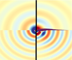
 $45$ degrees with the axis of symmetry.
Real part of the pressure component of neutral eigenvalues  $H_2$ (upper part) and
 $H_3$ (lower part) at
 $M=5 \times 10^{-2}$; (a)
 $\beta = 1$ and (b)
 $\beta = 2$.

Directivity patterns, in logarithmic scale, measured at  $r_x = \sqrt {r^{2} + x^{2}} = 150$. Results are shown for (a)
 $H_2$ and
 $\beta =1$; (b)
 $H_3$ and
 $\beta =1$; (c)
 $H_2$ and
 $\beta =2$; (d)
 $H_3$ and
 $\beta =2$. Colour legend: (—–, black)
 $M=10^{-2}$, (—–, red)
 $M= 2 \times 10^{-2}$ and (—–, yellow)
 $M= 5 \times 10^{-2}$.

7. Conclusion
The objective of the present paper was to investigate how the instability potential of a single jet passing through a hole in a thick plate, recently identified by Fabre et al. (Reference Fabre, Longobardi, Citro and Luchini2020) using LNSE in a strictly incompressible setting, manifests in a more realistic configuration involving compressibility. For this sake, we considered two generic situations. In the first situation, the upstream domain is a closed cavity and the downstream domain is an open space. This situation was chosen to check the conditional instability mechanism, requiring the existence of a conveniently tuned resonator. In the second situation, the two regions, upstream and downstream of the hole, are considered as open. This situation was chosen to check the purely hydrodynamical instability which is expected to exist even in the absence of a resonator.
The two cases have been analysed with an asymptotic method, which provides an instability criterion and an estimate for the amplification rate. The method consists, in a first step, in writing an impedance of the global system incorporating the hole impedance as computed by Fabre et al. (Reference Fabre, Longobardi, Citro and Luchini2020) and modelling the impedance of the upstream and downstream regions, and in a second step, in performing a Taylor expansion of this impedance around the real  $\omega$-axis to identify its zeros. The great advantage of the method is that the Mach number
 $M$ and the cavity volume
 $V_{in}$ appear as parameters in the model, so that a parametric study of the problem can be done entirely in terms of the Reynolds number and aspect ratio, therefore reducing the number of computational parameters from four to two.
The potential to accurately predict the instability properties via the asymptotic model is put into test in §§ 5.3 and 6 for the conditional and pure hydrodynamic cases, respectively. A cross-comparison with the results carried out with the compressible Navier–Stokes equations shows a good match between the two approaches. The impedance criterion has been employed to identify the regions of existence in the  $(Re, \chi )$ plane of a series of
 $C_i$,
 $i=1,2,3,4,\ldots$ modes. In addition to these acoustically compact modes, at larger Reynolds numbers, there exist unstable modes associated with higher-order modes of the cavity connected upstream (see figure 7 for an example of that phenomenon). The use of the impedance criterion for the characterisation of the compressibility effect in the pure hydrodynamical case is less accurate. We have observed that the estimations of the growth rate are relatively acceptable for the
 $H_2$ mode, but they are faulty for the
 $H_3$ mode, in particular for small length to diameter ratios. The inadequacy of the criteria to characterise this case can be attributed to the lack in the asymptotic model of the effect of the backward-travelling acoustic wave. These results suggest that a better modelling of the hydrodynamic-acoustic interaction is required to gain in accuracy. Finally, in § 6 we have examined the influence of the Mach number on the directivity pattern of the family of the pure hydrodynamical modes.
Declaration of interests
The authors report no conflict of interest.
Appendix A. Computation of the hole impedance thanks to incompressible LNSE
A.1. Incompressible Navier–Stokes equations
Under the hypothesis of acoustic compactness, discussed in § 2.3, the flow is assumed to be locally incompressible in the region of the hole, where the fluid motion is governed by the incompressible Navier–Stokes equations
 \begin{equation} \frac{\partial {} }{\partial t}\left[\begin{array}{c} \boldsymbol{u} \\ 0 \end{array} \right] ={\mathcal{N}S} \left( \left[\begin{array}{c} \boldsymbol{u} \\ p \end{array}\right] \right) = \left[\begin{array}{c} - \boldsymbol{u} \boldsymbol{\cdot} \boldsymbol{\nabla} \boldsymbol{u} - \boldsymbol{\nabla} p + {\textit{Re}}^{{-}1} \nabla^{2} \boldsymbol{u} \\ \boldsymbol{\nabla}\boldsymbol{\cdot} \boldsymbol{u} \end{array}\right].\end{equation}
The stability of the steady state  $[ \boldsymbol{u}_0, p_0 ]$ is investigated by using the linearized approach, in which the total flow field is decomposed into the sum of a steady base flow and a small time-harmonic perturbation as
 \begin{equation} \left[\begin{array}{c} \boldsymbol{u} \\ p \end{array} \right]= \left[\begin{array}{c} \boldsymbol{u_0} \\ p_0 \end{array}\right] + \varepsilon \left(\left[\begin{array}{c} \boldsymbol{\hat{u}} \\ \hat{p} \end{array}\right] {\rm e}^{-{\rm i}\omega t} + c.c. \right). \end{equation}
A.2. Incompressible Navier–Stokes equations – base-flow equations
The base flow is the solution of the steady version of the Navier–Stokes equations
 \begin{equation} {\mathcal{N}S} [\boldsymbol{u_0};p_0] = 0, \end{equation}
with the following set of boundary conditions:
 $$\begin{gather} \int_{{\mathcal \varGamma}_{in}} \boldsymbol{u_0} \boldsymbol{\cdot} \boldsymbol{n}\,{{\rm d}}S = Q_0, \end{gather}$$
 $$\begin{gather} p_0 = 0 \quad \text{on}\ \varGamma_{out}. \end{gather}$$
This problem is solved using a classical Newton iteration.
A.3. Linearized incompressible Navier–Stokes equations – forced problem
The linear perturbation is governed by the equations
 \begin{equation} - {\rm i}\omega \boldsymbol{\mathsf{B}} [\boldsymbol{\hat{u}}, \hat{p} ]^{\rm T} = \boldsymbol{\mathsf{LNS}}_0 ([\boldsymbol{\hat{u}}, \hat{p} ]^{\rm T}), \end{equation}
where  ${\boldsymbol{\mathsf{LNS}}}_0$ is the linearized Navier–Stokes operator around the base flow and
 $\boldsymbol{\mathsf{B}}$ is a weight operator defined as
 \begin{align} \boldsymbol{\mathsf{LNS}}_0 \left[\begin{array}{c} \boldsymbol{\hat{u}} \\ \hat{p} \end{array} \right] = \left[\begin{array}{c} - \left( \boldsymbol{u}_0 \boldsymbol{\cdot}\boldsymbol{\nabla} \boldsymbol{\hat{u}} + \boldsymbol{\hat{u}} \boldsymbol{\cdot}\boldsymbol{\nabla} \boldsymbol{u}_0 \right) - \boldsymbol{\nabla} \hat{p} + {\textit{Re}}^{{-}1} \nabla^{2} \boldsymbol{\hat{u}} \\ \boldsymbol{\nabla}\boldsymbol{\cdot} \boldsymbol{\hat{u}} \end{array}\right];\quad \boldsymbol{\mathsf{B}} = \left[\begin{array}{cc} 1 & 0 \\ 0 & 0 \end{array}\right]. \end{align}
Equation (A6a,b) is complemented with the following boundary conditions:
 $$\begin{gather} \int_{{\mathcal \varGamma}_{in}} \boldsymbol{\hat{u}} \boldsymbol{\cdot} \boldsymbol{n}\,{{\rm d}}S = q', \end{gather}$$
 $$\begin{gather} \hat{p}(x,r) = 0 \quad \text{on}\ \varGamma_{out}. \end{gather}$$
A non-zero perturbation of the flow rate  $q'$ is imposed, fixed arbitrarily, to
 $q'=1$. Equation (A7) thus leads to a non-homogeneous Dirichlet boundary condition at the inlet plane, treated by imposing a constant axial velocity
 $\hat {u}_x$. The problem can be symbolically written as
 \begin{equation} \left[ \boldsymbol{\mathsf{LNS}} + {\rm i} \omega {\boldsymbol{\mathsf{B}}} \right] [\boldsymbol{\hat{u}}; \hat{p} ]= \boldsymbol{F}, \end{equation}
where  ${\boldsymbol{\mathsf{LNS}}}$ is the linearized Navier–Stokes operator (implicitly containing the homogeneous boundary condition at the outlet), and
 $\boldsymbol{F}$ represents symbolically the non-homogeneous boundary condition at the inlet. This problem is non-singular and readily solved. Since
 $\hat {p}$ has been set to zero (without loss of generality) along the outlet boundary, the pressure drop
 $p'_{in}-p'_{out}$ can be extracted from
 $[\hat {\boldsymbol{u}}; \hat {p} ]$ by retrieving the mean value of the
 $\hat {p}$ component along the inlet boundary
 $\varGamma _{in}$ of the computational domain; such an operation can be written formally as
 $p'_{in} = {\boldsymbol{P}} [\hat {\boldsymbol{u}}, \hat {p} ]$, where
 $\boldsymbol{P}$ is a linear operator. The impedance is then ultimately deduced as
 $Z_h = {\boldsymbol{P}} \cdot {({\boldsymbol{\mathsf{LNS}}} + \textrm {i}\omega {\boldsymbol{\mathsf{B}}} )}^{-1} \cdot \boldsymbol{F}$.
Appendix B. Properties of the compressible steady state
As illustrated in figure 15, the base flow is characterised by a recirculation region originating from the upper corner of the hole. The pressure jump due to this recirculation can be represented by the so-called discharge coefficient (also called the vena contracta coefficient)  $\alpha _{vena} = {R_h^{2}}/{R_J^{2}}$, where
 $R_J$ is the effective radius of the jet. This function has been tabulated by Fabre et al. (Reference Fabre, Longobardi, Citro and Luchini2020) as a function of
 $Re$ and
 $\beta$ in the incompressible case. When taking into account the compressibility effects, the discharge coefficient (Bragg Reference Bragg1960) can be written in term of the dimensionless variables introduced in § 4.1 as
 \begin{equation} \alpha_{vena} = \frac{\dot{m}_0}{{\rm \pi} R_h^{2} \dfrac{1+\gamma M^{2} P_{in}}{\sqrt{T_{in}}}\dfrac{1}{M}\sqrt{\dfrac{2}{\gamma-1} \left[\left(\dfrac{1+\gamma M^{2}P_{in}}{1+\gamma M^{2}P_{out}}\right)^{{-}2/\gamma} - \left(\dfrac{1+\gamma M^{2}P_{in}}{1+\gamma M^{2}P_{out}}\right)^{-(\gamma+1)/\gamma}\right]}}, \end{equation}
which in the low Mach number limit can be approximated as
 \begin{equation} \alpha_{vena} = \frac{\dot{m}_0}{{\rm \pi} R_h^{2} \sqrt{\rho_{in} ( 2(P_{in}-P_{out}) - 3 M^{2}(P_{in}-P_{out})^{2}} }, \end{equation}
and it coincides with the one employed by Fabre et al. (Reference Fabre, Longobardi, Citro and Luchini2020) at the incompressible limit. Note that at large Reynolds numbers other simpler estimates exist, for instance, see the discussion by Gilbarg (Reference Gilbarg1960) for the compressible Borda tube, which has been revisited by Durrieu et al. (Reference Durrieu, Hofmans, Ajello, Boot, Aurégan, Hirschberg and Peters2001) and compared against experimental evidence. Figure 16(a) displays the effect of the Mach number on the discharge coefficient. It shows a good quantitative agreement with the theoretical estimation, and it weakly increases with the Mach number. Compressibility effects accelerate the bulk flow within the jet core, whereas the flow within the recirculation region hardly changes (see the evolution of the sensitivity with respect to the Mach number of the streamwise velocity in figures 16(b) and 15(b)). In addition, it has been observed that the shear layer thickness remains unchanged with a weak Mach number increase ( $M < 0.2$). In § 6 it is shown that an increase of the Mach number in the steady-state solution has a stabilizing effect, which can be attributed to an attenuated recirculation region.
Contour plot of the base flow  $\boldsymbol{q}_0$ for
 $\beta = 0.3$,
 $ {\textit {Re}} = 1400$ and
 $M=5\times 10^{-2}$. (a) Spatial evolution of the Mach number. (b) Spatial evolution of the sensitivity of the axial velocity with respect to the Mach number
 $\boldsymbol {\nabla }_M w_0$.

Discharge coefficient as a function of Mach number for several  $Re$ for
 $\beta = 0.3$. Dots correspond to computed values of
 $\alpha _{vena}$, lines correspond to the theoretical estimation, cf. Bragg (Reference Bragg1960). (b) Axial velocity profile of the sensitivity with respect to Mach number for
 $\beta =0.3$,
 $ {\textit {Re}} = 1600$,
 $M=10^{-1}$ at
 $z=0.2$.

Appendix C. Nyquist curve – Cauchy's argument principle
Let us review the use of the Nyquist criterion together with the drawing of Nyquist curves. In the absence of poles in the real axis, the Nyquist plot is drawn along the real axis. However, in the presence of a pole of the impedance in the real axis, one must take a contour that does not encircle the pole. In particular, the augmented system impedance possess a pole at  $\omega =0$, therefore, a complex contour that does not encircle zero is employed as the one depicted in figure 17(a). In the evaluation of the impedance, let us consider here without loss of generality the augmented system impedance
 $Z^{(a)}$ (either
 $Z^{(a)} = Z_a$ or
 $Z^{(a)} = Z_b$) along the contour
 $\varGamma$, i.e.
 $Z^{(a)}(\varGamma )$, which provides a direct evaluation of the stability of the system. Provided that the contour of integration does not encircle any pole of the system, which is satisfied by construction, the number of times that the curve
 $Z^{(a)}(\varGamma )$ encircles the origin in the counterclockwise direction determines the number of zeros in the area surrounded by the contour
 $\varGamma$. In the condition that the contour of integration
 $\varGamma$ encloses the unstable complex plane, then any encirclement of the origin implies that the system is unstable. To illustrate this, let us consider the Nyquist curve represented in figure 17(b), where the curve
 $Z^{(a)}(\varGamma )$ is oriented counterclockwise, and it encircles twice the origin: this implies that the system has two unstable zeros. A more careful evaluation reveals that this corresponds to a pair of conjugated complex zeros.
(a) The complex contour  $\varGamma$ of integration enclosing the unstable complex plane, where Cauchy's argument principle is applied. (b) Nyquist curve for the augmented system impedance along
 $\varGamma$.

Additionally, impedance values for real  $\omega$ can also provide an estimation of the complex zeros whenever
 $\textrm {Im}(\omega )$ is of small magnitude. Here, let us detail the procedure followed in § 3.3.1. We consider the case where the Nyquist curve is found near the origin. The first scenario corresponds to a complex frequency
 $\omega = \omega _R + \textrm {i}\omega _I = \omega _0 + \varepsilon \omega _1$, where
 $\omega _0, \omega _R, \omega _I$ are real values,
 $\omega _1$ is considered to be complex and a small real parameter
 $\varepsilon \ll 1$.
Provided the impedance  $Z^{(a)}(\omega ) = \textrm {Re}( Z^{(a)}(\omega ) ) + \textrm {i}\textrm {Im}( Z^{(a)}(\omega ) ) = Z^{(a)}_R(\omega ) + \textrm {i} Z^{(a)}_I(\omega )$ is analytic, the first-order Taylor expansion at
 $\omega _0$ provides
 \begin{equation} 0 = Z^{(a)}(\omega) = Z^{(a)}(\omega_0) + \left(\frac{{{\rm d}}Z^{(a)}}{{{\rm d}} \omega}\right)_{\omega=\omega_0}(\omega - \omega_0) + R_1(\omega), \end{equation}
where  $R_1(\omega )$ is the remainder of the Taylor expansion. The remainder of the expansion can be shown to be bounded, for instance, using Cauchy's integral formula and the maximum principle (see, for instance, Rudin Reference Rudin1987) yields
 \begin{equation} |R_1(\omega)| \leq M_r \frac{|\omega - \omega_0|^{2}}{ r (r - |\omega - \omega_0|)} \leq M_r \frac{\eta^{2}}{1-\eta},\quad \text{with } M_r \equiv \max_{|\omega-\omega_0|=r} |Z^{(a)}(\omega)| \end{equation}
for  $|\omega - \omega _0| < r$ and
 ${|\omega - \omega _0|}/{r}\leq \eta < 1$, where we have assumed that the impedance function is holomorphic in a closed disk of radius
 $r$ of the complex plane. Therefore, the function
 ${R_1(\omega )}/{(\omega - \omega _0)}$ is also analytic within the disk. In such a way we can approximate the value of zero
 $\omega$ as
 \begin{align} \omega - \omega_0 &= \frac{Z^{(a)}(\omega_0)}{\displaystyle \left(\frac{{{\rm d}}Z^{(a)}}{{{\rm d}} \omega}\right)_{\omega = \omega_0} + \frac{R_1(\omega)}{\omega - \omega_0}} \approx \frac{Z^{(a)}(\omega_0)}{\displaystyle \left(\frac{{{\rm d}}Z^{(a)}}{{{\rm d}} \omega}\right)_{\omega = \omega_0}} \nonumber\\ &= \frac{Z^{(a)}_R(\omega_0) + {\rm i}Z^{(a)}_I(\omega_0)}{\displaystyle \left(\frac{\partial Z^{(a)}_R (\omega)}{\partial \omega_R}\right)_{\omega = \omega_0} + {\rm i}\left(\frac{\partial Z^{(a)}_I (\omega)}{\partial \omega_R}\right)_{\omega = \omega_0}}, \end{align}
where the error of the approximation is
 \begin{equation} \epsilon \leq \left|\frac{Z(\omega_0)}{\displaystyle \left(\frac{{{\rm d}}Z}{{{\rm d}} \omega} \right)_{\omega = \omega_0}}\right|\frac{\eta'}{1-\eta'}, \end{equation}
with  $\eta ' = {|R_1(\omega )|}/{|\omega - \omega _0|} / | ({{\textrm {d}}Z}/{{\textrm {d}} \omega } )_{\omega = \omega _0} |$, because the radius of convergence of the rational complex function
 ${1}/{(({{\textrm {d}}Z}/{{\textrm {d}} \omega })_{\omega = \omega _0}+z)}$ is equal to
 $|({{\textrm {d}}Z}/{{\textrm {d}} \omega })_{\omega = \omega _0}|$. Thus, the approximation (C3) converges uniformly far from the critical points of the impedance. Furthermore, it provides good estimates whenever
 $|Z(\omega _0)| \sim \varepsilon \ll 1$ and
 ${|\omega - \omega _0| \sim \varepsilon \ll 1}$, which is the motivation to the condition (i) and the expansion in frequency in § 3.3.1. Finally, note that (C3) could be used as a step in a Newton iteration, whenever the initial guess
 $\omega _0$ is far from the zero of the impedance.
Multiplication by the complex conjugate of the denominator in (C3) leads to
 \begin{equation} \varepsilon \omega_1 \approx \frac{\left(Z^{(a)}_R(\omega_0) + {\rm i}Z^{(a)}_I(\omega_0)\right) \left(\displaystyle \left(\frac{\partial Z^{(a)}_R (\omega)}{\partial \omega_R}\right)_{\omega = \omega_0} - {\rm i}\left(\frac{\partial Z^{(a)}_I (\omega)}{\partial \omega_R}\right)_{\omega = \omega_0}\right)}{\displaystyle \left(\left(\frac{\partial Z^{(a)}_R (\omega)}{\partial \omega_R}\right)_{\omega = \omega_0}\right)^{2} + \left(\left(\frac{\partial Z^{(a)}_I (\omega)}{\partial \omega_R}\right)_{\omega = \omega_0}\right)^{2}}. \end{equation}
Finally, one could split (C5) in real and imaginary parts, this yields the expression for  $\omega _R$,
 \begin{equation} \varepsilon \text{Re}(\omega_1) = \omega_R - \omega_0 \approx \frac{\left( Z^{(a)}_R(\omega_0) \displaystyle \left(\frac{\partial Z^{(a)}_R (\omega)}{\partial \omega_R}\right)_{\omega = \omega_0} + Z^{(a)}_I(\omega_0) \left(\frac{\partial Z^{(a)}_I (\omega)}{\partial \omega_R}\right)_{\omega = \omega_0}\right)}{\displaystyle \left(\left(\frac{\partial Z^{(a)}_R (\omega)}{\partial \omega_R}\right)_{\omega = \omega_0}\right)^{2} + \left(\left(\frac{\partial Z^{(a)}_I (\omega)}{\partial \omega_R} \right)_{\omega = \omega_0}\right)^{2}}, \end{equation}
and for  $\omega _I$,
 \begin{equation} \varepsilon \text{Im}(\omega_1) = \omega_I \approx \frac{\left(Z^{(a)}_I(\omega_0) \displaystyle \left(\frac{\partial Z^{(a)}_R (\omega)}{\partial \omega_R}\right)_{\omega = \omega_0} - Z^{(a)}_R(\omega_0) \left(\frac{\partial Z^{(a)}_I (\omega)}{\partial \omega_R}\right)_{\omega = \omega_0}\right)}{\displaystyle \left(\left(\frac{\partial Z^{(a)}_R (\omega)}{\partial\omega_R}\right)_{\omega = \omega_0}\right)^{2} + \left(\left(\frac{\partial Z^{(a)}_I(\omega)}{\partial \omega_R}\right)_{\omega = \omega_0}\right)^{2}}. \end{equation}
Appendix D. Frequency selection argument
This appendix provides an argument explaining the quantification of the eigenvalues observed for the cavity/open configuration.
The frequency of the sound generated is selected by considering the two elements that compose the feedback loop of a class III aerodynamic whistle: the hydrodynamic-acoustic wave interaction and the acoustic resonator. In this kind of mechanism, we can distinguish two feedback loops, a first loop composed of the interaction of a hydrodynamic instability with an acoustic wave and a second one which accounts for the interaction of the first feedback loop with the acoustic resonator. A hydrodynamic-acoustic wave interaction develops whenever the shear layer of the jet is unstable and the jet acts as a source of energy, which occurs when the resistance of the hole is negative. The shear layer instability is triggered at the leftmost corner of the hole, disturbances grow along the hole; however, in the case when the shear layer is not sufficiently unstable (so self-sustained oscillations arise by pure hydrodynamical arguments) it requires an acoustic wave to close the loop, which is an instantaneous process in the low Mach number limit. For acoustically compact source regions, the frequency selection of this mechanism is dominated by the hydrodynamic instability, because the travel time of the acoustic wave is of lower order of magnitude. Secondly, the cavity acts a resonator, selecting a set of discrete frequencies among those associated with a negative resistance.
In the present configuration, there exist four branches of instability, each of them denoted as  $C_n$ for
 $n=1,2,3,4$, which are characterised by a nearly constant Strouhal number
 \begin{equation} St^{(n)}_{\beta} = \frac{\omega^{(n)} \beta}{2 {\rm \pi}} \end{equation}
as  $\beta$ is varied. The characteristic frequency of
 $C_n$ branches is related by a frequency shift
 $St^{(n)}_{\beta } = St^{(n-1)}_{\beta } + {\rm \Delta} St_{\beta }$, where
 ${\rm \Delta} St_{\beta } \approx [0.6,0.7]$. This frequency shift may be estimated if one realizes that the global instability is the result of the constructive interaction between two travelling waves: a downstream-travelling wave, which is excited about the hole lip and propagates around the jet core position, and an upstream-travelling wave that propagates backwards. The non-local constructive interaction of such waves gives rise to a self-sustained global in time instability, which, in some circumstances, is able to radiate an intense acoustic field.
In the following analysis we reconsider the discharge coefficient  $\alpha _{vena} = \sqrt {{\rho U_M^{2}}/{2(P_{in} - P_{out})}}$, which can be thought of as a measure of the vena contracta phenomenon, assuming that the jet contracts to a top-hat jet with constant velocity
 $U_J$ and radius
 $R_J$. Then applying Bernouilli law, one obtains
 $\alpha _{vena} = {U_M}/{U_J} = {{\rm \pi} R_J^{2}}/{{\rm \pi} R_h^{2}}$ that was introduced in Fabre et al. (Reference Fabre, Longobardi, Bonnefis and Luchini2019) in the discussion of the work of Howe (Reference Howe1979), which is classically associated with the pressure loss across the aperture, and it relates the mean velocity
 $U_M$ with the jet velocity
 $U_J$. In Fabre et al. (Reference Fabre, Longobardi, Bonnefis and Luchini2019, § 2.5 and Appendix A) the importance of the vena contracta coefficient
 $\alpha _{vena}$ and the actual value of the phase velocity of the Kelvin–Helmholtz instability, where the phase velocity depends on the frequency
 $\omega$ but which is around
 $U_c = U_J/2$ for sufficiently high
 $\omega$. The value of the discharge coefficient tends asymptotically to
 $\alpha _{vena} \to 0.61$ for large
 $Re$; however, in the range of Reynolds numbers where transition occurs
 $\alpha _{vena}$ is maximal and takes values
 $\alpha _{vena} \in [0.7,0.76]$. In the following, we consider a constant discharge coefficient
 $\alpha _{vena} = 0.76$, which was the value reported in Fabre et al. (Reference Fabre, Longobardi, Citro and Luchini2020, figure 5) for most of
 $\beta$ in the range of Reynolds numbers where the transition occurs.
In order to estimate the frequency shift  ${\rm \Delta} St_{\beta }$ let us consider the travel time of each travelling wave past the hole. The hydrodynamic travelling wave takes
 ${\rm \Delta} \tau _{KH} = {L_h}/{U_c} = {2 \alpha _{vena} L_h}/{U_M}$ and the acoustic wave
 ${\rm \Delta} \tau _{ac} = {M L_h}/{U_M}$; therefore, the total travelling time
 \begin{equation} {\rm \Delta} \tau = {\rm \Delta} \tau_{KH} + {\rm \Delta} \tau_{ac} = \frac{L_h (2 \alpha_{vena} +M)}{U_M} \approx {2 \alpha_{vena}} \frac{L_h}{U_M}, \quad f^{(n)} = \frac{2n-1}{2 {\rm \Delta} \tau},\quad {\rm \Delta} f = \frac{1}{{\rm \Delta} \tau}, \end{equation}
where it is considered that  $M \ll 1$ and the convective velocity of the hydrodynamic perturbation is
 $\frac {2\alpha _{vena}}{U_M}$ as it is displayed in figure 19. Thus, the associated Strouhal shift
 \begin{equation} {\rm \Delta} St_{\beta} = \frac{{\rm \Delta} f L_h}{U_M} \approx \frac{1}{2 \alpha_{vena}}. \end{equation}
Similarly, the Strouhal frequency of each  $C_n$ branch is estimated as
 \begin{equation} St^{(n)}_\beta = \frac{2n-1}{4 \alpha_{vena}},\quad n = 1,2,3 \ldots. \end{equation}
(a) Thresholds of the conditional instabilities  $C_1$,
 $C_2$,
 $C_3$ and
 $C_4$ as a function of
 $\beta$ and
 $Re$. (b) Strouhal evolution with
 $\beta$. Solid lines are the boundaries of the conditional stability computed with incompressible LNSE and dashed lines are the estimation with
 $\alpha _{vena} = 0.76$.

Diagram of the non-local interaction leading to global instability.

In the previous reasoning, it has been implicitly assumed that only odd mode structures as those depicted in Fabre et al. (Reference Fabre, Longobardi, Citro and Luchini2020, figure 9) lead to a conditional instability. The superposition of the base flow with odd modes (respectively even) at the instant of the cycle where the flow rate through the hole is maximum results in an upward (respectively downward) displacement of the shear layer, thus, pressure is increased (respectively decreased) in the presence of odd modes (respectively even). This implies that the hole impedance is negative, which is the criterion of existence of conditional stability.
Finally, let us discuss the influence of compressibility regarding modifications in frequency at the threshold of instability for each of the unstable modes. Compressibility induces a weak variation in the vena contracta coefficient, see figure 16(a), while the threshold of instability is significantly modified for a given value of  $\beta$ near the left asymptote for conditional instabilities (figure 18a) and hydrodynamic instabilities (figure 11a). Thus, for short holes
 $\beta$ (here short refers to a value of
 $\beta$ near a vertical asymptote of the corresponding instability), the critical Reynolds number is considerably modified by compressible effects, which in turn induces a change in the vena contracta coefficient (more important than the variation of the vena contracta by compressibility at constant Reynolds number). For those cases, one could evaluate the shift in frequency
 $\delta |_{M} {\rm \Delta} St_{\beta } = {\rm \Delta} St_{\beta }(M+{\rm \Delta} _M) - {\rm \Delta} St_{\beta }(M)$ as
 \begin{equation} \delta|_{M} {\rm \Delta} St_{\beta} ={-} \frac{2\left(\alpha_{vena} (Re_c(M+{\rm \Delta} M), M +{\rm \Delta} M) - \alpha_{vena}(Re_c(M), M)\right) + {\rm \Delta} M }{\left(2 \alpha_{vena}(Re_c(M), M) + M\right)^{2}}, \end{equation}
where the first term, the variation in the vena contracta due to a variation in Mach number, is negligible with respect to the variation in Mach number for long holes, and thus, the variation of frequency for those instabilities is of lesser importance.
Appendix E. Computational domains and absorbing boundary layer
This section discusses the design of computational domains used for the computation of steady states and eigenmodes with the full compressible formulation, and steady states and the forced harmonic response with the incompressible formulation. The computational strategy must be designed in such a way as to avoid the presence of spurious eigenvalues/eigenmodes. The creation of meshes for the full compressible formulation follows a block-structured strategy, similar to the one sketched in figure 4. The domain is divided into three regions: an inner region with the highest vertex density, a mid region with intermediate vertex density and a coarser region for the absorbing layer. Meshes employed for the incompressible case are composed of two regions, a physical domain with the highest vertex density and a coarser region for the absorbing layer. Table 1 lists a number of computational meshes employed in this study ( $\mathbb {M}_2$,
 $\mathbb {M}_3$,
 $\mathbb {M}_4$ and
 $\mathbb {M}_5$ for the full compressible case, and
 $\mathbb {M}_1$ for the incompressible case). However, such a list is not exhaustive because in addition to the block-strategy refinement, the computational domain has been locally refined following an adaptive local refinement procedure, where the metric for the refinement is based on the steady state and on the eigenmodes (respectively steady state and forced harmonic response in the incompressible case), cf. Hecht (Reference Hecht2012) and Fabre et al. (Reference Fabre, Citro, Ferreira, Bonnefis, Sierra, Giannetti and Pigou2018).
Meshes used for cases where the complex mapping technique is adopted. Note: the smooth transition functions are defined as  $g_z(Z) = \tanh ([{(Z-Z_0)}/{L_c}]^{2})$ and
 $g_r(R) = \tanh ([{(R-R_0)}/{R_c}]^{2})$. In the following,
 $L_{max} = z_{-\infty } + z_{CM} = z_{\infty } + z_{CM}$ and
 $R_{max} = r_\infty + r_{CM}$ (figure 4).

The absorbing boundary layer corresponds to the complex mapping technique (Sierra et al. Reference Sierra, Fabre and Citro2020) where a coordinate transformation  $\mathcal {G}$ is defined as follows:
 \begin{equation} \left.\begin{gathered} \mathcal{G}_{z}:\mathbb{R} \to \mathbb{C} \quad \text{such that}\ z= \mathcal{G}_z(Z) = \left[1 + {\rm i} \gamma_{z,c} g_z(Z) \right] Z, \\ \mathcal{G}_{r}:\mathbb{R} \to \mathbb{C} \quad \text{such that}\ r= \mathcal{G}_r(R) = \left[1 + {\rm i} \gamma_{r,c} g_r(R) \right] R. \end{gathered}\right\} \end{equation}
Here  $g_z(Z)$ (respectively
 $g_r(R)$) has to be chosen as a smooth function such as
 $g_z(Z)= 0$ for
 $Z< Z_0$ and
 $g_z(Z) \approx 1$ for
 $Z>Z_0+L_c$ up to
 $Z_{max}$. The complex mapping acts on a finite region of length
 $z_{CM} = Z_{max} - ( Z_0 + L_c )$. The function
 $g_z$ is defined as
 $g_z(Z) = \tanh ([{(Z-Z_0)}/{L_c}]^{2})$. The application of this map to the linearized Navier–Stokes requires that each spatial derivative, within the complex mapped region, is modified as
 \begin{equation} \frac{\partial }{\partial z} \equiv \mathcal{H}_z \frac{\partial }{\partial Z}\quad \mbox{with}\ \mathcal{H}_z(Z) = {\left(\frac{\partial \mathcal{G}_z}{\partial Z} \right)}^{{-}1}. \end{equation}
An example of parameters for the usage of the complex mapping layer for the incompressible case is listed in table 1 ( $\mathbb {M}_1$). In the full compressible formulation, one must pay particular attention to the extension of the complex mapping region, which here is selected to cover at least two acoustic wavelengths, i.e.
 $z_{CM} = r_{CM} > {1}/{St\, M}$. For instance, the largest acoustic wavelength in this study corresponds to the validation case in § 5.1, where
 $\lambda _{ac} \approx 600$ (
 $St \approx 1/3$ and
 $M = 5 \times 10^{-3}$), for which
 $\mathbb {M}_5$ is an appropriate choice.


 Open access

