1. Introduction
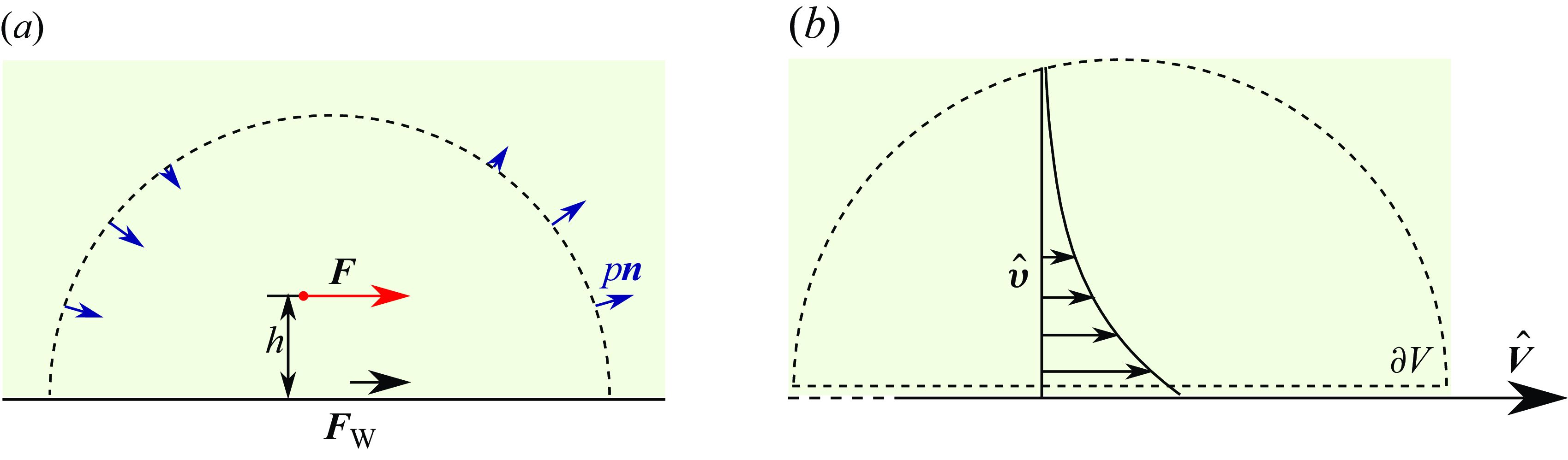
In the absence of of inertia, fluids at low Reynolds numbers are always in a state of force balance: the sum of volume forces, surface forces and the stress integrated over a closed surface always equals zero. In confined geometries, the force balance can take a surprising form. A notable example is the flow due to a point force inside a long pipe with a no-slip boundary (Brenner Reference Brenner1959; Liron & Shahar Reference Liron and Shahar1978). The external force leads to a pressure difference between the two ends of the pipe (figure 1 a). Depending on the radial position of the point force, the pressure difference, multiplied by the cross-section area of the pipe, can exceed the original force by a factor of 2 (Pliskin & Brenner Reference Pliskin and Brenner1963; Mondy et al. Reference Mondy, Tetlow, Graham, Abbott and Brenner1997). The remainder of the force is contributed by the force on the wall of the pipe, which changes its sign at a certain position of the applied force. A related result was found for a Stokeslet between two parallel plates (Škultéty & Morozov Reference Škultéty and Morozov2020).
The Brinkman equation (Brinkman Reference Brinkman1949a ,Reference Brinkman b )
 \begin{equation} \eta (\Delta \boldsymbol {v}-\alpha ^2 \boldsymbol {v})-\nabla p+\boldsymbol {f}=\boldsymbol {0}\,, \end{equation}
along with the incompressibility condition
 $\nabla \cdot \boldsymbol {v}=0$
, describes the flow of a fluid through a porous medium. Here,
 $\eta$
is the dynamic viscosity of the Newtonian fluid and
 $\alpha ^2$
represents the impermeability of the porous medium, with dimensions of (length)
 $^{-2}$
. The density of external forces acting on the fluid is denoted by
 $\boldsymbol {f}$
. Equivalently, it can also be expressed as a continuity equation for the stress tensor
 $\boldsymbol {\sigma }=-p \boldsymbol {I}+ \eta (\nabla \boldsymbol {v} + (\nabla \boldsymbol {v})^T)$
:
 \begin{equation} \nabla \cdot \boldsymbol {\sigma }-\eta \alpha ^2\boldsymbol {v}+\boldsymbol {f}=\boldsymbol {0} \,. \end{equation}
The force balance therefore needs to take into account the momentum exchange between the fluid and the medium. The force balance equation on a volume of fluid
 $\mathcal V$
is obtained by applying the divergence theorem to (1.2) and reads
 \begin{equation} \oint _{\partial \mathcal V} \boldsymbol {\sigma }\cdot \boldsymbol {n} \, {{\mathrm {d}}} S + \int _{\mathcal V} (\boldsymbol {f} -\eta \alpha ^2 \boldsymbol {v}) \, {{\mathrm {d}}} V =\boldsymbol {0}\,, \end{equation}
with
 $\boldsymbol {n}$
as a unit normal vector pointing outward. In this paper, we discuss the cumulative force balance in Brinkman flows under different types of confinement. We discuss the application of the results to different kinds of cytoplasmic flows.
Point force in a pipe. (a) Force balance: the external force
 $F$
is distributed to the force on the wall
 $F_{\textrm{W}}$
and the force due to pressure difference
 $F_{ {P}}=\pi R^2 \Delta p$
. The direction of the force on the walls changes with the radial position of the force. (b) Pressure-driven flow through a pipe with a Brinkman fluid is used as an auxiliary problem when applying the reciprocal theorem. (c) Induced pressure difference as a function of the distance
 $h$
of the force from the tube’s axis, as given by (2.8). The dashed line represents the limit
 $\alpha \to \infty$
. (d) Streamlines around a point force acting at the centre of the channel (
 $h=0$
). At small values of
 $\alpha R$
, the flow shows a series of viscous tubular eddies which disappear at
 $\alpha R\approx 4.7$
.

2. Examples of force balance
The discussion of specific cases follows the level of confinement. We begin with the flow induced by a point force in an infinite pipe, akin to the solution by Liron & Shahar (Reference Liron and Shahar1978), but with a Brinkman medium instead. We continue with the point force in the presence of a wall, extending the classical solution of Blake (Reference Blake1971), with a force balance specifically discussed by Škultéty & Morozov (Reference Škultéty and Morozov2020). Finally, we proceed with a force inside a porous sphere with open boundaries (i.e. surrounded by free fluid), as well as no-slip spherical confinement. All solutions are determined by the application of the Lorentz reciprocal theorem, which greatly simplifies the calculation of cumulative forces. We also validate and illustrate the results with explicit exact solutions for some cases.
2.1. Material force in confined flows
We begin with a note on the material force, i.e. the force the fluid exerts on the porous medium,
 \begin{equation} \boldsymbol {F}_{\text {M}}=\int _{\mathcal {V}} \eta \alpha ^2 \boldsymbol {v} \, {{\mathrm {d}}} V, \end{equation}
in a confined flow with zero normal velocity,
 $ \boldsymbol {v}\cdot \boldsymbol {n}=0$
, at the outer boundary
 $\partial \mathcal V$
. By applying the divergence theorem to the quantity
 $(\boldsymbol {e}\cdot \boldsymbol {x}) \boldsymbol {v}$
with an arbitrary unit vector
 $\boldsymbol {e}$
and noting that
 $\nabla \cdot ((\boldsymbol {e}\cdot \boldsymbol {x}) \boldsymbol {v})= \boldsymbol {e}\cdot \boldsymbol {v}$
for
 $\nabla \cdot \boldsymbol {v}=0$
, we obtain
 \begin{equation} \boldsymbol {e}\cdot \int _{\mathcal {V}} \boldsymbol {v} \, {{\mathrm {d}}} V = \oint _{\partial \mathcal {V}} (\boldsymbol {e}\cdot \boldsymbol {x}) \boldsymbol {v} \cdot \boldsymbol {n} \, {{\mathrm {d}}} S =0\,. \end{equation}
Because the equality holds for any
 $\boldsymbol {e}$
, it follows that
 \begin{equation} \int _{\mathcal {V}} \boldsymbol {v} \, {{\mathrm {d}}} V =\boldsymbol {0} \end{equation}
for any confined flow and, therefore, the total force acting on the porous material vanishes,
 $\boldsymbol {F}_{\text {M}}=\boldsymbol {0}$
.
2.2. Point force in a pipe
The first example consists of a point force
 $F$
inside an infinitely long pipe with radius
 $R$
that is filled with a porous medium (figure 1
a). The force is acting in axial direction at distance
 $h$
from the axis of the pipe. We disregard any radial components of the force
 $F$
, because it is clear from symmetry arguments that they will act on the wall of the tube alone, without contributing to the long-range pressure difference.
To apply the Lorentz reciprocal theorem, we first solve the auxiliary problem, which is a pressure-driven flow through a pipe containing a Brinkman medium (figure 1
b). The fluid is therefore described by the Brinkmanequation (1.1), along with the condition of incompressibility
 $\nabla \cdot \boldsymbol {\hat v}=0$
(the hatted quantities are used to distinguish the auxiliary from the main problem). The pipe is oriented along the
 $z$
-axis. At the walls, the no-slip condition
 $\boldsymbol {\hat v}=\boldsymbol 0$
applies and the whole tube is subject to a negative pressure gradient,
 $G=-\mathrm {d} \hat p / \mathrm {d} z \gt 0$
. We write the Brinkman equation in cylindrical coordinates
 \begin{equation} \frac {1}{\rho } \frac {\mathrm {d} }{\mathrm {d} \rho } \left ( \rho \, \frac {\mathrm {d} \hat {v}_z}{\mathrm {d} \rho } \right ) - \alpha ^2 \hat {v}_z + \frac {G}{\eta } = 0 \, . \end{equation}
The boundary condition states
 $ \hat {v}_z(\rho = R) = 0$
. The solution for the axial velocity is
 \begin{equation} \hat {v}_z = \frac {G}{\alpha ^2 \eta } \left ( 1 - \frac {I_0(\alpha \rho )}{ I_0(\alpha R) } \right ) \, , \end{equation}
with
 $I_n(x)$
denoting the
 $n$
th-order modified Bessel function of the first kind (Abramowitz & Stegun Reference Abramowitz and Stegun1972). The volume flow rate through the pipe is
 \begin{equation} \hat Q = \int _0^R \hat v_z (\rho ) \, 2\pi \rho \, {{\mathrm {d}}}\rho = \frac {\pi R^2 G}{\alpha ^2 \eta } \frac {I_2(\alpha R)}{ I_0(\alpha R) } \;. \end{equation}
In the limit
 $\alpha \to 0$
, corresponding to the Stokes flow regime, we can use the series expansion
 $I_0(x)= 1+ x^2/4 + \mathcal {O}(x^4)$
,
 $I_2(x)= x^2/8 + \mathcal {O}(x^4)$
and recover the classical parabolic velocity profile of the Hagen–Poiseuille flow with
 $\hat v _z=G (R^2-r^2) /(4\eta )$
and
 $\hat Q=\pi R^4 G/(8\eta )$
.
We now apply the Lorentz reciprocal theorem (derived for Brinkman fluids in Appendix A) with the pressure driven flow as auxiliary problem. The reciprocal theorem states
 \begin{equation} \int _{\mathcal \partial \mathcal V} \boldsymbol {v}\cdot \hat {\boldsymbol \sigma } \cdot \boldsymbol {n} \, {{\mathrm {d}}} S + \int _{\mathcal V} \boldsymbol {v} \cdot \boldsymbol {\hat f} \, {{\mathrm {d}}} V= \int _{\mathcal \partial \mathcal V} \boldsymbol {\hat v}\cdot \boldsymbol \sigma \cdot \boldsymbol {n} \, {{\mathrm {d}}} S + \int _{\mathcal V} \boldsymbol {\hat v} \cdot \boldsymbol {f} \, {{\mathrm {d}}} V \,. \end{equation}
The integration surface
 $\partial \mathcal V$
runs along the wall of the pipe and is closed at
 $z=\pm \infty$
(figure 1
b). Because both velocities are zero at the walls, all surface integrals vanish there. At the ends of the pipe, the left surface integral vanishes because
 $\boldsymbol {v}\to \boldsymbol 0$
, but the right gives
 $-\hat Q \Delta p$
, where
 $\Delta p=p(z\to \infty )-p(z\to -\infty )$
is the pressure difference build-up in the main problem. We know that the pressure at both ends needs to be constant across the tube because of the vanishing velocity. The left volume integral also vanishes because
 $\boldsymbol {\hat f}=\boldsymbol {0}$
by definition. This leads to a relationship for the pressure difference
 \begin{equation} \Delta p=\frac {F \hat v_z(h)}{\hat Q}= \frac {F}{\pi R^2} \frac {I_0(\alpha R)-I_0(\alpha h)}{I_2(\alpha R)}\;. \end{equation}
In the limit
 $\alpha \to 0$
, the relation simplifies to
 $\Delta p=2 F (1-h^2/R^2)/(\pi R^2)$
, in agreement with the exact flow solution (Brenner Reference Brenner1959; Liron & Shahar Reference Liron and Shahar1978) and also the lubrication approximation by Navardi & Bhattacharya (Reference Navardi and Bhattacharya2010). Note that the reciprocal theorem allowed us to obtain this result with a much shorter and simpler derivation compared with the explicit solutions in the references above.
The resulting radial dependence is shown in figure 1(c). Whereas the Brinkman medium always reduces the pressure if the force is near the axis of the channel, the opposite is the case in the proximity of the wall, where an increased value of
 $\alpha$
leads to a higher
 $\Delta p$
.
Because of the rapid fall-off of the velocity with the distance along the pipe, the pipe can be effectively seen as confined and the force on the porous material is zero. Force balance therefore implies that the force exerted by the fluid on the walls is
 \begin{equation} F_{\text {W}}= F-\pi R^2 \Delta p=F\left ( 1 - \frac {I_0(\alpha R)-I_0(\alpha h)}{I_2(\alpha R)} \right ). \end{equation}
As in the Stokes fluid, the force on the wall changes direction: it is parallel to
 $F$
when the external force acts close to the wall, but antiparallel when it is in the centre of the pipe.
Although we only consider an infinitely long tube here, the solution for a length that is finite, but still much larger than the diameter, can easily be obtained by superposition. Another possible extension is the mobility matrix of two particles in the pipe. For Stokes fluids, it has been shown that the off-diagonal elements expressing hydrodynamic interactions depend on the length of the tube, but not on the distance between the particles (Misiunas et al. Reference Misiunas, Pagliara, Lauga, Lister and Keyser2015).
2.3. Point force in the proximity of a plane
We now study the force exerted on an infinite plane by a force acting parallel to it at some distance
 $h$
(figure 2
a). The auxiliary problem consists of the plane itself moving tangentially with velocity
 $\hat {\boldsymbol {V}}$
while the porous medium itself does not move (figure 2
b). The Brinkman equation for the auxiliary problem reduces to
 \begin{equation} (\partial _z^2 -\alpha ^2) \hat {\boldsymbol {v}}=\boldsymbol {0} \, , \end{equation}
with the boundary condition
 $\hat {\boldsymbol {v}}=\hat {\boldsymbol {V}}$
at
 $z=0$
and is solved as
 \begin{equation} \hat {\boldsymbol {v}}=\hat {\boldsymbol {V}} e^{-\alpha z}\,. \end{equation}
(a) Point force
 $\boldsymbol F$
on the Brinkman fluid in the presence of a no-slip wall. The force is distributed over the force on the wall
 $\boldsymbol {F}_{\textrm{W}}$
, the force on the porous medium
 $\boldsymbol {F}_{\textrm{M}}$
and force due to the pressure difference. (b) In the auxiliary problem, the wall itself is moving with the velocity
 $\hat {\boldsymbol {V}}$
.

We now apply the Lorentz reciprocal theorem to the half-space containing the Brinkman fluid. The integration surface contains the plane and the upper hemisphere at infinite distance (dashed line in figure 2
b). Because both
 $\hat {\boldsymbol v}$
and
 $\boldsymbol v$
converge to 0 sufficiently fast at large distances, the surface integrals over the hemisphere vanish. The reciprocal theorem then states that
 \begin{equation} \int \hat {\boldsymbol V} \cdot \boldsymbol {\sigma }\cdot \boldsymbol {e}_z \, {{\mathrm {d}}} S - \hat {\boldsymbol {v}} \cdot \boldsymbol F = 0 \end{equation}
leading to
 $ \hat {\boldsymbol V} \cdot \boldsymbol {F}_{\text {W}}= \hat {\boldsymbol {v}}\cdot \boldsymbol F$
. The horizontal force exerted by the fluid on the plane is therefore
 \begin{equation} F_{\text {W}} = F e^{-\alpha z}\,. \end{equation}
The long-range nature of the flow and pressure (calculated explicitly in (C18)) has the consequence that the integral
 $\int p \boldsymbol {n} \,{{\mathrm {d}}} S$
does not have a defined limit when the boundary is infinitely far from the force. Therefore, it is not possible to state which part of the force is carried by pressure and which part by the porous medium, unlike the force on the wall. However, the force due to the pressure vanishes in the Stokes limit
 $\alpha \to 0$
, as already noted by Blake (Reference Blake1971). A related problem appears in a Stokes fluid between two plates, which becomes related to a two-dimensional (2-D) Brinkman fluid in the far-field regime. Although the pressure contribution to the horizontal force balance was determined by Škultéty & Morozov (Reference Škultéty and Morozov2020), we note that the exact result depends on the way how the integration area approaches an infinite plane and is therefore not uniquely defined.
2.4. Point force inside a sphere with open boundaries
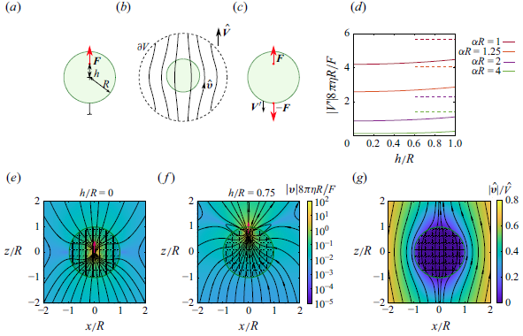
In this section, we consider an external point force acting on the fluid inside a porous sphere, immersed in a Stokes fluid of the same viscosity (figure 3 a). The porous medium itself is fixed in the laboratory frame.
(a) Force
 $\boldsymbol {F}$
acting axisymmetrically on the Brinkman fluid inside a porous sphere at a fixed position in laboratory frame and embedded in a Stokes fluid. (b) The same sphere, subject to an external flow with velocity
 $\hat {\boldsymbol {V}}$
, is used as an auxiliary problem. (c) The porous sphere is free to move and subject to a pair of opposite forces, one acting on the Brinkman fluid and one on the sphere. (d) Velocity
 $\boldsymbol {V}^\prime$
of the sphere shown in panel (c) as a function of the force position. The horizontal dashed lines indicate the velocity of the porous sphere pulled by an external force of magnitude
 $\boldsymbol {F}$
. (e,f) Flow in and around the fixed porous sphere for two positions of the external point force. (g) Flow in the auxiliary problem. All streamline plots are computed with the value
 $\alpha R=10$
.

For the auxiliary problem (figure 3
b), we choose the same sphere in an external flow such that
 $\boldsymbol {\hat v}(r\to \infty )=\boldsymbol {\hat V}$
. A solution for the flow past a porous sphere can be found from Felderhof (Reference Felderhof1975). The drag coefficient is
 \begin{equation} \Gamma = 4 \pi \eta R \, (\alpha R)^2 \, \frac { \phi (\alpha R) }{\phi (\alpha R)+2} \, , \end{equation}
where we introduced the function
 \begin{equation} \phi (x) = \frac {3}{x^2} \left ( 1-\frac {\tanh x}{x} \right ) , \end{equation}
which takes values between
 $1$
when
 $ x = 0$
and
 $0$
when
 $ x \to \infty$
. The radial flow velocity along the symmetry axis, at distance
 $r$
from the centre of the sphere, is (Felderhof Reference Felderhof1975)
 \begin{equation} \boldsymbol {\hat v}=\boldsymbol {\hat V} \, \frac { \phi (\alpha R) + 2\,\phi (\alpha r)\cosh (\alpha r)/\cosh (\alpha R) } { \phi (\alpha R) +2} . \end{equation}
An example of the complete flow profile is shown in figure 3(g).
For simplicity, we restrict ourselves to the case where the external force is axisymmetric, acting radially with respect to the centre of the sphere. We apply the reciprocal theorem to the whole space, closed at infinity (figure 3
b). At the integration surface, we therefore have
 $\boldsymbol {v}\to 0$
and
 $\oint \boldsymbol {\sigma }\cdot \boldsymbol {n} \, {{\mathrm {d}}} S = -\boldsymbol {F}^\infty$
, the force transmitted to the fluid. The velocity of the auxiliary problem is
 $\boldsymbol {\hat v}=\boldsymbol {\hat V}$
. The reciprocal theorem then reads
 \begin{equation} \boldsymbol {F}\cdot \boldsymbol {\hat v}(h) - \boldsymbol {F}^\infty \cdot \boldsymbol {\hat V}=0\,. \end{equation}
The resulting force is
 \begin{equation} \boldsymbol {F}^\infty =\boldsymbol {F} \, \frac { \phi (\alpha R) + 2\,\phi (\alpha h)\cosh (\alpha h)/\cosh (\alpha R) } {\phi (\alpha R) +2} . \end{equation}
Likewise, the force exerted on the porous sphere is
 \begin{equation} \boldsymbol {F}_{\textrm{M}}=\boldsymbol {F}-\boldsymbol {F}^\infty =2F \, \frac {1- \phi (\alpha h) \cosh (\alpha h)/\cosh (\alpha R) } {\phi (\alpha R) +2 }\,. \end{equation}
In the above calculation, the force is external in its nature and the porous sphere is fixed in space. A more interesting example, however, is the situation where the force acts between the porous medium and the fluid, i.e. if the force
 $\boldsymbol F$
acts on the fluid and simultaneously the force
 $-\boldsymbol F$
on the medium (figure 3
c). This model can describe a motor protein pulling a vesicle through a dense filament network. For some continuous force distributions, a similar problem, albeit with a different boundary condition, has been solved by Kree & Zippelius (Reference Kree and Zippelius2018). We solve the problem for a point force in two steps: we initially keep the porous sphere fixed in space and later determine its velocity under the force-free condition. For a clamped sphere, the total force on the medium is
 \begin{equation} \boldsymbol {F}_{\textrm{M}}'=-\boldsymbol {F}+\boldsymbol {F}_{\text {M}}=-\boldsymbol {F}^\infty \,. \end{equation}
If the sphere is free to move, such that the only forces acting on it are hydrodynamic forces and the reaction
 $-\boldsymbol F$
, its velocity will be
 \begin{equation} \boldsymbol {V}' = \boldsymbol {F}_{\textrm{M}}'/\Gamma = -\frac {F}{4\pi \eta R (\alpha R)^2 } \left (1+2 \, \frac {\phi (\alpha h) \cosh (\alpha h)}{\phi (\alpha R) \cosh (\alpha R) } \right ) \,. \end{equation}
The velocity as a function of the position and the constant
 $\alpha$
is shown in figure 3(d). The velocity always lies below what would be expected when the medium was pulled by an external force of magnitude
 $-\boldsymbol F$
. The velocity magnitude has a minimum at the centre of the sphere and increases weakly and monotonically with
 $h$
, attaining its maximum value at
 $h=R$
. As
 $\alpha R$
decreases, the velocities increase, where
 $V' \sim \alpha ^{-2}$
around
 $\alpha =0$
.
2.5. Point force inside a sphere with no-slip confinement
The final example also concerns a point force in a porous sphere, which is now subject to additional confinement by a spherical wall with no-slip conditions. The sphere tightly encloses the porous medium, such that the flow through the gap between them is negligible. At the same time, the gap is still wide enough that it allows free motion of the porous sphere at a given moment and that there are no direct mechanical forces across the gap (figure 4 a). The rationale behind this assumption is that over longer times, the sphere, representing for example a microtubule aster (see § 3), is dynamic and grows to fill the widening gap on one side and retracts on the other (Tanimoto, Kimura & Minc Reference Tanimoto, Kimura and Minc2016; De Simone et al. Reference De Simone, Spahr, Busso and Gönczy2018). This growth and shrinkage take place through filament polymerisation and depolymerisation, and therefore do not directly contribute to the force balance, but they maintain the system in a state where the assumption of a narrow gap remains valid.
(a) Point force acting on the fluid in a porous sphere, confined by a no-slip boundary. All the force is transmitted to the wall,
 $\boldsymbol {F}_{\textrm{W}}=\boldsymbol {F}$
. (b) A pair of forces acting between the fluid and the porous sphere. The sphere is enclosed by the no-slip boundary at close distance, but still free to move (with velocity
 $\boldsymbol {V}'$
). (c,d) Flow velocity induced by a point force located at distance
 $h/R=0$
and
 $h/R=0.75$
, both for
 $\alpha R = 10$
.

As with open boundaries, we first solve the problem for a point force and then for a pair of forces. Unlike in the previous cases, the force balance can be understood directly, without solving an auxiliary problem. For a point force in a fixed medium, it follows from considerations for confined spaces in § 2.1 that the total force on the medium vanishes,
 $\boldsymbol {F}_{\textrm{M}}=\boldsymbol {0}$
. Consequently, all the force is transmitted to the walls, so
 $\boldsymbol {F}_{\textrm{W}}=\boldsymbol {F}$
. The result holds for any kind of boundary condition (no-slip or slip), as long as the normal velocity at the boundary is zero.
In the case of a pair of forces acting between the fluid and the medium (figure 4
b), the problem is solved as superposition of the solution for the force
 $\boldsymbol {F}$
on the fluid while the medium is fixed (see above) and then for the force
 $\boldsymbol {F'}_{\rm M}$
on the medium. The total force on the porous material is then
 $\boldsymbol {F}'_{\rm M}=-\boldsymbol {F}$
. In the second step, we need the solution for the problem where the medium is free to move and subject to the force
 $\boldsymbol {F}'_{\rm M}$
.
The problem where the medium is moving inside the tightly enclosing confinement without any other flows can be directly solved because the velocity inside the medium in this setting is spatially uniform (zero in the laboratory frame). The resulting drag coefficient is given by the volume of the sphere, multiplied by the drag density
 $\eta \alpha ^2$
, and reads
 \begin{equation} \Gamma =\frac 4 3 \pi R^3 \eta \alpha ^2\,. \end{equation}
It follows that the velocity of the porous medium is
 \begin{equation} \boldsymbol {V}'=\frac {\boldsymbol {F}_{\textrm{M}}'}{\Gamma }=-\frac {\boldsymbol {F}}{6\pi \eta R} \cdot \frac 9 {2 (\alpha R)^2}\,. \end{equation}
The solution of the full problem is then simply the superposition of the flow induced by a point force
 $\boldsymbol {F}$
in a fixed medium (see Appendix D.2 for an explicit derivation) and the medium moving with velocity
 $\boldsymbol {V}'$
. Two examples of the solution are shown in figure 4(c,d). A comparison between (2.23) and (2.21) shows that the velocity in confinement is always larger than in open fluid and that they only become equal if the force acts at the exterior boundary,
 $h=R$
. Even though the confinement increases the drag coefficient, it increases the force
 $\boldsymbol {F}_{\text {M}}'$
even more.
3. Discussion
The force balance in Brinkman fluids states that any external force is counterbalanced by the force on the porous material, forces on the walls and long-range stress (pressure). The distribution between these contributions takes different forms in different types of confinement. By applying the Lorentz reciprocal theorem, we could derive the integral forces in the set-ups we studied more easily than in previous explicit solutions for Newtonian fluids. We expect that the reciprocal theorem will also facilitate the solution of many problems involving Brinkman fluids, such as the hydrodynamic interaction between extended objects and point particles (Daddi-Moussa-Ider et al. Reference Daddi-Moussa-Ider, Hosaka, Vilfan and Golestanian2023). Although the problems discussed here all involve point forces acting on the fluid, or between the fluid and the medium, the solutions can also be expanded to other sources of flow, such as electroosmosis (Coelho et al. Reference Coelho, Shapiro, Thovert and Adler1996) or diffusioosmosis (Keh Reference Keh2016). In terms of force balance, these flows will have similar properties as collections of force pairs between the fluid and the medium, discussed in §§ 2.4 and 2.5.
A natural application of these theoretical results are cytoplasmic flows in biological cells. The cytoplasm is often described with poroelastic models, where the cytosol flows through the cytoskeleton, which forms a porous, elastic mesh (Moeendarbary et al. Reference Moeendarbary, Valon, Fritzsche, Harris, Moulding, Thrasher, Stride, Mahadevan and Charras2013; Mogilner & Manhart Reference Mogilner and Manhart2018; Moradi, Shi & Nazockdast Reference Moradi, Shi and Nazockdast2022). If we neglect the deformations of the cytoskeleton, and also its inhomogeneity and anisotropy, the Brinkman model becomes a good approximation for the cytoplasmic flows.
A biological example closely related to the idealised cylindrical pipe studied in § 2.2 is the cytoplasmic streaming, a flow with velocities up to
 $100\,\mu \textrm {m s}^{-1}$
in some plant cells (Goldstein, Tuval & van de Meent Reference Goldstein, Tuval and van de Meent2008; van de Meent et al. Reference van de Meent, Sederman, Gladden and Goldstein2010). The flow is driven by vesicles pulled by motors from the myosin-XI class. Similar cortical flows also appear in C. elegans zygotes, driven by kinesin-1 motors running along microtubules with polar orientation (Kimura et al. Reference Kimura2017) and in Drosophila oocytes (Ganguly et al. Reference Ganguly, Williams, Palacios and Goldstein2012).
The spherical geometry, discussed in §§ 2.4 and 2.5, finds its realisation in the positioning of the male pronucleus in fertilised eggs (Meaders & Burgess Reference Meaders and Burgess2020), e.g. in C. elegans (Shinar et al. Reference Shinar, Mana, Piano and Shelley2011; De Simone et al. Reference De Simone, Spahr, Busso and Gönczy2018) or sea urchin (Tanimoto et al. Reference Tanimoto, Kimura and Minc2016, Reference Tanimoto, Sallé, Dodin and Minc2018), which has also been reproduced in Xenopus egg extracts (Reinsch & Karsenti Reference Reinsch and Karsenti1997). The pronucleus first grows a sperm aster consisting of polarised microtubules (figure 5 b). Dynein motors then induce a stream of cargo particles (such as endosomes, lysosomes or yolk granules) moving from the periphery to the centre of the aster. Because the microtubules grow shorter at the side facing the cell boundary, the resulting forces pull the pronucleus towards the centre of the cell and the female pronucleus. Although classical biophysical models describe the dynamics of the aster and the cytoplasm in a high level of detail (Shinar et al. Reference Shinar, Mana, Piano and Shelley2011), they treat the cytoplasm as a Newtonian fluid and do not consider the local hydrodynamic drag as it moves through the microtubule aster. The forces exerted by dynein motors on the microtubules are therefore used to pull the nucleus to the full extent. Later, computational models coupled the cytoplasmic flow to the mechanics of cytoskeletal filaments (Nazockdast et al. Reference Nazockdast, Rahimian, Needleman and Shelley2017) and indeed showed that the aster behaves as a porous medium where the microtubules contribute the major part to its hydrodynamic drag. Our aim here is to use the simplified model to analytically understand the basic laws of force transduction in such structures.
In the continuum model, we inevitably introduced a number of simplifications. In earlier simulations (Nazockdast et al. Reference Nazockdast, Rahimian, Needleman and Shelley2017) and experiments (Tanimoto et al. Reference Tanimoto, Sallé, Dodin and Minc2018), the bending of microtubules under force did not play a major role and we therefore conclude that the assumption that the flows do not cause significant deformations of the network is well justified. We treat the cytoplasm as a Newtonian fluid, consistent with experiments showing deviations only on time scales shorter than a second (Ganguly et al. Reference Ganguly, Williams, Palacios and Goldstein2012). The polar orientation of microtubules in an aster at first contradicts the assumption of isotropy, but quantitative microscopic models of filamentous porous materials show that the anisotropy of permeability in such media is very small (Wang Reference Wang2001). There is also the assumption of uniform permeability, where we neglect the fact that the microtubules are denser at the centre. We further disregard any effects of inhomogeneity, i.e. any additional effect that could arise because the vesicles are moving along microtubules and not uniformly through the medium. While these details deserve a closer consideration, we expect that they will not significantly affect the main results.
(a) Cytoplasmic streaming: molecular motors pull cargoes and exert forces (red arrows) on the cytoplasmic fluid. (b) Dynein motors move vesicles along microtubules forming an aster, thereby pulling the pronucleus towards the centre of the cell. If the aster is small compared with the cell, it can be treated as a porous sphere immersed in an infinite fluid domain. (c) Once the aster fills the volume of the cell, it becomes described by a porous sphere with no-slip boundaries. Because microtubules dynamically grow and shrink, their contact with the membrane does not affect the motion of the aster.

To determine the velocity of the microtubule aster, we need to distinguish two situations. Initially, the aster is small and can be treated as a porous sphere in unconfined fluid, as studied in § 2.4. Later, the aster fills most of the volume of the cell, while the dynamic nature of the microtubules still allows it to move inside it. The situation corresponds to the porous sphere with no-slip confinement (§ 2.5).
For a small aster, the effective force of the motors pulling on it is reduced by the factor
 $|F'_{\rm M}/F|$
, evaluated from (2.18) and averaged over the volume of the aster. The factor is 1 in the limit
 $\alpha \to 0$
, as expected in a Newtonian fluid and assumed by Shinar et al. (Reference Shinar, Mana, Piano and Shelley2011). In a denser material, with
 $\alpha R \gg 1$
, the efficiency of force generation is increasingly attenuated, as a large fraction of the force exerted by the vesicle on the fluid is transmitted back to the porous material. The attenuation, seen as the ratio between the solid and dashed lines in figure 3(d), is stronger at the centre of the aster than at the periphery.
Once the aster extends over the volume of the cell, the force transmission becomes 100 % efficient. The counter-intuitive consequence is that a dynein motor pulling a microtubule against a small vesicle produces as much force as if it was anchored to the membrane – another common mechanism of centring (Wu et al. Reference Wu, Kabacaoğlu, Nazockdast, Chang, Shelley and Needleman2024). We note, however, that this measure of efficiency is defined with respect to forces. Energetically, an anchored motor would still be more efficient because it moves at a smaller velocity. Furthermore, although its drag coefficient increases significantly as it extends over the whole volume of the cell, the aster still moves faster than in an unconfined fluid.
The application of hydrodynamic models has decisively contributed to our understanding of many cellular processes (Needleman & Shelley Reference Needleman and Shelley2019). Whereas computational models are able to reproduce and interpret the experimental observations in great detail, we have shown that many fundamental aspects of force conservation and force transduction can be understood with idealised, analytically solvable, fluid-dynamic models. In addition to the examples shown here, we expect the approach to be applicable to a wide range of hydrodynamic processes in cell biology which are currently being discovered at a rapid pace.
Funding
This work was supported by Slovenian Research and Innovation Agency (A.V., grant number P1–0099). This investigation was initiated during A.V.’s research visit as part of the REF 2029 Visitors Programme, hosted by the STEM Faculty at the Open University in Milton Keynes.
Declaration of interests
The authors declare no conflicts of interest.
Appendix A. Lorentz reciprocal theorem for Brinkman fluids
The Lorentz reciprocal theorem is a property of the Stokes flow that provides an integral identity connecting two different solutions of the Stokes equation: the main and the auxiliary problem (Masoud & Stone Reference Masoud and Stone2019). By using a known exact solution as the auxiliary problem, integral quantities such as force on an object can be determined without explicitly solving the main problem. The reciprocal theorem can be generalised to flows described by the Brinkman equation. For 2-D Brinkman flows, this was demonstrated by Bet et al. (Reference Bet, Georgiev, Uspal, Eral, van Roij and Samin2018). The Brinkman fluid can also be seen as a special case of the poroelastic model, for which a reciprocal theorem has been derived recently (Moradi, Shi & Nazockdast Reference Moradi, Shi and Nazockdast2024). In the following, we recapitulate the derivation for Brinkman flows in three dimensions. The derivation allows a spatially inhomogeneous parameter
 $\alpha$
and therefore holds, for example, for spaces partly consisting of the porous medium and partly of the ordinary fluid of the same viscosity.
We consider two solutions (main and auxiliary) of the Brinkman equation (see (1.2)) with different force densities,
 \begin{equation} \nabla \cdot \boldsymbol {\sigma }-\eta \alpha ^2\boldsymbol {v}+\boldsymbol {f}=\boldsymbol {0} \, , \qquad \nabla \cdot \boldsymbol {\hat \sigma }-\eta \alpha ^2\boldsymbol {\hat v}+\boldsymbol {\hat f}=\boldsymbol {0}, \end{equation}
where the stress tensor of each flow is given by
 \begin{equation} \boldsymbol {\sigma }=-p \boldsymbol {I}+ 2 \eta \boldsymbol {E} \, , \qquad \boldsymbol {\hat \sigma }=-\hat p \boldsymbol {I}+ 2\eta \hat {\boldsymbol E} \end{equation}
with
 $\boldsymbol {E}=\frac 12 (\nabla \boldsymbol {v} + (\nabla \boldsymbol {v})^T)$
. We start with the identity
 \begin{equation} \nabla \cdot (\boldsymbol {\hat \sigma }\cdot \boldsymbol {v})=(\nabla \cdot \boldsymbol {\hat \sigma })\cdot \boldsymbol {v}+\boldsymbol {\hat \sigma } \boldsymbol {:} \nabla \boldsymbol {v} = \eta \alpha ^2 \boldsymbol {\hat v} \cdot \boldsymbol {v} -\boldsymbol {\hat f}\cdot \boldsymbol {v} -\hat p \nabla \cdot \boldsymbol {\hat v} + 2\eta \hat {\boldsymbol E}\boldsymbol {:}\boldsymbol {E}\,. \end{equation}
The third term in the right-hand-side expression vanishes because
 $\nabla \cdot \boldsymbol {\hat v}=0$
. By subtracting the equivalent identity for
 $\nabla \cdot (\boldsymbol {\sigma } \cdot \boldsymbol {\hat v})$
, we obtain
 \begin{equation} \nabla \cdot (\boldsymbol {\hat \sigma }\cdot \boldsymbol {v})- \nabla \cdot (\boldsymbol {\sigma } \cdot \boldsymbol {\hat v}) = -\boldsymbol {\hat f}\cdot \boldsymbol {v} + \boldsymbol {f}\cdot \boldsymbol {\hat v}\,. \end{equation}
After integrating over volume
 $\mathcal V$
and applying the divergence theorem, the reciprocal theorem follows
 \begin{equation} \oint _{\partial \mathcal V} \boldsymbol {v} \cdot \boldsymbol {\hat \sigma } \cdot \boldsymbol {n} \, {{\mathrm {d}}} S + \int _{\mathcal V} \boldsymbol {v}\cdot \boldsymbol {\hat f} \, {{\mathrm {d}}} V = \oint _{\partial \mathcal V}\boldsymbol {\hat v} \cdot \boldsymbol {\sigma } \cdot \boldsymbol {n} \, {{\mathrm {d}}} S + \int _{\mathcal V} \boldsymbol {\hat v} \cdot \boldsymbol {f} \, {{\mathrm {d}}} V \, , \end{equation}
with
 $\boldsymbol {n}$
representing a unit surface normal vector pointing outward.
Appendix B. Axisymmetric point force in a porous tube
To determine the solution for a point-force singularity acting along the axis of a porous tube, we employ the image solution technique (Happel & Brenner Reference Happel and Brenner1983). The core idea is to express the solution as a superposition of the free-space solution (in the absence of confinement) and an image solution that is force-free in the interior and, together with the free-space solution, satisfies the boundary conditions. We use cylindrical coordinates and represent the solution using Fourier–Bessel integrals.
By taking the divergence of the Brinkman equation (1.1), we obtain a Poisson equation for the pressure:
 \begin{equation} \Delta p = F \, \frac {\partial }{\partial z} \, \delta ( \boldsymbol {r} ) \, . \end{equation}
In an infinite Brinkman fluid medium, its solution (equivalent to the potential of an electrostatic dipole) in Fourier–Bessel space is given by
 \begin{equation} p^\infty = \frac {F}{2\pi ^2} \int _0^\infty k K_0(k\rho ) \sin (kz) \, \mathrm {d} z \, . \end{equation}
For a given pressure, the velocity field
 $v_z^\infty$
is determined by the Helmholtz equation
 \begin{equation} ( \varDelta - \alpha ^2 ) v_z^\infty = \frac {\partial p^\infty }{\partial z} - F \delta (\boldsymbol {r}) \,. \end{equation}
It is solved by
 \begin{equation} v_z^\infty = \frac {F}{2\pi ^2 \eta \alpha ^2} \int _0^\infty ( - k^2 K_0(k\rho ) + q^2 K_0({q}\rho )) \cos (kz) \, \mathrm {d} k \, , \end{equation}
with
 $q = \sqrt {k^2 + \alpha ^2}$
. The radial component
 $v_\rho ^\infty$
can then be determined from the incompressibility equation as
 \begin{equation} v_\rho ^\infty = \frac {F}{2\pi ^2 \eta \alpha ^2} \int _0^\infty k \left ( k K_1(k\rho ) - {q} K_1({q}\rho ) \right ) \sin (kz) \, \mathrm {d} k \, . \end{equation}
By evaluating the above integrals, we obtain the known fundamental solution of the Brinkman equation (Howells Reference Howells1974)
 \begin{equation} p^\infty = \frac {F}{4\pi } \frac {z}{s^3}\,, \quad v_z^\infty = \frac {F}{8\pi \eta } \left ( \frac {B_1(\beta )}{s} + B_2(\beta ) \, \frac {z^2}{s^3}\right ) \, , \quad v_\rho ^\infty = \frac {F }{8\pi \eta } \, \frac {B_2(\beta ) \rho z}{s^3} \, . \end{equation}
We have defined the abbreviation
 $\beta = \alpha s$
with
 $ s = ( \rho ^2 + z^2 )^{{1}/{2}}$
denoting the distance from the singularity position. The functions
 $ B_1$
and
 $ B_2$
are given by
 \begin{equation} B_1(\beta ) = 2e^{-\beta } \left ( 1 + \frac {1}{\beta } + \frac {1}{\beta ^2} \right ) - \frac {2}{\beta ^2} \, , \quad B_2(\beta ) = \frac {6}{\beta ^2} - 2 e^{-\beta } \left ( 1 + \frac {3}{\beta } + \frac {3}{\beta ^2} \right ) \, . \end{equation}
In the limit
 $\alpha \to 0$
,
 $B_1 = B_2 = 1$
, which simplifies (B6) to the classical Stokeslet.
To determine the image solution, we start with an arbitrary axisymmetric solution of the homogeneous equation
 $ (\varDelta -\alpha ^2)\boldsymbol {v}=\boldsymbol {\nabla } p$
. Again, by taking its divergence, we obtain
 $\Delta p=0$
. A general axisymmetric solution of the Laplace equation can be written as
 \begin{equation} p^* = -\frac {F}{2\pi ^2} \int _0^\infty A(k) I_0(k\rho ) \sin (kz) \, \mathrm {d} k \, , \end{equation}
with an unknown function
 $A(k)$
. A general solution of the Brinkman equation follows as a superposition of the particular solution
 $\boldsymbol {v}=-\alpha ^{-2} \boldsymbol {\nabla } p$
and a general solution of the homogeneous equation
 $ (\varDelta - \alpha ^2)v_z =0$
:
 \begin{eqnarray} v_z^* &=& \frac {F}{2\pi ^2\eta \alpha ^2} \int _0^\infty \left ( k A(k)I_0(k\rho ) + q B(k) I_0(q\rho ) \right ) \cos (kz) \, \mathrm {d} k \, , \end{eqnarray}
 \begin{eqnarray} v_\rho ^* &=& \frac {F}{2\pi ^2\eta \alpha ^2} \int _0^\infty k \left ( A(k)I_1(k\rho ) + B(k) I_1(q\rho ) \right ) \sin (kz) \, \mathrm {d} k \, , \end{eqnarray}
with another arbitrary function
 $B(k)$
. Again, the radial function was determined such that it satisfies
 $\boldsymbol {\nabla }\cdot \boldsymbol {v}=0$
.
By enforcing no-slip boundary conditions at
 $ \rho = R$
, which correspond to vanishing radial and axial velocities, the functions
 $ A$
and
 $ B$
are determined as
 \begin{equation} A = \frac {\Phi (k,q) }{ R D} \, , \qquad B = \frac {\Phi (q,k) }{ R D} \, \, , \end{equation}
with
 \begin{equation} \Phi (x,y) = xR \left ( y K_1(xR)I_0(yR) + x K_0(xR)I_1(yR) \right ) - y \, , \end{equation}
and denominator
 \begin{equation} D = kI_0(kR)I_1(qR) - qI_0(qR)I_1(kR) \, . \end{equation}
Examples of the resulting flow fields are shown in figure 1(d). For small values of
 $\alpha R$
, the flow contains viscous toroidal eddies, which were already studied by Blake (Reference Blake1979) in a Stokes fluid. However, the eddies vanish when the value of
 $\alpha R$
exceeds approximately 4.7.
The hydrodynamic force exerted on the inner wall of the tube is calculated by integrating the hydrodynamic viscous stress tensor over the cylindrical wall
 \begin{equation} F_{\mathrm {W}} = -2\pi R \left . \int _{-\infty }^\infty \sigma _{\rho z} \right |_{\rho = R} \, \mathrm {d}z \, , \end{equation}
with
 $\sigma _{\rho z} = \eta ( \partial _\rho v_z + \partial _z v_\rho )$
. Because
 $ v_\rho$
vanishes at
 $\rho =R$
, the force involves the contribution from
 $ \eta \partial _z v_\rho$
only. By first integrating with respect to
 $ z$
and then with respect to
 $ k$
, we obtain
 \begin{equation} F_{ {\rm W}} = -\frac {2I_1(\alpha R)/(\alpha R)-1} { I_2(\alpha R) } \, F \, , \end{equation}
in agreement with (2.9) when setting
 $h=0$
. We note that
 $ F_{ {\rm W}}$
varies between
 $-F$
and
 $0$
.
The force due to the pressure at both ends of the tube can be evaluated as
 \begin{equation} \frac {F_{ {P}}}{2} = \pm \pi R^2 \lim _{z \to \pm \infty } p \, . \end{equation}
Because
 $p^\infty$
decays with
 $\left | z \right |^{-2}$
, its contribution to the integral is zero. To account for the contribution from the image solution
 $p^*$
, we use a variable substitution
 $ u = kz$
and take the limit
 $ z \to \pm \infty$
. Note that
 $ p^*$
becomes independent of
 $ \rho$
as
 $ z$
approaches infinity. We obtain
 \begin{equation} F_{ {P}} = \frac { I_0(\alpha R)-1 } { I_2(\alpha R) } \, F \, , \end{equation}
which varies between
 $F$
and
 $2 F$
. This equation aligns with the pressure force derived from (2.8) when setting
 $ h = 0$
.
It can readily be checked that
 \begin{equation} F = F_{\textrm{W}} + F_{ {P}} \, , \end{equation}
so that part of the force is transmitted to the wall and the remainder manifests as pressure at both ends of the tube. The total force the fluid exerts on the porous material is therefore zero.
Appendix C. Parallel point force in a porous medium near a wall
Next, we examine the case of a point force acting parallel to an infinitely extended no-slip wall in the
 $xy$
-plane. The point force is positioned at a distance
 $ h$
above the wall. Without loss of generality, we assume the point force is directed along the
 $x$
-axis. To satisfy the no-slip boundary conditions at the wall, we employ the image solution technique and represent the solution as the superposition of a free-space Brinkmanlet and an image that is force-free in the fluid domain.
The problem can be solved using a 2-D Fourier transform technique. Accordingly, in 2-D Fourier space, the flow variables are expressed using
 $ k_x = k \cos \phi$
and
 $ k_y = k \sin \phi$
, where
 $ k$
represents the wavenumber. Note that the
 $ z$
-coordinate is not transformed. The 2-D Fourier-transformed Brinkman equations read
 \begin{eqnarray} -i k_x \widetilde {p} + \eta \left ( \partial _{zz} \widetilde {v}_x -q^2 \widetilde {v}_x \right ) &=& - \widetilde {F}_x \, \delta (z-h) , \end{eqnarray}
 \begin{eqnarray} -i k_y \widetilde {p} + \eta \left ( \partial _{zz} \widetilde {v}_y -q^2 \widetilde {v}_y \right ) &=& 0 , \end{eqnarray}
 \begin{eqnarray} -\partial _z \widetilde {p} + \eta \left ( \partial _{zz} \widetilde {v}_z -q^2 \widetilde {v}_z \right ) &=& 0 \, , \end{eqnarray}
where, again,
 $q=\sqrt { k^2+\alpha ^2}$
. The incompressibility condition in 2-D Fourier space is expressed as
 \begin{equation} i k_x \widetilde {v}_x + i k_y \widetilde {v}_y + \partial _z \widetilde {v}_z = 0 . \end{equation}
We use the method introduced by Bickel (Reference Bickel2006, Reference Bickel2007), and define the longitudinal and transverse components of the velocity field as
 \begin{equation} \widetilde {v}_l = \widetilde {v}_x \cos \phi + \widetilde {v}_y \sin \phi \, , \qquad \widetilde {v}_t = \widetilde {v}_x \sin \phi - \widetilde {v}_y \cos \phi , \end{equation}
and similarly for the longitudinal and transverse components of the force (Daddi-Moussa-Ider & Gekle Reference Daddi-Moussa-Ider and Gekle2016, Reference Daddi-Moussa-Ider and Gekle2018).
The continuity equation (C4) establishes a direct relationship between the longitudinal and normal components of the velocity through
 \begin{equation} \widetilde {v}_l = \frac {i}{k} \, \partial _z \widetilde {v}_z . \end{equation}
From (C1) and (C2), we find that the transverse component of the velocity field is governed by the following second-order differential equation:
 \begin{equation} \partial _{zz} \widetilde {v}_t - q^2 \widetilde {v}_t = -\frac { \widetilde {F}_t }{\eta } \, \delta (z-h) . \end{equation}
By taking the partial derivatives of (C1) and (C2) with respect to
 $z$
, and using (C4) to eliminate
 $\tilde v_x$
and
 $\tilde v_y$
, and (C3) to eliminate the pressure, we obtain the following fourth-order differential equation for the
 $z$
-component of the velocity field:
 \begin{equation} \partial _{zzzz} \widetilde {v}_z - \left ( k^2+q^2\right ) \partial _{zz} \widetilde {v}_z + k^2 q^2 \widetilde {v}_z = \frac {i k \widetilde {F}_l }{\eta } \, \delta '(z-h) . \end{equation}
Considering the regularity conditions at infinity, only the terms with decaying exponentials should be retained. In a bulk fluid medium, the solution of (C6) through (C8) is (Daddi-Moussa-Ider, Guckenberger & Gekle Reference Daddi-Moussa-Ider, Guckenberger and Gekle2016)
 \begin{eqnarray} \widetilde {v}_t^\infty &=& \frac { \widetilde {F}_t }{2\eta q} \, e^{-q|z-h|} , \end{eqnarray}
 \begin{eqnarray} \widetilde {v}_z^\infty &=& \frac {ik \widetilde {F}_l }{2\eta \alpha ^2} \, \operatorname {sgn} (z-h) \left ( e^{-q|z-h|} - e^{-k|z-h|} \right ) , \end{eqnarray}
 \begin{eqnarray} \widetilde {v}_l^\infty &=& \frac { \widetilde {F}_l }{2\eta \alpha ^2} \left ( q e^{-q|z-h|} - k e^{-kz} \right ) , \end{eqnarray}
with
 $\operatorname {sgn} (x)=x/|x|$
denoting the sign function. The corresponding pressure follows from (C3),
 \begin{equation} \widetilde {p}^\infty = -\frac {i \widetilde {F}_l }{2} \, e^{-k |z-h|} . \end{equation}
The image solution can be represented as a general solution of the homogeneous equations analogue to (C7) and (C8),
 \begin{equation} \widetilde {v}_t^* = \frac { \widetilde {F}_t }{2\eta } \, A e^{-qz} \, , \qquad \widetilde {v}_z^* = \frac { i \widetilde {F}_l }{2\eta \alpha ^2} \left ( B e^{-kz} + C e^{-qz} \right ) , \end{equation}
where
 $ A$
,
 $ B$
and
 $ C$
are unknown wavenumber-dependent functions. In addition,
 $\widetilde {v}_l^*$
can be determined from (C6) as
 \begin{equation} \widetilde {v}_l^* = \frac { \widetilde {F}_l }{2\eta \alpha ^2} \left ( B e^{-kz} + \frac {q}{k} \, C e^{-qz} \right ) . \end{equation}
The corresponding solution for the pressure is
 \begin{equation} \widetilde {p}^* = \frac { i\widetilde {F}_l }{2k} \, B e^{-kz} \, . \end{equation}
The functions
 $A$
,
 $B$
and
 $C$
are obtained from the conditions that
 $\tilde v_t^\infty + \tilde v_t^* =0$
,
 $\tilde v_l^\infty + \tilde v_l^* =0$
and
 $\tilde v_z^\infty + \tilde v_z^* =0$
at
 $z=0$
as
 \begin{equation} A = -\frac {e^{-qh} }{q} \, , \qquad B = k\, \frac {2q e^{-qh} - (k+q)e^{-kh}}{q-k} \, , \qquad C = k\,\frac {2k e^{-kh} - (k+q)e^{-qh}}{q-k} . \end{equation}
To calculate the force exerted on the wall, we integrate the stress
 $\sigma _{xz} = \eta ( \partial _x v_z + \partial _z v_x )$
over the surface of the wall. Because
 $v_z=0$
at the boundary, the first term vanishes and force can be calculated as
 \begin{equation} F_{\mathrm {W}} = \frac {\eta }{2\pi } \lim _{k\to 0} \int _0^{2\pi } \partial _z \widetilde {v}_x \big |_{z=0} \, \mathrm {d}\phi = F e^{-\alpha h} , \end{equation}
in agreement with (2.13).
The far-field pressure is obtained by evaluating
 $\tilde p = \tilde p^\infty + \tilde p^*$
in the limit of small
 $k$
and transforming the result back to real space, which gives
 \begin{equation} p=\frac {F x}{2\pi r^3} \left ( 1 - e^{-\alpha h} \right ). \end{equation}
Appendix D. Axisymmetric point force inside a porous sphere
We employ the image solution technique to find the solution for a point force acting at position
 $h \in [0, R]$
along the
 $z$
-axis. The radial and azimuthal velocities can be expressed with a stream function
 $\psi$
as
 \begin{equation} v_r = \frac {1}{r^2 \sin \theta } \frac { \partial \psi }{ \partial \theta } \, , \qquad v_\theta = -\frac {1}{r \sin \theta } \frac { \partial \psi }{ \partial r } . \end{equation}
The Brinkman equation in terms of the stream function then reads (Pop & Ingham Reference Pop and Ingham1996)
 \begin{equation} \mathcal {D}^2 \left ( \mathcal {D}^2 - \alpha ^2 \right ) \psi = 0 \, , \end{equation}
with the differential operator
 \begin{equation} \mathcal {D}^2 = \frac { \partial ^2 }{\partial r^2} + \frac { \sin \theta }{r^2} \frac {\partial }{\partial \theta } \left ( \frac {1}{\sin \theta } \frac {\partial }{\partial \theta } \right ) . \end{equation}
We express the solution of the Brinkman equation inside the porous sphere as a superposition of the free space solution around the point force and a force-free image solution:
 \begin{equation} \psi ^{(i)} = \psi ^\infty + \psi ^* \, . \end{equation}
The corresponding solution of the Stokes flow outside the porous sphere is denoted by
 $\psi ^{(o)}$
.
By decomposing the stream function as
 $\psi = \psi ^{(1)} + \psi ^{(2)}$
, where
 $\psi ^{(1)}$
satisfies
 $ \mathcal {D}^2 \psi ^{(1)} = 0$
and
 $\psi ^{(2)}$
satisfies
 $ ( \mathcal {D}^2 - \alpha ^2 ) \psi ^{(2)} = 0$
, the stream functions can be decomposed into angular modes as (Palaniappan Reference Palaniappan2014; Nganguia & Pak Reference Nganguia and Pak2018)
 \begin{equation} \psi = \frac {F}{8\pi \eta } \sum _{n=1}^\infty \psi _n(r) P_n^1 (\cos \theta ) \sin \theta , \end{equation}
where
 $P_n^1 (\cos \theta ) = \mathrm {d}P_n(\cos \theta ) / \mathrm {d}\theta$
are representing the associated Legendre polynomials of the first order. Likewise, we express the pressure field as
 \begin{equation} p = \frac {F}{8\pi } \sum _{n=1}^\infty p_n(r) P_n (\cos \theta ) . \end{equation}
By expressing (B6) in spherical coordinates, the free-space stream function for a Brinkman fluid medium can be derived as
 \begin{equation} \psi ^\infty = \frac {F}{4\pi \eta \alpha ^2} \frac {r^2}{s^3} \left ( 1 - (1+\alpha s) e^{-\alpha s} \right ) \sin ^2 \theta , \end{equation}
with
 $s = ( r^2+h^2-2hr\cos \theta )^{\frac {1}{2}}$
representing the distance from the singularity position. For simplicity, we rescaled all lengths by the sphere radius
 $R$
. The above solution can be expanded according to (D5) by using the orthogonality properties of Legendre polynomials. The radial part of each term is derived as
 \begin{equation} \psi _n^\infty = \frac {2}{\alpha ^2 h} \left ( (2n+1) \Big ( \frac{r}{h} \Big)^{\frac {1}{2}} I_{n+\frac {1}{2}} (\alpha h) K_{n+\frac {1}{2}} (\alpha r) - \left ( \frac {h}{r} \right )^n \right ) \quad \text {for} \; r\gt h , \end{equation}
 \begin{equation} \psi _n^\infty = \frac {2}{\alpha ^2 h} \left ( (2n+1) \Big ( \frac {r}{h} \Big )^{\frac {1}{2}} K_{n+\frac {1}{2}} (\alpha h) I_{n+\frac {1}{2}} (\alpha r) - \Big ( \frac {r}{h} \Big)^{n+1} \right ) \quad \text {for} \; r\lt h \end{equation}
and the corresponding pressure field is
 \begin{eqnarray} p_n^\infty &=& \frac {2n}{r^2} \left ( \frac {h}{r} \right )^{n-1} \quad \text {for} \; r\gt h , \end{eqnarray}
 \begin{eqnarray} p_n^\infty &=& -\frac {2(n+1)}{h^2} \Big( \frac {r}{h} \Big)^n \quad \text {for} \; r\lt h . \end{eqnarray}
For the image solution in the Brinkman fluid inside the sphere, we use the general solution (Nganguia & Pak Reference Nganguia and Pak2018)
 \begin{equation} \psi _n^* = \frac {1}{\alpha ^2} \left ( A_n r^{n+1} + B_n r^{\frac {1}{2}} I_{n+\frac {1}{2}}(\alpha r) \right ) , \end{equation}
with the pressure
 \begin{equation} p_n^* = (n+1) A_n r^n . \end{equation}
Outside the sphere, a general axisymmetric solution of the Stokes equation is typically expressed in terms of Gegenbauer polynomials (Happel & Brenner Reference Happel and Brenner1983; Kim & Karrila Reference Kim and Karrila2005). Transformed to the basis defined in (D5), it can be written as
 \begin{equation} \psi _n^{(o)} = \frac {a_n}{r^n} + \frac {b_n}{r^{n-2} } , \end{equation}
with
 \begin{equation} p_n^{(o)} = -2n(2n-1) \, \frac {b_n}{ r^{n+1} } . \end{equation}
The components of the fluid velocity, which follow from the stream function via (D1), can be cast in the form
 \begin{eqnarray} v_r = \frac {F}{8\pi \eta } \sum _{n=1}^\infty R_n (r) P_n(\cos \theta ) \, , \qquad v_\theta = \frac {F}{8\pi \eta } \sum _{n=1}^\infty T_n (r) P_n^1(\cos \theta ) . \end{eqnarray}
For the free-space components, we obtain
 \begin{equation} R_n^\infty = \frac {2n(n+1)}{\alpha^2 h r^2} \left ( -(2n+1) \Big( \frac {r}{h} \Big )^{\frac {1}{2}} I_{n+\frac {1}{2}} (\alpha h) K_{n+\frac {1}{2}}(\alpha r) + \left (\frac {h}{r} \right )^n \right ) ,\end{equation}
 \begin{equation} T_n^\infty = \frac {2}{\alpha ^2 h r^2} \left ( (2n+1) \Big ( \frac {r}{h} \Big )^{\frac {1}{2}} I_{n+\frac {1}{2}}(\alpha h) H_n(\alpha r) - n \left ( \frac {h}{r} \right )^n \right ) ,\end{equation}
where we have defined the abbreviation
 \begin{equation} H_n (\alpha r) = \alpha r K_{n-\frac {1}{2}}(\alpha r) + n K_{n+\frac {1}{2}}(\alpha r) \, . \end{equation}
For the image solution, we have
 \begin{eqnarray} R_n^* = -\frac {n(n+1)}{\alpha ^2 r^2} \left ( A_n r^{n+1} + B_n r^{\frac {1}{2}} I_{n+\frac {1}{2}}(\alpha r) \right ) , \end{eqnarray}
 \begin{eqnarray} T_n^* = -\frac {1}{\alpha ^2 r^2} \left ( (n+1)A_n r^{n+1} + B_n r^{\frac {1}{2}} Q_n (\alpha r) \right ) , \end{eqnarray}
with
 \begin{equation} Q_n (\alpha r) = \alpha r I_{n-\frac {1}{2}}(\alpha r) - n I_{n+\frac {1}{2}}(\alpha r) \, . \end{equation}
The solution of the Stokes flow outside the porous sphere is
 \begin{eqnarray} R_n^{(o)} &=& -n(n+1) \left ( \frac {a_n}{r^{n+2}} + \frac {b_n}{r^n} \right ) , \end{eqnarray}
 \begin{eqnarray} T_n^{(o)} &=& \frac {n}{r^{n+2}} \, a_n + \frac {n-2}{r^n}\, b_n \, . \end{eqnarray}
The unknown sequences
 $ A_n$
,
 $ B_n$
,
 $a_n$
and
 $b_n$
can be determined based on whether the porous sphere has open boundaries or no-slip confinement.
D.1. Porous sphere with open boundaries
For a porous sphere with open boundaries, it is necessary to satisfy the continuity of both the velocity and the viscous stress tensor at
 $ r = 1$
. The coefficients within the porous sphere can be expressed in the form
 \begin{equation} A_n = \frac { 2n M_n }{D_n} \, , \qquad B_n = \frac { 2(2n+1) N_n }{D_n} \, , \end{equation}
where
 \begin{eqnarray} M_n &=& (4n^2-1)I_{n+\frac {1}{2}} (\alpha h) -\alpha h^{n+\frac {1}{2}} \left ( (2n-1)I_{n - \frac {1}{2}} (\alpha ) + \alpha I_{n + \frac {1}{2}} (\alpha )\right ) , \end{eqnarray}
 \begin{eqnarray} N_n &=& n(2n-1)h^{n+\frac {1}{2}} -\Lambda _n I_{n+\frac {1}{2}} (\alpha h) , \end{eqnarray}
with
 \begin{equation} \Lambda _n = \alpha (n+1) \left ( \alpha K_{n + \frac {1}{2}} (\alpha )-(2n-1)K_{n - \frac {1}{2}} (\alpha ) \right )+n(4n^2-1)K_{n + \frac {1}{2}} (\alpha ) . \end{equation}
The denominator is given by
 \begin{equation} D_n = h^{\frac {3}{2}} \left ( \alpha (n+1) \left ( \alpha I_{n + \frac {1}{2}} (\alpha ) + (2n-1)I_{n - \frac {1}{2}} (\alpha ) \right ) + n(4n^2-1) I_{n + \frac {1}{2}} (\alpha ) \right ) . \end{equation}
Outside the porous sphere, the coefficients can similarly be expressed in the form
 \begin{equation} a_n = \frac { (2n+1) S_n }{\alpha ^2 D_n} \, , \qquad b_n = -\frac { (2n+1) W_n }{D_n} , \end{equation}
where
 \begin{eqnarray} S_n &=& \alpha \left ( \alpha (n-2) I_{n + \frac {1}{2}} (\alpha ) - 2(2n-1)I_{n - \frac {1}{2}} (\alpha ) \right ) h^{n+\frac {1}{2}} + \Delta _n I_{n+\frac {1}{2}} (\alpha h) , \qquad \end{eqnarray}
 \begin{eqnarray} W_n &=& nI_{n + \frac {1}{2}} (\alpha ) h^{n+\frac {1}{2}} + (n+1)I_{n+\frac {1}{2}} (\alpha h) , \end{eqnarray}
with
 \begin{equation} \Delta _n = 2(4n^2-1)+\alpha ^2(n+1) \, . \end{equation}
The streamlines of the resulting flow are shown in figure 3(e,f) for the values
 $h=0$
and
 $h=0.75$
.
The hydrodynamic force exerted on the background fluid can be obtained by surface integration
 \begin{equation} F_z = 2\pi \int _{r\gt 1} \left ( \sigma _{rr}^{(o)} \cos \theta - \sigma _{r\theta }^{(o)} \sin \theta \right ) r^2 \sin \theta \, \mathrm {d} \theta \, , \end{equation}
leading to the same result as (2.18) in the main text derived using the reciprocal theorem.
D.2. Porous sphere with no-slip confinement
Considering no-slip boundary conditions, where the velocity is zero at
 $ r = 1$
, the series coefficients of the solution inside the porous sphere are determined as
 \begin{equation} A_n = \frac {2\alpha C_n}{L_n} \, , \qquad B_n = \frac {2(2n+1)E_n}{L_n} \, , \end{equation}
where
 \begin{equation} C_n = -(2n+1) \left ( I_{n - \frac {1}{2}} (\alpha ) K_{n + \frac {1}{2}} (\alpha ) + I_{n + \frac {1}{2}} (\alpha ) K_{n - \frac {1}{2}} (\alpha ) \right ) I_{n+\frac {1}{2}} (\alpha h) +I_{n - \frac {1}{2}} (\alpha ) h^{n+\frac {1}{2}}\, , \end{equation}
 \begin{eqnarray} E_n &=& \left ( (2n+1) K_{n + \frac {1}{2}} (\alpha ) + \alpha K_{n - \frac {1}{2}} (\alpha ) \right ) I_{n+\frac {1}{2}} (\alpha h) -h^{ n+\frac {1}{2} } \, . \end{eqnarray}
The denominator is given by
 \begin{equation} L_n = h^{\frac {3}{2}} \left ( \alpha I_{n - \frac {1}{2}} (\alpha ) - (2n+1) I_{n + \frac {1}{2}} (\alpha ) \right ) \, . \end{equation}
Two examples of the flow are shown in figure 4(c,d).