
 G/D
 δ0/D
 δ0/D



1. Introduction
A boundary layer disturbed by incoming wake vortices is often encountered in both nature and engineering applications, e.g. in the flows over a dragonfly (Lee Reference Lee2011), a canard wing aircraft (Zhao et al. Reference Zhao, Wang, Yu and Xu2024), a multielement high-lift configuration (Ying et al. Reference Ying, Spaid, McGinley and Rumsey1999; Thomas et al. Reference Thomas, Nelson and Liu2000). The flow physics of this topic could therefore shed light on the design and optimization of bioinspired air vehicles and future aircrafts with complex layouts.
The circular-cylinder–flat-plate configuration has massively been employed to reveal the flow physics inside the boundary layer disturbed by incoming wake vortices, because it simulates the mainly physical properties of this topic but with a relatively simplified geometry (a typical sketch is shown in figure 1). A bypass transition route, different from that induced by free stream turbulence (Jacobs & Durbin Reference Jacobs and Durbin2001; Matsubara & Alfredsson Reference Matsubara and Alfredsson2001), has been proposed by Pan et al. (Reference Pan, Wang, Zhang and Feng2008) through an experimental investigation with this configuration. This route was characterized by the formation and three-dimensional destabilization of wake-triggered secondary vortices (SV). At the initial stage of bypass transition, the wake vortex shed from the lower side (near the flat plate) of the cylinder was found to induce a secondary vortex inside the boundary layer beneath it with a ‘one-to-one’ correspondence (Pan et al. Reference Pan, Wang, Zhang and Feng2008; Mandal & Dey Reference Mandal and Dey2011; He et al. Reference He, Wang and Pan2013b ). If the frequency of wake vortex shedding was defined as the fundamental frequency, the wake disturbances of fundamental frequency were detected to penetrate the boundary layer and immediately amplified to generate the SV (He et al. Reference He, Wang and Pan2013b ). This mechanism contributed to the ‘one-to-one’ correspondence between wake and SV. The subsequently three-dimensional destabilization of SV led to the formation of Λ vortices inside the boundary layer, providing kernels to generate hairpin vortex packets and streamwise streaks (Pan et al. Reference Pan, Wang, Zhang and Feng2008; Mandal & Dey Reference Mandal and Dey2011; He et al. Reference He, Pan, Feng, Gao and Wang2016). These coherent structures finally promoted the establishment of a self-sustained turbulent boundary layer above the flat plate (Pan et al. Reference Pan, Wang, Zhang and Feng2008; Mandal & Dey Reference Mandal and Dey2011; He et al. Reference He, Pan, Feng, Gao and Wang2016; Li et al. Reference Li, Wang, Qiu, Wu, Zhou, Fu and Liu2022). This bypass transition route has also been confirmed to exist in the flows over a circular-cylinder–airfoil configuration (Wang et al. Reference Wang, Wu and Wang2023), an airfoil–airfoil configuration (Zhao et al. Reference Zhao, Wang, Yu and Xu2024) and a more complex multielement airfoil configuration (Wang et al. Reference Wang, Wang and Kim2019; Wang & Wang Reference Wang and Wang2021; Teng & Mavriplis Reference Teng and Mavriplis2025), though the ‘one-to-one’ correspondence between wake and SV could become a ‘one-to-two’ correspondence for under certain conditions.
The vortex dynamics of the flow over a circular-cylinder–flat-plate configuration should inherently depend on the relative position between the cylinder and flat plate, though a consensus on the bypass transition route has been reached for this configuration with some specific set-ups. The relative position between these two elements is characterized by two parameters: the streamwise distance between the centre of cylinder and the leading edge of flat plate (x c in figure 1) and the gap size (G in figure 1).
Sketch of the currently investigated circular-cylinder–flat-plate configuration and the experimental set-up: (a) side view and (b) plan view. Here PIV1, PIV2, PIV3 and PIV4 denote the different set-ups for the PIV, respectively.

Figure 1. Long description
Panel A: A side view diagram of the circular-cylinder flat-plate configuration. The diagram includes a cylinder with diameter D, positioned at a distance G from the flat plate. The boundary layer edge is marked, and three PIV (Particle Image Velocimetry) setups are indicated: PIV1, PIV2, and PIV3. PIV2 includes three fields of view along the x-axis. The y-axis represents the vertical distance from the plate surface, and the x-axis represents the horizontal distance from the cylinder. Panel B: A plan view diagram of the experimental setup. The cylinder is positioned at the entrance of a rectangular channel. The diagram shows the placement of a platinum wire for visualization and four PIV setups: PIV1, PIV2, PIV3, and PIV4. The x-axis represents the horizontal distance along the channel, and the z-axis represents the spanwise distance within the channel.
For the effects of cylinder stream wise location x c , Pan et al. (Reference Pan, Wang, Zhang and Feng2008) proposed that the complex leading-edge receptivity (Nagarajan et al. Reference Nagarajan, Lele and Ferziger2007; Schrader et al. Reference Schrader, Brandt, Mavriplis and Henningson2010) could cause the prevalence of two different transition routes inside the boundary layer when the cylinder was placed upstream of the flat-plate leading edge. However, the subsequently experimental investigations (Mandal & Dey Reference Mandal and Dey2011; He et al. Reference He, Pan and Wang2013a , Reference He, Wang and Panb ; Zhou et al. Reference Zhou, Qiu, Li and Liu2021; Li et al. Reference Li, Wang, Qiu, Wu, Zhou, Fu and Liu2022) found that the wake-triggered SV and the bypass transition originating from their three-dimensional destabilization were always prevalent inside the boundary layer, regardless of whether the cylinder was placed upstream of the flat-plate leading edge or not. The x c could mainly affect the formation position of SV.
The parameter G directly determines the intensity of vortical disturbances received by the boundary layer. The study of G-effects on the boundary layer with a circular-cylinder–flat-plate configuration could date back to the experimental investigation of Bearman & Zdravkovich (Reference Bearman and Zdravkovich1978). They reported the dependence of near-wall pressure distribution inside the boundary layer on G and proposed using the non-dimensional parameter
 $G/D$
(D was the diameter of cylinder) to characterize the flow over this kind of configuration. Thereafter, many investigations focused on the
 $G/D$
-dependence of a boundary layer disturbed by the cylinder wake. Price et al. (Reference Price, Sumner, Smith, Leong and Paidoussis2002) divided the wake-vortices–boundary-layer interaction into four modes as the value of
 $G/D$
increased from 0 to 2. In the mode of 0 ≤
 $G/D$
≤ 0.125, the gap flow was extremely weak and spanwise vortices only shed from the upper side of cylinder. As the value of
 $G/D$
increased into the mode of 0.125 <
 $G/D$
< 0.5, the gap flow became evident and the shear layer originating from the lower side of cylinder paired with the separated boundary layer of flat plate. For the mode of 0.5 ≤
 $G/D$
≤ 0.75, vortex shedding also occurred to the lower shear layer of cylinder and the lower wake vortices (LWV) triggered the separated boundary layer above the flat plate to form SV. When
 $G/D$
> 1, the flow around the cylinder was similar to that of an isolated cylinder and the LWV triggered the SV inside the attached boundary layer above the flat plate.
The
 $G/D$
-dependence of wake-vortices–boundary-layer interaction revealed by Price et al. (Reference Price, Sumner, Smith, Leong and Paidoussis2002) was further confirmed by the subsequently experimental (He et al. Reference He, Wang, Pan, Feng, Gao and Rinoshika2017; Zhou et al. Reference Zhou, Qiu, Li and Liu2021) and numerical (Chen et al. Reference Chen, Ji, Alam, Xu and Zhang2022; Li et al. Reference Li, Wang, Qiu, Wu, Zhou, Fu and Liu2022; Liu et al. Reference Liu, Ding, Tao, Qu, Xie and Qiu2023) studies. However, the critical values of
 $G/D$
that divide the different interaction modes could differ across these investigations, though the primary trend of boundary layer responding to wake vortices with varying
 $G/D$
remained similar. In particular, five interaction modes were detected within the
 $G/D$
range of 0–3 by He et al. (Reference He, Wang, Pan, Feng, Gao and Rinoshika2017). The vortex dynamics within the range of 0 ≤
 $G/D$
< 0.25 was similar to that of 0 ≤
 $G/D$
≤ 0.125 reported by Price et al. (Reference Price, Sumner, Smith, Leong and Paidoussis2002). For the mode of 0.25 ≤
 $G/D$
≤ 0.5, the lower shear layer of cylinder and the separated boundary layer were coupled with each other and rolled up into the LWV and secondary vortex, respectively. These two vortices were moved upward and interacted with the upper wake vortex (UWV), leading to a large-scale vortex with negative vorticity in the cylinder wake. As the value of
 $G/D$
increased into the range of 0.5 <
 $G/D$
≤ 1, the LWV and the secondary vortex of separated boundary layer still interacted with each other, but they did not interact with the UWV. When 1 <
 $G/D$
≤ 2, the strong coupling between the lower shear layer of cylinder and the boundary layer vanished. The SV triggered by LWV were convected nearly parallel to the flat plate, leading to the vanishment of the direct interaction between SV and LWV. When
 $G/D$
> 2, the wake vortices could not trigger SV inside the boundary layer anymore, but they still increased the disturbance level inside the boundary layer. The differences of dividing interaction modes across these investigations indicate that the term
 $G/D$
could not be a perfect non-dimensional parameter to characterize the flow over a circular-cylinder–flat-plate configuration.
More recently, the experimental investigation of Wang et al. (Reference Wang, He and Wang2024) further supported the challenge of reaching a universal consensus on using the parameter
 $G/D$
to characterize the flow over a circular-cylinder–flat-plate configuration. Wang et al. (Reference Wang, He and Wang2024) enlarged the D of the configuration used in He et al. (Reference He, Wang, Pan, Feng, Gao and Rinoshika2017) to study the response of boundary layer to stronger wake vortices. Two interaction modes were captured within the investigated range of 1 ≤
 $G/D$
≤ 2. When
 $G/D$
≤ 1.33, one LWV simultaneously triggered two spanwise SV inside the boundary layer, in contrast to the ‘one-to-one’ correspondence between wake and SV reported in He et al. (Reference He, Wang, Pan, Feng, Gao and Rinoshika2017) or other investigations with a similar configuration (Pan et al. Reference Pan, Wang, Zhang and Feng2008; Mandal & Dey Reference Mandal and Dey2011; He et al. Reference He, Wang and Pan2013b
; Zhou et al. Reference Zhou, Qiu, Li and Liu2021; Chen et al. Reference Chen, Ji, Alam, Xu and Zhang2022; Li et al. Reference Li, Wang, Qiu, Wu, Zhou, Fu and Liu2022; Liu et al. Reference Liu, Ding, Tao, Qu, Xie and Qiu2023). The two SV triggered by one wake vortex was defined as ‘double-secondary vortices’. Li et al. (Reference Li, Wang, Qiu, Zhou, Fu and Liu2025) have also observed this special wake-triggered pattern with a rectangular-cylinder–flat-plate configuration. When
 $G/D$
≥ 1.67, one LWV triggered only one secondary vortex inside the boundary layer, consistent with the scenario reported in He et al. (Reference He, Wang, Pan, Feng, Gao and Rinoshika2017). The change of wake-triggered pattern with the increasing of
 $G/D$
could be attributed to the different penetration modes of wake disturbances into the boundary layer. A larger D, compared with that in He et al. (Reference He, Wang, Pan, Feng, Gao and Rinoshika2017), provided stronger wake disturbances. As a result, the wake disturbances of both fundamental frequency and its second harmonic penetrated the boundary layer and were amplified to form SV for the cases of
 $G/D$
≤ 1.33, leading to the ‘one-to-two’ correspondence between wake and SV. As the value of
 $G/D$
increased, the penetration of second harmonic disturbances was suppressed by the shear sheltering effect of boundary layer (Durbin & Wu Reference Durbin and Wu2007). Only the wake disturbances of fundamental frequency penetrated the boundary layer to form SV, leading to the ‘one-to-one’ correspondence between wake and SV for the cases of
 $G/D$
≥ 1.67. Notably, Wang et al. (Reference Wang, He and Wang2024) is probably the first investigation to report the ‘one-to-two’ correspondence between wake and SV with a circular-cylinder–flat-plate configuration. The occurrence of this novel flow pattern also raises a new question: How does the
 $G/D$
-dependence change when the parameter D of the investigated configuration in He et al. (Reference He, Wang, Pan, Feng, Gao and Rinoshika2017) is shortened?
The abovementioned limitations of using the parameter
 $G/D$
to characterize the wake-vortices–boundary-layer interaction manifest that the interaction could also be affected by other parameters besides
 $G/D$
. Inspired by previous investigations focused on the effects of a flat plate on a circular cylinder, the relative boundary layer thickness (
 $\delta_0/D$
) could be another critical parameter to characterize the interaction, where the term δ
0 denotes the boundary layer thickness at x = 0 in figure 1 when the cylinder is absent. The vortex shedding frequency of cylinder was influenced by both
 $G/D$
and δ
0 (Zdravkovich Reference Zdravkovich1985; Lei et al. Reference Lei, Cheng and Kavanagh1999). The minimum value of
 $G/D$
to suppress the vortex shedding of cylinder was found to increase with δ
0 (Taniguchi & Miyakoshi Reference Taniguchi and Miyakoshi1990). The drag coefficient of the cylinder was reported to depend on both Re
D
and δ
0 (Buresti & Lanciotti Reference Buresti and Lanciotti1992). Since the cylinder wake is the disturbance source of the boundary layer beneath it, the wake-vortices–boundary-layer interaction should also be influenced by
 $\delta_0/D$
significantly. Moreover, the different values of D between He et al. (Reference He, Wang, Pan, Feng, Gao and Rinoshika2017) and Wang et al. (Reference Wang, He and Wang2024) actually leads to different values of
 $\delta_0/D$
for the same
 $G/D$
, because the values of δ
0 in these two investigations are the same. Therefore, the different interaction modes between these two investigations further support the conjecture that
 $\delta_0/D$
is a critical parameter to affect the interaction. However, the
 $\delta_0/D$
-dependence of wake-vortices–boundary-layer interaction has rarely been reported before.
In the current study, the vortex dynamics of the flow over a canonical circular-cylinder–flat-plate configuration is investigated via particle image velocimetry (PIV) measurements and hydrogen bubble visualization. The incoming free stream velocity U
∞
and the boundary layer thickness δ
0 are fixed. Both the values of G and D are systematically varied to establish an investigated matrix of Re
D
= 530–1600,
 $G/D$
= 0.33–6 and
 $\delta_0/D$
= 0.35–1.06. The effects of
 $G/D$
on the wake-vortices–boundary-layer interaction are discussed with a relatively large value of
 $\delta_0/D$
= 1.06 via shortening D of an investigated configuration similar to that in He et al. (Reference He, Wang, Pan, Feng, Gao and Rinoshika2017). The effects of
 $\delta_0/D$
on the interaction and the bypass transition induced by it are scrutinized. An intriguing exponential scaling is highlighted between the normalized growth rate of turbulent kinetic energy inside the boundary layer and
 $G/D$
during the initial stage of interaction. It is hoped to shed more light on the flow physics of wake-vortices–boundary-layer interaction. The paper is structured as follows: the experimental methodology is first introduced in § 2; the effects of
 $G/D$
on the wake-vortices–boundary-layer interaction with a relatively large value of
 $\delta_0/D$
= 1.06 are subsequently demonstrated in § 3; the effects of
 $\delta_0/D$
on the interaction and the bypass transition induced by it are then scrutinized in §§ 4 and 5, respectively; the summary and discussion of current work is finally provided in § 6.
2. Experimental methodology
The current experiment is conducted in the low-speed water tunnel of Beijing University of Aeronautics and Astronautics. The length, width and height of the test section are 3000, 600 and 600 mm, respectively. The depth of water in the test section is fixed at 560 mm. The incoming free stream velocity is fixed at U
∞
= 67 mm s−1 with a turbulence intensity around 0.8 %. A flat plate with an
 $8:1$
elliptical leading edge is horizontally installed at the middle height of the test section to generate the investigated boundary layer. A circular cylinder is horizontally mounted above the flat plate to generate the wakes for disturbing the boundary layer. The cylinder is placed downstream of the flat-plat’s leading edge to avoid the complex leading-edge receptivity (Nagarajan et al. Reference Nagarajan, Lele and Ferziger2007; He et al. Reference He, Wang and Pan2013b
; Schrader et al. Reference Schrader, Brandt, Mavriplis and Henningson2010; Zhou et al. Reference Zhou, Qiu, Li and Liu2021), as sketched in figure 1. The terms x, y and z denote the streamwise, vertical and spanwise axes of the coordinate system, respectively. During the measurement, the streamwise distance between the cylinder centre and the flat-plate leading edge is fixed at x
c
= 300 mm. The boundary layer thickness (δ
0) at the installation position of cylinder (x = 0 mm) is around 10.6 mm when the cylinder is not installed in the test section. The diameter of cylinder (D) and the gap size between the cylinder and flat plate (G) are systematically varied (as listed in table 1) to establish an investigated matrix of Re
D
= 530–1600,
 $G/D$
= 0.33–6 and
 $\delta_0/D$
= 0.35–1.06 (as listed in table 2). Notably, the vertical distance between the water surface and the upper surface of cylinder is around 210 mm for the largest investigated G. As a result, no evident free surface disturbance occurs and influences the measurement.
Investigated cases of PIV measurement. The databases denoted by the superscripts of †, * and ‡ originate from He et al. (Reference He, Pan, Feng, Gao and Wang2016), He et al. (Reference He, Wang, Pan, Feng, Gao and Rinoshika2017) and Wang et al. (Reference Wang, He and Wang2024), respectively.

Table 1. Long description
A table comparing PIV measurement cases with varying diameters (D) and gap sizes (G). The table has 3 rows and 7 columns. Column headers are G = 10 mm, G = 20 mm, G = 30 mm, G = 40 mm, G = 50 mm, and G = 60 mm. Row labels are D = 10 mm, D = 20 mm, and D = 30 mm. Row 1: D = 10 mm, G = 10 mm, PIV1; G = 20 mm, PIV1, PIV2; G = 30 mm, PIV1; G = 40 mm, PIV1; G = 50 mm, PIV1; G = 60 mm, PIV1. Row 2: D = 20 mm, G = 10 mm, PIV1*; G = 20 mm, PIV1*, PIV3; G = 30 mm, PIV1*; G = 40 mm, PIV1*, PIV2†, PIV3; G = 50 mm, PIV1*; G = 60 mm, PIV1*. Row 3: D = 30 mm, G = 10 mm, PIV1, PIV3; G = 20 mm, PIV1, PIV3; G = 30 mm, PIV1†, PIV3; G = 40 mm, PIV1†, PIV3; G = 50 mm, PIV1†, PIV2, PIV3; G = 60 mm, PIV1†, PIV2, PIV3, PIV4.
The dimensionless parameters of investigated cases.

Table 2. Long description
The table presents dimensionless parameters of investigated cases. It has four rows and seven columns. The columns are labeled as follows: G (mm), G/D, D (mm), δ0/D (δ0 = 10.6 mm, fixed), and ReD. The row labels are 10, 20, and 30 under the G (mm) column. The values in the table are as follows: Row 1: G (mm), 10, 20, 30, 40, 50, 60; G/D, 1, 2, 3, 4, 5, 6; D (mm), 10, 10, 10, 10, 10, 10; δ0/D, 1.06; ReD, 530. Row 2: G (mm), 20, 20, 20, 20, 20, 20; G/D, 0.5, 1, 1.5, 2, 2.5, 3; D (mm), 20, 20, 20, 20, 20, 20; δ0/D, 0.53; ReD, 1070. Row 3: G (mm), 30, 30, 30, 30, 30, 30; G/D, 0.33, 0.67, 1, 1.33, 1.67, 2; D (mm), 30, 30, 30, 30, 30, 30; δ0/D, 0.35; ReD, 1600.
Planar time-resolved PIV is employed to measure the wake-vortices–boundary-layer interaction from the side view (figure 1
a) and plan view (figure 1
b). Hollow glass beads with a median diameter (d
p
) of 10 μm and a density of 1.05 g cm−3 are chosen as tracer particles in the PIV measurement. The response time of particles (τ
p
) is estimated as τ
p
= (γ−1)
 ${\text{ d}}_{\text{ p}}^{2}$
/(18υ) = 2.246 × 10⁻⁷ s, where γ is the density ratio of particle to water and υ is the kinematic viscosity of water (Nabavi et al. Reference Nabavi, Siddiqui and Dargahi2008). The characteristic time of flow (τ
f
) for the smallest D can be estimated as τ
f
= D/U
∞
= 0.1493 s. As a result, the particle Stokes number is estimated as St
p
= τ
p
/τ
f
≈ 1.5 × 10⁻⁶ << 1, demonstrating that the particle properties are adequate for flow tracking. A semiconductor continuous laser (8W, 532 nm) is employed to generate a laser sheet (thickness of around 1 mm) for illuminating the tracer particles in the field of view (FOV). The laser sheet is vertical to the z direction (located at z = 0 mm) and parallel to the upper surface of the flat plate (located at y = 3 mm) for the side-view and plan-view measurements, respectively. Four types of PIV set-up are designed to capture the pivotal characteristics of wake-vortices–boundary-layer interaction, as marked by PIV1, PIV2, PIV3 and PIV4 in figure 1. For the set-up of PIV1, four charged-coupled device (CCD) cameras (648 × 488 pixels) are synchronized and aligned in the streamwise direction to record the images of tracer particles within a combined FOV of approximately 260 mm × 50 mm (figure 1
a). The x-range of this FOV is approximately x = 17–277 mm. This FOV contains the wake-disturbed boundary layer for all investigated cases and the cylinder wake for several cases with small values of G. In order to track the coherent structures inside the wake-disturbed boundary layer, the set-up of PIV1 is stepwise replicated along the streamwise direction to yield the set-up of PIV2 (figure 1
a). As a result, PIV2 contains three FOVs with the x-ranges of 255–515 mm, 493–752 mm and 935–1195 mm, respectively. For the set-up of PIV3, these four CCD cameras are set in a square grid pattern and establish a combined FOV of 150 mm × 100 mm to simultaneously capture the cylinder wake and the boundary layer disturbed by it for the cases with large values of G (figure 1
a). Notably, the left-hand boundary of FOV in PIV3 varies from x = 2.5 to 88 mm, because the evident region of wake–boundary-layer interaction tends to move downstream as the values of G and D increase. Aiming to extract the coherent structures distributed along the spanwise direction, these four CCD cameras are synchronized to measure the boundary layer with a combined FOV of 140 mm × 100 mm in the set-up of PIV4 (figure 1
b). Similar to that of PIV2, the CCD cameras of PIV4 are also moved along the streamwise direction to track the coherent structures inside the boundary layer. The PIV4 contains three FOVs, each covering a z-range of approximately
 $-50$
–50 mm. The left-hand boundary of the first FOV in PIV4 varies from 23 to 77 mm, because the evident region of wake–boundary-layer interaction tends to move downstream as the value of D increases. The x-ranges of other two FOVs are 445–585 mm and 960–1100 mm, respectively. The sampling frequency of CCD cameras is fixed at 100 Hz for all investigated cases of current PIV measurement. These investigated cases are also listed in table 1. One repetition of PIV measurement provides 6350 instantaneous velocity fields and at least three repetitions of each case are conducted for the statistical estimation. A multipass iterative Lucas–Kanade algorithm is employed to calculate the velocity fields from the PIV images with a final interrogation window size of 32 × 32 pixels and an overlap of 75 % (Champagnat et al. Reference Champagnat, Plyer, Le Besnerais, Leclaire, Davoust and Le Sant2011; Pan et al. Reference Pan, Xue, Xu, Wang and Wei2015). Following the strategies of Qu et al. (Reference Qu, Wang, Feng and He2019), the uncertainty of instantaneous velocity is estimated to be less than 1.9 % of U
∞
for all investigated cases. The uncertainties of time-averaged streamwise velocity (U) and root mean square (r.m.s.) of streamwise fluctuating velocity (u
rms
) for the side-view measurements PIV1 and PIV2 are estimated to be less than 0.22 % and 0.16 % of U
∞
, respectively. The uncertainty of spanwise vorticity (
 $\mathit{\omega }_{\boldsymbol{z}}$
) is estimated to be less than 1.89 s−1 for the side-view measurements PIV1, PIV2 and PIV3. The uncertainty of two-dimensional turbulent kinetic energy (k) is estimated to be less than 0.14 % of
 ${\text{ U}}_{\mathrm{\infty }}^{2}$
for the side-view measurement PIV1. Ultimately, the PIV measurement provides a spatial resolution of approximately 0.5 mm per vector. This spatial resolution guarantees that at least 21 velocity vectors exist inside the boundary layer with a thickness of δ
0 = 10.6 mm, sufficient to capture the relevant flow features.
Besides the quantitative measurement of PIV, hydrogen bubble visualization is employed to provide the qualitative information of wake-vortices–boundary-layer interaction for specific cases. A spanwise platinum wire (diameter of 20 μm), parallel to the upper surface of the flat plate (located at y = 3 mm), is employed to generate the hydrogen bubble curtain in the plan-view flow visualization (figure 1 b). A tungsten filament lamp and a digital video camera are used together to record the hydrogen bubbles at a fixed sampling frequency of 25 Hz.
3. Effects of
 $G/D$
on the wake-vortices–boundary-layer interaction

Inspired by the different interaction modes between He et al. (Reference He, Wang, Pan, Feng, Gao and Rinoshika2017) and Wang et al. (Reference Wang, He and Wang2024), the wake-vortices–boundary-layer interaction is investigated with a relatively large value of
 $\delta_0/D$
= 1.06 via choosing a small D of 10 mm in this section. Both the statistical characteristics and the evolution of vortical structures are discussed to present the effects of
 $G/D$
on the interaction affected by such a large
 $\delta_0/D$
. The database is established by the PIV1 measurement and hydrogen bubble visualization for the cases of D = 10 mm.
3.1. The statistical characteristics
The statistical characteristics of the boundary layer disturbed by cylinder wakes with different values of
 $G/D$
, including the turbulent kinetic energy and spectral properties, are provided in this subsection.
The two-dimensional turbulent kinetic energy (k) contours of the circular-cylinder–flat-plate configuration at
 $G/D$
= 1–6 and the isolated flat-plate configuration without the cylinder are shown in figure 2. The term k is calculated as
 $({1}/{2}){(\text{ u}}_{\text{ rms}}^{2} \mathit{+} {\text{ v}}_{\text{ rms}}^{2})$
without any postprocessing filtering used, where the terms of
 $\text{ u}_{\text{ rms}}$
and
 $\text{ v}_{\text{ rms}}$
denote the r.m.s. values of the fluctuating velocities along the streamwise and vertical directions, respectively. The fluctuating velocities are directly calculated from the PIV velocity fields by subtracting the time-averaged velocity components from the instantaneous ones. The boundary layer edge of each case is extracted from the flow field following the strategies of Wang et al. (Reference Wang, Wu and Wang2021) and is shown as the black dashed line in figure 2. No obviously large value of k is captured in the boundary layer when the cylinder is absent (figure 2
a), because an attached laminar boundary layer should exist above the flat plate around the x/D range of 0–25 under the current incoming flow condition (He et al. 2016, Reference He, Pan, Feng, Gao and Wang2017; Wang et al. Reference Wang, He and Wang2024). When a cylinder is placed above the flat plate for
 $G/D$
= 1, the cylinder wake rapidly merges with the boundary layer, leading to a confluent boundary layer above the flat plate (figure 2
b). The interface between the cylinder wake and the flat-plate boundary layer can only be detected before x/D < 4. The strong k introduced by the cylinder wake extends into the confluent boundary layer. As the value of
 $G/D$
increases, the strong k introduced by the cylinder wake is mainly distributed outside of the boundary layer (figure 2
c–g). The cylinder wake induces high values of k inside the boundary layer, while the distribution of prominent k moves downstream with the increasing of
 $G/D$
(figure 2
c–g).
Two-dimensional turbulent kinetic energy (k) above the flat plate at
 $\delta_0/D$
= 1.06: (a) no cylinder; (b)
 $G/D$
= 1; (c)
 $G/D$
= 2; (d)
 $G/D$
= 3; (e)
 $G/D$
= 4; (f)
 $G/D$
= 5; (g)
 $G/D$
= 6. The black dashed line shows the boundary layer edge. The crosses denote the virtual probes where streamwise velocity fluctuations are extracted. The blue crosses in (b–e) and black crosses in (b–g) are located at the local maxima of u
rms
in the lower shear layer of cylinder and in the boundary layer, respectively. The positions of blue crosses in (f) and (g) are set as suggested by He et al. (Reference He, Wang, Pan, Feng, Gao and Rinoshika2017), because a local maximum of u
rms
is absent for these two cases. The black cross in (a) is located at the same position of that in (g). The magenta crosses in (d–g) are located at the same position of the black cross in (c). The coordinates of these probes are also presented. The scales of x and y axes are consistent.

The streamwise tracking of E(x) at
 $\delta_0/D$
= 1.06. The black dashed line shows the exponential function describing the initial growth of E(x) = ae
(αx), where α denotes the growth rate of exponential function. The insert shows the fit error (details in Appendix A).

Figure 3. Long description
Panel: A line graph displays the streamwise tracking of E(x) at a specific value with different G/D ratios. The horizontal axis is labeled x/D and ranges from 0 to 25. The vertical axis is labeled E(x) and ranges from 10^-3 to 10^-1. The graph includes six data series represented by different symbols and colors: red circles for G/D = 1, gray triangles for G/D = 2, blue diamonds for G/D = 3, purple squares for G/D = 4, magenta triangles for G/D = 5, and brown triangles for G/D = 6. A black dashed line shows the exponential function describing the initial growth of E(x) = ae(x). An inset graph shows the fit error with the horizontal axis labeled x/D and the vertical axis labeled Fit error percent. The fit error ranges from -10 to 10 percent.
To quantitatively depict the evolution of k inside the boundary layer, the term k is averaged within the boundary layer according to the following equation and then tracked along the streamwise direction (figure 3):
 \begin{equation} \text{ E}\left(\text{ x}\right)=\frac{1}{{\text{ U}}_{\mathit{\infty }}^{2}\mathit{\delta }}{\int }_{0}^{\mathit{\delta }}\text{ k}\left(\text{ x},\text{ y}\right)\mathrm{d}\text{ y},\end{equation}
where δ denotes the edge of wake-disturbed boundary layer (as shown in figure 1
a). The E(x) of the no-cylinder case is also tracked for comparison and found to remain at a persistently low level along the streamwise direction. Theoretically, the value of E(x) for the no-cylinder case should be zero, since the boundary layer remains laminar. Accordingly, a threshold of E(x) = 7.1 × 10⁻⁴, larger than the observed values of E(x) for the no-cylinder case, is adopted to exclude the noise-affected E(x) with small values for
 $G/D$
= 1–6 in figure 3. For
 $G/D$
= 1–6, the value of E(x) increases along the streamwise direction during the initial stage of interaction. The initial growth of E(x) along x is well described by an exponential function (discussed in Appendix A), as marked by the black dashed line in figure 3. The growth rate of exponential function (α) is employed to approximately estimate that of the initial growth of E(x). As the value of
 $G/D$
increases, the value of α tends to decrease (table 3 in Appendix A) and the location where a prominent growth of E(x) occurs moves downstream (figure 3), indicating the decreased effects of cylinder wake on the boundary layer.
The PSD for the cases at
 $\delta_0/D$
= 1.06: (a) PSD related to the cylinder wake; (b) PSD related to the boundary layer above the flat plate. The results in (a) are calculated by the signals extracted from the blue crosses in figure 2. The results shown as black and grey lines in (b) are calculated by the signals extracted from the black and magenta crosses in figure 2(b–g), respectively. The PSD related to the black cross in figure 2(a) is shown as a blue line in (b) for comparison. The red and magenta dots denote the shedding frequency of wake vortices (fundamental frequency) and its second harmonic, respectively. The PSD magnitude in each subfigure stepwise increases by 40 dB Hz−1 as the value of
 $G/D$
increases.

The power spectral densities (PSD) at specific positions are further provided in figure 4 to gain insight into the spectral properties of the flow field. The signals of streamwise velocity fluctuations are extracted from the virtual probes marked by blue and black crosses in figure 2 to calculate the PSD related to cylinder wake (figure 4
a) and boundary layer (figure 4
b), respectively. The frequency peaks related to the shedding frequency of wake vortices (fundamental frequency) and its second harmonic are clearly captured in figure 4(a). The absence of second harmonic peak for
 $G/D$
= 6 could be attributed to the limited FOV in figure 2(g), because the wake is almost outside of FOV. The peak of fundamental frequency also appears in the PSD of boundary layer for
 $G/D$
≤ 4 (figure 4
b). However, the amplitude of this peak is reduced as the value of
 $G/D$
increases, indicating the decreasing effects of cylinder wake on the boundary layer. When
 $G/D$
> 4, no peak related to the fundamental frequency is detected in the PSD. The PSD of boundary layer for the no-cylinder case is also calculated at the virtual probe shown in figure 2(a) for comparison. It is found that the distribution of PSD between the
 $G/D$
= 6 and no-cylinder cases is almost the same for fD/U
∞
> 0.1. Evident differences between these two cases appear at the low-frequency range (fD/U
∞
< 0.1). Therefore, the cylinder wake is concluded to increase the intensity of low-frequency fluctuations inside the boundary layer for
 $G/D$
> 4, though it cannot introduce disturbances of fundamental frequency into the boundary layer. Notably, the location where an evident local maximum of u
rms
can be detected inside the boundary layer moves downstream as the value of
 $G/D$
increases. Therefore, the probe marked by the black cross in figure 2(b–g) is gradually positioned far away from the cylinder. To avoid the potential effects of the black cross set-up on the
 $G/D$
-dependence of spectral properties, an additional probe is set inside the boundary layer for the cases of
 $G/D$
= 3–6. This additional probe is located at the same position of the black cross in figure 2(c) and is marked by a magenta cross in figure 2(d–g). The PSD related to this additional probe is presented in figure 4(b) as a grey line. It is found that the decreasing trend of the peak magnitude related to the fundamental frequency with increasing
 $G/D$
is not influenced by the probe set-up inside the boundary layer. However, non-negligible discrepancies in PSD exist between the probes marked by magenta and black crosses around the low-frequency range (fD/U
∞
< 0.1) as shown in figure 4(b). These discrepancies further confirm the penetration of low-frequency wake disturbances into the boundary layer.
3.2. Evolution of vortical structures
The effects of
 $G/D$
on the wake-vortices–boundary-layer interaction are discussed in this subsection from the perspective of vortical-structure evolution.
The phase-averaged vorticity contours with different values of
 $G/D$
are presented in figure 5 to demonstrate the dominant vortices of wake-vortices–boundary-layer interaction. As shown in figure 4, the shedding frequency of wake vortices is the most dominant frequency in the flow field. Therefore, the vertical velocity fluctuations in the region containing wake vortices are extracted to determine the phase information following the strategies in He et al. (Reference He, Wang, Pan, Feng, Gao and Rinoshika2017) and Wang et al. (Reference Wang, Wu and Wang2023). Firstly, proper orthogonal decomposition (Berkooz et al. Reference Berkooz, Holmes and Lumley1993; Chatterjee Reference Chatterjee2000) is employed to obtain the first two proper orthogonal decomposition spatial modes of the extracted velocity fluctuations, which are strongly correlated to the wake vortex shedding. These two modes are then reconstructed to provide a lower-rank approximation of the extracted velocity fluctuations. Finally, the phase information of wake vortex shedding, determined by the cross-correlation coefficients between different frames of reconstructed fluctuation field (Pan et al. Reference Pan, Wang and Wang2013), is used to conduct the phase averaging in figure 5. The vortices are identified from the phase-averaged flow field via the λ
ci
method (Zhou et al. Reference Zhou, Adrian, Balachandar and Kendall1999). The term λ
ci
is defined as the imaginary part of the complex eigenvalues of velocity gradient tensor. As suggested by Ganapathisubramani et al. (Reference Ganapathisubramani, Longmire and Marusic2003), the λ
ci
in the current study is calculated from the two-dimensional truncated velocity gradient tensor due to the limitation of planar PIV measurement. Following the strategy of He et al. (Reference He, Wang, Pan, Feng, Gao and Rinoshika2017), the isolines of |λ
ci
| ≥ 1 are presented in figure 5 to visualize vortices.
Typical instants of phase-averaged vorticity contours at
 $\delta_0/D$
= 1.06: (a)
 $G/D$
= 1; (b)
 $G/D$
= 2; (c)
 $G/D$
= 3; (d)
 $G/D$
= 4; (e)
 $G/D$
= 5; (f)
 $G/D$
= 6. The magenta arrows in (c) and (d) mark the wavy pattern of boundary layer. The vortical structures with positive and negative vorticity are visualized by the λ
ci
isolines coloured black and red, respectively. The absolute values of these λ
ci
isolines are plotted from 1 with a uniform increment of 1. The scales of x and y axes are consistent.

Figure 5. Long description
Panel A: A heat map showing vorticity contours with x/D on the horizontal axis and y/D on the vertical axis. The color scale ranges from blue to red, indicating vorticity values from -2.5 to 2.5. The contour lines are colored black and red, representing positive and negative vorticity, respectively. The vortical structures are visualized with isolines starting from 1 and incrementing by 1. Panel B: Similar heat map with G/D = 2, showing a slightly different distribution of vorticity contours. Panel C: Heat map with G/D = 3, featuring magenta arrows marking the wavy pattern of the boundary layer. Panel D: Heat map with G/D = 4, also showing magenta arrows indicating the wavy pattern. Panel E: Heat map with G/D = 5, displaying a more spread-out vorticity distribution. Panel F: Heat map with G/D = 6, showing a further spread and reduction in vorticity intensity.
Trajectories (a) and circulation (b) of LWV and UWV at
 $\delta_0/D$
= 1.06. The trajectories in the vertical direction are subtracted by the vertical distance between the cylinder centre and flat plate (y
c
in figure 1). The absolute value of circulation is normalized by πDU
∞.

The alternative wake vortex shedding for the case of
 $G/D$
= 1 is clearly shown in figure 5(a), although the shedding is asymmetric relative to the streamwise axis. The LWV is found to trigger a secondary vortex of negative vorticity in the boundary layer, which is strongly correlated to the frequency peak marked by the red dot of
 $G/D$
= 1 in figure 4(b). The secondary vortex persists for only two periods of wake vortex shedding and then vanishes in the boundary layer, similar to the
 $G/D$
= 1 case reported by He et al. (Reference He, Wang, Pan, Feng, Gao and Rinoshika2017). After the formation of secondary vortex, the interaction between the secondary vortex and wake vortices causes the upward and downward motions of the LWV and UWV, respectively. This finally leads to the crossover of wake vortex trajectories (Sarkar & Sarkar Reference Sarkar and Sarkar2010) and a faster decay of the LWV than the UWV (He et al. Reference He, Wang, Pan, Feng, Gao and Rinoshika2017), which will be quantitatively exhibited by the vortex tracking in figure 6. However, this crossover of vortex trajectories is distinct from the scenario of
 $G/D$
= 1 but similar to that of
 $G/D$
= 0.5 in He et al. (Reference He, Wang, Pan, Feng, Gao and Rinoshika2017). This demonstrates that a stronger interaction exists in the current work for
 $G/D$
= 1 due to the relatively large value of
 $\delta_0/D$
.
As the value of
 $G/D$
increases from 1 to 4, the asymmetry of wake vortex shedding and the difference of decay rate between the LWV and UWV are rapidly reduced (figure 5
b–d). This trend could also be expected in the cylinder wake for larger
 $G/D$
due to the weaker effects of flat plate on the cylinder (figures 5
e and 5
f). For
 $G/D$
= 2, evident SV are still triggered by the LWV inside the boundary layer (figure 5
b). These SV persist more periods of wake vortex shedding than those in figure 5(a), manifesting the reduced intensity of interaction between wake and SV as the value of
 $G/D$
increases. When the value of
 $G/D$
increases to 3, the wake vortices only trigger wavy patterns in the boundary layer (marked by magenta arrows in figure 5
c). No highly coherent secondary vortex can be identified via λ
ci
isolines (figure 5
c). Meanwhile, the formation position of wavy patterns moves downstream compared with that of SV at G/D = 2. This trend demonstrates the reduced effects of cylinder wake on the boundary layer. The intensity of wake-triggered wavy pattern decreases and finally becomes indiscernible with the continued increase of
 $G/D$
(figure 5
d–f), consistent with the vanishing of fundamental frequency peak in figure 4(b). As a result, a critical value of
 $G/D$
= 4 is defined to divide the interaction mode into two categories: evident or imperceptible wake-triggered secondary flow patterns inside the boundary layer. Notably, this critical value is larger than that of
 $G/D$
= 2 reported in He et al. (Reference He, Wang, Pan, Feng, Gao and Rinoshika2017). The different dependences of wake-vortices–boundary-layer interaction on
 $G/D$
further confirm that the interaction of in current study is stronger than that in He et al. (Reference He, Wang, Pan, Feng, Gao and Rinoshika2017) for a same
 $G/D$
.
Trajectories (a) and circulation (b) of SV at
 $\delta_0/D$
= 1.06. The absolute value of circulation is normalized by πDU
∞.

The trajectories and circulation of vortical structures are further tracked based on the phase-averaged flow field to quantitatively exhibit the effects of
 $G/D$
on the wake-vortices–boundary-layer interaction (figures 6 and 7). The vortex centre for the trajectory tracking is defined as the weighted centroid of the λ
ci
concentration region with a threshold of λ
ci
= 1, following the strategy of He et al. (Reference He, Wang, Pan, Feng, Gao and Rinoshika2017). The circulation (Γ) is calculated by integrating the vorticity within the λ
ci
concentration region. Ultimately, the trajectories and circulation of wake vortices within the
 $G/D$
range of wake-triggered secondary flow patterns are presented in figures 6(a) and 6(b), respectively. The trajectories and circulation of wake-triggered SV for
 $G/D$
= 1 and 2 are presented in figures 7(a) and 7(b), respectively. The boundary layer is found to have a greater influence on the LWV than on the UWV (figure 6). This leads to a more upward bending of the trajectory (figure 6
a) and a more rapid loss of coherence for the LWV (figure 6
b). However, the differences between the LWV and UWV gradually diminishes as the value of
 $G/D$
increases towards the critical value of 4 (figure 6). The wake vortices are shown to lift up the trajectories of SV for both
 $G/D$
= 1 and
 $G/D$
= 2 (figure 7
a). This lift-up effect is reduced as the value of
 $G/D$
increases (figure 7
a), consistent with that demonstrated in He et al. (Reference He, Wang, Pan, Feng, Gao and Rinoshika2017). A smaller value of
 $G/D$
causes an earlier formation of SV and a more rapid growth of secondary vortex circulation, as shown in figure 7(b). It is surprisingly observed that the maxima of circulation are comparable between the cases of
 $G/D$
= 1 and
 $G/D$
= 2 in figure 7(b). However, this similarity does not demonstrate that the effect of wake vortices on the SV is invariant with
 $G/D$
. On the contrary, it indicates that a stronger wake-vortices–boundary-layer interaction exists at
 $G/D$
= 1 than at
 $G/D$
= 2. This stronger interaction leads to the merging and annihilation between wake vortices and SV. As a result, the circulation of LWV decays rapidly along the streamwise direction for
 $G/D$
= 1 (figure 6
b). The circulation of SV at
 $G/D$
= 1 cannot sustain its growth to surpass the peak circulation level achieved at
 $G/D$
= 2 (figure 7
b).
Typical instants of virtual dye visualization at
 $\delta_0/D$
= 1.06: (a)
 $G/D$
= 1; (b)
 $G/D$
= 2; (c)
 $G/D$
= 3; (d)
 $G/D$
= 4; (e)
 $G/D$
= 5; (f)
 $G/D$
= 6. The scales of x and y axes are consistent.

The instantaneous vortical structures with different values of
 $G/D$
are visualized by virtual dyes in figure 8 to reveal the vortex dynamics potentially submerged in the phase-averaged process. The virtual dye visualization is conducted by tracking the virtual particles continuously released at specific positions of the flow field (He et al. Reference He, Wang, Pan, Feng, Gao and Rinoshika2017; Wang & Wang Reference Wang and Wang2021). The clusters of virtual particles are treated as virtual dyes after assigning a Gaussian intensity profile to each virtual particle. This methodology has been proved to specialize in depicting the interaction between different vortical structures, contributing to the physical understanding of current wake-vortices–boundary-layer interaction. The vortical structures in the cylinder wake and boundary layer are visualized by red and blue virtual dyes in figure 8, respectively. For
 $G/D$
= 1, the secondary vortex rapidly moves upward and is entrained into the cylinder wake after it is triggered by the LWV (figure 8
a). The subsequent merging and annihilation between wake and SV cause the rapid decay of circulation for the LWV (figure 6
b) and the limited peak circulation level for the SV (figure 7
b). The secondary instability and breakdown of the merged vortex further lead to the formation of complex clockwise rotating vortices in the boundary layer (figure 8
a), which are submerged in the phase-averaged result (figure 5
a). As the value of
 $G/D$
increases from 1 to 2, the direct interaction between the LWV and the secondary vortex still exists in the flow field (figure 8
b). This phenomenon is different from that of no direct interaction reported by He et al. (Reference He, Wang, Pan, Feng, Gao and Rinoshika2017) for the same
 $G/D$
. This difference could be attributed to the effects of
 $\delta_0/D$
on the interaction, which will be discussed in § 4. In contrast to the strong interaction in figure 8(a), the upward motion of secondary vortex is suppressed to a certain extent in figure 8(b) because of the increased distance between the cylinder wake and the boundary layer, contributing to a longer lifetime of the secondary vortex at
 $G/D$
= 2 (figures 5
b and 8
b). The effects of cylinder wake on the boundary layer are evidently reduced with the further increase of
 $G/D$
, because no direct interaction between the wake and the boundary layer is captured in figure 8(c–f). The wavy patterns shown in figure 5(c–d) are found to originate from the wake-triggered weak SV (figures 8
c and 8
d). When
 $G/D$
> 4, no evident secondary vortex is captured inside the boundary layer (figures 8
e and 8
f), consistent with the phased averaged results (figures 5
e and 5
f).
Typical instants of plan-view hydrogen bubble visualization at
 $\delta_0/D$
= 1.06: (a)
 $G/D$
= 1; (b)
 $G/D$
= 2; (c)
 $G/D$
= 3; (d)
 $G/D$
= 4. The platinum wire is set parallel to the wall at y/δ
0 = 0.28. Arrow A marks the newly generated secondary vortex in the current cycle. Arrows B and C mark the flow structures originating from the SV of the former one and two cycles, respectively.

The plan-view flow visualization is further displayed in figure 9 to depict the vortical structures inside the boundary layer. The SV maintain two-dimensional properties during their formation stages. When
 $G/D$
≤ 2, the secondary vortex rapidly loses its two-dimensional property through the three-dimensional destabilization (figures 9
a and 9
b), similar to that reported with a circular-cylinder–flat-plate configuration (He et al. Reference He, Wang and Pan2013b
, Reference He, Pan, Feng, Gao and Wang2016) or a multielement airfoil (Wang & Wang Reference Wang and Wang2021). As the value of
 $G/D$
increases, the three-dimensional destabilization of secondary vortex is suppressed (figures 9
c and 9
d). The quasi-two-dimensional SV persist at least three periods of wake vortex shedding, though they are weaker compared with those shown in figures 9(a) and 9(b).
Spatial modes (Φ
v
) of Fourier mode decomposition at
 $\delta_0/D$
= 1.06: (a,b)
 $G/D$
= 2; (c,d)
 $G/D$
= 3; (e, f)
 $G/D$
= 4; (g,h)
 $G/D$
= 5; (i,j)
 $G/D$
= 6. Panels (a), (c), (e), (g), (i) and (b), (d), (f), (h), (j) show the modes related to the fundamental frequency and its second harmonic, respectively. Only the modes of vertical velocity fluctuations are provided here. The magenta crosses approximately mark the formation position of SV. The scales of x and y axes are consistent.

To gain insight into the formation or absence of SV inside the boundary layer, the spatial modes of Fourier mode decomposition (FMD) (Basley et al. Reference Basley, Pastur, Lusseyran, Faure and Delprat2011; Ma et al. Reference Ma, Feng, Pan, Gao and Wang2015) at specific frequencies are shown in figure 10. The reduced effects of cylinder wake on the boundary layer with the increasing of
 $G/D$
are further confirmed by the FMD modes related to the fundamental frequency (figure 10
a). The penetration depth of wake disturbances into the boundary layer is generally reduced as the value of
 $G/D$
increases. When SV are formed in the boundary layer, the wake disturbances of fundamental frequency penetrate to the bottom of the boundary layer (figures 10
a, 10
c and 10
e). In contrast, this kind of wake disturbance penetration is strongly suppressed by the boundary layer when no secondary vortex is captured (figures 10
g and 10
i). The wake disturbances of fundamental frequency can only penetrate to the region around the boundary layer edge for
 $G/D$
= 5 (figure 10
g), while they are totally sheltered by the boundary layer for
 $G/D$
= 6 (figure 10
i). Therefore, the penetration depth of wake disturbances related to the fundamental frequency is concluded to determine the formation or absence of SV inside the boundary layer. Furthermore, the penetration of wake disturbances related to the second harmonic was also vital for the dynamics of SV as indicated by the investigations with different configurations (Wang et al. Reference Wang, Wang and Kim2019, Reference Wang, Wu and Wang2023, Reference Wang, He and Wang2024; Wang & Wang Reference Wang and Wang2021). A ‘one-to-two’ correspondence between the wake and SV could be expected when the wake disturbances of second harmonic penetrated the boundary layer and were amplified before the formation of SV. As shown in figure 10(b), the penetration of second harmonic disturbances is strongly suppressed by the boundary layer before the formation of SV. Consequently, the ‘one-to-two’ correspondence is not observed inside the boundary layer for the currently investigated cases (figures 5, 8 and 9). Notably, the results of
 $G/D$
= 1 are not provided in figure 10, because the cylinder wake rapidly merges with the boundary layer (figure 2
b) and the FMD modes cannot distinguish them.
4. Effects of
$\boldsymbol{\delta_0/D}$
on the wake-vortices–boundary-layer interaction

As mentioned in § 3, the wake-vortices–boundary-layer interaction depends not only on
 $G/D$
but also on
 $\delta_0/D$
. The effects of
 $\delta_0/D$
on the interaction are therefore discussed in this section via systematically changing the value of
 $\delta_0/D$
. The database is established by the PIV1 and PIV3 measurements of D = 10 mm (
 $\delta_0/D$
= 1.06), 20 mm (
 $\delta_0/D$
= 0.53) and 30 mm (
 $\delta_0/D$
= 0.35).
The streamwise tracking of E(x) at
 $\delta_0/D$
= 0.53. The black dashed line shows the exponential function describing the initial growth of E(x) = ae
(αx), where α denotes the growth rate of exponential function. The insert shows the fit error (details in Appendix A).

Figure 11. Long description
Panel: A line graph displays the streamwise tracking of E(x) at a specific value. The horizontal axis represents x/D, ranging from 0 to 15. The vertical axis represents E(x), ranging from 10^-3 to 10^-1. The graph includes six data series, each represented by different symbols and colors: red circles for G/D = 0.5, gray triangles for G/D = 1, blue diamonds for G/D = 1.5, purple squares for G/D = 2, pink triangles for G/D = 2.5, and brown triangles for G/D = 3. A black dashed line indicates the exponential function describing the initial growth of E(x) = ae(x). An inset graph shows the fit error as a percentage against x/D, ranging from 0 to 15 on the horizontal axis and from -10 to 10 percent on the vertical axis.
The streamwise tracking of E(x) at
 $\delta_0/D$
= 0.35. The black dashed line shows the exponential function describing the initial growth of E(x) = ae
(αx), where α denotes the growth rate of exponential function. The insert shows the fit error (details in Appendix A).

Figure 12. Long description
Panel A: A line graph displays the streamwise tracking of E(x) at a specific value. The horizontal axis is labeled x over D, and the vertical axis is labeled E(x) on a logarithmic scale. Multiple data series are represented by different colored markers and lines, including red circles, gray triangles, blue diamonds, purple triangles, and brown triangles. A black dashed line indicates the exponential function describing the initial growth of E(x). Panel B: An inset graph shows the fit error as a percentage against x over D. The horizontal axis is labeled x over D, and the vertical axis is labeled Fit error percent. The inset graph includes multiple colored lines corresponding to the data series in the main graph.
The effects of
 $\delta_0/D$
on the statistical characteristics of interaction are firstly analysed via tracking E(x) along the streamwise direction for the cases of
 $\delta_0/D$
= 0.53 (figure 11) and 0.35 (figure 12) according to the strategy of figures 2 and 3. The variations of E(x) with
 $G/D$
for these two values of
 $\delta_0/D$
(figures 11 and 12) are similar to that at
 $\delta_0/D$
= 1.06 (figure 3). The value of E(x) is significantly amplified along the streamwise direction during the initial stage of interaction (figures 11 and 12). The initial growth of E(x) along the streamwise direction can be expressed by an exponential function (marked by the black dashed line in figures 11 and 12). The fitting details can be found in Appendix A. For an arbitrarily fixed value of
 $\delta_0/D$
, the value of α decreases (table 3 in Appendix A) and the location where a prominent growth of E(x) occurs moves downstream (figures 11 and 12) as the value of
 $G/D$
increases. This trend indicates the decreased effects of cylinder wake on the boundary layer with increasing
 $G/D$
.
The streamwise tracking of E(x) at typical
 $G/D$
: (a)
 $G/D$
= 1; (b)
 $G/D$
= 2.

The evolution of E(x) along the streamwise direction across the investigated range of
 $\delta_0/D$
is subsequently compared in figure 13 for the typical cases of
 $G/D$
= 1 and 2. The term D is still used to normalize the streamwise coordinate, as in figures 3, 11 and 12. The growth of E(x) with x/D exhibits an intriguingly similar trend for the cases of
 $G/D$
= 1 (figure 13
a) or 2 (figure 13
b). Specially, the initial growth of E(x) for the cases of
 $\delta_0/D$
= 0.53 and 0.35 is almost coincident at
 $G/D$
= 1 or 2. It indicates that the term D is a relatively reasonable parameter for characterizing the streamwise evolution of boundary layer during the initial stage of interaction when the value of
 $G/D$
is fixed and the value of
 $\delta_0/D$
is varied. However, the prominent growth of E(x) for
 $\delta_0/D$
= 1.06 occurs slightly upstream of that for
 $\delta_0/D$
= 0.53 or 0.35. This deviation is attributed to the effects of
 $\delta_0/D$
. For the large value of
 $\delta_0/D$
= 1.06, the lower cylinder surface is just located around the boundary layer edge at
 $G/D$
= 1, while the distance between lower cylinder surface and boundary layer edge is approximately estimated to be 10 mm at
 $G/D$
= 2. A strong interaction could be expected for such a small distance to cause an early growth of E(x) for
 $\delta_0/D$
= 1.06. Notably, the boundary layers of the cases shown in figure 13 develop over the same flat plate with a fixed incoming free stream velocity. Compared with that with x/D, the evolution of E(x) with x could illustrate the effects of
 $\delta_0/D$
on the development of boundary layer from a perspective that focuses more on the boundary layer itself, because the value of D is changed in the current study to vary that of
 $\delta_0/D$
. From this perspective, the trend that the onset location of prominent E(x) growth moves upstream as the value of
 $\delta_0/D$
increases becomes more evident for a fixed value of
 $G/D$
.
The exponential fitting of non-dimensional growth rates (αD) for the initial growth of E(x) affected by different values of
 $G/D$
and
 $\delta_0/D$
. The black fitted line is expressed as αD = 5.3820e
(−1.3538
 $G/D$
) + 0.1021. The insert shows the fit error (details in Appendix A).

Inspired by figure 13, the growth rates for the initial growth of E(x) across all the investigated cases in figures 3, 11 and 12 are compared quantitatively. The term α of exponential function is employed to approximately estimate the growth rate of initial E(x) growth (table 3 in Appendix A). The value of α is found to increase as the value of
 $\delta_0/D$
increases when the value of
 $G/D$
is fixed (table 3). Therefore, a larger value of
 $\delta_0/D$
causes the faster initial growth of E(x) from the perspective of focusing on the boundary layer itself. Intriguingly, the variation of the non-dimensional growth rate (represented by αD) with the increasing of
 $G/D$
exhibits a consistent trend regardless of the value of
 $\delta_0/D$
(figure 14). This trend is reasonably described by an exponential scaling (details in Appendix A). This scaling partially supports the validity of normalization framework adopted in previous investigations to a certain extent: using the term D to normalize the streamwise coordinate and the parameter
 $G/D$
to characterize the wake-vortices–boundary-layer interaction (Price et al. Reference Price, Sumner, Smith, Leong and Paidoussis2002; He et al. Reference He, Wang, Pan, Feng, Gao and Rinoshika2017; Zhou et al. Reference Zhou, Qiu, Li and Liu2021; Chen et al. Reference Chen, Ji, Alam, Xu and Zhang2022; Li et al. Reference Li, Wang, Qiu, Wu, Zhou, Fu and Liu2022; Liu et al. Reference Liu, Ding, Tao, Qu, Xie and Qiu2023). Notably, a non-zero constant term exists in the exponential fitting of figure 14. The αD asymptotes to this constant as
 $G/D$
approaches infinity. For
 $G/D$
→ + ∞, the E(x) growth should originate from the natural transition of flat-plate boundary layer. Therefore, it is conjectured that this non-zero constant term could represent the growth rate of E(x) for the natural transition of flat-plate boundary layer.
Trajectories and circulation of wake vortices and SV at
 $G/D$
= 1: (a) trajectories of wake vortices and SV; (b) circulation of wake vortices; (c) circulation of SV. The absolute value of circulation is normalized by πDU
∞.

Trajectories and circulation of wake vortices and SV at
 $G/D$
= 2: (a) trajectories of wake vortices and SV; (b) circulation of wake vortices; (c) circulation of SV. The absolute value of circulation is normalized by πDU
∞.

Figure 16. Long description
Panel A: A scatter plot shows the trajectories of wake and SV. The horizontal axis is labeled x/D and ranges from 0 to 14. The vertical axis is labeled y/D and ranges from 0 to 3. Different symbols and colors represent various conditions, including delta_0/D values of 1.06, 0.53, and 0.35, with distinctions between LWV, UWV, and SV. Panel B: A scatter plot displays the circulation of wake vortices. The horizontal axis is labeled x/D and ranges from 0 to 14. The vertical axis is labeled |Γ|/(πDU∞) and ranges from 0 to 0.6. Different symbols and colors represent various conditions, similar to Panel A. Panel C: A scatter plot illustrates the circulation of SV. The horizontal axis is labeled x/D and ranges from 0 to 14. The vertical axis is labeled |Γ|/(πDU∞) and ranges from 0 to 0.4. Different symbols and colors represent various conditions, similar to Panel A.
Besides the effects of
 $\delta_0/D$
on the statistical characteristics of interaction, the dependence of vortex dynamics on
 $\delta_0/D$
is further scrutinized in figures 15 and 16 via tracking the vortical structures for the typical cases of
 $G/D$
= 1 and 2. The PIV1 and PIV3 measurements are combined to present the results in figures 15 and 16 as discussed in Appendix B. Compared with that of UWV, the trajectory of LWV is found to depend more on
 $\delta_0/D$
(figures 15
a and 16
a). The upward trajectory bending of LWV exhibit an overall decreasing trend as the value of
 $\delta_0/D$
decreases (figures 15
a and 16
a). Meanwhile, the trajectory of SV is pushed towards the flat plate with decreasing
 $\delta_0/D$
(figures 15
a and 16
a). For the circulation of wake vortices, the dependence of its evolution on
 $\delta_0/D$
is not straightforward (figures 15
b and 16
b). As indicated in Jiang (Reference Jiang2024), the circulation of spanwise wake vortices for an isolated circular cylinder decreased with increasing Re
D
, because of the three-dimensional destabilization and the turbulence formation. However, this is not the case for
 $G/D$
= 1 and 2. For
 $G/D$
= 1, the strong interaction in the case of
 $\delta_0/D$
= 1.06 (has been discussed in § 3) yields the lowest level of circulation around the near wake region across the investigated range of
 $\delta_0/D$
(figure 15
b). This strong interaction also leads to an evident asymmetry of circulation between the LWV and UWV (figure 15
b). As the value of
 $\delta_0/D$
decreases, the asymmetry of circulation is gradually alleviated, but the dependence of wake vortex circulation on Re
D
for an isolated circular cylinder (Jiang Reference Jiang2024) cannot be achieved within the current investigated range of
 $\delta_0/D$
(figure 15
b). As the value of
 $G/D$
increases from 1 to 2, the effects of boundary layer on the cylinder wake are distinctly reduced. The circulation level around the near wake region is reduced when the value of
 $\delta_0/D$
decreases from 0.53 and 0.35 (figure 16
b), similar to the trend with increasing Re
D
for an isolated circular cylinder (Jiang Reference Jiang2024). However, the near wake circulation level for
 $\delta_0/D$
= 1.06 is still lower, rather than higher, than that for
 $\delta_0/D$
= 0.53 (figure 16
b). This phenomenon is attributed to the evident interaction between wake vortices and boundary layer at
 $\delta_0/D$
= 1.06 (figure 8
b). As for the circulation of SV, it exhibits an overall decreasing trend as the value of
 $\delta_0/D$
decreases (figures 15
c and 16
c), attributed to the weakened interaction with decreasing
 $\delta_0/D$
for a fixed
 $G/D$
. The exception for the case of
 $G/D$
= 1 and
 $\delta_0/D$
= 1.06 has been discussed in the context of figure 7(b).
Strouhal number (St = fD/U
∞
) of the fundamental frequency for different values of
 $G/D$
and
 $\delta_0/D$
. The results of literature are also provided here for comparison (Price et al. Reference Price, Sumner, Smith, Leong and Paidoussis2002; Lin et al. Reference Lin, Lin, Hsieh and Dey2009; He et al. Reference He, Wang, Pan, Feng, Gao and Rinoshika2017; Li et al. Reference Li, Wang, Qiu, Wu, Zhou, Fu and Liu2022; Wang et al. Reference Wang, He and Wang2024). The upper and lower dashed lines are expressed as St = 0.18e
(−1.34
 $G/D$
) + 0.215 and St = 0.05e
(−1.34
 $G/D$
) + 0.215, respectively.

The effects of
 $\delta_0/D$
on the spectral property of interaction are finally discussed via comparing the values of fundamental frequency across all the investigated cases in the current work (figure 17). The databases of the literature are also presented in figure 17 for comparison. The values of fundamental frequency are found to generally decrease with increasing
 $G/D$
for
 $G/D$
≤ 3 and subsequently approach a quasiconstant when
 $G/D$
> 3. However, remarkable deviations of fundamental frequency value are reported for
 $G/D$
≤ 3. These deviations could be attributed to the effects of
 $\delta_0/D$
on the interaction for a fixed
 $G/D$
. Therefore, the trend of fundamental frequency value with
 $G/D$
is described by a band defined by two exponential functions, rather than a single exponential function reported in He et al. (Reference He, Wang, Pan, Feng, Gao and Rinoshika2017).
5. Effects of
$\boldsymbol{\delta_0/D}$
on the wake-induced boundary layer transition

The evolution of wake-triggered SV leads to the bypass transition of the boundary layer as reported in previous investigations with a circular-cylinder–flat-plate configuration (Kyriakides et al. Reference Kyriakides, Kastrinakis, Nychas and Goulas1999; Pan et al. Reference Pan, Wang, Zhang and Feng2008; Mandal & Dey Reference Mandal and Dey2011; He et al. Reference He, Pan, Feng, Gao and Wang2016; Li et al. Reference Li, Wang, Qiu, Wu, Zhou, Fu and Liu2022) or a multielement airfoil (Wang & Wang Reference Wang and Wang2021; Teng & Mavriplis Reference Teng and Mavriplis2025). However, the results mentioned above and the recent investigation of Wang et al. (Reference Wang, He and Wang2024) demonstrate that the dynamics of SV is influenced by
 $\delta_0/D$
. Therefore, the evolution of SV is further tracked along the streamwise direction for a typical
 $G/D$
of 2 to demonstrate the effects of
 $\delta_0/D$
on the wake-induced boundary layer transition in this section. The database is established by the hydrogen bubble visualization as well as the PIV1, PIV2 and PIV4 measurements of D = 10 mm (
 $\delta_0/D$
= 1.06), 20 mm (
 $\delta_0/D$
= 0.53) and 30 mm (
 $\delta_0/D$
= 0.35).
Profiles of time-averaged streamwise velocity (U) (a–f) and r.m.s. of the streamwise fluctuating velocity (u
rms
) (g–l) at
 $G/D$
= 2: (a,g) x = 50 mm; (b,h) x = 100 mm; (c,i) x = 200 mm; (d,j) x = 300 mm; (e,k) x = 500 mm; (f,l) x = 1000 mm. The black and grey dashed lines denote the local Blasius profiles and the u
rms
profiles without the presence of cylinder, respectively.

Figure 18. Long description
The image contains twelve line graphs arranged in two rows and six columns. Each graph shows data related to the profiles of time-averaged streamwise velocity (U) and r.m.s. of the streamwise fluctuating velocity (u_rms) at different positions (x) downstream of a circular cylinder. The x-axis represents the normalized vertical distance (y/δ0), and the y-axis represents the normalized streamwise velocity (U/U_∞) for the top row and the normalized r.m.s. of the streamwise fluctuating velocity (u_rms/U_∞) for the bottom row. The graphs are labeled from (a) to (f) for the top row and from (g) to (l) for the bottom row, corresponding to different positions: (a, g) x = 50 millimeters; (b, h) x = 100 millimeters; (c, i) x = 200 millimeters; (d, j) x = 300 millimeters; (e, k) x = 500 millimeters; (f, l) x = 1000 millimeters. The black and grey dashed lines denote the local Blasius profiles and the u_rms profiles without the presence of the cylinder, respectively. The data points are represented by different colored markers: red circles for δ0/D = 1.06, cyan diamonds for δ0/D = 0.53, and purple squares for δ0/D = 0.35. The graphs show how the velocity profiles and fluctuating velocity profiles change at different downstream positions and for different initial conditions.
Profiles of time-averaged streamwise velocity (U/U
∞
) and r.m.s. of the streamwise fluctuating velocity (u
rms
/U
∞
) are presented in figure 18 to demonstrate the evolution of wake-disturbed boundary layer influenced by different values of
 $\delta_0/D$
. The term δ
0 is used to normalize y for a fair comparison, because all the investigated boundary layers affected by different
 $\delta_0/D$
develop above the same flat plate with a fixed incoming free stream velocity. The values of x for extracting these profiles remain consistent with those designed in He et al. (Reference He, Pan, Feng, Gao and Wang2016) to further ensure a valid comparison.
At x = 50 mm, the profiles of both U/U
∞
and u
rms
/U
∞
exhibit distinct differences between cases with different values of
 $\delta_0/D$
(figures 18
a and 18
g). As the value of
 $\delta_0/D$
decreases, the region of wake deficit gradually rises relative to the boundary layer and is even located outside the FOV for
 $\delta_0/D$
= 0.35 (figure 18
a), indicating the enlargement of the relative distance between the cylinder and boundary layer. Meanwhile, the decrease of
 $\delta_0/D$
strengthens the flow acceleration between the cylinder and flat plate (figure 18
a). In contrast to the scenarios of
 $\delta_0/D$
= 0.35 and 0.53, the wake disturbances have strongly penetrated the boundary layer and influence the region of y/δ
0< 1 for
 $\delta_0/D$
= 1.06 (figure 18
g). It demonstrates that a larger
 $\delta_0/D$
could cause a stronger interaction between the wake vortices and boundary layer. This strong penetration of wake disturbances contributes to the earlier rapid growth of E(x) for the case of
 $\delta_0/D$
= 1.06 than those of
 $\delta_0/D$
= 0.35 and 0.5 (figure 13). As the value of x increases, the wake deficit gradually recovers (figure 18
b–f) and the strong u
rms
/U
∞
related to the cylinder wake is weakened (figure 18
h–l), attributing to the mixing between the cylinder wake and boundary layer (Thomas et al. Reference Thomas, Nelson and Liu2000; Wang & Wang Reference Wang and Wang2021). At x = 500 mm, no evident wake deficit is observed for the U/U
∞
profile of
 $\delta_0/D$
= 1.06 (figure 18
e), in contrast to the persistence of wake deficit for the U/U
∞
profiles of
 $\delta_0/D$
= 0.53 and 0.35 (figure 18
e). It indicates that the mixing process could be strengthened by enlarging the value of
 $\delta_0/D$
. Notably, the heights of the cylinder centre (y
c
in figure 1) for the cases of
 $\delta_0/D$
= 0.53 and 0.35 are higher than that of FOV. As a result, a direct comparison of the mixing process between the cases of
 $\delta_0/D$
= 0.53 and 0.35 in figure 18(e) becomes challenging. Around the near-wall region, the U/U
∞
profile gradually surpasses that of Blasius profile as the value of x increases (figure 18
b–f). Meanwhile, the u
rms
/U
∞
of large values occurs around the near-wall region (figure 18
h) and is redistributed along the vertical direction as the value of x increases (figure 18
i–l). These two signatures of both U/U
∞
and u
rms
/U
∞
profiles around the near-wall region indicate the transition of boundary layer. Interestingly, the evident differences of U/U
∞
and u
rms
/U
∞
profiles between different investigated cases at x = 50 mm gradually diminish as the value of x increases (figures 18
b–e and 18
h–k) and even become inconspicuous at x = 1000 mm (figures 18
f and 18
l). This trend demonstrates that the parameter
 $\delta_0/D$
primarily influences the initial stage of boundary layer transition. A boundary layer with similar statistical properties, characterized by the U/U
∞
and u
rms
/U
∞
profiles in figures 18(f) and 18(l), will eventually be established above the flat plate regardless of the value of
 $\delta_0/D$
.
Typical hairpin vortex packets in the boundary layer at different streamwise locations for the case of
 $G/D$
= 2 at
 $\delta_0/D$
= 1.06: (a) x/D = 27–50; (b) x/D = 50–73; (c) x/D = 96–119. The black arrows mark the hairpin vortices in one hairpin vortex packet. The blue arrows in (c) show the hairpin vortices in another hairpin vortex packet.

Typical hairpin vortex packets in the boundary layer at different streamwise locations for the case of
 $G/D$
= 2 at
 $\delta_0/D$
= 0.35: (a) x/D = 9–16.6; (b) x/D = 16.6–24.3; (c) x/D = 32–39.6. The grey arrows in (a) and (b) mark the destabilized SV. The black arrow in (b) marks a typical hairpin vortex. The black and blue arrows in (c) mark two hairpin vortex packets, respectively.

Figure 20. Long description
Panel A: A heat map showing FTLE values in a fluid flow from streamwise locations x/D 10 to 16. The y-axis represents the vertical distance y/D from 0 to 1.5. The color scale ranges from light to dark red, indicating increasing FTLE values from 0 to 1.2. Grey arrows point to destabilized SV. Panel B: A heat map showing FTLE values from x/D 18 to 24. The y-axis is the same as in Panel A. The color scale is identical. A black arrow marks a typical hairpin vortex. Panel C: A heat map showing FTLE values from x/D 32 to 38. The y-axis is the same as in previous panels. The color scale is identical. Black and blue arrows mark two hairpin vortex packets.
The coherent structures in the boundary layer are subsequently tracked by finite-time Lyapunov exponents (FTLE) for
 $\delta_0/D$
= 1.06 and 0.35 and are presented in figures 19 and 20, respectively. The FTLE are defined as the exponential growth rate of nearby fluid particle trajectories over a finite time interval (Haller Reference Haller2001; Shadden et al. Reference Shadden, Dabiri and Marsden2006), which can be calculated from the PIV velocity fields (Jensen et al. Reference Jensen, Pedersen and Wood2003; He et al. Reference He, Pan, Feng, Gao and Wang2016). The ridges of FTLE (concentrated region of FTLE with high values) specializes in robustly extracting Lagrangian coherent structures from a chaotic turbulent boundary layer (Green et al. Reference Green, Rowley and Haller2007; Wang & Wang Reference Wang and Wang2021). The FTLE ridges in figures 19 and 20 are calculated through a backward integrating of at least two periods of wake vortex shedding to mimic streaklines in the boundary layer. Notably, the FOVs between figures 19 and 20 share the same streamwise extent of x and their coordinates are normalized by D for presentation. For
 $\delta_0/D$
= 1.06, hairpin vortex packets are prevalent in all FOVs in figure 19, ascribed to the generation of hairpin vortices from the destabilization of SV and the self-reproduction of hairpin vortices (Pan et al. Reference Pan, Wang, Zhang and Feng2008). As the value of
 $\delta_0/D$
decreases to 0.35, the evident prevalence of hairpin vortex packets is postponed along x and is only captured in figure 20(c). As shown by figures 9 and 10 in He et al. (Reference He, Pan, Feng, Gao and Wang2016), the hairpin vortex packets were also prevalent in the same streamwise range of x as figure 20(c) for
 $\delta_0/D$
= 0.53. The early prevalence of hairpin vortex packets for
 $\delta_0/D$
= 1.06 could be ascribed to the intensified mixing between the cylinder wake and boundary layer caused by the reduced relative distance between these two elements (figure 18). As a result, the wake vortices could directly provide kernels to generate hairpin vortices at an earlier stage of the confluent boundary layer for
 $\delta_0/D$
= 1.06 than that for
 $\delta_0/D$
= 0.53 or 0.35.
Time-averaged streamwise velocity profiles at x = 500 mm and 1000 mm for
 $G/D$
= 2. The black dashed lines show the expressions of linear sublayer and log-law (U
+ = 2.439ln(y
+) + 5.5). The blue line shows the Spalding fit of turbulent boundary layer.

The prevalence of hairpin vortex packets indicates that a turbulent boundary layer could be expected above the flat plate. The time-averaged streamwise velocity profiles affected by different
 $\delta_0/D$
are further compared at x = 500 and 1000 mm to estimate the state of boundary layer (figure 21). All profiles below y
+ = 40 are found to agree well with the Spalding fit for a turbulent boundary layer (Kendall & Koochesfahani Reference Kendall and Koochesfahani2006). For
 $\delta_0/D$
= 1.06, the profiles at both x = 500 and 1000 mm also agree well with the Spalding fit above y
+ = 40. This good fit demonstrates that a turbulent log region has almost been established at x = 500 mm, though the boundary layer Reynolds number is low. As the value of
 $\delta_0/D$
decreases to 0.53 or 0.35, evident wake deficit exists above y
+ = 40 at x = 500 mm, yielding that the profile deviates from the turbulent log law. This wake deficit continuously recovers as the value of x increases from 500 to 1000 mm, but cannot fully recover within the currently investigated streamwise extent. Therefore, an increase in
 $\delta_0/D$
accelerates the establishment of turbulent boundary layer above the flat plate, consistent with the early prevalence of hairpin vortex packets shown in figure 19.
Typical instants of instantaneous streamwise velocity contours for the plan-view measurement at
 $G/D$
= 2: (a–c)
 $\delta_0/D$
= 1.06; (d–f)
 $\delta_0/D$
= 0.35. The measurement plane is located at y/δ
0 = 0.28, which is approximately equal to y
+ = 9 in (c) and (f). The black lines mark the reference positions (x = 50 mm in (a), x = 195 mm in (d), x = 500 mm in (b) and (e), x = 1000 mm in (c) and (f)) for the calculation of two-point correlation coefficients in figures 24 and 25. The different values of x between (a) and (d) originate from the different formation positions of SV.

Figure 22. Long description
Panel A: A heat map showing streamwise velocity contours at x/D = 5 to 15 and z/D = -5 to 5. The color scale ranges from blue (low velocity) to red (high velocity), with a reference line at x/D = 5. Panel B: A heat map showing streamwise velocity contours at x/D = 45 to 55 and z/D = -5 to 5. The color scale ranges from blue (low velocity) to red (high velocity), with a reference line at x/D = 50. Panel C: A heat map showing streamwise velocity contours at x/D = 100 to 110 and z/D = -5 to 5. The color scale ranges from blue (low velocity) to red (high velocity), with a reference line at x/D = 100. Panel D: A heat map showing streamwise velocity contours at x/D = 3 to 7 and z/D = -1.5 to 1.5. The color scale ranges from blue (low velocity) to red (high velocity), with a reference line at x/D = 5. Panel E: A heat map showing streamwise velocity contours at x/D = 15 to 19 and z/D = -1.5 to 1.5. The color scale ranges from blue (low velocity) to red (high velocity), with a reference line at x/D = 17. Panel F: A heat map showing streamwise velocity contours at x/D = 32 to 36 and z/D = -1.5 to 1.5. The color scale ranges from blue (low velocity) to red (high velocity), with a reference line at x/D = 34.
Typical instants of plan-view hydrogen bubble visualization for the typical case of
 $G/D$
= 2 around x = 1000 mm: (a) no cylinder case; (b)
 $\delta_0/D$
= 1.06; (c)
 $\delta_0/D$
= 0.53; (d)
 $\delta_0/D$
= 0.35. The platinum wire is set parallel to the wall with a vertical interval of y/δ
0 = 0.28. The coordinate of (a) is normalized by D = 10 mm.

The effects of
 $\delta_0/D$
on the wake-induced transition are finally discussed with the results of plan-view measurement in figures 22, 23, 24 and 25. The typical instants of instantaneous streamwise velocity (u/U
∞
) contour at different stages of boundary layer evolution for
 $\delta_0/D$
= 1.06 and 0.35 are presented in figure 22. For
 $\delta_0/D$
= 1.06, no evidently three-dimensional flow structure is captured in figure 22(a) during the formation stage of SV (x/D < 4.5). In contrast, evident low- and high-speed regions alternately appear in the spanwise direction during the destabilization stage of SV (x/D > 5 in figure 22
a). The formation of low- and high-speed regions could be attributed to the induction of Λ vortices originating from the destabilized SV. With the evolution of boundary layer transition, massive low-speed streaks are captured inside the boundary layer (figures 22
b and 22
c), which could be attributed to the induction of hairpin vortex packets (Adrian Reference Adrian2007). The simultaneous prevalence of hairpin vortex packets (figure 19) and low-speed streaks (figures 22
b and 22
c) is consistent with the model of coherent structures in a turbulent boundary layer proposed by Adrian (Reference Adrian2007). Combining the results of current figure 22(a) and figure 15(a) in He et al. (Reference He, Pan, Feng, Gao and Wang2016), the dimensional spanwise wavelength of destabilized SV is found to increase as the value of
 $\delta_0/D$
decreases. This trend is supported by figure 22(d) that no evident low- and high-speed patterns alternately appear in the FOV. However, the low-speed streaks still become prevalent inside the boundary layer along the streamwise direction as the value of
 $\delta_0/D$
decreases to 0.35 (figures 22
e and 22
f), similar to the cases of
 $\delta_0/D$
= 0.53 (He et al. Reference He, Pan, Feng, Gao and Wang2016) and 1.06 (figures 22
b and 22
c). The prevalence of low-speed streaks around x = 1000 mm across the investigated range of
 $\delta_0/D$
is further confirmed by the plan-view hydrogen bubble visualization shown in figure 23(b–d). In contrast, the boundary layer without the influences of cylinder still remains in the laminar regime around x = 1000 mm (figure 23
a), addressing the bypass transition introduced by cylinder wakes. The space scales of flow patterns shown in figure 22 are subsequently revealed by a two-point correlation (Deng et al. Reference Deng, Pan, Wang and He2018; Wang et al. Reference Wang, Feng, Wang and Li2018) of instantaneous streamwise velocity (figures 24 and 25). The reference positions for the calculation are fixed at the locations around the destabilization region of SV (black lines in figures 22
a and 22
d) and where velocity profiles are extracted in figure 21 (black lines in figures 22
b,c and 22
e, f). The contours and profiles (at the reference positions) of correlation coefficients (R) are finally presented in figures 24 and 25, respectively. Notably, the contour and profile in figures 24(d) and 25(d) only show one valley of R due to the large dimensional spanwise wavelength of flow patterns for
 $\delta_0/D$
= 0.35. The streamwise extension of flow structures is found to gradually increase along the streamwise direction for both
 $\delta_0/D$
= 1.06 and 0.35 when the extension boundary is defined as the location where the correlation coefficient decreases to 0.3 (figure 24). This trend is similar to that reported in He et al. (Reference He, Pan, Feng, Gao and Wang2016) for
 $\delta_0/D$
= 0.53. The spanwise wavelength of flow patterns is defined as the distance between valleys of R profile (figures 25
a–c, 25
e and 25
f) or twice the distance between the peak and valley of R profile (figure 25
d). The spanwise wavelengths of destabilized SV are calculated as 4.2D (figure 25
a), 4D (He et al. Reference He, Pan, Feng, Gao and Wang2016) and 4.1D (figure 25
d) for the cases of
 $\delta_0/D$
= 1.06, 0.53 and 0.35, respectively. These spanwise wavelengths are approximately four times that of Mode-B instability in cylinder wakes within the currently investigated Re
D
range (Williamson Reference Williamson1996). This scaling demonstrates that the spanwise destabilization of SV is triggered by the disturbances originating from the deformed wake vortices. It also indicates the selective mechanism on the spanwise wavelength for the destabilization. Following the strategy of He et al. (Reference He, Pan, Feng, Gao and Wang2016), the spanwise wavelengths of streamwise streaks are normalized by an inner scale in figures 25(b,c) and 25(e, f). The inner-scale normalized wavelengths for
 $\delta_0/D$
= 1.06 and 0.35 increase from 89 (figure 25
b) to 105 (figure 25
c) and decrease from 160 (figure 25
e) to 114 (figure 25
f) along the streamwise direction, respectively. Around x = 1000 mm, the values of 105 and 114 are close to the estimated value of 96 in He et al. (Reference He, Pan, Feng, Gao and Wang2016) for
 $\delta_0/D$
= 0.53. These values also approach the well-established value of approximately 100 for a turbulent boundary layer (Kim et al. Reference Kim, Moin and Moser1987), indicating the establishment of a turbulent boundary layer above the flat plate.
The two-point correlation coefficient (R) contours for the plan-view measurement at
 $G/D$
= 2. (a–f) present the results related to the reference positions depicted in figure 22(a–f), respectively. The reference positions marked by black lines are the same as those in figure 22. The black dashed line marks the most upstream or downstream location where R is equal to 0.3.

The two-point correlation coefficient profiles extracted from the reference positions of figure 24: (a) x = 50 mm; (b) x = 500 mm; (c) x = 1000 mm; (d) x = 195 mm; (e) x = 500 mm; (f) x = 1000 mm. The minima of correlation coefficients are marked by blue crosses. The inner-scaled spanwise coordinates (z +) are provided in (b), (c), (e) and (f).

Figure 25. Long description
The image contains six line graphs labeled (a) through (f), each depicting the two-point correlation coefficient profiles extracted from different reference positions. Panel A: A line graph shows the correlation coefficient (R) versus the spanwise coordinate (z/D) at x = 50 mm. The graph features a peak at the center and minima marked by blue crosses. Panel B: A line graph shows the correlation coefficient (R) versus the spanwise coordinate (z/D) at x = 500 mm, with the inner-scaled spanwise coordinates (z+) provided on the top axis. The graph features a peak at the center and minima marked by blue crosses. Panel C: A line graph shows the correlation coefficient (R) versus the spanwise coordinate (z/D) at x = 1000 mm, with the inner-scaled spanwise coordinates (z+) provided on the top axis. The graph features a peak at the center and minima marked by blue crosses. Panel D: A line graph shows the correlation coefficient (R) versus the spanwise coordinate (z/D) at x = 195 mm. The graph features a peak at the center and minima marked by blue crosses. Panel E: A line graph shows the correlation coefficient (R) versus the spanwise coordinate (z/D) at x = 500 mm, with the inner-scaled spanwise coordinates (z+) provided on the top axis. The graph features a peak at the center and minima marked by blue crosses. Panel F: A line graph shows the correlation coefficient (R) versus the spanwise coordinate (z/D) at x = 1000 mm, with the inner-scaled spanwise coordinates (z+) provided on the top axis. The graph features a peak at the center and minima marked by blue crosses.
6. Summary and discussion
The effects of gap ratio (
 $G/D$
) and relative boundary layer thickness (
 $\delta_0/D$
) on the wake-vortices–boundary-layer interaction as well as the bypass transition induced by it are experimentally studied with a circular-cylinder–flat-plate configuration. The terms D, G and δ
0 denote the diameter of cylinder, the gap between the cylinder and flat plate, and the boundary layer thickness of the isolated flat plate beneath the installation position of cylinder, respectively. An investigated matrix of Re
D
= 530–1600,
 $G/D$
= 0.33–6 and
 $\delta_0/D$
= 0.35–1.06 is established to support this study via systematically varying the values of D and G.
The effects of
 $G/D$
on the interaction are investigated when the value of D is smaller than those in previous investigations (He et al. Reference He, Pan, Feng, Gao and Wang2016, Reference He, Wang, Pan, Feng, Gao and Rinoshika2017; Wang et al. Reference Wang, He and Wang2024). An unanticipated critical value of
 $G/D$
= 4 is found to divide the interaction into two categories: (i) the wake vortices trigger SV inside the boundary layer at
 $G/D$
≤ 4; (ii) no secondary vortex is observed inside the boundary layer at
 $G/D$
> 4. This critical value of
 $G/D$
is generally larger than those in previous investigations, ascribing to the effects of a relatively large
 $\delta_0/D$
on the interaction. The change of interaction category is attributed to the different penetration modes of wake disturbances into the boundary layer. For
 $G/D$
≤ 4, the wake disturbances related to the shedding frequency of wake vortices (fundamental frequency) penetrate the boundary layer and are amplified to form SV with a ‘one-to-one’ correspondence. The penetration depth of wake disturbances related to the fundamental frequency is gradually reduced as the value of
 $G/D$
increases. When
 $G/D$
> 4, the penetration of wake disturbances related to the fundamental frequency is strongly suppressed by the shear sheltering of boundary layer and no secondary vortex is formed inside the boundary layer. However, it does not mean that the cylinder wake has no effect on the boundary layer. The cylinder wake can still disturb the boundary layer by introducing weak fluctuations with the frequency lower than the fundamental frequency into the boundary layer. Furthermore, insights into the reverse effects of boundary layer on the wake vortices are provided, unlike previous investigations that focused mainly on how the wake vortices disturbed the boundary layer. Within the
 $G/D$
range of category I, the boundary layer is found to have a greater influence on the LWV than on the UWV. This leads to a more upward bending of trajectory and a more rapid loss of coherence for the LWV. The differences between the LWVand UWV gradually diminishes as the value of
 $G/D$
increases towards the critical value of 4.
The effects of
 $\delta_0/D$
on the interaction are investigated by systematically varying the values of D and G within the
 $G/D$
range known to trigger SV. The cylinder wake is found to cause the evident amplification of two-dimensional turbulent kinetic energy inside the boundary layer (E(x)) during the initial stage of interaction. The initial growth of E(x) along x is well described by an exponential function for all investigated cases. The growth rate of the exponential function (α) is used to approximately estimate that of initial E(x) growth. For an arbitrarily fixed value of
 $\delta_0/D$
, the value of α tends to decrease and the location where a prominent growth of E(x) occurs moves downstream as the value of
 $G/D$
increases, indicating the decreased effects of cylinder wake on the boundary layer. For a fixed value of
 $G/D$
(
 $G/D$
= 1 or 2), the value of α increases and the location where a prominent growth of E(x) occurs moves upstream as the value of
 $\delta_0/D$
increases. This trend is attributed to the stronger and earlier interaction caused by a shorter relative distance between the cylinder and boundary layer when a larger value of
 $\delta_0/D$
is chosen. Intriguingly, the variation of the non-dimensional growth rate (αD) with
 $G/D$
is reasonably described by an exponential scaling, regardless of the value of
 $\delta_0/D$
. This scaling partially supports the validity of normalization framework adopted in previous investigations to a certain extent: using the term D to normalize the streamwise coordinate and the parameter
 $G/D$
to characterize the wake-vortices–boundary-layer interaction (Price et al. Reference Price, Sumner, Smith, Leong and Paidoussis2002; He et al. Reference He, Wang, Pan, Feng, Gao and Rinoshika2017; Zhou et al. Reference Zhou, Qiu, Li and Liu2021; Chen et al. Reference Chen, Ji, Alam, Xu and Zhang2022; Li et al. Reference Li, Wang, Qiu, Wu, Zhou, Fu and Liu2022; Liu et al. Reference Liu, Ding, Tao, Qu, Xie and Qiu2023). Meanwhile, the dependence of vortical structure evolution on
 $\delta_0/D$
is scrutinized. For a fixed value of
 $G/D$
(
 $G/D$
= 1 or 2), both the intensity of wake-triggered SV and the trajectory bending of LWV exhibit an overall increasing trend as the value of
 $\delta_0/D$
increases. This trend is primarily attributed to the reduced relative distance between the cylinder and boundary layer as the value of
 $\delta_0/D$
increases for a fixed
 $G/D$
. The reduced distance further causes a more pronounced interaction between the wake vortices and boundary layer. Furthermore, a band defined by two exponential functions is proposed to describe the variation of the fundamental frequency of interaction with
 $G/D$
. The different values of fundamental frequency for a fixed
 $G/D$
could also be ascribed to the effects of
 $\delta_0/D$
.
The effects of
 $\delta_0/D$
on the wake-induced bypass transition are studied for a typical value of
 $G/D$
= 2. A universal bypass transition route is reported, regardless of the value of
 $\delta_0/D$
. This bypass transition initiates with the formation of spanwise SV inside the boundary layer. Subsequently, these SV undergo a spanwise instability and evolve into hairpin vortices. The spanwise wavelength of the destabilized SV is approximately 4D, which is four times that of Mode-B instability in cylinder wakes within the currently investigated Re
D
range. This scaling demonstrates that the spanwise destabilization of SV is triggered by disturbances originating from the deformed wake vortices. It also indicates the selective mechanism on the spanwise wavelength for the destabilization of SV. The self-reproduction of hairpin vortices and the kernels directly introduced by the spanwise wake vortices both contribute to the generation of hairpin vortex packets. The induction of hairpin vortex packets generates streamwise streaks in the near wall region of boundary layer. Ultimately, a fully developed turbulent boundary layer is established above the flat plate. The parameter
 $\delta_0/D$
primarily influences the mixing process between the cylinder wakes and the boundary layer during the initial transition stage as well as the pace of transition. In general, an increase in
 $\delta_0/D$
not only strengthens the mixing process but also accelerates the transition process, leading to an earlier prevalence of hairpin vortex packets and a faster establishment of the turbulent boundary layer.
For future investigations, databases with different configurations and flow parameters (
 $G/D$
, δ
0/D and Re
D
, etc.) are needed to refine the scaling of current study. Furthermore, a dedicated PIV measurement should be pursued to obtain the E(x) growth of natural transition for flat-plate boundary layer. Such a measurement could further support the non-zero constant in the exponential scaling of αD.
Acknowledgements
The authors thank the anonymous reviewers whose comments and suggestions greatly improved the quality of the paper.
Funding
This research was supported by the National Natural Science Foundation of China (grant nos. 12472280, 12225202 and 12372226), the Aeronautical Science Foundation of China (grant no. 2024Z060051001) and the Fundamental Research Funds for the Central Universities.
Declaration of interests
The authors report no conflict of interest.
Data availability statement
The data that support the findings of this study are available from the corresponding author upon reasonable request.
Appendix A. The details of fittings
As suggested by previous investigations (He et al. Reference He, Wang and Pan2013b ; Veerasamy et al. Reference Veerasamy, Atkin and Ponnusami2021; Li et al. Reference Li, Wang, Qiu, Wu, Zhou, Fu and Liu2022), an exponential formulation was normally used to fit the disturbance growth for a boundary layer affected by incoming wakes. In the current study, the initial growth of E(x) in figures 3, 11 and 12 is therefore described by an exponential function,
 \begin{equation}E(x) = ae^{(\alpha x)},\end{equation}
where a and α denote the amplitude and growth rate of this function, respectively. However, it is challenging to establish a parameter directly estimating the performance of exponential fitting. In contrast, several mature parameters have been developed to estimate the performance of linear fitting. Therefore, a linear fitting is alternatively conducted to obtain the a and α in (A1):
 \begin{equation}\ln(E(x)) = \alpha x + \ln(a).\end{equation}
The parameters for the linear fittings related to figures 3, 11 and 12. The value of a is multiplied by
 ${\text{ U}}_{\mathit{\infty }}^{2}$
for clarity of presentation.

Table 3. Long description
A table with 15 rows and 7 columns comparing parameters for linear fittings. The columns are labeled as follows: δ0/D, G/D, xT1/D, xT2/D, a×U∞² [mm s⁻²], α [mm⁻¹], and R². The table presents values for different cases, with each row representing a specific set of parameters. Notable trends include variations in the values of a×U∞², α, and R² across different δ0/D and G/D ratios.
A linear fitting example of ln(E(x)) for
 $G/D$
= 3 at
 $\delta_0/D$
= 1.06. The black dots and red dashed line denote the experimentally determined values of ln(E(x)) and the linear fitting for the initial growth of ln(E(x)), respectively.

Notably, only the ln(E(x)) within the x-range of [
 $\text{ x}_{\mathrm{T}1}$
,
 $\text{ x}_{\mathrm{T}2}$
] is used for this linear fitting (figure 26). A threshold of ln(E(x)) = −7.25 (E(x) = 7.1 × 10⁻⁴) is firstly set to remove the ln(E(x)) of tiny values. Subsequently, the first location where ln(E(x)) shows a distinctly linear growth is defined as
 $\text{ x}_{\mathrm{T}1}$
. The determination of
 $\text{ x}_{\mathrm{T}2}$
depends on two conditions. One condition is that the linear fitting must cover the initial growth stage of ln(E(x)). Specifically, ln(E(x)) deviates from the fitted function and its value is smaller than the fitted one at the same x for x >
 $\text{ x}_{\mathrm{T}2}$
. The other condition is that the coefficient of determination (R
2) for this linear fitting reaches a maximum when the right boundary of x-range is set at
 $\text{ x}_{\mathrm{T}2}$
. The R
2 is estimated as follows:
 \begin{equation}\text{ R}^{2}=1-\frac{\sum\limits_{\text{ i}=1}^{\text{ n}}\left({\text{ d}_{\text{ i}}}-\widetilde{\text{ d}_{\text{ i}}}\right)^{2}}{\sum\limits_{\text{ i}=1}^{\text{ n}}\left({\text{ d}_{\text{ i}}}-\overline{\text{ d}}\right)^{2}},\end{equation}
where
 $\text{ d}_{\text{ i}}$
,
 $\overline{\text{ d}}$
and
 $\widetilde{\text{ d}_{\text{ i}}}$
denotes the observed values, the mean of observed values, and the fitted values, respectively. The parameter n denotes the number of observed values. The value of R
2 ranges from 0 to 1. A larger R
2 indicates a better fitting of observed values. In the current study, the experimentally determined values of ln(E(x)) are substituted into (A3) as the observed values
 $\text{ d}_{\text{ i}}$
to evaluate the performance of linear fitting defined in (A2). Finally, the values of
 $\text{ x}_{\mathrm{T}1}$
,
 $\text{ x}_{\mathrm{T}2}$
, a, α and R
2 for the linear fitting related to the investigated cases in figures 3, 11 and 12 are provided in table 3. It is found that the values of R
2 for all fittings are larger than 0.9731. This demonstrates that the initial growth of ln(E(x)) is well fitted by a linear function for all investigated cases. In other words, the initial growth of E(x) is well described by an exponential function. In addition, the fit error of (A2) is further estimated within the x-range of [
 $\text{ x}_{\mathrm{T}1}$
,
 $\text{ x}_{\mathrm{T}2}$
] as follows:
 \begin{equation}\text{Fit error }=\frac{\text{ d}_{\text{ i}}-\widetilde{\text{ d}_{\text{ i}}}}{\text{ d}_{\text{ i}}}\times 100\, \mathrm{\% }.\end{equation}
The experimentally determined values of ln(E(x)) are substituted into (A4) as the observed values
 $\text{ d}_{\text{ i}}$
. The inserts in figures 3, 11 and 12 show the related fit error. The fit error for all investigated cases is below 5 %, further indicating that the linear fitting performs reasonably well.
In contrast to those in figures 3, 11 and 12, no prior identification of data truncation is required for the fitting of non-dimensional growth rates in figure 14. These growth rates are directly fitted with an exponential formulation by the nonlinear least square method based on the least absolute residuals criterion:
 \begin{equation} \alpha D = \textit{be}^{(-cG/D)} + d.\end{equation}
The values of b, c and d are estimated to be 5.3820, 1.3538 and 0.1021, respectively. The fit error is further calculated by substituting the values of αD in table 3 into (A4) as the observed values
 $\text{ d}_{\text{ i}}$
. The relatively random distribution of fit error in the insert of figure 14 demonstrates that the variation of αD with
 $G/D$
is reasonably described by an exponential scaling.
Appendix B. The consistency of vortex tracking between the measurements of PIV1 and PIV3
The limited FOV along the vertical direction for the PIV1 measurement restricts the vortex tracking of wake vortices with a large G for
 $\delta_0/D$
= 0.53 and 0.35. Therefore, the PIV3 measurement is designed to provide the supplementary databases for the wake vortex tracking with a large G. Following the strategies of figure 5, the typical phase-averaged vorticity contours from the PIV1 and PIV3 measurements are compared in figure 27 for
 $G/D$
= 1 and 2 with a fixed
 $\delta_0/D$
= 0.53. The evolution of vortical structures revealed by these two set-ups is comparable. The vortex tracking results of these two set-ups at
 $G/D$
= 1 with a fixed
 $\delta_0/D$
= 0.53 are further compared in figure 28. Both the trajectories and circulation of vortical structures show the consistency between these two set-ups. Therefore, the results from PIV1 and PIV3 measurements are combined to present the vortex tracking in § 4.
Typical instants of phase-averaged vorticity contours at
 $\delta_0/D$
= 0.53: (a)
 $G/D$
= 1 of PIV1; (b)
 $G/D$
= 2 of PIV1; (c)
 $G/D$
= 1 of PIV3; (d)
 $G/D$
= 2 of PIV3. The vortical structures with positive and negative vorticity are visualized by the λ
ci
isolines coloured black and red, respectively. The absolute values of these λ
ci
isolines are plotted from 1 with a uniform increment of 1. The scales of x and y axes are consistent.

Trajectories (a) and circulation (b) of wake vortices and SV at
 $G/D$
= 1 and
 $\delta_0/D$
= 0.53. The absolute value of circulation is normalized by πDU
∞.

Figure 28. Long description
Panel A: A scatter plot shows the trajectories of wake vortices and SV. The x-axis is labeled x/D and ranges from 0 to 12. The y-axis is labeled y/D and ranges from 0 to 3. Different symbols and colors represent various data series: red circles for PIV1 LWV, red open circles for PIV1 UWV, purple triangles for PIV1 SV, cyan squares for PIV3 LWV, cyan open squares for PIV3 UWV, and yellow triangles for PIV3 SV. The data points are scattered across the plot, showing different patterns for each series. Panel B: Another scatter plot displays the circulation of wake vortices and SV. The x-axis is labeled x/D and ranges from 0 to 12. The y-axis is labeled |Γ|/(πDU∞) and ranges from 0 to 0.6. The same symbols and colors are used to represent the different data series as in Panel A. The data points show varying trends for each series, with some peaking around x/D = 4 and then declining.

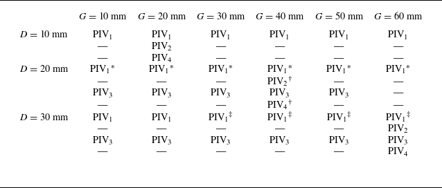
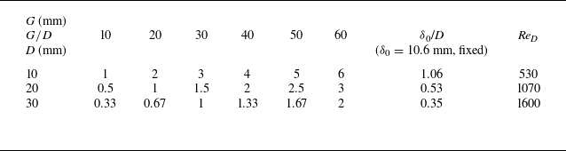

 δ0/D
 G/D
 G/D
 G/D
 G/D
 G/D
 G/D

 δ0/D

 δ0/D
 G/D

 δ0/D
 G/D
 G/D
 G/D
 G/D
 G/D
 G/D

 δ0/D
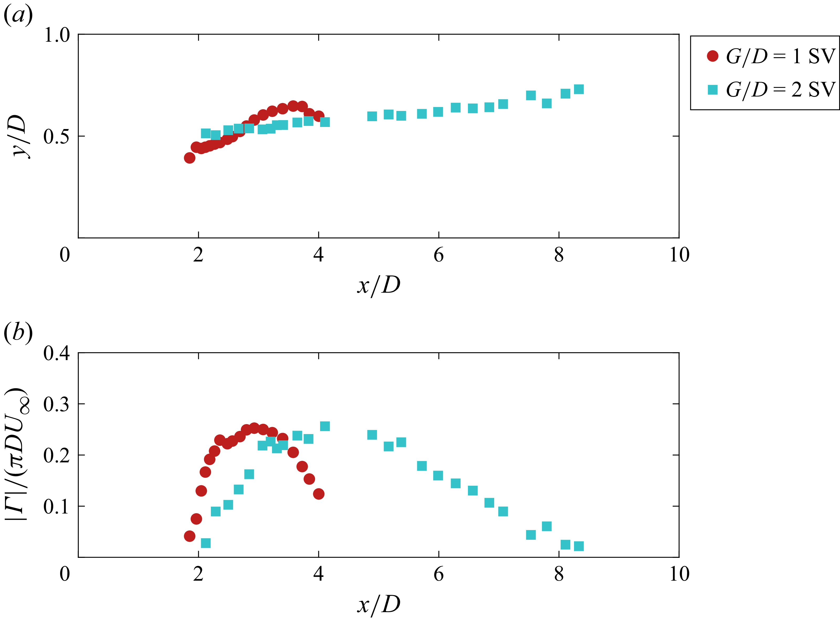
 δ0/D

 δ0/D
 G/D
 G/D
 G/D
 G/D
 G/D
 G/D

 δ0/D
 G/D
 G/D
 G/D
 G/D

 δ0/D
 G/D
 G/D
 G/D
 G/D
 G/D

 δ0/D

 δ0/D
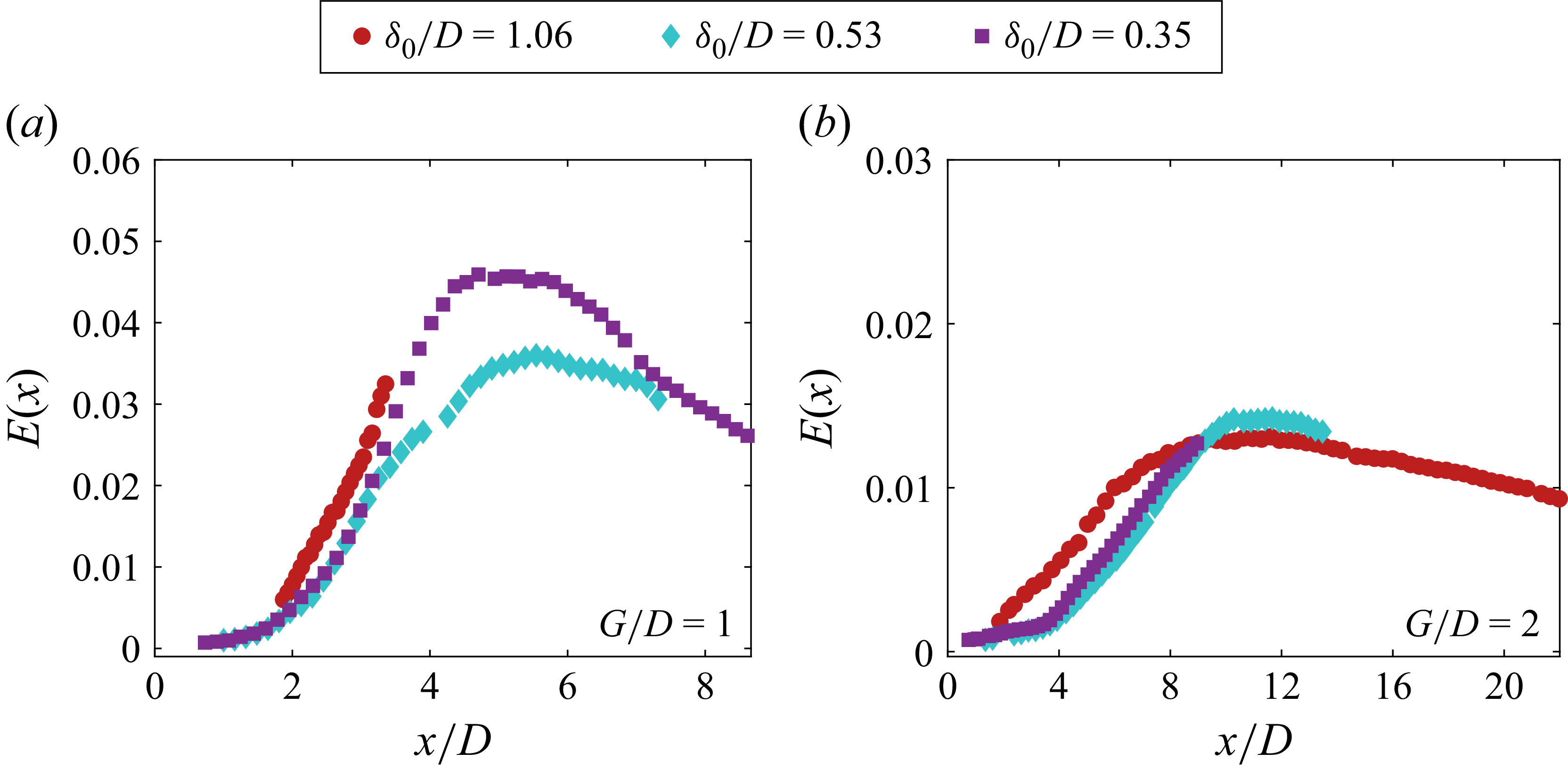
 G/D
 G/D
 G/D
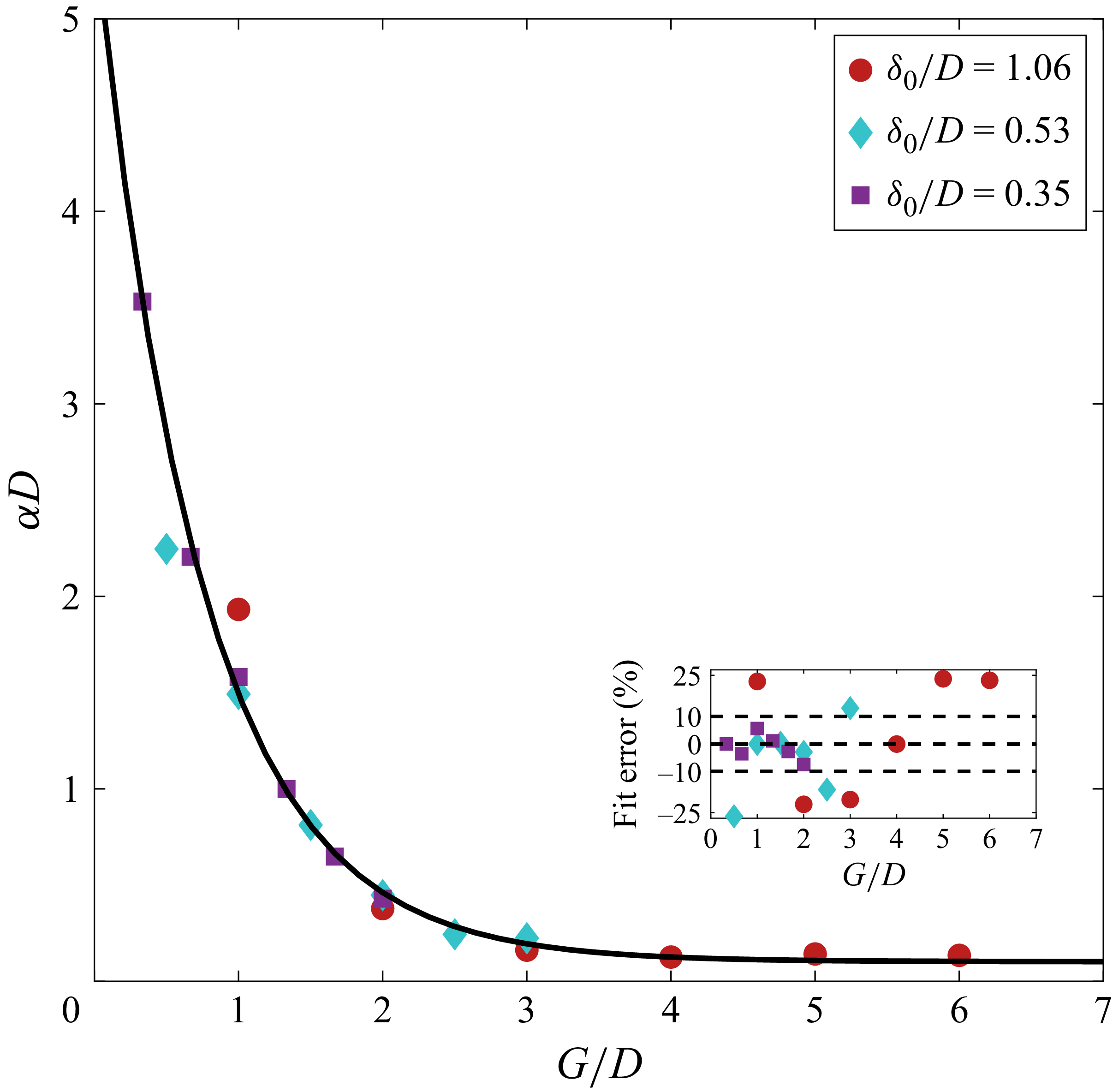
 G/D
 δ0/D
 G/D

 G/D

 G/D

 G/D
 δ0/D
 G/D
 G/D

 G/D

 G/D
 δ0/D

 G/D
 δ0/D

 G/D

 G/D
 δ0/D
 δ0/D

 G/D
 δ0/D
 δ0/D
 δ0/D

 G/D

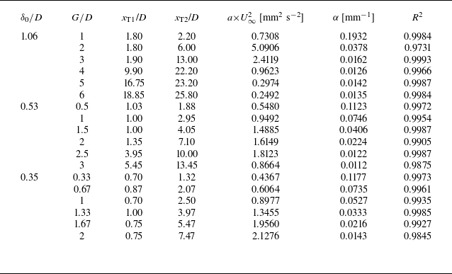
 U∞2
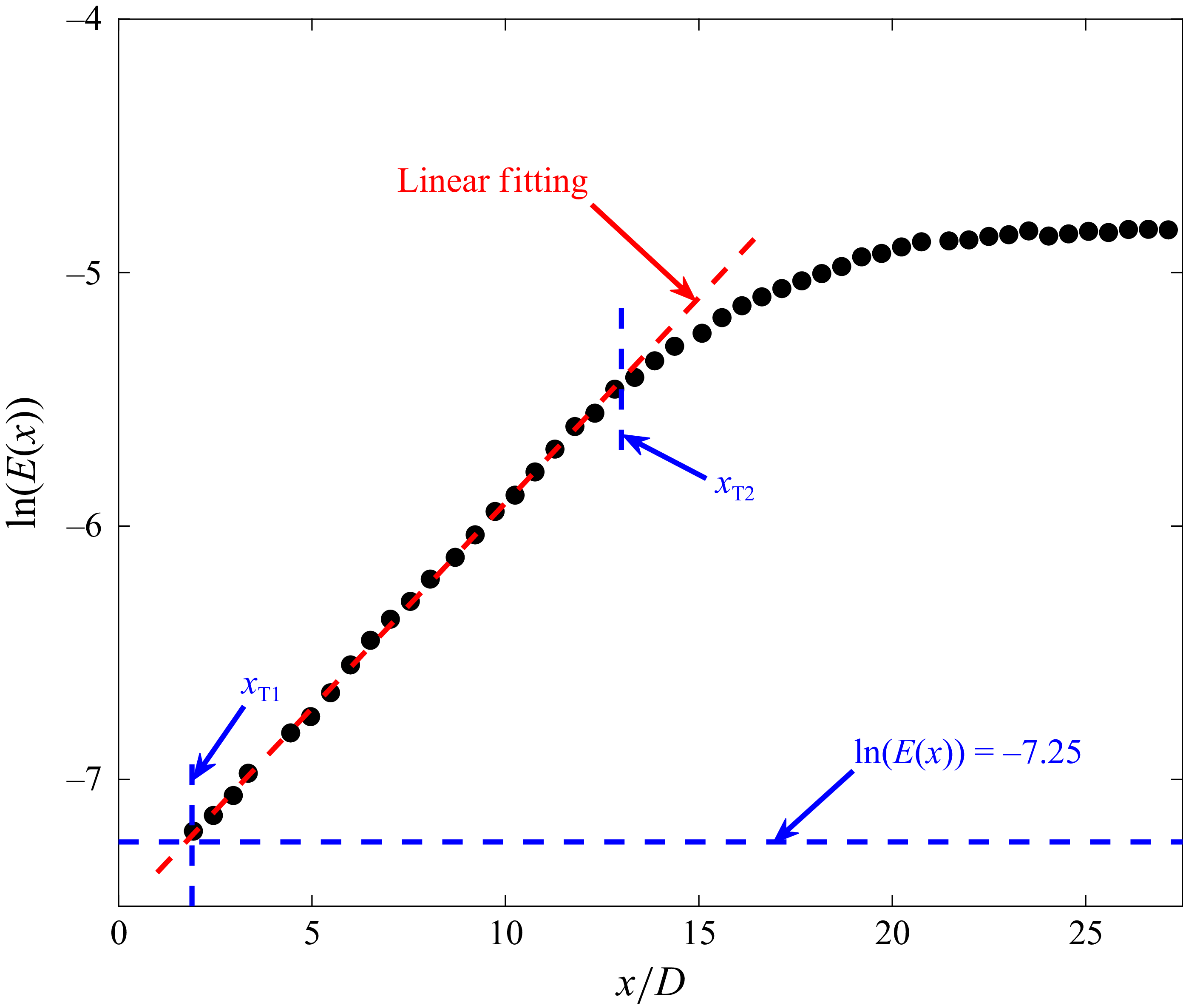
 G/D
 δ0/D

 δ0/D
 G/D
 G/D
 G/D
 G/D

 G/D
 δ0/D


