1 Introduction
Convection arises in many natural systems, from oceans and atmospheres to terrestrial mantles and liquid metal planetary cores. These systems often operate in dynamical regimes that cannot be attained in current laboratory experiments or numerical models. Significant effort has therefore focused on elucidating scaling relationships between the independent variables and diagnostics of the system behaviour. A particularly important diagnostic is the Nusselt number,
 $Nu$
, a global measure of the efficiency of heat transport in the convecting system. This study is motivated by convection in low viscosity liquid metal planetary cores where rotation and the spherical geometry significantly affect the dynamics and convection in the overlying silicate mantles sets the thermal boundary conditions at the top of core. Lateral variations in the temperature field at the bottom of silicate mantles can be very large relative to those expected in the metallic cores, resulting in correspondingly large lateral variations in the thermal boundary conditions imposed on the underlying core. We focus here on the impact of such heterogeneous boundary conditions on the heat transfer behaviour of rapidly rotating convection in spherical geometry.
1.1 Heat transport in convecting systems
The canonical system used to understand convective heat transfer is a conducting fluid sandwiched between two parallel plates oriented normal to the gravity vector, with an imposed temperature difference
 $\unicode[STIX]{x0394}T$
across the layer. The system is characterised by the Rayleigh number,
 $Ra$
, measuring the strength of the convective driving and the Prandtl number,
 $Pr=\unicode[STIX]{x1D708}/\unicode[STIX]{x1D705}$
, where
 $\unicode[STIX]{x1D708}$
is the kinematic viscosity and
 $\unicode[STIX]{x1D705}$
the thermal diffusivity. For a given value of
 $Pr$
, as
 $Ra$
is increased more heat is transported by advection and so
 $Nu=\unicode[STIX]{x1D716}Ra^{\unicode[STIX]{x1D6FE}}$
, with
 $\unicode[STIX]{x1D716},\unicode[STIX]{x1D6FE}>0$
. Malkus (Reference Malkus1954) assumed that
 $\unicode[STIX]{x0394}T$
is accommodated predominantly by conduction in two identical thermal boundary layers at the top and bottom of the system; by further assuming that the local Rayleigh number of the boundary layer equals the critical value for stability he found that
 $Nu\propto Ra^{1/3}$
. Numerical and physical experiments have produced a variety of scalings, which also depend on
 $Pr$
. Grossmann & Lohse (Reference Grossmann and Lohse2000) (see also Grossmann & Lohse Reference Grossmann and Lohse2001, Reference Grossmann and Lohse2002; Stevens et al.
Reference Stevens, van der Poel, Grossmann and Lohse2013) argued that these differences depend on whether the boundary layers or the bulk of the fluid dominate the kinematic and thermal dissipations, which divides
 $Ra$
–
 $Pr$
space into four regimes, each of which is divided into two subregimes based on the relative thickness of the thermal and kinetic boundary layers.
When the convecting system is rotating an additional non-dimensional parameter, the Ekman number,
 $E$
, quantifies the relative strength of the viscous and Coriolis forces. The Coriolis force has a stabilising effect on the convection such that the critical Rayleigh number for the onset of convection,
 $Ra_{C}$
, depends on
 $E$
. When convection is geostrophic, that is the first-order force balance is between the Coriolis force and pressure gradients, a heat transport scaling of
 $Nu\propto Ra^{3}E^{4}$
has been proposed (King, Stellmach & Aurnou Reference King, Stellmach and Aurnou2012) following the same reasoning as Malkus (Reference Malkus1954). However, in rapidly rotating systems a substantial interior temperature gradient can be maintained even to high
 $Ra$
(Sprague et al.
Reference Sprague, Julien, Knobloch and Werne2006; Julien et al.
Reference Julien, Rubio, Grooms and Knobloch2012b
; King, Stellmach & Buffett Reference King, Stellmach and Buffett2013; Gastine, Wicht & Aubert Reference Gastine, Wicht and Aubert2016; Julien et al.
Reference Julien, Aurnou, Calkins, Knobloch, Marti, Stellmach and Vasil2016), which enhances diffusive heat transport and alters
 $Nu$
relative to an equivalent non-rotating case. Experiments and numerical simulations in Cartesian geometry suggest that
 $\unicode[STIX]{x1D6FE}$
increases as
 $E$
decreases into the rotationally dominated regime (Stellmach et al.
Reference Stellmach, Lischper, Julien, Vasil, Cheng, Ribeiro, King and Aurnou2014; Cheng et al.
Reference Cheng, Stellmach, Ribeiro, Grannan, King and Aurnou2015). At
 $E=10^{-7}$
a value of
 $\unicode[STIX]{x1D6FE}=3.6$
has been found, with no indication that the scaling had yet reached an asymptotic limit with reducing
 $E$
(Cheng et al.
Reference Cheng, Stellmach, Ribeiro, Grannan, King and Aurnou2015). Reduced equations valid in the asymptotic limit of small
 $E$
(Sprague et al.
Reference Sprague, Julien, Knobloch and Werne2006) also find
 $\unicode[STIX]{x1D6FE}>3$
at low
 $E$
when the effect of Ekman pumping from no-slip boundary conditions is included (Stellmach et al.
Reference Stellmach, Lischper, Julien, Vasil, Cheng, Ribeiro, King and Aurnou2014; Aurnou et al.
Reference Aurnou, Calkins, Cheng, Julien, King, Nieves, Soderlund and Stellmach2015; Julien et al.
Reference Julien, Aurnou, Calkins, Knobloch, Marti, Stellmach and Vasil2016; Plumley et al.
Reference Plumley, Julien, Marti and Stellmach2016). Conversely, with free-slip boundary conditions the scaling at low-
 $E$
appears to saturate with
 $\unicode[STIX]{x1D6FE}=3/2$
, which is expected for a turbulent quasi-geostrophic regime where the heat transport is independent of both the thermal and viscous diffusivities (Gillet & Jones Reference Gillet and Jones2006; Julien et al.
Reference Julien, Knobloch, Rubio and Vasil2012a
; Stellmach et al.
Reference Stellmach, Lischper, Julien, Vasil, Cheng, Ribeiro, King and Aurnou2014).
In the spherical geometry considered in this paper, the boundary layer analysis is further complicated by asymmetric boundary layers, with the asymmetry in boundary layer thicknesses and temperature drops depending on both the radius ratio between the inner and outer boundaries and on the radial dependence of gravitational acceleration within the shell (Gastine, Wicht & Aurnou Reference Gastine, Wicht and Aurnou2015). In the absence of rotation the
 $Nu$
–
 $Ra$
scaling in the shell is similar to that of the plane layer (Gastine et al.
Reference Gastine, Wicht and Aurnou2015). At sufficiently high
 $Ra$
buoyancy forces will dominate Coriolis forces resulting in effectively non-rotating dynamics and
 $Nu$
–
 $Ra$
scaling. In the presence of rotation Gastine et al. (Reference Gastine, Wicht and Aubert2016) obtained the diffusivity-free scaling
 $Nu\propto Ra^{3/2}E^{2}$
in a small region of parameter space with
 $E\lesssim 10^{-6}$
and
 $RaE^{4/3}\simeq 10$
, conditions that placed the simulations in a dynamical regime that was both strongly nonlinear and dominated by rotation.
1.2 Heterogeneous boundary conditions for the core
Liquid metal planetary cores have higher thermal conductivity, and much lower viscosity, than their overlying solid silicate mantles. The resultant asymmetry in the thermal evolution of these systems implies that when considering thermal core–mantle interaction in simulations of core convection the use of fixed-flux boundary conditions would apply, whereas fixed-temperature boundary conditions would apply for the mantle (Olson Reference Olson2003, Reference Olson2016). Choosing fixed-temperature or fixed-flux boundary conditions results in different formulations of the Rayleigh and Nusselt numbers; these differences are outlined in § 2. However, after appropriate translation between the fixed-flux and fixed-temperature formulations the Nusselt–Rayleigh scaling is the same in both cases (Otero et al. Reference Otero, Wittenberg, Worthing and Doering2002; Ahlers, Grossmann & Lohse Reference Ahlers, Grossmann and Lohse2009; Johnston & Doering Reference Johnston and Doering2009; Calkins et al. Reference Calkins, Hale, Julien, Nieves, Driggs and Marti2015; Goluskin Reference Goluskin2015).
Mantle convection is much slower and supports much larger lateral variations in fluid properties (e.g. density, temperature, composition) than core convection (Olson Reference Olson2003, Reference Olson2016). It is therefore widely believed that convection in planetary cores must respond to a laterally varying pattern of heat flow imposed at the core–mantle boundary by mantle convection (Amit et al.
Reference Amit, Choblet, Olson, Monteux, Deschamps, Langlais and Tobie2015a
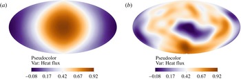
). For the present-day Earth, a pattern of heat flux (figure 1
b) is suggested by seismic tomography (e.g. Masters et al.
Reference Masters, Johnson, Laske and Bolton1996), which reveals two large low shear velocity provinces (LLSVPs) at the base of the mantle interpreted as hot, dense thermochemical piles in roughly antipodal locations beneath the Pacific Ocean and Africa (Garnero, McNamara & Shim Reference Garnero, McNamara and Shim2016). Seismically fast material between these LLSVPs is interpreted as the cold remnant of subducted lithospheric slabs. The largest component of this tomographic pattern is spherical harmonic of degree and order two (
 $Y_{2}^{2}$
), although other components also contribute. Inclusion of this pattern of heat flux in numerical models of the geodynamo can produce features in the spatial structure and temporal variation of the magnetic field similar to those observed for the Earth (Bloxham Reference Bloxham2000; Olson & Christensen Reference Olson and Christensen2002; Gubbins, Willis & Sreenivasan Reference Gubbins, Willis and Sreenivasan2007; Willis, Sreenivasan & Gubbins Reference Willis, Sreenivasan and Gubbins2007; Davies et al.
Reference Davies, Gubbins, Willis and Jimack2008; Amit, Aubert & Hulot Reference Amit, Aubert and Hulot2010; Amit, Deschamps & Choblet Reference Amit, Deschamps and Choblet2015b
; Olson Reference Olson2016).
The present-day Earth is but one example of the pattern, and amplitude, of core–mantle boundary heat-flux heterogeneity that can arise in planetary mantle convection. During the assembly of super-continents, a primarily hemispheric (
 $Y_{1}^{1}$
) pattern of mantle convection and hence core–mantle boundary heat flux (figure 1
a) may have existed (Zhong et al.
Reference Zhong, Zhang, Li and Roberts2007; Zhang & Zhong Reference Zhang and Zhong2011; Olson et al.
Reference Olson, Deguen, Hinnov and Zhong2013; Olson Reference Olson2016). A hemispheric heat-flux pattern has also been suggested for Mars to explain the Tharsis bulge (Zhong Reference Zhong2009; Šrámek & Zhong Reference Šrámek and Zhong2010), for the Moon to generate a non-axial magnetic field (Takahashi & Tsunakawa Reference Takahashi and Tsunakawa2009; Oliveira & Wieczorek Reference Oliveira and Wieczorek2017), and for hot tidally locked terrestrial exoplanets (Gelman, Elkins-Tanton & Seager Reference Gelman, Elkins-Tanton and Seager2011).
The amplitude of the lateral variations in the heat flux conducted through the outer boundary can be expressed as
 $$\begin{eqnarray}q_{L}^{\star }=\frac{q_{max}-q_{min}}{q_{ave}-q_{ad}},\end{eqnarray}$$
where
 $q_{max}$
,
 $q_{min}$
and
 $q_{ave}$
are the maximum, minimum and horizontally averaged heat flux through the boundary, respectively, and
 $q_{ad}$
is the heat flux conducted down the adiabatic gradient of the core at the boundary.
 $q_{L}^{\star }$
is challenging to precisely determine for Earth because it depends on the convective fluctuations as well as material properties of the mantle; it also will have varied through time. Estimates of the present-day total heat flow across the core–mantle boundary generally fall in the range
 $Q_{CMB}=5{-}20$
TW (Lay, Hernlund & Buffett Reference Lay, Hernlund and Buffett2008; Nimmo Reference Nimmo and Schubert2015; Kavner & Rainey Reference Kavner, Rainey, Terasaki and Fischer2016). Mantle convection simulations predict
 $(q_{max}-q_{min})/q_{ave}=O(1)$
for Earth (Nakagawa & Tackley Reference Nakagawa and Tackley2008; Olson et al.
Reference Olson, Deguen, Rudolph and Zhong2015). Recent upward revisions of the thermal conductivity of liquid iron mixtures increase
 $q_{ad}$
so that it is comparable to estimates of
 $q_{ave}$
(Lay et al.
Reference Lay, Hernlund and Buffett2008; Davies Reference Davies2015), in which case
 $q_{L}^{\star }\geqslant O(1)$
. The lateral variations that we include in our model all have zero mean, therefore values of
 $q_{L}^{\star }>2$
imply that for some portion of the outer boundary the heat flux is radially inward, although the integrated flux would remain outward. The average heat flux through the core–mantle boundary enters into the flux Rayleigh number for the core, for each flux Rayleigh number we will have a set of homogeneous and heterogeneous cases. Examples of the heat flux through the core–mantle boundary with
 $q_{L}^{\star }=2.3$
are shown in figure 1 for both hemispheric and tomographic perturbations to the mean.
Patterns of core–mantle boundary heat flux with hemispheric (a) and tomographic (b) perturbations added to the mean. The projection is centred on the negative
 $x$
-axis (the Pacific). In both cases
 $q_{L}^{\star }=2.3$
and the choice of normalisation results in a mean heat flux of approximately 0.42; note that only the deepest purples are associated with a negative (i.e. radially inward) heat flux.

Numerical (Zhang & Gubbins Reference Zhang and Gubbins1993, Reference Zhang and Gubbins1996; Gibbons, Gubbins & Zhang Reference Gibbons, Gubbins and Zhang2007; Davies, Gubbins & Jimack Reference Davies, Gubbins and Jimack2009; Dietrich, Hori & Wicht Reference Dietrich, Hori and Wicht2016) and physical (Sumita & Olson Reference Sumita and Olson1999, Reference Sumita and Olson2002) experiments have investigated rotating convection with laterally varying thermal boundary conditions for a variety of imposed patterns and
 $q_{L}^{\star }\ll 1$
up to
 $q_{L}^{\star }=O(1)$
. The previous numerical work, conducted predominantly at
 $Ra$
a few times critical, has shown that imposed boundary heterogeneity can have a substantial influence on the spatial patterns and time dependence of convection in the fluid shell, particularly when the wavelength of the imposed pattern is large. However, to our knowledge, the only previous study that compared heat transfer behaviour in rotating spherical shells with and without heterogeneous outer boundary forcing was that of Dietrich et al. (Reference Dietrich, Hori and Wicht2016) who carried out simulations of internally heated rotating spherical shell convection with a
 $Y_{1}^{1}$
outer boundary heat-flux pattern at
 $Pr=1$
and
 $E=2.5$
,
 $5\times 10^{-5}$
(using the definition of
 $E$
in § 2.1) and flux-based Rayleigh numbers up to 400 times critical for
 $E=5\times 10^{-5}$
. Estimating
 $\unicode[STIX]{x0394}T$
based on the maximum and minimum values of
 $T$
in the domain Dietrich et al. (Reference Dietrich, Hori and Wicht2016) found that
 $Nu$
is reduced by up to 50 % from the homogeneous case as the amplitude of heterogeneity is increased up to
 $q_{L}^{\star }=2$
(using our definition (1.1)).
Here we present results from 106 numerical simulations of bottom-heated rotating convection in a spherical shell with values of
 $E$
as low as
 $10^{-6}$
. We include two patterns of boundary heterogeneity and extend to flux-based Rayleigh numbers several hundred times critical. We focus in particular on heat transport within these models and the impact of the boundary heterogeneity on
 $Nu$
as a measure of convective efficiency. In § 2 we outline our theoretical basis for exploring heat transport in rotating convection; in § 3 we present summary results of all of our numerical simulations and more extended discussion of certain illustrative cases.
2 Theory
2.1 Governing equations and non-dimensionalisation
We employ a numerical model of convection of a homogeneous Boussinesq fluid confined within a rotating spherical shell (Willis et al.
Reference Willis, Sreenivasan and Gubbins2007). The fluid is characterised by its constant thermal diffusivity,
 $\unicode[STIX]{x1D705}$
, kinematic viscosity,
 $\unicode[STIX]{x1D708}$
, coefficient of thermal expansion,
 $\unicode[STIX]{x1D6FC}$
, and reference density,
 $\unicode[STIX]{x1D70C}_{0}$
. The thermal diffusivity can be expressed as
 $\unicode[STIX]{x1D705}=k/\unicode[STIX]{x1D70C}_{0}C_{P}$
, where
 $k$
is the thermal conductivity and
 $C_{P}$
the heat capacity of the fluid. The shell is defined in spherical coordinates,
 $(r,\unicode[STIX]{x1D703},\unicode[STIX]{x1D719})$
, by the inner and outer boundaries,
 $r_{i}$
and
 $r_{o}$
, respectively, and rotates with a constant angular velocity
 $\unicode[STIX]{x1D734}=\unicode[STIX]{x1D6FA}\hat{\boldsymbol{z}}$
. The governing equations for conservation of momentum, energy and mass can be written
 $$\begin{eqnarray}\displaystyle & \displaystyle \left(\frac{\unicode[STIX]{x2202}\boldsymbol{u}}{\unicode[STIX]{x2202}t}+(\boldsymbol{u}\boldsymbol{\cdot }\unicode[STIX]{x1D735})\boldsymbol{u}\right)+2\unicode[STIX]{x1D734}\times \boldsymbol{u}=-\frac{1}{\unicode[STIX]{x1D70C}_{0}}\unicode[STIX]{x1D735}\widetilde{P}+\frac{\unicode[STIX]{x1D70C}}{\unicode[STIX]{x1D70C}_{0}}\boldsymbol{g}+\unicode[STIX]{x1D708}\unicode[STIX]{x1D6FB}^{2}\boldsymbol{u}, & \displaystyle\end{eqnarray}$$
 $$\begin{eqnarray}\displaystyle & \displaystyle \frac{\unicode[STIX]{x2202}T}{\unicode[STIX]{x2202}t}+(\boldsymbol{u}\boldsymbol{\cdot }\unicode[STIX]{x1D735})T=\unicode[STIX]{x1D705}\unicode[STIX]{x1D6FB}^{2}T, & \displaystyle\end{eqnarray}$$
 $$\begin{eqnarray}\displaystyle & \displaystyle \unicode[STIX]{x1D735}\boldsymbol{\cdot }\boldsymbol{u}=0. & \displaystyle\end{eqnarray}$$
The modified pressure,
 $\widetilde{P}$
, includes the centrifugal potential. Gravity varies linearly with radius such that
 $\boldsymbol{g}=-(g_{o}/r_{o})\boldsymbol{r}$
, where
 $g_{o}$
is the gravitational acceleration at
 $r=r_{o}$
.
The fluid is incompressible (2.3) and so the velocity,
 $\boldsymbol{u}$
, can be decomposed into toroidal,
 ${\mathcal{T}}$
, and poloidal,
 ${\mathcal{P}}$
, components such that
 $$\begin{eqnarray}\boldsymbol{u}=\unicode[STIX]{x1D735}\times ({\mathcal{T}}\hat{\boldsymbol{r}})+\unicode[STIX]{x1D735}\times \unicode[STIX]{x1D735}\times ({\mathcal{P}}\hat{\boldsymbol{r}}).\end{eqnarray}$$
The toroidal and poloidal scalar fields can then be expressed in terms of spherical harmonics,
 $Y_{\ell }^{m}$
, with radially varying harmonic coefficients
 $\unicode[STIX]{x1D70F}_{\ell }^{m}(r)$
and
 $p_{\ell }^{m}(r)$
respectively. In this work we make use of the Schmidt semi-normalised spherical harmonics common in geomagnetic studies (e.g. Kono Reference Kono and Schubert2015). The boundary conditions on the velocity are non-penetrative and no slip such that
 $\boldsymbol{u}=0$
on
 $r=r_{i},r_{o}$
.
The temperature field,
 $T$
, can be written as
 $$\begin{eqnarray}T=T_{C}+T^{\prime },\end{eqnarray}$$
where
 $T_{C}$
is the steady-state temperature in the absence of flow and
 $T^{\prime }$
is the fluctuation about this state. We denote the coefficients of the spherical harmonic expansion of
 $T$
by
 $\unicode[STIX]{x1D717}_{\ell }^{m}(r)$
. Fixed-flux thermal boundary conditions are imposed such that
 $\unicode[STIX]{x1D735}T_{C}=-(\unicode[STIX]{x1D6FD}/r^{2})\hat{\boldsymbol{r}}$
at the inner and outer boundaries. Thus the total heat flow,
 $Q$
, is equal through the inner and outer surfaces and, for example, on the outer boundary
 $$\begin{eqnarray}Q=4\unicode[STIX]{x03C0}r_{o}^{2}q_{ave}=4\unicode[STIX]{x03C0}r_{o}^{2}(-k\unicode[STIX]{x1D735}T_{C})=4\unicode[STIX]{x03C0}k\unicode[STIX]{x1D6FD}.\end{eqnarray}$$
We introduce the following notation for radial, spherical surface and time averages, respectively
 $$\begin{eqnarray}\displaystyle & \displaystyle \{f(r)\}=\frac{1}{h}\int _{r_{i}}^{r_{o}}f(r)\,\text{d}r, & \displaystyle\end{eqnarray}$$
 $$\begin{eqnarray}\displaystyle & \displaystyle \langle f(r,\unicode[STIX]{x1D703},\unicode[STIX]{x1D719})\rangle =\frac{1}{4\unicode[STIX]{x03C0}r^{2}}\int _{0}^{\unicode[STIX]{x03C0}}\int _{0}^{2\unicode[STIX]{x03C0}}f(r,\unicode[STIX]{x1D703},\unicode[STIX]{x1D719})r^{2}\sin \unicode[STIX]{x1D703}\,\text{d}\unicode[STIX]{x1D719}\,\text{d}\unicode[STIX]{x1D703}, & \displaystyle\end{eqnarray}$$
 $$\begin{eqnarray}\displaystyle & \displaystyle \overline{f(t)}=\frac{1}{\unicode[STIX]{x1D70F}}\int _{t_{0}}^{t_{0}+\unicode[STIX]{x1D70F}}f(t)\,\text{d}t, & \displaystyle\end{eqnarray}$$
where
 $h=r_{o}-r_{i}$
is the shell thickness and
 $\unicode[STIX]{x1D70F}$
is the duration of the time averaging.
The control parameters that characterise the convecting system are derived from non-dimensionalisation of the governing equations (2.1)–(2.3). We scale length by the shell thickness,
 $h$
, time by the thermal diffusion time,
 $\unicode[STIX]{x1D70F}_{d}=h^{2}/\unicode[STIX]{x1D705}$
, and temperature by
 $\unicode[STIX]{x1D6FD}/h$
. With this choice of scaling the Ekman number, Prandtl number and modified Rayleigh number can be defined as
 $$\begin{eqnarray}E=\frac{\unicode[STIX]{x1D708}}{2\unicode[STIX]{x1D6FA}h^{2}},\quad Pr=\frac{\unicode[STIX]{x1D708}}{\unicode[STIX]{x1D705}},\quad \widetilde{Ra}=\frac{\unicode[STIX]{x1D6FC}g_{o}\unicode[STIX]{x1D6FD}}{2\unicode[STIX]{x1D6FA}\unicode[STIX]{x1D705}},\end{eqnarray}$$
and the resultant non-dimensional governing equations are
 $$\begin{eqnarray}\displaystyle & \displaystyle \frac{E}{Pr}\left(\frac{\unicode[STIX]{x2202}\boldsymbol{u}^{\star }}{\unicode[STIX]{x2202}t^{\star }}+(\boldsymbol{u}^{\star }\boldsymbol{\cdot }\unicode[STIX]{x1D735}^{\star })\boldsymbol{u}^{\star }\right)+\hat{\boldsymbol{z}}\times \boldsymbol{u}^{\star }=-\unicode[STIX]{x1D735}^{\star }\widetilde{P^{\star }}+\widetilde{Ra}T^{\prime \star }\boldsymbol{r}^{\star }+E\unicode[STIX]{x1D6FB}^{\star 2}\boldsymbol{u}^{\star }, & \displaystyle\end{eqnarray}$$
 $$\begin{eqnarray}\displaystyle & \displaystyle \frac{\unicode[STIX]{x2202}T^{\star }}{\unicode[STIX]{x2202}t^{\star }}+(\boldsymbol{u}^{\star }\boldsymbol{\cdot }\unicode[STIX]{x1D735}^{\star })T^{\star }=\unicode[STIX]{x1D6FB}^{\star 2}T^{\star }, & \displaystyle\end{eqnarray}$$
 $$\begin{eqnarray}\displaystyle & \displaystyle \unicode[STIX]{x1D735}^{\star }\boldsymbol{\cdot }\boldsymbol{u}^{\star }=0. & \displaystyle\end{eqnarray}$$
In all of our models
 $Pr=1$
and the radius ratio of the shell is set to
 $r_{i}/r_{o}=0.35$
, the value for Earth’s core. The modified Rayleigh number is related to a flux Rayleigh number by
 $$\begin{eqnarray}Ra_{F}=\frac{\unicode[STIX]{x1D6FC}g_{o}\unicode[STIX]{x1D6FD}h^{2}}{\unicode[STIX]{x1D708}\unicode[STIX]{x1D705}}=\frac{\widetilde{Ra}}{E}.\end{eqnarray}$$
To convert from flux-based to temperature-based Rayleigh number we need to relate
 $\unicode[STIX]{x1D6FD}$
to the temperature drop across the convecting system,
 $\unicode[STIX]{x0394}T$
. The solution to the spherical shell conduction problem (see (2.22)–(2.25) below) gives
 $\unicode[STIX]{x1D6FD}=\unicode[STIX]{x0394}T_{C}r_{i}r_{o}/h$
, which in combination with our expression for the Nusselt number ((2.30) below) leads to
 $$\begin{eqnarray}Ra_{T}=\frac{\unicode[STIX]{x1D6FC}g_{o}\unicode[STIX]{x0394}Th^{3}}{\unicode[STIX]{x1D708}\unicode[STIX]{x1D705}}=\frac{Ra_{F}}{Nu}\frac{h^{2}}{r_{i}r_{o}},\end{eqnarray}$$
where
 $\unicode[STIX]{x0394}T$
is taken to be
 $\overline{\unicode[STIX]{x0394}\langle T\rangle }$
, the measured time-averaged temperature drop across the convecting system.
Below we will generally present results relative to the advection time scale,
 $\unicode[STIX]{x1D70F}_{a}=h/U$
, where
 $U$
is a characteristic velocity for the flow. The ratio between thermal diffusion and advection time scales is the thermal Péclet number,
 $Pe=\unicode[STIX]{x1D70F}_{d}/\unicode[STIX]{x1D70F}_{a}=Uh/\unicode[STIX]{x1D705}$
. The thermal Péclet number is the product of the Prandtl and Reynolds numbers; since we set
 $Pr=1$
in all of our models we have
 $Pe=Re=Uh/\unicode[STIX]{x1D708}$
. The characteristic velocity is derived from the kinetic energy and after non-dimensionalisation we have
 $$\begin{eqnarray}Pe=Re=U^{\star }=\sqrt{\frac{2KE^{\star }}{Vs^{\star }}},\end{eqnarray}$$
where
 $Vs^{\star }$
is the non-dimensional volume of the domain and
 $KE^{\star }$
is the non-dimensional kinetic energy of the system defined by
 $$\begin{eqnarray}KE^{\star }={\textstyle \frac{1}{2}}\iiint _{Vs^{\star }}\overline{\boldsymbol{u}^{\star ^{2}}}\,\text{d}V^{\star }.\end{eqnarray}$$
2.2 Heat transport
The Nusselt number provides a global measure of the efficiency of heat transport in a convecting system by comparing the total heat flux through the system to that which could be transferred by conduction alone. Equation (2.2) can be written as
 $$\begin{eqnarray}\unicode[STIX]{x1D70C}_{0}C_{P}\frac{\unicode[STIX]{x2202}T}{\unicode[STIX]{x2202}t}+\unicode[STIX]{x1D735}\boldsymbol{\cdot }\boldsymbol{q}=0,\end{eqnarray}$$
where the total heat flux
 $$\begin{eqnarray}\boldsymbol{q}=\unicode[STIX]{x1D70C}_{0}C_{P}\boldsymbol{u}T-k\unicode[STIX]{x1D735}T\end{eqnarray}$$
is the sum of the advective and diffusive contributions.
We first revisit the canonical example of a plane layer of thickness of
 $d$
and fixed temperature difference across the layer of
 $\unicode[STIX]{x0394}T$
. In this case the Nusselt number is
 $$\begin{eqnarray}Nu=\frac{\langle \overline{\boldsymbol{q}}\boldsymbol{\cdot }\hat{\boldsymbol{z}}\rangle }{k\unicode[STIX]{x0394}T/d},\end{eqnarray}$$
where the total vertical heat flux,
 $\boldsymbol{q}\boldsymbol{\cdot }\hat{\boldsymbol{z}}$
, can be averaged over any horizontal surface and the conduction solution gives
 $(\unicode[STIX]{x1D735}T_{C})\boldsymbol{\cdot }\hat{\boldsymbol{z}}=-\unicode[STIX]{x0394}T/d$
. It can be particularly useful to consider the top or bottom surface, where
 $\boldsymbol{q}\boldsymbol{\cdot }\hat{\boldsymbol{z}}$
is purely conductive, such that the Nusselt number can be written
 $$\begin{eqnarray}Nu=\frac{-\langle (\unicode[STIX]{x1D735}\overline{T})\boldsymbol{\cdot }\hat{\boldsymbol{n}}\rangle |_{top}}{-(\unicode[STIX]{x1D735}T_{C})\boldsymbol{\cdot }\hat{\boldsymbol{n}}|_{top}}=\frac{\langle (\unicode[STIX]{x1D735}\overline{T})\boldsymbol{\cdot }\hat{\boldsymbol{n}}\rangle |_{bottom}}{(\unicode[STIX]{x1D735}T_{C})\boldsymbol{\cdot }\hat{\boldsymbol{n}}|_{bottom}},\end{eqnarray}$$
where
 $\hat{\boldsymbol{n}}$
is the outward normal with respect to the domain.
In numerical or physical experiments with fixed-temperature boundary conditions the Nusselt number can thus be evaluated by determining
 $\langle \overline{\boldsymbol{q}}\boldsymbol{\cdot }\hat{\boldsymbol{n}}\rangle$
for a sufficiently large averaging time. Fixed-flux boundary conditions set
 $\unicode[STIX]{x1D735}T=\unicode[STIX]{x1D735}T_{C}$
on both boundaries at every instant in time, in which case (2.21) suggests
 $Nu=1$
regardless of convective vigour. Although the non-penetration condition requires that all heat is transferred by conduction across the boundaries, within the fluid interior the advective heat transport will reduce the temperature gradient. In experiments where
 $\langle \overline{\boldsymbol{q}}\boldsymbol{\cdot }\hat{\boldsymbol{n}}\rangle$
is fixed, the temperature drop across the system is the quantity to be determined in (2.20).
In our model, with fixed-flux boundaries and spherical shell geometry, the conduction problem is
 $$\begin{eqnarray}\frac{\unicode[STIX]{x1D705}}{r^{2}}\frac{\text{d}}{\text{d}r}\left(r^{2}\frac{\text{d}T_{C}}{\text{d}r}\right)=0,\end{eqnarray}$$
subject to boundary conditions
 $$\begin{eqnarray}\left.\frac{\text{d}T_{C}}{\text{d}r}\right|_{r=r_{o}}=-\frac{\unicode[STIX]{x1D6FD}}{r_{o}^{2}},\quad \left.\frac{\text{d}T_{C}}{\text{d}r}\right|_{r=r_{i}}=-\frac{\unicode[STIX]{x1D6FD}}{r_{i}^{2}}.\end{eqnarray}$$
The solution is
 $$\begin{eqnarray}\frac{\text{d}T_{C}}{\text{d}r}=-\frac{\unicode[STIX]{x1D6FD}}{r^{2}},\quad T_{C}=\frac{\unicode[STIX]{x1D6FD}}{r}+B,\end{eqnarray}$$
where
 $B$
is a constant of integration that is not constrained by the flux boundary conditions. Therefore, the temperature drop across the shell in the conduction only case is
 $$\begin{eqnarray}\unicode[STIX]{x0394}T_{C}=\unicode[STIX]{x1D6FD}\left(\frac{1}{r_{i}}-\frac{1}{r_{o}}\right)=\frac{\unicode[STIX]{x1D6FD}h}{r_{i}r_{o}}.\end{eqnarray}$$
The total heat flux of the convecting system is found by time averaging equation (2.18) for a duration that is sufficiently long to reach a statistical steady state, in which case
 $\unicode[STIX]{x1D735}\boldsymbol{\cdot }\overline{\boldsymbol{q}}=0$
within the domain, a consequence of the absence of internal heat sources. It follows that
 $$\begin{eqnarray}\iiint _{Vs}\unicode[STIX]{x1D735}\boldsymbol{\cdot }\overline{\boldsymbol{q}}\,\text{d}V=0=\oint \overline{\boldsymbol{q}}\boldsymbol{\cdot }\hat{\boldsymbol{n}}\,\text{d}S=4\unicode[STIX]{x03C0}\mathop{r}_{o}^{2}\langle \overline{\boldsymbol{q}}\boldsymbol{\cdot }\hat{\boldsymbol{r}}\rangle |_{r=r_{o}}-4\unicode[STIX]{x03C0}r_{i}^{2}\langle \overline{\boldsymbol{q}}\boldsymbol{\cdot }\hat{\boldsymbol{r}}\rangle |_{r=r_{i}}\end{eqnarray}$$
and, since the volume of integration is arbitrary,
 $4\unicode[STIX]{x03C0}r^{2}\langle \overline{\boldsymbol{q}}\boldsymbol{\cdot }\hat{\boldsymbol{r}}\rangle$
is independent of
 $r$
. The imposed boundary conditions require
 $u_{r}|_{r=r_{i}}=u_{r}|_{r=r_{o}}=0$
,
 $\unicode[STIX]{x2202}\overline{T}/\unicode[STIX]{x2202}r|_{r=r_{o}}=-\unicode[STIX]{x1D6FD}/r_{o}^{2}$
, and
 $\unicode[STIX]{x2202}\overline{T}/\unicode[STIX]{x2202}r|_{r=r_{i}}=-\unicode[STIX]{x1D6FD}/r_{i}^{2}$
, therefore
 $$\begin{eqnarray}4\unicode[STIX]{x03C0}r^{2}\langle \overline{\boldsymbol{q}}\boldsymbol{\cdot }\hat{\boldsymbol{r}}\rangle =4\unicode[STIX]{x03C0}r_{o}^{2}\langle -k\unicode[STIX]{x2202}\overline{T}/\unicode[STIX]{x2202}r\rangle |_{r=r_{o}}=4\unicode[STIX]{x03C0}r_{i}^{2}\langle -k\unicode[STIX]{x2202}\overline{T}/\unicode[STIX]{x2202}r\rangle |_{r=r_{i}}=4\unicode[STIX]{x03C0}k\unicode[STIX]{x1D6FD}\end{eqnarray}$$
and
 $$\begin{eqnarray}\langle \overline{\boldsymbol{q}}\boldsymbol{\cdot }\hat{\boldsymbol{r}}\rangle =k\unicode[STIX]{x1D6FD}/r^{2}=-k(\text{d}T_{C}/\text{d}r).\end{eqnarray}$$
Although
 $4\unicode[STIX]{x03C0}r^{2}\langle \overline{\boldsymbol{q}}\boldsymbol{\cdot }\hat{\boldsymbol{r}}\rangle$
is independent of
 $r$
, the advective and diffusive contributions to the total radial heat flux will vary. The global balance between the advective and diffusive contributions requires integration with respect to
 $r$
, leading to the following expression for the Nusselt number based on fluxes
 $$\begin{eqnarray}Nu_{F}=\frac{\{\langle \overline{\boldsymbol{q}}\boldsymbol{\cdot }\hat{\boldsymbol{r}}\rangle \}}{\{\langle -k\unicode[STIX]{x2202}\overline{T}/\unicode[STIX]{x2202}r\rangle \}}.\end{eqnarray}$$
Using (2.28) allows us to recast
 $Nu_{F}$
as
 $$\begin{eqnarray}\frac{-{\displaystyle \frac{k}{h}}\displaystyle \int (\text{d}T_{C}/\text{d}r)\,\text{d}r}{-{\displaystyle \frac{k}{h}}\displaystyle \int (\text{d}\langle \overline{T}\rangle /\text{d}r)\,\text{d}r}=\frac{\unicode[STIX]{x0394}T_{C}}{\unicode[STIX]{x0394}\langle \overline{T}\rangle }=Nu_{T}.\end{eqnarray}$$
The order of the horizontal and temporal averaging in
 $\unicode[STIX]{x0394}\langle \overline{T}\rangle$
is interchangeable and in practice we determine
 $\overline{\unicode[STIX]{x0394}\langle T\rangle }$
. Note that when considering the non-dimensional form of (2.30) our geometry and choice of temperature scaling results in
 $\unicode[STIX]{x0394}T_{C}^{\star }\approx 1.2$
rather than unity, as would be typical for Cartesian geometry (e.g. Otero et al.
Reference Otero, Wittenberg, Worthing and Doering2002; Goluskin Reference Goluskin2015) (see also appendix A).
Let us consider the implications of a change in Nusselt number between two models with the same value of
 $Ra_{F}$
but different patterns or amplitudes of boundary heat-flux variation. Equation (2.30) shows that a change in
 $Nu$
corresponds to a change in the temperature drop across the system since
 $\unicode[STIX]{x0394}T_{C}$
is set by
 $\unicode[STIX]{x1D6FD}$
(recall (2.25)), and hence by
 $Ra_{F}$
. Furthermore, equations (2.19) and (2.28) imply that any change in
 $\langle \unicode[STIX]{x2202}\overline{T}/\unicode[STIX]{x2202}r\rangle$
must be compensated by a complementary change in
 $\langle \overline{u_{r}T}\rangle$
. Changing the efficiency of heat transport requires alteration of both the temperature and velocity fields.
The time-averaged temperature drop across the system can be expressed using the spherical harmonic expansion of the temperature field as
 $$\begin{eqnarray}\unicode[STIX]{x0394}\langle \overline{T}\rangle =\overline{\unicode[STIX]{x1D717}_{0}^{0}(r_{i})}-\overline{\unicode[STIX]{x1D717}_{0}^{0}(r_{o})};\end{eqnarray}$$
any change in
 $Nu_{T}$
induced by the heterogeneous boundary condition must influence the
 $Y_{0}^{0}$
spherical harmonic component of the temperature field. The imposed patterns of boundary heterogeneity have zero mean and hence the homogeneous and heterogeneous thermal boundary conditions have identical
 $Y_{0}^{0}$
components for a given
 $Ra_{F}$
. Since there is no interaction between harmonics in the diffusive part of the energy equation (2.2), any change in
 $\overline{\unicode[STIX]{x0394}T}$
, and hence
 $\unicode[STIX]{x1D717}_{0}^{0}(r)$
, must arise from nonlinear interaction between the flow and temperature fields. This can be seen by writing equation (2.28) as
 $$\begin{eqnarray}\overline{\langle u_{r}T\rangle }=\unicode[STIX]{x1D705}\frac{\text{d}}{\text{d}r}\left(\overline{\unicode[STIX]{x1D717}_{0}^{0}}-T_{C}\right).\end{eqnarray}$$
The radial component of velocity depends only on the poloidal component of the velocity field, thus spherical harmonic expansion of the variables on the left-hand side of (2.32) leads to
 $$\begin{eqnarray}\frac{1}{r}\mathop{\sum }_{\ell ,m}\left(\frac{\ell (\ell +1)}{2\ell +1}\right)\overline{p_{\ell }^{m}\unicode[STIX]{x1D717}_{\ell }^{m}}=\unicode[STIX]{x1D705}\frac{\text{d}}{\text{d}r}\left(\overline{\unicode[STIX]{x1D717}_{0}^{0}}-T_{C}\right),\end{eqnarray}$$
where we have made use of the orthogonality of the (Schmidt-normalised) spherical harmonics. Equation (2.3) implies that
 $p_{0}^{0}=0$
and thus we see that
 $\unicode[STIX]{x1D717}_{0}^{0}$
must be modified by interactions between flow and temperature at other harmonics.
Consider, for example, a homogeneous model to which is added a
 $Y_{1}^{1}$
heat-flux heterogeneity at the outer boundary. In this case we anticipate that the heat-flux heterogeneity will increase
 $\overline{\unicode[STIX]{x1D717}_{1}^{1}}$
near the top of the fluid core, relative to the homogeneous boundary case. This temperature perturbation in the core then generates, on average, some amount of
 $p_{1}^{1}$
flow by promoting (inhibiting) downwelling in regions of enhanced (reduced) outward heat flux across the boundary. Any resultant increased correlation between the hemispheric patterns in radial flow and temperature (i.e. an increase in
 $\overline{p_{1}^{1}\unicode[STIX]{x1D717}_{1}^{1}}$
for radii near
 $r_{o}$
) implies an altered
 $\text{d}\overline{\unicode[STIX]{x1D717}_{0}^{0}}/\text{d}r$
and hence
 $Nu_{T}$
. Correlations at harmonics other than those of the imposed heterogeneity could also be promoted by the boundary heterogeneity through some more complex set of dynamics. Regardless, for fixed
 $Ra_{F}$
the total heat transport through the system remains unchanged and an increase in
 $Nu$
with heterogeneous boundary conditions, which reflects a repartitioning of heat transport from conduction to advection, requires an increased correlation between
 $u_{r}$
and
 $T$
and a smaller average radial temperature gradient. This reorganisation of flow and temperature fields could occur throughout the domain or be limited to a relatively restricted region, for example near the outer boundary. In the following section we present the heat transport results for our suite of models. We will not present a detailed analysis of the association between flow and
 $Nu$
for all simulations, but any case for which the heterogeneous boundary conditions have altered
 $Nu$
relative to the equivalent homogeneous case must have some reorganisation of the time-averaged flow in accordance with the principles outlined here.
3 Results and discussion
3.1 Numerical model, parameters and convergence tests
The pseudo-spectral method used in this work is described in Willis et al. (Reference Willis, Sreenivasan and Gubbins2007); it passes the dynamo benchmark and performs comparably to other pseudo-spectral methods (Matsui et al.
Reference Matsui, Heien, Aubert, Aurnou, Avery, Brown, Buffett, Busse, Christensen and Davies2016). The velocity field is decomposed into toroidal and poloidal scalars, which ensures that the divergence-free condition is satisfied exactly. All scalars are then expanded in Schmidt-normalised spherical harmonics on each spherical surface and represented in radius by second-order finite differences. The finite difference points are located at the zeros of the Chebyshev polynomials, providing finer spacing near the upper and lower boundaries. Time stepping is accomplished in spectral space using a predictor–corrector scheme that treats diffusion terms implicitly, while the Coriolis, buoyancy and nonlinear terms are treated explicitly. Nonlinear terms are transformed into real space at each time step using the spherical transform method (Orszag Reference Orszag1971). At each radius multiplications are performed on a Gauss–Legendre grid with
 $(3/2)\ell _{max}$
colatitude points and
 $3\ell _{max}$
longitude points. The number of radial grid points,
 $N_{r}$
, and the maximum spherical harmonic degree and order,
 $\ell _{max}=m_{max}$
, for all runs are given in appendix B. Our choices of
 $\ell _{max}$
are similar to those used by Gastine et al. (Reference Gastine, Wicht and Aubert2016) for comparable control parameters.
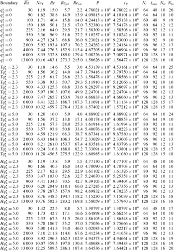
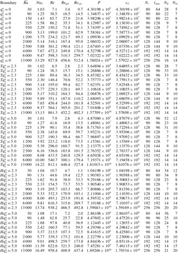
In this work we focus on the global heat transport of rotating convection in a spherical shell with variable heat-flux boundary conditions. To do so we have run a suite of 106 numerical simulations with: Ekman number,
 $E=10^{-4}$
,
 $10^{-5}$
,
 $10^{-6}$
; flux Rayleigh number,
 $3\times 10^{5}\leqslant Ra_{F}\leqslant 1.8\times 10^{10}$
; Prandtl number,
 $Pr=1$
. Strong rotation inhibits the onset of convection; for our thermal and mechanical boundary conditions, and choices of Ekman and Prandtl numbers, linear stability analysis of the homogeneous cases (for details see Gibbons et al.
Reference Gibbons, Gubbins and Zhang2007; Davies et al.
Reference Davies, Gubbins and Jimack2009) indicates that our simulations fall in the range
 $1.2Ra_{C}\lesssim Ra_{F}\lesssim 800Ra_{C}$
(the critical Rayleigh number,
 $\widetilde{Ra}_{C}$
, and most unstable mode at onset,
 $m_{C}$
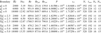
, for our cases are given in table 1). The control and output parameters for all runs are detailed in appendix B.
Critical Rayleigh number and critical azimuthal wavenumber for our simulations.

We consider three different patterns of heat flux imposed at the outer boundary. Simulations with a homogeneous outer boundary have
 $q_{L}^{\star }=0$
. Cases with the hemispheric pattern described by the
 $Y_{1}^{1}$
spherical harmonic (figure 1
a) are referred to using
 $Hq_{L}^{\star }$
, in these simulations
 $q_{max}$
(
 $q_{min}$
) is aligned with the negative (positive)
 $x$
axis. Cases with boundary heterogeneity derived from the observed pattern of seismic velocity variations in the lowermost mantle (Masters et al.
Reference Masters, Johnson, Laske and Bolton1996) (figure 1
b) are referred to using
 $Tq_{L}^{\star }$
. The amplitude of the heat-flux heterogeneity is set to
 $Hq_{L}^{\star },Tq_{L}^{\star }=2.3$
or 5.0; values based on a proposed scaling from seismic velocity to temperature following the work of Nakagawa & Tackley (Reference Nakagawa and Tackley2008).
(a) Convergence of all models as measured by the difference between the time average of the buoyancy production,
 $P$
, and viscous dissiaption,
 $\unicode[STIX]{x1D716}_{U}$
, both integrated over the volume of the shell. (b) Convergence of the time-averaged Nusselt number for all models as measured by the difference between
 $\overline{Nu_{F}}$
and
 $\overline{Nu_{T}}$
. Symbol shapes indicate the value of
 $E$
, symbol size and colour indicate the nature of the boundary conditions.

The spatial convergence of each simulation is evaluated by checking that the buoyancy production throughout the volume,
 $P$
, is matched by the viscous dissipation,
 $\unicode[STIX]{x1D716}_{U}$
, in the time average (see e.g. Gastine et al.
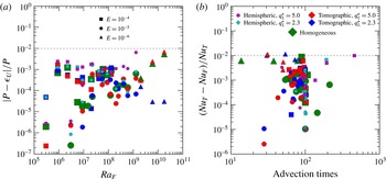
Reference Gastine, Wicht and Aurnou2015). Figure 2(a) shows
 $|P-\unicode[STIX]{x1D716}_{U}|/P$
for all cases, this residual is always less than
 $10^{-2}$
. We compute the thickness of the viscous boundary layers at
 $r=r_{i},r_{o}$
based on the location of the local maxima in the radial profile of horizontal velocity variations following the method described in King et al. (Reference King, Stellmach and Buffett2013) and report the number of grid points within the boundary layers for each simulation in appendix B. With one exception, there are at least 7 points in both boundary layers and the majority of simulations have many more points than this (the lowest Rayleigh homogeneous model at
 $E=10^{-5}$
has 28 radial grid points within the boundary layer near
 $r_{i}$
, but only 5 within the boundary layer near
 $r_{o}$
). These boundary layer resolutions are comparable to those used by Stevens, Verzicco & Lohse (Reference Stevens, Verzicco and Lohse2010) for resolving the radial structure of thermal boundary layers in Rayleigh–Bénard convection.
After removal of the initial transient, time averages are constructed over a span of at least 10 advection times and in general of around 100 advection times. The Reynolds number allows conversion from advection to diffusion times; the durations of the runs mostly lie between 0.01 and 10 diffusion times. Convergence of the Nusselt number is tested by considering the difference between
 $\overline{Nu_{F}}$
and
 $\overline{Nu_{T}}$
as determined by time averaging over the run. As shown in figure 2(b) the difference between these two methods of calculating the Nusselt number is of the order of 1 % or less.
The case with
 $E=10^{-4}$
,
 $Ra_{F}=2.25\times 10^{6}$
and
 $Hq_{L}^{\star }=5.0$
(the rightmost point in figure 2
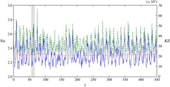
b) required over 450 advection times to reach our 1 % convergence target, significantly longer than the other runs. The kinetic energy and instantaneous
 $Nu$
time series for this case display large amplitude fluctuations (figure 3). The system switches between two states each of which persists for several advection times, with times of higher (lower)
 $KE^{\star }$
correlated with periods of higher (lower)
 $Nu$
;
 $Re=67.3$
for this run, so the period of the oscillations is approximately 0.1 diffusion times. There is a time lag between the total and zonal kinetic energies of the system suggesting that the convection generates progressively stronger zonal flow until the resultant shear disrupts the convective rolls. Similar relaxation oscillations have been seen in homogeneous rotating spheres (see e.g. Busse Reference Busse2002, for a review), here the boundary heterogeneity modulates convection activity such that localised convection is concentrated in the hemisphere that is most strongly cooled by the overlying mantle.
 $KE^{\star }$
(dash-dot green line, right-hand axis),
 $Nu_{T}$
(blue solid line, left-hand axis), and the running average of
 $Nu_{T}$
(dotted red line, left-hand axis) for the run with
 $E=10^{-4}$
,
 $Ra_{F}=2.25\times 10^{6}$
and
 $Hq_{L}^{\star }=5.0$
. The representative flow patterns for the low- and high-
 $Nu$
states shown in figure 4 were found by averaging over the time periods indicated by the grey shading. Time is measured by the advection time scale.

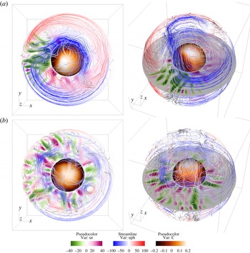
Time-averaged flows for the run with
 $E=10^{-4}$
,
 $Ra_{F}=2.25\times 10^{6}$
, and
 $Hq_{L}^{\star }=5.0$
averaged over a period of high
 $Nu$
(a) and a period of low
 $Nu$
(b), the averaging periods are indicated by the grey bands in figure 3. The equatorial plane is coloured by
 $u_{r}^{\star }$
in the plane (green–magenta), streamlines of the time-averaged velocity field are coloured by
 $u_{\unicode[STIX]{x1D719}}^{\star }$
(blue–red), and the inner boundary is coloured by temperature anomaly relative to the horizontal average (brown–orange–white). On the outer boundary
 $q_{min}$
is aligned with the positive
 $x$
-axis and
 $q_{max}$
is aligned with the negative
 $x$
-axis. The rotation vector points in the positive
 $z$
direction.

Representative flow patterns for the low- and high-
 $Nu$
states were found by averaging over the time periods indicated by the grey shading in figure 3, each of which corresponds to approximately three advection times. The flow pattern in the low-
 $Nu$
state (figure 4
b) consists of a well-developed zonal flow in the shell interior interacting with convective rolls aligned with the rotation axis. Relatively hot fluid accumulates near the outer boundary in the positive
 $x$
hemisphere below
 $q_{min}$
, which tends to suppress the formation of convective rolls, and hence radial flow, above mid-depth in that hemisphere. Conversely,
 $q_{max}$
in the negative
 $x$
hemisphere tends to enhance radial flow. The high-
 $Nu$
state (figure 4
a) is characterised by two large-scale circulations anchored by a large downwelling beneath
 $q_{max}$
. Peak upwelling velocities in the high-
 $Nu$
state are similar to those of the low-
 $Nu$
state; however, peak downwelling velocities have approximately 50 % greater amplitude. The strong downwelling is relatively effective at transporting cold material deep within the shell such that the high-
 $Nu$
state has a long-wavelength azimuthal temperature anomaly at the equator of the inner boundary, in addition to the general pattern of positive (negative) temperature anomalies at high (low) latitudes seen at all times in this model. The higher average velocities and changed pattern of convection increase the global correlation between radial velocity and temperature and correspondingly reduce the average temperature drop across the shell during the high-
 $KE^{\star }$
–high-
 $Nu$
state.
Scaling of
 $Nu_{T}$
against
 $Ra_{T}$
. Dashed green lines are fits to the
 $Ra$
homogeneous cases, giving
 $Nu\propto Ra_{T}^{0.98}$
,
 $Nu\propto Ra_{T}^{1.69}$
and
 $Nu\propto Ra_{T}^{1.86}$
for
 $E=10^{-4}$
,
 $E=10^{-5}$
and
 $E=10^{-6}$
, respectively. For comparison, black lines are scalings of
 $Nu\propto Ra_{T}^{1/3}$
(solid) and
 $Nu\propto Ra_{T}^{2/7}$
(dotted) for non-rotating convection and
 $Nu\propto Ra_{T}^{3}E^{4}$
for rotationally constrained convection (dash-dot, for
 $E=10^{-6}$
). Symbol shapes indicate the value of
 $E$
, symbol size and colour indicate the nature of the boundary conditions.

3.2 Nusselt–Rayleigh scaling
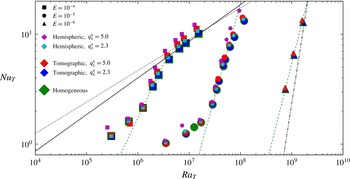
Figure 5 plots
 $Nu_{T}$
against
 $Ra_{T}$
for all of our simulations. For a given value of
 $E$
the slope of the
 $Nu$
–
 $Ra_{T}$
scaling is shallow at relatively low
 $Ra$
in the weakly nonlinear regime, steepens as the Rayleigh number increases, and shallows again at the highest values of
 $Ra_{T}$
, particularly for the runs with
 $E=10^{-4}$
(see also figures 6 and 7 for plots of several compensated
 $Nu$
scalings). Due to the computational expense we have performed a limited number of runs at
 $E=10^{-6}$
, concentrating on
 $Ra$
values where we expect to be in a regime of nonlinear rotating convection, which is our main region of interest. Gastine et al. (Reference Gastine, Wicht and Aubert2016) produced a regime diagram (their figure 20) showing that the rapidly rotating regime is expected for only a small span of
 $Ra_{T}$
for our values of
 $E$
, being bounded below by the weakly nonlinear regime (when
 $Ra\leqslant 6Ra_{C}$
) and above by a regime they term transitional, in which rotational effects no longer dominate even if the effectively non-rotating regime has not been reached. Our model has a different aspect ratio, radial gravity profile and thermal boundary conditions than Gastine et al. (Reference Gastine, Wicht and Aubert2016) so an exact correspondence between our results and their regime diagram is not to be expected; however, we observe similar regime transitions.
Compensated Nusselt number,
 $NuRa^{-2/7}$
, against proposed parameters controlling the transition out of the rotationally dominated regime. For clarity, and to focus on behaviour above the weakly nonlinear regime, only cases with
 $Ra_{F}>7Ra_{C}$
are shown. (a)
 $Ro_{C}=(RaE^{2}/Pr)^{1/2}$
, the convective Rossby number (Gilman Reference Gilman1977). (b)
 $RaE^{8/5}$
, based on the local Rossby number of the thermal boundary layer (Gastine et al.
Reference Gastine, Wicht and Aubert2016). (c)
 $RaE^{3/2}$
, based on thermal and viscous boundary layer crossing (King et al.
Reference King, Stellmach and Aurnou2012). Symbol shapes indicate the value of
 $E$
, symbol size and colour indicate the nature of the boundary conditions, as in figure 2.

Compensated versions of the Nusselt number as a function of Rayleigh number. In each case
 $Nu_{T}$
is divided by the value of
 $Nu_{T}$
for the homogeneous case at equivalent
 $Ra_{F}$
. For clarity, and to focus on behaviour above the weakly nonlinear regime, only cases with
 $Ra_{F}>7Ra_{C}$
are shown. Symbol colours, shapes and sizes as in figure 5. (a) Runs with
 $E=10^{-4}$
. (b) Runs with
 $E=10^{-5}$
. (c) Runs with
 $Tq_{L}^{\star }=5.0$
plotted as a function of supercriticality.

There is a clear decrease in the slope of the
 $Nu\propto Ra_{T}^{\unicode[STIX]{x1D6FE}}$
scaling for the highest
 $Ra_{T}$
cases with
 $E=10^{-4}$
; we do not, however, have sufficient results at high Rayleigh to adequately determine a best-fit scaling. As examples, in figure 5 we plot both
 $Nu\propto Ra_{T}^{1/3}$
and
 $Nu\propto Ra_{T}^{2/7}$
scalings for comparison with the highest Rayleigh number results with
 $E=10^{-4}$
. It is unlikely that a single scaling is appropriate over a wide range of Rayleigh number. Previous work in spherical geometry found that continuous changes in flow properties occur within the transitional regime (where our high-
 $Ra_{T}$
,
 $E=10^{-4}$
results lie), including a reduction in the exponent of the
 $Nu$
–
 $Ra_{T}$
scaling as supercriticality increases and the importance of rotational forces is progressively reduced (Gastine et al.
Reference Gastine, Wicht and Aurnou2015, Reference Gastine, Wicht and Aubert2016).
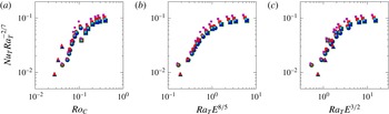
The transition from rotationally dominated to non-rotating convection corresponds to buoyancy becoming dominant over Coriolis forces; the most appropriate parameterisation of this transition remains an open question. In figure 6 we plot
 $NuRa_{T}^{-2/7}$
against three proposed transition parameters; to focus on the transition to the non-rotating regime at high Rayleigh number we plot only runs with
 $Ra_{F}>7Ra_{C}$
, which removes cases within the weakly nonlinear regime identified by Gastine et al. (Reference Gastine, Wicht and Aubert2016). The global-scale force balance can be expressed by the convective Rossby number,
 $Ro_{C}=(Ra_{T}E^{2}/Pr)^{1/2}$
, such that the transition to non-rotating convection might be expected when
 $Ro_{C}=O(1)$
(Gilman Reference Gilman1977; Zhong et al.
Reference Zhong, Stevens, Clercx, Verzicco, Lohse and Ahlers2009). We find that all of our runs have
 $Ro_{C}<1$
(figure 6
a) and do not support a
 $Ro_{C}=O(1)$
transition parameter, which agrees with previous numerical and laboratory studies (King et al.
Reference King, Stellmach, Noir, Hansen and Aurnou2009; Stellmach et al.
Reference Stellmach, Lischper, Julien, Vasil, Cheng, Ribeiro, King and Aurnou2014; Cheng et al.
Reference Cheng, Stellmach, Ribeiro, Grannan, King and Aurnou2015). Given the importance of the Ekman and thermal boundary layers in controlling heat transport through the system King et al. (Reference King, Stellmach and Aurnou2012) used the intersection of scaling laws for the thicknesses of these two boundary layers to suggest that the transition should occur for
 $Ra_{T}E^{3/2}=O(1)$
. If the transition is governed by the loss of geostrophic balance within the thermal boundary layer, scaling of the local Rossby number for the layer leads to a transition occurring at
 $Ra_{T}E^{8/5}=O(1)$
(Julien et al.
Reference Julien, Knobloch, Rubio and Vasil2012a
; Gastine et al.
Reference Gastine, Wicht and Aubert2016). This latter scaling does a somewhat better job of collapsing our results (compare figure 6
b,c). We would require significantly more high-
 $Ra$
runs to properly characterise both the slope of the
 $Nu$
–
 $Ra_{T}$
scaling and the transition parameter for the regime in which Coriolis effects no longer dominate buoyancy. Figures 5 and 6 suggests that few (if any) of our
 $E=10^{-4}$
runs fall within the nonlinear and rotationally dominated regime, but our runs at lower Ekman do sample this regime, a result consistent with the regime diagram of Gastine et al. (Reference Gastine, Wicht and Aubert2016).
We fit straight lines to each set of four consecutive runs (in terms of their
 $Ra$
) for the
 $q_{L}^{\star }=0$
simulations at
 $E=10^{-4}$
and
 $10^{-5}$
and take the line of best fit with maximum slope as the
 $Nu$
–
 $Ra_{T}$
scaling for the rotating regime. Although all of the runs that end up contributing to this fit may not be rotationally dominated, they are at least rotationally influenced. In both cases the line of steepest slope also corresponds to the four consecutive runs that are best fit by a straight line, although we note that these fits span a limited range of
 $Ra_{T}$
values. For
 $E=10^{-6}$
we fit a straight line to the three
 $q_{L}^{\star }=0$
simulations. As the Ekman number decreases, the exponent of the
 $Nu$
–
 $Ra_{T}$
scaling increases from 0.98 for
 $E=10^{-4}$
, to 1.69 for
 $E=10^{-5}$
, to 1.86 for
 $E=10^{-6}$
; such steepening of the
 $Nu$
–
 $Ra_{T}$
scaling with decreasing
 $E$
has previously been seen in both numerical and laboratory studies of rotating convection in a variety of geometries (e.g. King et al.
Reference King, Stellmach and Aurnou2012; Cheng et al.
Reference Cheng, Stellmach, Ribeiro, Grannan, King and Aurnou2015; Gastine et al.
Reference Gastine, Wicht and Aubert2016). Our scaling is steeper than the diffusivity-free scaling of
 $Nu\propto Ra_{T}^{3/2}E^{2}$
expected at low
 $E$
for convection with free-slip boundaries (Gillet & Jones Reference Gillet and Jones2006; Julien et al.
Reference Julien, Knobloch, Rubio and Vasil2012a
; Stellmach et al.
Reference Stellmach, Lischper, Julien, Vasil, Cheng, Ribeiro, King and Aurnou2014). We employ no-slip boundary conditions for which the effect of Ekman pumping has been shown to increase the efficiency of heat transport and hence the slope of the
 $Nu$
–
 $Ra_{T}$
scaling (Stellmach et al.
Reference Stellmach, Lischper, Julien, Vasil, Cheng, Ribeiro, King and Aurnou2014; Aurnou et al.
Reference Aurnou, Calkins, Cheng, Julien, King, Nieves, Soderlund and Stellmach2015; Julien et al.
Reference Julien, Aurnou, Calkins, Knobloch, Marti, Stellmach and Vasil2016). Although the scaling exponents for our low-
 $E$
runs lie above the diffusivity-free scaling, they are well below the scaling exponents of
 ${\sim}3$
found in studies with no-slip boundaries in cylindrical and Cartesian geometries at similar
 $E$
(King et al.
Reference King, Stellmach and Aurnou2012; Cheng et al.
Reference Cheng, Stellmach, Ribeiro, Grannan, King and Aurnou2015).
3.3
 $Nu$
enhancement by heterogeneous boundaries

Our particular interest is whether different boundary heterogeneities alter the amplitude of
 $Nu$
for a given value of
 $Ra$
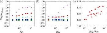
or even the slope of the associated scaling law; to more clearly show such differences figure 7 presents compensated
 $Nu$
values. In this figure, the
 $Nu$
for each run is divided by the value obtained from the
 $q_{L}^{\star }=0$
case at the same
 $Ra_{F}$
. There is little difference between the
 $Tq_{L}^{\star }=2.3$
cases and the equivalent
 $q_{L}^{\star }=0$
cases. However, in the other cases the heterogeneity in outer boundary heat flux tends to enhance the efficiency of heat transport; the enhancement tends to become greater as
 $Ra$
becomes more supercritical, the wavelength of the imposed boundary heterogeneity increases, or the amplitude of
 $q_{L}^{\star }$
increases. Investigations of relatively low-
 $Ra$
convection in high-
 $Pr$
fluids (Zhang & Gubbins Reference Zhang and Gubbins1993; Davies et al.
Reference Davies, Gubbins and Jimack2009) have found that the effect of outer boundary heterogeneity on the underlying fluid is greater when larger-wavelength lateral variations are applied, consistent with our results at
 $Pr=1$
and more highly supercritical
 $Ra$
.
We find that addition of outer boundary heterogeneity tends to increase
 $Nu$
relative to equivalent
 $q_{L}^{\star }=0$
cases, whereas Dietrich et al. (Reference Dietrich, Hori and Wicht2016) found a nearly linear reduction in
 $Nu$
with increasing
 $Hq_{L}^{\star }$
for simulations with
 $Ra/Ra_{C}=25$
,
 $E=10^{-4}$
and a range of
 $0\leqslant Hq_{L}^{\star }\leqslant 2.0$
(see figures 11 and 13 of their paper and note that their definition of
 $q^{\star }$
is equal to one half our
 $Hq_{L}^{\star }$
). This difference arises from the fact that we use
 $\overline{\langle \unicode[STIX]{x0394}T\rangle }$
in determining
 $Nu_{T}$
, whereas Dietrich et al. (Reference Dietrich, Hori and Wicht2016) estimate
 $\unicode[STIX]{x0394}T=T_{max}-T_{min}$
, where
 $T_{max}$
and
 $T_{min}$
are the maximum and minimum values of
 $T$
in the domain (Dietrich, personal communication). When there are large lateral variations in boundary heat flux, and hence fluid temperature, the point-wise maximum approach can significantly overestimate the average temperature drop across the system and thus underestimate
 $Nu_{T}$
. We have found that calculating
 $\overline{\langle \unicode[STIX]{x0394}T\rangle }$
for their simulations yields an increase in
 $Nu$
for boundary-forced cases compared to the corresponding homogeneous case.
Differences in the Nusselt number between our
 $Hq_{L}^{\star }=5.0$
and
 $q_{L}^{\star }=0$
cases at equivalent
 $Ra_{F}$
can be as much as 20–25 % and appear to saturate as the simulations reach the regime where rotation no longer dominates the force balance; this saturation effect is most evident for our
 $E=10^{-4}$
cases (figure 7
a) as the regime without rotational dominance is more easily reached for larger Ekman number. Since the difference in
 $Nu$
between the
 $Hq_{L}^{\star }=5.0$
and
 $q_{L}^{\star }=0$
cases grows with
 $Ra$
in the rotationally dominated regime, they are characterised by different exponents for the
 $Nu$
–
 $Ra_{T}$
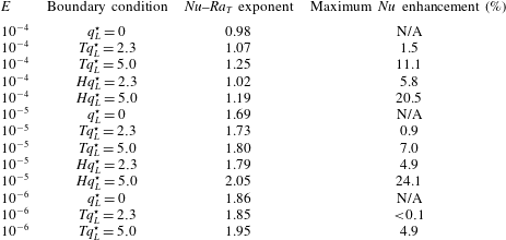
scaling; for example, we find an exponent of 2.05 for
 $E=10^{-5}$
and
 $Hq_{L}^{\star }=5.0$
, significantly above the 1.69 exponent for
 $q_{L}^{\star }=0$
. Although each scaling determination uses only four simulations from a relatively limited range of
 $Ra_{T}$
the enhanced efficiency of heat transport in the
 $Hq_{L}^{\star }=5.0$
cases is clear and much greater than the
 $Hq_{L}^{\star }=2.3$
cases, which reach at most
 ${\sim}5\,\%$
enhancement. For the
 $Tq_{L}^{\star }=5.0$
cases enhancements of about 5 %–10 % are obtained for the three Ekman numbers we consider, with a decrease in the enhancement of
 $Nu$
as
 $E$
is lowered (figure 7
c). For our lowest
 $E$
cases we have not been able to reach the regime where rotation no longer dominates the force balance; we expect that the enhancement of the Nusselt number would continue to increase with supercriticality within the rapidly rotating regime, before saturating at sufficiently large
 $Ra_{F}/Ra_{C}$
.
To better understand the
 $Nu$
enhancement by boundary heterogeneity we consider, as an example, the simulations with
 $E=10^{-5}$
and the highest applied Rayleigh number (
 $Ra_{F}=1.3\times 10^{9}$
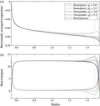
). In figure 8 we plot radial profiles of temperature,
 $\langle \overline{T^{\star }}\rangle$
, advective heat transport,
 $4\unicode[STIX]{x03C0}{r^{\star }}^{2}\langle \overline{u_{r}^{\star }T^{\star }}\rangle$
, and diffusive heat transport,
 $4\unicode[STIX]{x03C0}{r^{\star }}^{2}\langle \overline{-\unicode[STIX]{x2202}T^{\star }/\unicode[STIX]{x2202}r^{\star }}\rangle$
. All five cases have thermal boundary layers at the top and bottom of the shell, with the inner boundary layer being more pronounced, and a small but non-zero temperature gradient in the shell interior. For the purposes of plotting
 $\langle \overline{T^{\star }}\rangle$
has been set to zero at the inner boundary; differences in
 $\langle \overline{\unicode[STIX]{x0394}T^{\star }}\rangle$
are thus reflected by the average temperatures plotted at
 $r_{o}^{\star }$
. The shape of the temperature profiles for the two
 $q_{L}^{\star }=5.0$
runs is noticeably different near the top of the shell, with the development of a local maximum in
 $\langle \overline{T^{\star }}\rangle$
and hence a region where the radial temperature gradient is positive. There is a corresponding change in the diffusive contribution to the heat transport such that for both of these
 $q_{L}^{\star }=5.0$
runs there is a depth range near the outer boundary where the net diffusive transport of heat is negative, that is, radially inwards. Since
 $4\unicode[STIX]{x03C0}r^{2}\langle \overline{\boldsymbol{q}}\boldsymbol{\cdot }\hat{\boldsymbol{r}}\rangle$
is conserved, any change in the diffusive contribution is offset by an equal but opposite change in the advective contribution. For the heterogeneous runs shown in figure 8 the modification in heat transport relative to the homogeneous case is constrained to the outer regions of the shell, with larger amplitude and longer-wavelength heterogeneity resulting in changes that extend more deeply.
(a) Radial profiles of
 $\langle \overline{T^{\star }}\rangle$
for runs with
 $E=10^{-5}$
and
 $Ra_{F}=1.3\times 10^{9}$
; boundary conditions are indicated by colour and line style. In all cases temperature is set to zero on the inner boundary for the purpose of plotting. (b) Profiles of temporally averaged radial heat flow for these runs, solid lines indicate the advective contribution, dashed lines indicate the diffusive contribution; the boundary conditions are indicated by colour as in (a). The vertical dashed line indicates the radius for which maps and spectra are plotted in figure 9.

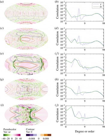
Flow and temperature correlations at a radius of
 $r^{\star }=1.48$
for all of the runs with
 $E=10^{-5}$
and
 $Ra_{F}=1.3\times 10^{9}$
; from (a–j) the boundary conditions are:
 $q_{L}^{\star }=0$
,
 $Tq_{L}^{\star }=2.3$
,
 $Tq_{L}^{\star }=5.0$
,
 $Hq_{L}^{\star }=2.3$
,
 $Hq_{L}^{\star }=5.0$
. (a,c,e,g,i) Maps of radial velocity (green–magenta) overlain with contours of temperature anomaly (purple–orange); the projection is centred on the negative
 $x$
-axis, thus
 $q_{max}$
is centred for the
 $Hq_{L}^{\star }$
cases and one of the
 $q_{min}$
is approximately centred for the
 $Tq_{L}^{\star }$
cases. (b,d,f,h,j) Spectra of
 $\overline{u_{r}^{\star }T^{\star }}$
;
 $\ell$
-spectra (i.e. integration over all
 $m$
and
 $r$
for fixed
 $\ell$
, dashed blue line),
 $m$
-spectra (i.e. integration over all
 $\ell$
and
 $r$
for fixed
 $m$
, solid green line). For the purpose of plotting, spectra are truncated at
 $\ell =m=99$
.

In figure 9 we plot maps of
 $\overline{u_{r}^{\star }}$
overlain by contours of temperature anomaly,
 $\overline{T^{\star }}-\langle \overline{T^{\star }}\rangle$
, as well as the spectra of
 $(\ell (\ell +1)/(2\ell +1))\overline{p_{\ell }^{m}\unicode[STIX]{x1D717}_{\ell }^{m}}$
. In all cases these quantities have been determined for a radius of
 $r^{\star }=1.48$
(the vertical dashed line in figure 8), which lies near the peak in advective heat transport for the
 $q_{L}^{\star }=5.0$
cases. For the
 $q_{L}^{\star }=0$
case the largest single contribution to the advective heat transport comes from the
 $Y_{4}^{0}$
harmonic; the small-scale convection makes a secondary contribution, with a broad peak in the correlation between
 $u_{r}^{\star }$
and
 $T^{\star }$
centred at spherical harmonics of approximately degree and order 40. For this
 $q_{L}^{\star }=0$
case the polar regions are relatively hot in the time average and temperature anomalies at low to mid-latitudes are weak. For the runs with heterogeneous outer boundaries there is an increased correlation between
 $u_{r}^{\star }$
and
 $T^{\star }$
at long wavelengths, with particular enhancement in advective heat transport at spherical harmonics that match the imposed boundary conditions. The contributions identified in the spectra of the homogeneous case are still present, but become relatively less important to the total advective transport as
 $q_{L}^{\star }$
is increased.
For these runs anomalously hot material accumulates near the top of the fluid shell under
 $q_{min}$
. The formation of small-scale convection rolls is suppressed in these hot regions, with a broad region of relatively weak outward flow favoured instead. The heterogeneous runs also have regions where downwelling is promoted; the time average of the
 $q_{L}^{\star }=5.0$
runs have regions of particularly intense downwelling near the western edges of the anomalously hot regions. Individual snapshots of the flow show the suppression of small-scale convection under
 $q_{min}$
; however, the focusing of downwelling is not obvious, emerging only in the time average. The promotion of downwelling at the western boundary of hot regions in these simulations is similar to the jet development observed by Sumita & Olson (Reference Sumita and Olson1999, Reference Sumita and Olson2002) at the front between hot and cold regions in their physical experiment. However, in our numerical simulations the formation of a single spiralling front that spans the shell is prevented by the presence of strong zonal flows of alternating sign in the shell interior. Regardless, the formation of broad regions of weak upwelling and focused regions of enhanced downwelling tends to increase advective heat transport near the top of the shell in these heterogeneous cases and hence raise the Nusselt number relative to the homogeneous case. For the
 $Tq_{L}^{\star }=2.3$
case there is increased advective transport relative to the homogeneous case at some spherical harmonics, most substantially at
 $Y_{2}^{2}$
; however, these increases do not offset a reduction in the
 $Y_{4}^{0}$
contribution by
 ${\sim}15\,\%$
. For the
 $Tq_{L}^{\star }=5.0$
case the reduction in the
 $Y_{4}^{0}$
contribution relative to
 $q_{L}^{\star }=0$
is much smaller (
 ${\sim}1\,\%$
) and is more than compensated by increased advective transport at other harmonics. For the
 $Hq_{L}^{\star }=2.3$
case the
 $Y_{4}^{0}$
contribution at this radius is increased relative to the homogeneous case by
 ${\sim}10\,\%$
; the relative increase in advective heat transport at
 $Y_{1}^{1}$
is much larger, but the absolute difference is similar for both harmonics. For the
 $Hq_{L}^{\star }=5.0$
case the Nusselt number enhancement is dominated by the increased correlation between radial velocity and temperature at
 $Y_{1}^{1}$
. The results in figure 9 are for one particular radius and a single set of simulations, but are representative of the changes seen near the top of the fluid layer when heterogeneous boundary conditions are imposed.
All simulations for which the heterogeneous outer boundary condition increases the Nusselt number must do so by increasing the radial advective transport of heat over some radial extent, which is generally restricted towards the outer regions of the shell in our simulations. There is a corresponding reduction in the diffusive contribution to radial heat transport and thus
 $\langle \overline{\unicode[STIX]{x2202}T/\unicode[STIX]{x2202}r}\rangle$
becomes less negative in the affected region, relative to the equivalent homogeneous case. In some of our simulations (for example, the
 $q_{L}^{\star }=5.0$
cases in figure 8) the time-averaged temperature gradient even becomes positive in a region near the outer boundary, an apparent stable stratification. In principle, our use of the Boussinesq approximation could be invalidated in such cases. The Boussinesq approximation requires that density variation across the system in the background state is sufficiently small (Spiegel & Veronis Reference Spiegel and Veronis1960). Although commonly used in models of planetary cores, this thin layer approximation is only marginally satisfied for Earth’s core (see e.g. Jones Reference Jones and Schubert2015), which remains true for our investigation. The Boussinesq approximation would also be invalid if the system dynamics produces sufficiently large fluctuations in density (Spiegel & Veronis Reference Spiegel and Veronis1960). Although the time-averaged temperature anomalies in our most extreme heterogeneous cases are large compared to those found in homogeneous convection, the fluctuations at any point in time remain smaller than the static variations of the background state and the Boussinesq approximation still holds.
The large lateral variations in the time-averaged temperature near the top of the shell that arise in these cases are associated with strong variations in local dynamics, with regions of both inhibited and enhanced small-scale convection (figure 9). This situation is in some sense the complement of the physical experiments of Alboussière, Deguen & Melzani (Reference Alboussière, Deguen and Melzani2010) investigating stratification at the bottom of the core due to partial melting of the inner core; they injected fluids that were both compositionally dense and buoyant at the bottom of a tank and found that the upwellings of buoyant fluid did not prevent the formation of a dense, stably stratified layer. We have strong lateral variations in thermal buoyancy generated at the top of the shell; however, the strong localised convection does not preclude the formation of an average stratification, as in the physical experiment. Stratification at the top of Earth’s core has been hypothesised based on both seismic and geomagnetic observations, with both thermal and compositional stratification mechanisms proposed (see e.g. Helffrich & Kaneshima Reference Helffrich and Kaneshima2013). Heterogeneous outer boundary conditions that increase
 $Nu$
by reorganising flow near the top of the core will necessarily make the average radial temperature gradient more positive in the affected region and can potentially create a thermal stratification signature in the average temperature profile.
4 Conclusions
In planetary settings it is expected that long-wavelength variations in the heat flux at the top of metallic cores beneath convecting silicate mantles will be common, although the pattern and amplitude of these variations are uncertain and will vary both between bodies and through time. We have performed 106 numerical simulations, with three Ekman numbers and five different thermal boundary conditions to investigate how heat transport by thermal convection in rotating spherical shells is impacted by the inclusion of heterogeneous heat flux at the outer boundary. The large amplitude and long-wavelength boundary heterogeneity we considered tends to increase the Nusselt number of the system relative to equivalent homogeneous cases (table 2).
The size of the Nusselt number enhancement tends to increase as the amplitude and wavelength of the boundary heterogeneity increases. The enhancement also tends to increase with the supercriticality of the system, although it may saturate as the system enters the regime in which rotation no longer dominates the force balance. This Rayleigh-dependent enhancement can significantly steepen the
 $Nu-Ra_{T}$
scaling within the rotationally dominated regime, particularly for the
 $q_{L}^{\star }=5.0$
cases. The Nusselt number enhancement arises from an increased correlation between radial flow and temperature, particularly near the top of the shell, due to the development of regions of broad weak upwelling with relatively narrow regions at their western edge where downwelling is strongly promoted. The fixed-flux boundary conditions require that any increase in the advective contribution to the time-averaged radial heat transport is accompanied by a decrease in the diffusive contribution and hence a modification of the time-averaged temperature profile. In our simulations these effects generally occur near the top of the shell and in some cases can produce an apparent thermal stratification in the time-averaged temperature profile, despite the presence of regions of strong convection at all radii.
Heat transport enhancement results organised by Ekman number and applied boundary condition: exponent of the
 $Nu\propto Ra_{T}^{\unicode[STIX]{x1D6FE}}$
scaling in the rotationally dominated regime; and the largest seen enhancement of
 $Nu$
relative to the equivalent homogeneous
 $Ra_{F}$
case.

Acknowledgements
C.J.D. is supported by Natural Environment Research Council independent research fellowship NE/L011328/1 and a Green scholarship at IGPP. W. Dietrich and J. Aurnou are thanked for fruitful discussion as are three anonymous reviewers for their suggestions that improved this work. This work used the ARCHER UK National Supercomputing Service (http://www.archer.ac.uk) and ARC2, part of the High Performance Computing facilities at the University of Leeds, UK. Figures were produced using VisIt (Childs et al. Reference Childs, Brugger, Whitlock, Meredith, Ahern, Pugmire, Biagas, Miller, Harrison, Weber, Wes Bethel, Childs and Hansen2012) and Matplotlib (Hunter Reference Hunter2007).
Appendix A. The non-dimensionalisation of
$\unicode[STIX]{x0394}T_{C}$

The temperature drop across the spherical shell with fixed-flux boundary conditions in our pure conduction case is
 $\unicode[STIX]{x0394}T_{C}=\unicode[STIX]{x1D6FD}h/r_{i}r_{o}$
(2.25). After non-dimensionalisation of length by
 $h=r_{o}-r_{i}$
and temperature by
 $\unicode[STIX]{x1D6FD}/h$
we have
 $$\begin{eqnarray}\unicode[STIX]{x0394}T_{C}^{\star }=\frac{1}{r_{i}^{\star }r_{o}^{\star }}.\end{eqnarray}$$
Therefore, when expressed in terms of the non-dimensional temperature we have
 $$\begin{eqnarray}Nu_{T^{\star }}=\frac{r_{i}^{\star }r_{o}^{\star }}{\unicode[STIX]{x0394}\langle \overline{T^{\star }}\rangle }.\end{eqnarray}$$
We set our model to match Earth, so
 $r_{i}=1.22\times 10^{6}$
m,
 $r_{o}=3.48\times 10^{6}$
m and thus
 $Nu_{T^{\star }}\approx 1.2/\unicode[STIX]{x0394}\langle \overline{T^{\star }}\rangle$
. We highlight this result in contrast to the plane layer geometry for which
 $Nu_{T^{\star }}=1/\unicode[STIX]{x0394}\langle \overline{T^{\star }}\rangle$
(e.g. Otero et al.
Reference Otero, Wittenberg, Worthing and Doering2002).
Since our temperature scaling depends on shell geometry, it is possible to construct a spherical shell for which
 $Nu_{T^{\star }}=1$
as in the plane layer case. The combination of temperature and length non-dimensionalisation would then imply
 $$\begin{eqnarray}\displaystyle & \displaystyle 1=\frac{1}{r_{i}^{\star }r_{o}^{\star }}, & \displaystyle\end{eqnarray}$$
 $$\begin{eqnarray}\displaystyle & 1=r_{o}^{\star }-r_{i}^{\star }. & \displaystyle\end{eqnarray}$$
The solution is
 $$\begin{eqnarray}\displaystyle & \displaystyle r_{i}^{\star }=\frac{\sqrt{5}}{2}-\frac{1}{2}=\frac{1}{\unicode[STIX]{x1D711}}, & \displaystyle\end{eqnarray}$$
 $$\begin{eqnarray}\displaystyle & \displaystyle r_{o}^{\star }=\frac{\sqrt{5}}{2}+\frac{1}{2}=\unicode[STIX]{x1D711}, & \displaystyle\end{eqnarray}$$
giving a radius ratio
 $r_{i}/r_{o}=1/\unicode[STIX]{x1D711}^{2}\approx 0.382$
, not far from the value of
 ${\sim}0.351$
for Earth.
Summary of all runs for
 $E=10^{-4}$
.

Summary of all runs with
 $E=10^{-5}$
.

Summary of all runs with
 $E=10^{-6}$
.

Appendix B. Tables of results
Summary tables of the model resolution, control parameters and selected output parameters for all simulations. In all cases
 $Pr=1$
and the radius ratio
 $r_{i}/r_{o}=0.351$
.
 $N_{r}$
is the number of radial points within the fluid shell.
 $N_{\unicode[STIX]{x1D6FF}i}$
and
 $N_{\unicode[STIX]{x1D6FF}o}$
are the number of radial points within the mechanical boundary layer at the inner and outer boundary, respectively.
 $\ell _{max}=m_{max}$
is the maximum degree and order of spherical harmonic expansion. Definitions of the Ekman number and modified Rayleigh number are given in (2.10). The amplitude of the heterogeneity in outer boundary heat flux is defined in (1.1);
 $q_{L}^{\star }=0$
are homogeneous cases,
 $Tq_{L}^{\star }$
are cases with a pattern of heat flux derived from mantle tomography,
 $Hq_{L}^{\star }$
are cases with a hemispheric (
 $Y_{1}^{1}$
) pattern.
 $Nu_{T}$
is given by (2.30). The Reynolds number is determined by (2.16) and hence the kinetic energy integral (2.17).
 $Re_{pol}$
is found by retaining only the poloidal component of velocity (recall (2.4)) in the kinetic energy integral.
 $Re_{zon}$
is found by retaining only the
 $m=0$
components from the spherical harmonic expansion of the toroidal component of velocity in the kinetic energy integral.
 $P$
is the time average of the buoyancy production throughout the shell,
 $\unicode[STIX]{x1D716}_{U}$
is the time average of the viscous dissipation throughout the shell.