


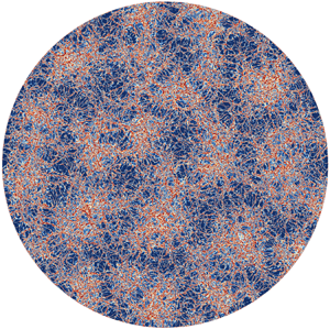





1. Introduction
Rayleigh–Bénard convection (RBC) is the most widely studied model of thermal convection (Ahlers, Grossmann & Lohse Reference Ahlers, Grossmann and Lohse2009; Lohse & Xia Reference Lohse and Xia2010; Chilla & Schumacher Reference Chilla and Schumacher2012; Xia Reference Xia2013; Shishkina Reference Shishkina2021; Lohse & Shishkina Reference Lohse and Shishkina2023; Xia et al. Reference Xia, Huang, Xie and Zhang2023). This model's dimensionless control parameters are the Rayleigh number  ${{Ra}}$ and the Prandtl number
 ${Pr}$, which respectively characterize the dimensionless temperature difference and fluid properties, and the aspect ratio
 $\varGamma$, which is defined as the system's width over height. The unifying theory of thermal convection has significantly advanced the theoretical understanding of the flow's global transfer properties (Grossmann & Lohse Reference Grossmann and Lohse2000, Reference Grossmann and Lohse2001, Reference Grossmann and Lohse2002, Reference Grossmann and Lohse2004; Ahlers et al. Reference Ahlers, Grossmann and Lohse2009; Stevens et al. Reference Stevens, van der Poel, Grossmann and Lohse2013). This Grossmann–Lohse (GL) theory accurately predicts the relationship between the Nusselt number
 ${{Nu}}$ (the non-dimensionalized heat transport) and the Reynolds number
 ${Re}$ (the non-dimensionalized flow strength) as a function of
 ${{Ra}}$ and
 ${Pr}$.
Observations at moderate  ${{Ra}}$ values have demonstrated that appropriate lateral confinement can significantly enhance heat transport, due to the enhancement of vertically coherent flow structures (Huang et al. Reference Huang, Kaczorowski, Ni and Xia2013; Chong et al. Reference Chong, Huang, Kaczorowski and Xia2015, Reference Chong, Yang, Huang, Zhong, Stevens, Verzicco, Lohse and Xia2017; Zhang & Xia Reference Zhang and Xia2023; Ren et al. Reference Ren, Tao, Xia and Xie2024). Moreover, Hartmann et al. (Reference Hartmann, Chong, Stevens, Verzicco and Lohse2021) showed that the extent of heat transfer enhancement due to confinement depends strongly on the system's geometry, with a greater enhancement observed in cylindrical cells compared to rectangular or square ones.
Both the onset of convection and the transition to the ultimate regime occur at significantly higher  ${{Ra}}$ in very small aspect ratio cells. Theoretical and numerical studies have quantified the increase in the critical Rayleigh number
 ${{Ra}}_c$ for the onset of convection (see e.g. Charlson & Sani Reference Charlson and Sani1970) and the typical Rayleigh numbers
 ${{Ra}}^*$ for the transition to the ultimate regime, namely as
 ${{Ra}}_c \propto \varGamma ^{-4}$ for the onset of convection (Shishkina Reference Shishkina2021; Ahlers et al. Reference Ahlers2022; Zhang & Xia Reference Zhang and Xia2023; Ren et al. Reference Ren, Tao, Xia and Xie2024) and as
 ${{Ra}}^* \propto \varGamma ^{-3}$ for the onset of the ultimate regime (Roche et al. Reference Roche, Gauthier, Kaiser and Salort2010; Roche Reference Roche2020; Ahlers et al. Reference Ahlers2022). The existence of an ultimate regime with enhanced heat transport properties and turbulent boundary layers (BLs) had initially been predicted by Kraichnan (Reference Kraichnan1962) and later by Spiegel (Reference Spiegel1972) and by Grossmann & Lohse (Reference Grossmann and Lohse2000, Reference Grossmann and Lohse2001, Reference Grossmann and Lohse2011). The transition to the ultimate regime has meanwhile been observed in various experiments (Chavanne et al. Reference Chavanne, Chilla, Castaing, Hebral, Chabaud and Chaussy1997; Roche et al. Reference Roche, Gauthier, Kaiser and Salort2010; He et al. Reference He, Funfschilling, Nobach, Bodenschatz and Ahlers2012) and has been interpreted to be of non-normal nonlinear type (Roche Reference Roche2020; Lohse & Shishkina Reference Lohse and Shishkina2023). The simulations presented in this present work do not reach the ultimate regime, which therefore is not discussed further in the main part of this paper, and is readdressed only in the final outlook part of the conclusions.
In nature, convection frequently occurs in very large to infinite domains, facilitating the formation of large-scale turbulent superstructures. For RBC just above the onset, numerous experiments (Fitzjarrald Reference Fitzjarrald1976; Bodenschatz, Pesch & Ahlers Reference Bodenschatz, Pesch and Ahlers2000; Sun et al. Reference Sun, Ren, Song and Xia2005; du Puits, Resagk & Thess Reference du Puits, Resagk and Thess2007; Xia, Sun & Cheung Reference Xia, Sun and Cheung2008; Zhou et al. Reference Zhou, Liu, Li and Zhong2012; Hogg & Ahlers Reference Hogg and Ahlers2013; du Puits, Resagk & Thess Reference du Puits, Resagk and Thess2013) and simulations conducted in large periodic domains (Hartlep, Tilgner & Busse Reference Hartlep, Tilgner and Busse2003; Parodi et al. Reference Parodi, von Hardenberg, Passoni, Provenzale and Spiegel2004; Hartlep, Tilgner & Busse Reference Hartlep, Tilgner and Busse2005; von Hardenberg et al. Reference von Hardenberg, Parodi, Passoni, Provenzale and Spiegel2008) as well as in very large aspect ratio cylindrical domains (Shishkina & Wagner Reference Shishkina and Wagner2005, Reference Shishkina and Wagner2006; Bailon-Cuba, Emran & Schumacher Reference Bailon-Cuba, Emran and Schumacher2010; Emran & Schumacher Reference Emran and Schumacher2015; Sakievich, Peet & Adrian Reference Sakievich, Peet and Adrian2016) have unveiled remarkable flow patterns. Correlations between single-point measurements (du Puits et al. Reference du Puits, Resagk and Thess2007, Reference du Puits, Resagk and Thess2013) and particle image velocimetry measurements (Xia et al. Reference Xia, Sun and Cheung2008) have indicated a transition from a single-roll to a multi-roll structure as  $\varGamma$ exceeds approximately 4.
Recent simulations by Stevens et al. (Reference Stevens, Blass, Zhu, Verzicco and Lohse2018) have revealed that turbulent superstructures persist up to  ${{Ra}}=10^9$, with the size of these superstructures increasing with
 ${{Ra}}$, at least up to
 ${{Ra}}=10^9$. Visualizations by Pandey, Scheel & Schumacher (Reference Pandey, Scheel and Schumacher2018) and Stevens et al. (Reference Stevens, Blass, Zhu, Verzicco and Lohse2018) suggest that large-scale structures are more pronounced in the temperature field than in the velocity field. However, a scale-by-scale analysis using the linear coherence spectrum to examine the correlation between the two fields reveals a near-perfect correlation at the superstructure scale (Krug, Lohse & Stevens Reference Krug, Lohse and Stevens2020). Furthermore, it has been demonstrated that approximately
 $30\,\%$ of the heat transfer can be attributed to these large-scale flow structures. As the organization of the large-scale flow varies with
 $\varGamma$, the heat transport in the large aspect ratio limit (
 $\varGamma \gtrsim 4$) is found to be approximately
 $10\,\%$ lower for
 ${{Ra}}=2 \times 10^7$ and approximately
 $4\,\%$ lower for
 ${{Ra}}=10^9$ compared to
 $\varGamma =1$ (Stevens et al. Reference Stevens, Blass, Zhu, Verzicco and Lohse2018).
Despite these efforts, the flow characteristics in large aspect ratio RBC remain insufficiently documented and understood. Notably, direct one-to-one comparisons between laterally periodic and confined domain simulations have not been performed. Previous simulations for large  $\varGamma$ in cylindrical cells (Bailon-Cuba et al. Reference Bailon-Cuba, Emran and Schumacher2010) failed (for the reason, refer to the Appendix) to identify a large-
 $\varGamma$ limit, which in contrast was observed in periodic domains (Stevens et al. Reference Stevens, Blass, Zhu, Verzicco and Lohse2018). To bridge this gap in the literature, in this paper we perform direct numerical simulations (DNS) in unprecedentedly large cylindrical domains,
 $0.075 \leqslant \varGamma \leqslant 32$, achieving up to
 ${{Ra}}=10^8$. This allows for direct comparisons between cylindrical domains and laterally periodic domains in the limit of very large aspect ratios, showing that the main flow characteristics within these domains become identical as the aspect ratio increases.
The remainder of the paper is organized as follows. Section 2 provides details of the simulation dataset. Section 3 discusses the evolution of  ${{Nu}}$ and integral
 ${Re}$ as a function of
 $\varGamma$. Subsequently, in § 4, we analyse the effects of the system geometry and
 $\varGamma$ on the flow structures and velocity and temperature variance distributions in the domain. The paper ends with a summary, conclusions, and an outlook (§ 5).
2. Simulations
We perform DNS of RBC in large cylindrical domains with aspect ratios  $0.075\leqslant \varGamma \leq 32$, solving the incompressible Navier–Stokes equations and the heat transfer equation in Oberbeck–Boussinesq approximation (Ahlers et al. Reference Ahlers, Grossmann and Lohse2009). The simulations employ a second-order, energy-conserving finite difference method. This method was initially developed by Verzicco & Orlandi (Reference Verzicco and Orlandi1996) and Verzicco & Camussi (Reference Verzicco and Camussi1997), and has been validated extensively against experiments (Stevens, Verzicco & Lohse Reference Stevens, Verzicco and Lohse2010b; Stevens, Lohse & Verzicco Reference Stevens, Lohse and Verzicco2011; Stevens et al. Reference Stevens, van der Poel, Grossmann and Lohse2013). Its latest optimized version used here is validated against spectral element methods and fourth-order finite volume schemes (Kooij et al. Reference Kooij, Botchev, Frederix, Geurts, Horn, Lohse, van der Poel, Shishkina, Stevens and Verzicco2018).
The control parameters are defined as  ${{Ra}} = \alpha g\varDelta L^3 / (\nu \kappa )$ and
 ${Pr} = \nu / \kappa$, where
 $\alpha$ represents the thermal expansion coefficient,
 $g$ is the gravitational acceleration,
 $\varDelta$ denotes the temperature difference between the top and bottom plates,
 $L$ is the height of the fluid domain,
 $\nu$ is the kinematic viscosity, and
 $\kappa$ is the thermal diffusivity of the fluid. In total, 20 simulations were conducted for
 ${{Ra}}=2\times 10^7$ and
 $10^8$, while
 ${Pr}$ is fixed at 1. The bottom and top plates were assigned no-slip, constant-temperature boundary conditions, while the sidewall was treated as no-slip and adiabatic.
All simulations were executed carefully to ensure consistency, following the resolution criteria established in previous works (Shishkina et al. Reference Shishkina, Stevens, Grossmann and Lohse2010; Stevens et al. Reference Stevens, Verzicco and Lohse2010b). In this context, we also refer to the supplementary material of Ahlers et al. (Reference Ahlers2022), which in its § III explicitly states the requirements on the quality of DNS of turbulent thermal convection, with respect to both spatial resolution and time averaging. To give an example on the resolution, the  ${{Ra}} = 10^8$ and
 $\varGamma = 32$ simulation was conducted on an
 $18\,432 \times 3072 \times 192$ grid. The statistical convergence of integral flow quantities, such as
 ${{Nu}}$ and
 ${Re}$, was within a fraction of 1 %. Achieving such excellent convergence is highly challenging and relies on meticulous simulation design. Due to the slow dynamics of the thermal superstructures, the convergence of higher-order statistics is inevitably less good than for the integral flow characteristics. The simulations were performed for very long durations, specifically for
 $\varGamma >1$,
 ${\approx }750$ dimensionless time units (measured as all times in terms of
 $L/U_{ff}$, where
 $U_{ff} = \sqrt {\alpha g \varDelta L}$ is the free-fall velocity) for
 ${{Ra}} = 2\times 10^7$, and
 ${\approx }500$ time units at
 ${{Ra}} = 10^8$. For
 $\varGamma \lesssim 1$, 1000 to 10 000 dimensionless time units were considered. The first 100 time units were disregarded as transients. These simulation times exceed the typical duration considered in RBC simulations. Despite the simulations being conducted for extended periods, the recorded flow dynamics in the form of movies indicates that the time required for thermal superstructures to alter their position within the vast domains exceeds the duration of our simulations.
3. Integral heat transport and flow strength
For Rayleigh–Bénard flow in the cylindrical cell, and very small aspect ratio  $\varGamma$ (very slender cells), the Nusselt number is 1, i.e. pure diffusive transport, due to the stabilization by the sidewalls. The critical aspect ratio
 $\varGamma _c$ beyond convection sets in depends on
 ${{Ra}}$ as
 $\varGamma _c \propto {{Ra}}^{-1/4}$ (Shishkina Reference Shishkina2021; Ahlers et al. Reference Ahlers2022; Zhang & Xia Reference Zhang and Xia2023; Ren et al. Reference Ren, Tao, Xia and Xie2024). When further increasing
 $\varGamma$, one obtains a maximum in
 ${{Nu}}/{{Ra}}^{1/3}$, as can be seen from figure 1(a). The maximal heat transport is due to the stabilization of the large-scale convection (LSC) due to intermediate confinement. This effect has been observed previously in rectangular cells (Huang et al. Reference Huang, Kaczorowski, Ni and Xia2013; Chong et al. Reference Chong, Huang, Kaczorowski and Xia2015, Reference Chong, Yang, Huang, Zhong, Stevens, Verzicco, Lohse and Xia2017), and more recently in square and cylindrical domains (Hartmann et al. Reference Hartmann, Chong, Stevens, Verzicco and Lohse2021, Reference Hartmann, Verzicco, Kranenbarg, Lohse and Stevens2022; Zhang & Xia Reference Zhang and Xia2023; Ren et al. Reference Ren, Tao, Xia and Xie2024). Beyond the maximum, with again further increasing aspect ratio,
 ${{Nu}}/{{Ra}}^{1/3}$ decreases again, before reaching a plateau value beyond
 $\varGamma \gtrsim 4$. We performed well-resolved numerical simulations with aspect ratios as large as
 $\varGamma = 32$. We note that beyond
 $\varGamma \gtrsim 4$ (or even not beyond the position of the maximum at
 $\varGamma \approx 0.3$ or even less for higher
 ${{Ra}}$), there is no increase of the heat transport with increasing
 $\varGamma$, as was erroneously stated in Bailon-Cuba et al. (Reference Bailon-Cuba, Emran and Schumacher2010). In that publication, the increase of the heat transfer with increasing
 $\varGamma$ is due to increasingly insufficient grid resolution; see the Appendix.
(a) Dimensionless heat transport  ${{Nu}}$ and (b) total, (c) vertical and (d) horizontal Reynolds numbers
 ${Re}_{tot}$,
 ${Re}_z$ and
 ${Re}_{\mathscr {H}}$, respectively, as functions of
 $\varGamma$ in a periodic and cylindrical domain for
 ${{Ra}}=2\times 10^7$ and
 $10^8$ (periodic data from Stevens et al. Reference Stevens, Blass, Zhu, Verzicco and Lohse2018). The dotted lines show the prediction from the GL theory for a
 $\varGamma =1$ cylinder (using the coefficients set in Stevens et al. Reference Stevens, van der Poel, Grossmann and Lohse2013) for comparison. The vertical lines indicate
 $\varGamma =0.75$ and
 $4$. The jumps in
 ${{Nu}}$ for small
 $\varGamma \sim 0.2$ are real, and reflect the transition between different flow states with different numbers of vertically staggered convection rolls; see the discussion of Zwirner & Shishkina (Reference Zwirner and Shishkina2018) and Zwirner, Tilgner & Shishkina (Reference Zwirner, Tilgner and Shishkina2020). They are not the focus of this paper.

Figure 1(a) also compares the heat transport in RBC in the cylindrical domains with that in a periodic domain, both over an unprecedented range of aspect ratios. For small  $\varGamma$, the heat transport in the periodic domain is smaller than for the cylindrical cell, because in the periodic case, a pronounced vertical temperature gradient is formed in the bulk, weakening the convective flow. However, from
 $\varGamma \approx 0.75$ onwards, the heat transfers for the periodic domain and for the cylindrical cell agree pretty well.
For  $\varGamma \approx 1$, the simulation results agree perfectly with the GL theory, which had been fitted to
 $\varGamma =1$ data (Grossmann & Lohse Reference Grossmann and Lohse2000, Reference Grossmann and Lohse2001; Stevens et al. Reference Stevens, van der Poel, Grossmann and Lohse2013). At the same time, at
 ${{Ra}}=10^8$, the heat transport in the large-
 $\varGamma$ limit is approximately
 $5\,\%$ below the
 $\varGamma =1$ value. This reduction becomes less with increasing
 ${{Ra}}$ (Stevens et al. Reference Stevens, Blass, Zhu, Verzicco and Lohse2018). The lower heat transport in the large-
 $\varGamma$ regime is due to the increased horizontal mixing in horizontally extended systems. For
 $\varGamma \gtrsim 1$, the heat transports in periodic and cylindrical domains agree exceptionally well, and the large-
 $\varGamma$ limit for the heat transport is reached for
 $\varGamma \gtrsim 4$. Therefore, although heat transport can be influenced by the arrangement of large-scale flow structures (as indicated by the
 $\varGamma$ dependence), it does not appear to depend on the system's geometry for sufficiently wide domains. This observation is supported by figure 2, demonstrating the formation of comparable flow structures in periodic and cylindrical domains for
 $\varGamma =32$. For this very large aspect ratio
 $\varGamma = 32$ and for the case of the cylindrical cell, we also show a snapshot of the temperature field in its vertical cross-section through the centre of the cell (figure 3), revealing many neighbouring convection rolls.
Snapshots of the temperature field  $\varTheta$ at (a,b) thermal BL height
 $z/L\approx 0.035$ and (c,d) mid-height
 $z/L=0.5$, for simulations in (a,c) a cylindrical domain and (b,d) a periodic domain (data from Stevens et al. Reference Stevens, Blass, Zhu, Verzicco and Lohse2018), with
 $\varGamma =32$ at
 ${{Ra}}=10^8$. Panels for cylindrical and periodic domains are plotted on the same scale. The snapshots seem to suggest that large-scale flow structures are still slightly different in size in the periodic and cylindrical domains, even in the very large aspect ratio case
 $\varGamma = 32$ considered here. So large-scale structures do appear to be slightly affected by the sidewalls, but this is not affecting the overall heat transfer in the system.

Snapshots of the temperature field  $\varTheta$ in a vertical cross-section through the cell centre for simulations in a cylindrical domain for
 $\varGamma =32$ at
 ${{Ra}}=10^8$; colour map as in figure 2.

Figure 1 also shows the corresponding time- and volume-averaged vertical, horizontal and total  ${Re}$ as functions of
 $\varGamma$. The horizontal velocity increases continuously with
 $\varGamma$, before reaching its large-
 $\varGamma$ limit, which is nearly identical in cylindrical and periodic domains (figure 1d). In contrast, the vertical velocity reaches a (not very pronounced) maximum at
 $\varGamma =2$, while no maximum is observed in the data obtained from the cylindrical domain simulations (figure 1c). The total
 ${Re}_{tot}$, similarly to the horizontal
 ${Re}_{\mathscr {H}}$, increases continuously with
 $\varGamma$ until the large-
 $\varGamma$ limit is reached at
 $\varGamma \approx 4$. The predictions by the GL theory, which had been fitted to the
 ${Re}$ data points from Qiu & Tong (Reference Qiu and Tong2001) (cf. Grossmann & Lohse Reference Grossmann and Lohse2002; Stevens et al. Reference Stevens, van der Poel, Grossmann and Lohse2013), are provided in figure 1(c). We emphasize that the equations of the GL theory allow for the transformation of the GL coefficients to different Reynolds number definitions or aspect ratios; see Grossmann & Lohse (Reference Grossmann and Lohse2002) and Stevens et al. (Reference Stevens, van der Poel, Grossmann and Lohse2013). Comparing these results with the heat transport data in figure 1(a) demonstrates that changes in the overall flow strength are not necessarily reflected one-to-one in the heat transport.
4. Flow organization and statistics
This section focuses entirely on the data for  ${{Ra}}=10^8$. To gain more insight into the effect of the domain size on the flow characteristics, we analyse the variance profiles of the time and horizontally averaged temperature, horizontal and vertical velocity, respectively (figures 4 and 5). To enhance the statistical convergence, the statistics are averaged with respect to the symmetry in the horizontal midplane. Figure 4 compares the vertical profiles obtained in cylindrical and periodic domains for
 $\varGamma \geq 1$. Towards large
 $\varGamma$, the variance profiles are nearly identical for periodic and cylindrical domains. Crucially, the variance profiles are converged at
 $\varGamma \approx 8$ in periodic domains, but only at
 $\varGamma \approx 16$ in cylindrical domains, while the integral
 ${{Nu}}$ and
 ${Re}$ already converge at
 $\varGamma \approx 4$ (figure 1).
Comparison of the time and horizontally averaged variance of (a) temperature  $\varTheta$, (b) horizontal velocity
 $U_{\mathscr {H}}=\sqrt {u_\varphi ^2+u_r^2}$, and (c) vertical velocity
 $u_z$, obtained in cylindrical (solid lines) and periodic (dashed lines; Stevens et al. Reference Stevens, Blass, Zhu, Verzicco and Lohse2018) domains for various aspect ratios
 $\varGamma$ at
 ${{Ra}}=10^8$.

Vertical profile of the time and horizontally averaged variance of (a) temperature  $\varTheta$, (b) horizontal velocity
 $U_{\mathscr {H}}=\sqrt {u_\varphi ^2+u_r^2}$, and (c)
 $\boldsymbol {u} \boldsymbol {\cdot }\nabla ^2 \boldsymbol {u}$ for various
 $\varGamma$ at
 ${{Ra}}=10^8$, plotted on a logarithmic scale to focus on the BL region. The vertical peak locations determine the BL thicknesses in figure 10.

4.1. Temperature variance
Figure 6(a) shows the azimuthally and time averaged temperature variance in the vertical radial plane. Additionally, we compare the radial profiles of the temperature variance for the various aspect ratios at a fixed vertical location ( $z/L\approx 0.035$) just above the BL height as a function of
 $r/R$, with
 $R$ the cylinder radius (figure 7a), and measured with respect to the sidewall (plotted as a function of
 $(R-r)/L$ in figure 7b). For large-
 $\varGamma$ domains, the temperature variance is approximately uniform with radial position. Close to the sidewall, the temperature variance in smaller cells (
 $\varGamma \approx 1$) is similar to the values obtained in large-
 $\varGamma$ cells. However, the temperature variance around the cylinder axis region is significantly lower in the smaller (
 $\varGamma \lesssim 1$) aspect ratio domains.
Azimuthally and time averaged variance of (a) temperature  $\varTheta$, (b) horizontal velocity
 $U_{\mathscr {H}}=\sqrt {u_\varphi ^2+u_r^2}$, and (c) vertical velocity
 $u_z$ in the vertical radial plane for cylindrical domains with aspect ratios
 $\varGamma =1,2,4,8,16$ at
 ${{Ra}}=10^8$.

Radial profiles of azimuthally and time averaged variance of (a,b) the temperature  $\varTheta$, (c,d) the horizontal velocity
 $U_{\mathscr {H}}=\sqrt {u_\varphi ^2+u_r^2}$, and (e,f) the vertical velocity
 $u_z$ at
 $z/L\approx 0.035$ for
 $0.25\leqslant \varGamma \leq 32$ and
 ${{Ra}}=10^8$, (a,c,e) normalized by the outer radius
 $R$ and (b,d,f) measured relative to the sidewall.

The radial profiles of the temperature variance (figures 7a,b) show some variation with radius  $r$, even for the largest aspect ratio domains. The reason is that the time scale of the large-scale structures in RBC is very long, and therefore there remains an imprint of the thermal superstructures on the radially averaged profiles. This is demonstrated by the horizontal snapshots (figure 8) and time-averaged temperature fields in the horizontal midplane (figure 9), which reveal that these variations are due to the relatively limited movement of the thermal superstructures throughout the simulations. Related movies are provided in the supplementary material available at https://doi.org/10.1017/jfm.2024.996. These visualizations show that for
 $\varGamma \lesssim 1$, the LSC is found primarily in the region close to the sidewall, while the region around the cylinder axis shows fewer fluctuations. For
 $\varGamma \approx 4$, the LSC breaks up in multiple rolls such that fluctuations in the region around the cylinder axis increase. This agrees with previous experimental observations by Xia et al. (Reference Xia, Sun and Cheung2008).
Snapshots of the temperature  $\varTheta$ at mid-height in cylindrical domains for different
 $\varGamma$ at
 ${{Ra}}=10^8$.

Time-averaged temperature  $\langle \varTheta \rangle _t$ at mid-height in cylindrical domains for different
 $\varGamma$ at
 ${{Ra}}=10^8$.

4.2. Horizontal velocity variance
Figure 4(b) shows that close to the plate, the horizontal velocity variance peaks for  $\varGamma =4$. For larger
 $\varGamma$, the peak value then drops to the value obtained in the large-
 $\varGamma$ limit. In contrast, in the bulk, the variance increases monotonically towards the large-
 $\varGamma$ limit. This effect is most pronounced in the periodic domain, but is also evident in the cylindrical domain data (see figure 5b). This suggests that the monotonic increase for
 $\varGamma \lesssim 4$ and the subsequent saturation of the volume-averaged horizontal root mean square velocity
 ${Re}_{\mathscr {H}}$ (figure 1d) are determined mainly by the bulk. Figure 6(b) displays the horizontal velocity variance in the radial vertical plane, revealing an evident influence of large flow structures. For
 $\varGamma =1$, the horizontal variance peaks in the region around the cylinder axis near the plate, where the LSC is most prominent. The horizontal velocity variance intensifies in a
 $\varGamma =2$ cell before dropping to the large-
 $\varGamma$ limit. For
 $\varGamma \gtrsim 8$, the horizontal variance becomes approximately constant throughout the domain. However, it is noteworthy that the imprint of the location of the thermal superstructures is more pronounced in the horizontal velocity variance than in the temperature variance. Remarkably, the radial horizontal velocity variance profile exhibits a pronounced structure when considered in the reference frame of the sidewall (figure 7d). This shows that thermal superstructures cannot form at the sidewall but require sufficient space to develop. This finding aligns with the observations of Weiss et al. (Reference Weiss, Stevens, Zhong, Clercx, Lohse and Ahlers2010), who demonstrated that vertically aligned vortices in rotating RBC can form only at a certain distance from the sidewall.
4.3. Vertical velocity variance
The variance profiles of the time and horizontally averaged vertical velocity (figure 4c) show that in a periodic domain with  $1\leqslant \varGamma \leq 4$, the variance is higher than in the large-
 $\varGamma$ limit. Further, the radial vertical representations in figure 6(c) reveal that for
 $\varGamma =1$ and
 $2$, the vertical velocity variance strongly peaks along the sidewall, while it decreases near the central axis where the LSC is absent. With increasing aspect ratio, the vertical velocity variance becomes more uniform throughout the domain, with only a small peak remaining relatively close to the sidewall. Like the horizontal velocity variance, the radial profile in the reference frame of the sidewall reveals that the thermal superstructures require space to develop.
4.4. Boundary layer thicknesses
For completeness and to further demonstrate the effect of the domain aspect ratio, we determine the kinetic and thermal BL thicknesses (figure 10) using definitions commonly employed in the literature (Ahlers et al. Reference Ahlers, Grossmann and Lohse2009). We present the kinetic BL thickness based on the peak position of the horizontal velocity variances (figure 4b), based on the slope method (Wagner, Shishkina & Wagner Reference Wagner, Shishkina and Wagner2012), and based on twice the height of the peak position of  $\boldsymbol {u}\boldsymbol {\cdot }\nabla ^2\boldsymbol {u}$ (figure 5c); see Stevens, Clercx & Lohse (Reference Stevens, Clercx and Lohse2010a) and Stevens et al. (Reference Stevens, Verzicco and Lohse2010b, Reference Stevens, Lohse and Verzicco2011). For the thermal BL thickness, we report the values based on the variance peak (figure 4a) and the thermal BL thickness based on the slope method (Stevens et al. Reference Stevens, Clercx and Lohse2010a), and compare them with the classical
 $1/(2\,{{Nu}})$ estimate. Figure 10 shows that the BL thicknesses obtained from these common definitions vary significantly with
 $\varGamma$. In particular,
 $\lambda _{{Var}(U_{\mathscr {H}})}$ increases by approximately a factor
 $5$ with increasing
 $\varGamma$. This demonstrates that the three most common methods to estimate a kinetic BL thickness depict different BL heights of different quantities with possibly different physical meanings. We note that it has been found and analysed in many numerical Rayleigh–Bénard papers (Stevens et al. Reference Stevens, Clercx and Lohse2010a,Reference Stevens, Verzicco and Lohseb, Reference Stevens, Lohse and Verzicco2011; Wagner et al. Reference Wagner, Shishkina and Wagner2012; Hartmann et al. Reference Hartmann, Yerragolam, Verzicco, Lohse and Stevens2023) that different definitions of the BL thickness lead to different results, reflecting the different physics entering in the respective definitions.
(a) Thermal and (b) kinetic/viscous BL thicknesses estimated from various definitions (see main text) for  ${{Ra}}=10^8$. The vertical dashed line indicates
 $\varGamma =4$, beyond which integral quantities
 ${{Nu}}$ and
 ${Re}$ are converged (figure 1). For better comparison, (a) and (b) have the same scales not only on the horizontal
 $\varGamma$ axis, but also on the vertical axis. The inset in (a) shows a zoom of the main figure in the
 $\lambda _\varTheta$ range of interest.

We note that Berghout, Baars & Krug (Reference Berghout, Baars and Krug2021) developed a conditional averaging technique with the LSC orientation to investigate the BL statistics more accurately. Subsequently, Blass et al. (Reference Blass, Verzicco, Lohse, Stevens and Krug2021) utilize this conditional averaging technique to extract LSC statistics, including the wall shear stress distribution, BL thicknesses, and the wind Reynolds number. In particular, they show that various properties of the LSC obtained here, such as the wall shear stress distribution, the BL thicknesses and the wind  ${Re}$, do not differ significantly in large and small (i.e.
 $\varGamma =1$) aspect ratio domains. This explains why changes in the large-scale flow organization are not necessarily reflected in the heat transfer.
5. Conclusions and outlook
In conclusion, we investigated the heat transfer in cylindrical convection cells and periodic domains using DNS of turbulent RBC, spanning an unprecedentedly wide range of aspect ratios  $0.075 \leqslant \varGamma \leqslant 32$. In both cases, with increasing aspect ratio, the heat transfer first increases, then reaches a maximum (which is more pronounced for the cylindrical case due to the confinement effect), and then slightly goes down again before it finally saturates at the large aspect ratio limit, which already is achieved at
 $\varGamma \approx 4$. Already for
 $\varGamma \gtrsim 0.75$, the heat transfers in both laterally periodic and cylindrical domains become identical. For the total
 ${Re}$, the finite-size effects also disappear for
 $\varGamma \gtrsim 4$ in both periodic and cylindrical domains. This indicates that changes in the large-scale flow structures do not necessarily impact the heat transfer, which is primarily governed by the boundary layer (BL) dynamics (Ahlers et al. Reference Ahlers, Grossmann and Lohse2009; Blass et al. Reference Blass, Verzicco, Lohse, Stevens and Krug2021).
While for integral quantities finite-size effects disappear for  $\varGamma \gtrsim 4$, they vanish only at
 $\varGamma \approx 16$ for the variances. In smaller cylindrical cells, the cylindrical geometry strongly influences the distribution of the temperature and velocity fluctuations in the radial vertical projection. Both horizontal and vertical velocity profiles reveal that thermal superstructures require sufficient space for their development, as they cannot form near the sidewall. Finally, the one-to-one comparison between RBC in periodic and confined cylindrical domains reveals that integral flow properties and vertical variance profiles indicating flow characteristics become identical in the large-
 $\varGamma$ limit when the domain is larger than the typical size of the thermal superstructures.
Overall, our analysis reveals that for  $\varGamma \gtrsim 0.75$, the heat transfer – governed primarily by BL dynamics – is identical in laterally periodic and cylindrical domains. This indicates that the effects of confinement on the heat transfer are limited. The large aspect ratio limit for heat transfer is already attained at
 $\varGamma \approx 4$. In contrast, differences in the organization of the large-scale flow, as manifested in the variance profiles, persist up to
 $\varGamma \approx 16$, attributed to the inability of turbulent superstructures to form near the sidewalls.
We now come to an outlook towards much larger  ${{Ra}}$. What follows from our study for the choice of an ‘optimal’ configuration or geometry to achieve the ultimate regime of RBC in DNS? Here, ‘optimal’ is meant in the sense of having the smallest possible computational domain, but yet to achieve the ultimate regime (i.e. to maximize the range between the maximal accessible
 ${{Ra}}$ and the critical
 ${{Ra}}$ for the onset of convection), and by ‘ultimate’ regime we mean the regime in which
 ${{Nu}}$ scales more steeply with
 ${{Ra}}$ than with
 ${{Nu}} \sim {{Ra}}^{1/3}$, due to the transition of a laminar type BL to a turbulent type BL with enhanced heat transfer properties (Kraichnan Reference Kraichnan1962; Lohse & Shishkina Reference Lohse and Shishkina2023). For a cylindrical cell, Shishkina (Reference Shishkina2021) had already shown that such an optimal choice is
 $\varGamma \approx 0.5$, and this present study demonstrates that for such a choice, the heat transfer is nearly the same as in the
 $\varGamma \to \infty$ case. For the horizontally periodic case, which generally is computationally cheaper, our study suggests that
 $\varGamma \approx 0.75$ is the best choice (i.e. computationally cheapest) to achieve the ultimate regime, as that case requires the least laterally extended grid without much affecting the heat transfer. We note, however, that given that the transition to the ultimate regime is of non-normal nonlinear nature (Roche Reference Roche2020; Lohse & Shishkina Reference Lohse and Shishkina2023), a restriction to the aspect ratios of the periodic box may affect how much disturbances in the BL can grow and thus how they can trigger the transition to the ultimate regime.
Supplementary material
Supplementary movies are available at https://doi.org/10.1017/jfm.2024.996.
Funding
We thank O. Shishkina for helpful discussions and comments. This work is supported by the European Research Council (ERC) starting grant no. 804283 UltimateRB and the ERC advanced grant no. 101094492 MultiMelt. The authors gratefully acknowledge the Gauss Centre for Supercomputing e.V. (www.gauss-centre.eu) for funding this project by providing computing time on the GCS Supercomputer SuperMUC-NG at Leibniz Supercomputing Centre (www.lrz.de).
Declaration of interests
The authors report no conflict of interest.
Appendix. Comparison to the data of Bailon-Cuba et al. (Reference Bailon-Cuba, Emran and Schumacher2010)
Following the suggestion of a referee, we include a detailed comparison of our present data with those of Bailon-Cuba et al. (Reference Bailon-Cuba, Emran and Schumacher2010); see table 2 for all available data, and figure 11 for the case  ${{Ra}} = 10^8$. As can be seen, for larger
 $\varGamma >2.5$, the Nusselt number
 ${{Nu}}$ in the data of Bailon-Cuba et al. (Reference Bailon-Cuba, Emran and Schumacher2010) goes up considerably, which is a consequence of the increasingly insufficient grid resolution for the increasing
 $\varGamma$. It is not a physical effect.
The first two columns indicate  ${{Ra}}$ and
 $\varGamma$ of the Rayleigh–Bénard flow simulations in cylindrical cells. The next columns indicate the resolution used in the azimuthal, radial and axial directions (
 $N_{\vartheta } \times N_r \times N_{z}$),
 ${{Nu}}$ averaged over the full (and second half) of the time interval
 $\delta t_{avg}$, the time- and volume-averaged
 ${Re}$ of the different velocity components, the total
 ${Re}_{tot}$, and the averaging interval
 $\delta t_{avg}$ in free-fall time units
 $L/U_{ff}$. Note that the DNS of Bailon-Cuba et al. (Reference Bailon-Cuba, Emran and Schumacher2010) have considerable less spatial resolution for the large
 $\varGamma$ cases. For
 ${{Ra}} = 10^8$, a one-to-one comparison with our DNS is provided in the Appendix.

The first two columns indicate  ${{Ra}}$ and
 $\varGamma$ of the simulation. The next columns indicate the resolution used in the azimuthal, radial and axial directions (
 $N_{\vartheta } \times N_r \times N_{z}$),
 ${{Nu}}$ averaged over the full (and second half) of the time interval
 $\delta t_{avg}$, and the averaging interval
 $\delta t_{avg}$ in free-fall time units
 $L/U_{ff}$ for the cases in this study, followed by resolution in the azimuthal, radial and axial directions (
 $N_{\vartheta } \times N_r \times N_{z}$),
 ${{Nu}}$, and the averaging interval
 $\delta t_{avg}$ in free-fall time units as stated in Bailon-Cuba et al. (Reference Bailon-Cuba, Emran and Schumacher2010).

Plots of  ${{Nu}}/{{Ra}}^{1/3}$ versus
 $\varGamma$ for
 ${{Ra}}=10^8$ for the cylindrical cell: Comparison of data of this paper (red boxes) and of the data of Bailon-Cuba et al. (Reference Bailon-Cuba, Emran and Schumacher2010) (blue crosses), which seem to be under-resolved for large
 $\varGamma$; see table 2. The increase of
 ${{Nu}}$ in the latter for larger
 $\varGamma > 2.5$ is due to the lack of sufficient grid resolution for those large-
 $\varGamma$ cases and presumably also due to lack of sufficient statistical averaging. The dotted line shows the prediction from the GL theory for a
 $\varGamma =1$ cylinder (using the coefficients set in Stevens et al. Reference Stevens, van der Poel, Grossmann and Lohse2013) for comparison.


 Open access

