1 Introduction
Unsteady motions in fluid mechanics, due to unsteady separations and vortex shedding, lead to unsteady aerodynamic loads of concern in multiple engineering applications, such as flight mechanics, wind engineering, acoustics and dynamic aeroelasticity. The identification of unsteady aerodynamic coefficients is especially critical if new air vehicle configurations are tested or if the flight envelope is extended beyond traditional manoeuvres (Brunton, Rowley & Williams Reference Brunton, Rowley and Williams2013). Unsteady aerodynamic models are derived either from wind tunnel testing or directly from flight test data because unsteady simulations of realistic configurations are likely to remain unaffordable (Spalart & Venkatakrishnan Reference Spalart and Venkatakrishnan2016). Besides classical force balance instrumentation, non-intrusive strategies to estimate unsteady aerodynamic forces from particle image velocimetry (PIV) are also well known (Kurtulus, Scarano & David Reference Kurtulus, Scarano and David2007; Bourgeois, Noack & Martinuzzi Reference Bourgeois, Noack and Martinuzzi2013). These methods are based on combining experimental data with the governing equations in such a way that, provided with time-resolved velocity fields, a surface or volume integration of the Navier–Stokes equations can yield the pressure field, and hence the unsteady pressure forces. A limitation of the methodology is that three-dimensional time-resolved PIV is required to obtain three-dimensional velocity fields, and hence recover the corresponding pressure fields.
In the present work we employ a methodology to estimate unsteady aerodynamic forces that is able to overcome the need for time-resolved three-dimensional velocity fields. Similarly to PIV-based approaches, the present methodology is also based on the combination of measurements with the Navier–Stokes equations. However, instead of employing three-dimensional time-resolved snapshots of the velocity, the inputs of the methodology are the time mean flow and point measurements of the velocity. (We note that the mean flow field can notionally also be obtained from experimental point measurements.) The use of the mean flow is motivated by the resolvent decomposition of McKeon & Sharma (Reference McKeon and Sharma2010). A Reynolds decomposition applied to the Navier–Stokes equations reveals that the unsteady motions are dominated by the properties of a resolvent operator depending on the mean flow and spatial derivatives. This resolvent operator acts a forcing-to-response transfer function at each temporal frequency; hence, the mean flow restricts the possible unsteady motions that may exist in the flow. A singular value decomposition (SVD) of the resolvent operator typically reveals that, at each particular frequency, there is a dominant unsteady flow structure with amplification ratio greater than other possible motions.
The feasibility of employing these dominant motions as a basis for the creation of reduced-order models of the fluctuating velocity field was recently demonstrated by Gómez et al. (Reference Gómez, Blackburn, Rudman, Sharma and McKeon2016) for flow in a rectangular lid-driven cavity. The present work expands on that theme to include the fluctuating pressure field, hence allowing estimation of fluctuating forces on an immersed body, and in addition employs a novel matrix-free time-stepping algorithm to estimate resolvent SVD modes, allowing them to be readily calculated in non-trivial flow domains. As in the method of Gómez et al., amplitudes of resolvent modes used in the reduced-order model are calibrated using pointwise measurements of the velocity. The new methodology is applied to the estimation of fluctuating forces imposed by the flow around an inclined square cylinder.
2 Description of the methodology
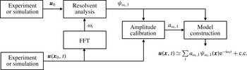
Figure 1 illustrates schematically the construction of the model employed to estimate the unsteady forces. The time mean flow
 $\boldsymbol{u}_{0}(\boldsymbol{x})$
and a pointwise measurement
 $\boldsymbol{u}(\boldsymbol{x}_{0},t)$
of the velocity history are the inputs, corresponding to the leftmost blocks. In principle, mean flow and probe information could be obtained independently from either experiments or simulations. A spectral analysis of the probe signal
 $\boldsymbol{u}(\boldsymbol{x}_{0},t)$
identifies the active frequencies
 $\unicode[STIX]{x1D714}_{i}$
to be explored in the resolvent analysis of the mean flow. The dominant resolvent modes
 $\unicode[STIX]{x1D713}_{\unicode[STIX]{x1D714}_{i},1}$
arising from the resolvent analysis corresponding to the active frequencies are calibrated with the probe signal to obtain the amplitude coefficients
 $a_{\unicode[STIX]{x1D714}_{i},1}$
. A linear combination of the weighted resolvent modes then provides an approximation of the fluctuating velocity and associated pressure fields.
Diagram of the construction of the model. The mean flow and pointwise measurement inputs are in the leftmost blocks. A fast Fourier transform (FFT) of the probe signal provides the active frequencies
 $\unicode[STIX]{x1D714}_{i}$
to be explored in the resolvent analysis of the mean flow. The dominant resolvent modes
 $\unicode[STIX]{x1D713}_{\unicode[STIX]{x1D714}_{i},1}$
corresponding to the active frequencies are calibrated with the probe signal to obtain the amplitude coefficients
 $a_{\unicode[STIX]{x1D714}_{i},1}$
. A linear combination of the weighted resolvent modes provides an approximation of the fluctuating velocity and pressure. The fluctuating pressure is included in the fluctuating velocity vector
 $\boldsymbol{u}=(u,v,w,p)^{\text{T}}$
for convenience.

2.1 Resolvent decomposition
We follow a similar derivation of the resolvent decomposition to that proposed by Luhar, Sharma & McKeon (Reference Luhar, Sharma and McKeon2014). This derivation differs from that by Gómez et al. (Reference Gómez, Blackburn, Rudman, Sharma and McKeon2016) in that the pressure is explicitly taken into account, instead of projecting the velocity onto a divergence-free basis. A Reynolds decomposition is applied to the total velocity
 $\hat{\boldsymbol{u}}(\boldsymbol{x},t)=\boldsymbol{u}_{0}(\boldsymbol{x})+\boldsymbol{u}(\boldsymbol{x},t)$
, with
 $\boldsymbol{u}(\boldsymbol{x},t)$
being the fluctuating velocity which may be decomposed as a sum of temporal Fourier modes
 $$\begin{eqnarray}\boldsymbol{u}(\boldsymbol{x},t)=\mathop{\sum }_{i}\boldsymbol{u}_{\unicode[STIX]{x1D714}_{i}}(\boldsymbol{x})\text{e}^{-\text{i}\unicode[STIX]{x1D714}_{i}t}.\end{eqnarray}$$
The flow is assumed to be statistically steady; thus, the frequencies
 $\unicode[STIX]{x1D714}_{i}$
are real. A similar decomposition may be applied to the nonlinear terms, leading to
 $\boldsymbol{f}_{\unicode[STIX]{x1D714}_{i}}=-(\boldsymbol{u}\boldsymbol{\cdot }\unicode[STIX]{x1D735}\boldsymbol{u})_{\unicode[STIX]{x1D714}_{i}}$
. These decompositions lead to a formulation of the Navier–Stokes equations as
 $$\begin{eqnarray}\displaystyle & \boldsymbol{u}_{0}\boldsymbol{\cdot }\unicode[STIX]{x1D735}\boldsymbol{u}_{0}=-\unicode[STIX]{x1D735}p+\mathit{Re}^{-1}\unicode[STIX]{x1D6FB}^{2}\boldsymbol{u}_{0}+\boldsymbol{f}_{0}, & \displaystyle\end{eqnarray}$$
 $$\begin{eqnarray}\displaystyle & \boldsymbol{u}_{\unicode[STIX]{x1D714}_{i}}=\mathscr{H}_{\unicode[STIX]{x1D714}_{i}}\boldsymbol{f}_{\unicode[STIX]{x1D714}_{i}}, & \displaystyle\end{eqnarray}$$
where
 $\mathscr{H}_{\unicode[STIX]{x1D714}_{i}}$
is the resolvent operator of the Navier–Stokes equations for each frequency
 $\unicode[STIX]{x1D714}_{i}$
. The mean flow equation (2.2) corresponds to
 $\unicode[STIX]{x1D714}=0$
and the Reynolds stress
 $\boldsymbol{f}_{0}$
denotes the interaction of the fluctuating velocity with the mean. The fluctuating pressure augments the fluctuating velocity vector as
 $\boldsymbol{u}=(u,v,w,p)^{\text{T}}$
, so the resolvent operator imposes the continuity equation
 $$\begin{eqnarray}\mathscr{H}_{\unicode[STIX]{x1D714}}=\left(-\text{i}\unicode[STIX]{x1D714}\left[\begin{array}{@{}cc@{}}\unicode[STIX]{x1D644} & 0\\ 0 & 0\end{array}\right]-\left[\begin{array}{@{}cc@{}}\mathscr{L} & -\unicode[STIX]{x1D735}\\ \unicode[STIX]{x1D735}^{\text{T}} & 0\end{array}\right]\right)^{-1}\left[\begin{array}{@{}cc@{}}\unicode[STIX]{x1D644} & 0\\ 0 & 0\end{array}\right],\end{eqnarray}$$
where
 $\mathscr{L}$
is the Jacobian of the Navier–Stokes equations and
 $\unicode[STIX]{x1D644}$
is an identity matrix. This operator represents how the fluctuating velocity
 $\boldsymbol{u}_{\unicode[STIX]{x1D714}}$
is driven by nonlinearity
 $\boldsymbol{f}_{\unicode[STIX]{x1D714}}$
in Fourier space; hence, it is useful to inspect its amplification properties via an SVD
 $$\begin{eqnarray}\mathscr{H}_{\unicode[STIX]{x1D714}}=\mathop{\sum }_{m}\unicode[STIX]{x1D74D}_{\unicode[STIX]{x1D714},m}\unicode[STIX]{x1D70E}_{\unicode[STIX]{x1D714},m}\unicode[STIX]{x1D753}_{\unicode[STIX]{x1D714},m}^{\ast },\end{eqnarray}$$
where
 $\unicode[STIX]{x1D74D}_{\unicode[STIX]{x1D714},m}$
and
 $\unicode[STIX]{x1D753}_{\unicode[STIX]{x1D714},m}$
are two orthonormal basis termed response and forcing modes respectively. The superscript
 $\ast$
indicates conjugate transpose and the subscript
 $m$
indicates the ordering of the modes, ranked by the amplification given by the corresponding singular value
 $\unicode[STIX]{x1D70E}_{\unicode[STIX]{x1D714},m}$
under the
 $L_{2}$
energy norm. The key of the resolvent decomposition is the projection on the nonlinearity onto the forcing modes (McKeon & Sharma Reference McKeon and Sharma2010). Hence, the fluctuating velocity can be written as a linear combination of response modes
 $$\begin{eqnarray}\boldsymbol{u}_{\unicode[STIX]{x1D714}}=\mathop{\sum }_{m}\unicode[STIX]{x1D74D}_{\unicode[STIX]{x1D714},m}\unicode[STIX]{x1D70E}_{\unicode[STIX]{x1D714},m}\unicode[STIX]{x1D712}_{\unicode[STIX]{x1D714},m},\end{eqnarray}$$
where the unknown scalar coefficients
 $\unicode[STIX]{x1D712}_{\unicode[STIX]{x1D714},m}$
are the projections of nonlinearity onto forcing modes and represent the forcing driving the velocity fluctuations (Gómez et al.
Reference Gómez, Blackburn, Rudman, Sharma and McKeon2016).
Equation (2.6) is an exact representation of the Navier–Stokes equation because no assumption other than a statistically steady flow has been used. On the other hand, it is useful to exploit the values taken by the amplification
 $\unicode[STIX]{x1D70E}_{\unicode[STIX]{x1D714},m}$
in order to construct a reduced-order model of the fluctuating velocity. In the presence of a single dominant flow feature such as a centrifugal instability (Gómez et al.
Reference Gómez, Blackburn, Rudman, Sharma and McKeon2016) or a critical layer response (McKeon & Sharma Reference McKeon and Sharma2010), the first singular value
 $\unicode[STIX]{x1D70E}_{\unicode[STIX]{x1D714},1}$
is usually much larger than the second one
 $\unicode[STIX]{x1D70E}_{\unicode[STIX]{x1D714},2}$
. Hence, at a particular frequency
 $\unicode[STIX]{x1D714}_{i}$
, irrespective of the values taken by
 $\unicode[STIX]{x1D712}_{\unicode[STIX]{x1D714},m}$
, it can be assumed that the projection of nonlinearity onto the first response
 $\unicode[STIX]{x1D74D}_{\unicode[STIX]{x1D714},1}$
is much larger than onto the rest. As such, the low-rank properties of the resolvent operator can be employed to yield a rank-1 model
 $$\begin{eqnarray}\boldsymbol{u}_{\unicode[STIX]{x1D714}}\simeq \unicode[STIX]{x1D74D}_{\unicode[STIX]{x1D714},1}a_{\unicode[STIX]{x1D714},1},\end{eqnarray}$$
where the amplitude coefficients
 $a_{\unicode[STIX]{x1D714},1}=\unicode[STIX]{x1D70E}_{\unicode[STIX]{x1D714},1}\unicode[STIX]{x1D712}_{\unicode[STIX]{x1D714},1}$
represent the amount of nonlinearity being amplified. Under this rank-1 assumption, the fluctuating velocity (and pressure) can be expressed as
 $$\begin{eqnarray}\boldsymbol{u}(\boldsymbol{x},t)\simeq \mathop{\sum }_{\unicode[STIX]{x1D714}}a_{\unicode[STIX]{x1D714},1}\unicode[STIX]{x1D74D}_{\unicode[STIX]{x1D714},1}(\boldsymbol{x})\text{e}^{-\text{i}\unicode[STIX]{x1D714}t}.\end{eqnarray}$$
Hence, this assumption provides a convenient model in which the velocity fluctuations at each frequency are parallel to the first singular response mode corresponding to that frequency. This rank-1 assumption has proven to be adequate in previous investigations of pipe, channel and cavity flows (McKeon & Sharma Reference McKeon and Sharma2010; Moarref et al. Reference Moarref, Sharma, Tropp and McKeon2013; Gómez et al. Reference Gómez, Blackburn, Rudman, Sharma and McKeon2016).
2.2 Amplitude calibration
It can be computationally challenging to obtain resolvent modes
 $\unicode[STIX]{x1D74D}_{\unicode[STIX]{x1D714},1}$
in complex three-dimensional geometries even using time-stepping methods. However, only a small number of modes corresponding to the relevant or active frequencies in the flow are computed in practice. In the absence of further information, the active frequencies of the flow are identified via a Fourier analysis of a pointwise measurement of the flow. As highlighted in figure 1, the probe information can be obtained independently of the mean flow. Here, we provide an extension of the calibration method developed by Gómez et al. (Reference Gómez, Blackburn, Rudman, Sharma and McKeon2016) to obtain the unknown amplitude coefficients that close the model (2.8) by using directly the same pointwise measurements of the velocity that have been previously employed for the identification of the active frequencies. At a particular spatial location
 $\boldsymbol{x}_{0}$
, the reduced-order model of the fluctuating velocity satisfies
 $$\begin{eqnarray}\boldsymbol{u}(\boldsymbol{x}_{0},t)\simeq \mathop{\sum }_{i=1}^{N_{\unicode[STIX]{x1D714}}}\unicode[STIX]{x1D74D}_{\unicode[STIX]{x1D714}_{i},1}(\boldsymbol{x}_{0})a_{\unicode[STIX]{x1D714}_{i},1}\text{e}^{-\text{i}\unicode[STIX]{x1D714}_{i}t},\end{eqnarray}$$
with
 $N_{\unicode[STIX]{x1D714}}$
representing the number of active frequencies (or discretized frequency bins) of the flow. Although each scalar component of (2.9) contains
 $N_{\unicode[STIX]{x1D714}}$
unknowns, it can be evaluated at a number of different time instants
 $N_{t}>N_{\unicode[STIX]{x1D714}}$
, such that the solution is amenable to a least-squares approximation. We note that the spatial structure of the fluctuating velocity is restricted by the response modes; hence, the pointwise calibration of the amplitude coefficients serves to capture the temporal behaviour of the fluctuating velocity. The solution of (2.9) in a least-squares sense is given by
 $$\begin{eqnarray}\boldsymbol{A}=\unicode[STIX]{x1D733}^{+}\boldsymbol{U}(\boldsymbol{x}_{\boldsymbol{ 0}},t),\end{eqnarray}$$
where the
 $3N_{t}\times N_{\unicode[STIX]{x1D714}}$
matrix
 $\unicode[STIX]{x1D733}$
contains the values of the three velocity components of the resolvent modes and their complex conjugates at the spatial location
 $\boldsymbol{x}_{0}$
at
 $N_{t}$
different times, the
 $N_{\unicode[STIX]{x1D714}}\times 1$
vector
 $\boldsymbol{A}$
represents the unknown amplitude coefficients and the
 $3N_{t}\times 1$
vector
 $\boldsymbol{U}$
contains the values of the velocity at the spatial location
 $\boldsymbol{x}_{0}$
at different times. The superscript
 $+$
denotes pseudoinverse. The dimensions of the least-squares problem (2.10) are much smaller than those of the SVD computations, and its solution is straightforward. Finally, the least-squares method employed to fit the amplitudes is optimal in minimizing the variance. Hence, in the case of Gaussian noise, the method would lead to a zero mean error. As such, sensor noise in the measurements would not be an issue for the present method.
3 Obtaining resolvent modes using time stepping
The most computationally demanding step in the creation of the model, depicted in figure 1, is obtaining the resolvent modes. As such, efficient methods to evaluate the resolvent operator are essential for the feasibility of the present methodology for the estimation of aerodynamic forces. We note from (2.4) that the resolvent operator can be evaluated via a shift and inversion of the Jacobian. Hence, matrix-free or matrix-forming methods, typically employed for global stability analysis (Paredes et al. Reference Paredes, Hermanns, Le Clainche and Theofilis2013), can be used to study the resolvent operator.
Although the simplest way to obtain the resolvent modes numerically is to assemble the resolvent operator and perform an SVD, this is difficult in practice due to the massive computational requirements resulting from the large dimensionality of the operator associated with flows with three non-homogeneous spatial directions. Thus, matrix-free methods are preferred for the study of these flows. In what follows, we describe a matrix-free methodology based on time stepping to obtain resolvent modes, potentially able to cope with three-dimensional flows.
The main idea of matrix-free methods is that the singular values of the resolvent operator are the eigenvalues of
 $\mathscr{H}_{\unicode[STIX]{x1D714}}\mathscr{H}_{\unicode[STIX]{x1D714}}^{\ast }$
, and the response and forcing singular vectors correspond to the eigenvectors of
 $\mathscr{H}_{\unicode[STIX]{x1D714}}\mathscr{H}_{\unicode[STIX]{x1D714}}^{\ast }$
and
 $\mathscr{H}_{\unicode[STIX]{x1D714}}^{\ast }\mathscr{H}_{\unicode[STIX]{x1D714}}$
respectively. As such, the action of the resolvent operator and its conjugate transpose on a forcing vector could enable a matrix-free iterative power method to obtain the SVD of
 $\mathscr{H}_{\unicode[STIX]{x1D714}}$
.
Following the rank-1 hypothesis posed in § 2.1, only the first singular vectors at each active frequency are required for the construction of the reduced-order model in (2.8). In this context, Monokrousos et al. (Reference Monokrousos, Åkervik, Brandt and Henningson2010) and Lu & Papadakis (Reference Lu and Papadakis2014) showed that obtaining the dominant singular vectors of the resolvent is equivalent to finding the optimal harmonic forcing of the forced linearized Navier–Stokes equations
 $$\begin{eqnarray}\unicode[STIX]{x2202}_{t}\boldsymbol{u}(\boldsymbol{x},t)=\mathscr{L}\boldsymbol{u}(\boldsymbol{x},t)+\boldsymbol{f}_{\unicode[STIX]{x1D714}}(\boldsymbol{x})\text{e}^{-\text{i}\unicode[STIX]{x1D714}t}.\end{eqnarray}$$
The long-time integration of (3.1) leads to the harmonic relation (2.3), if all transient effects vanish. Consequently, the optimal forcing and response vectors of
 $\mathscr{H}_{\unicode[STIX]{x1D714}}$
can be obtained from an optimization problem in a time-stepping context. A Lagrange function for the optimal forcing in (3.1) can be constructed as
 $$\begin{eqnarray}\boldsymbol{L}(\boldsymbol{u}_{\unicode[STIX]{x1D714}},\boldsymbol{f}_{\unicode[STIX]{x1D714}},\boldsymbol{v}_{\unicode[STIX]{x1D714}},\unicode[STIX]{x1D70E}^{2})=(\boldsymbol{u}_{\unicode[STIX]{x1D714}},\boldsymbol{u}_{\unicode[STIX]{x1D714}})-(\boldsymbol{v}_{\unicode[STIX]{x1D714}},(-\text{i}\unicode[STIX]{x1D714}\boldsymbol{I}-\mathscr{L}^{\ast })^{-1}\boldsymbol{u}_{\unicode[STIX]{x1D714}}-\boldsymbol{f}_{\unicode[STIX]{x1D714}})-\unicode[STIX]{x1D70E}_{\unicode[STIX]{x1D714}}^{2}((\boldsymbol{f}_{\unicode[STIX]{x1D714}},\boldsymbol{f}_{\unicode[STIX]{x1D714}})-1),\end{eqnarray}$$
where the objective function is the fluctuation energy represented by the energy norm
 $(\boldsymbol{u}_{\unicode[STIX]{x1D714}},\boldsymbol{u}_{\unicode[STIX]{x1D714}})$
. The first Lagrange multiplier
 $\boldsymbol{v}_{\unicode[STIX]{x1D714}}$
enforces that the response and forcing satisfy the forced linearized Navier–Stokes equations (3.1), and the second Lagrange multiplier
 $\unicode[STIX]{x1D70E}_{\unicode[STIX]{x1D714}}^{2}$
enforces a unit energy norm to the optimal forcing vector. Variations of
 $\boldsymbol{L}$
with respect to the fluctuating velocity
 $\boldsymbol{u}_{\unicode[STIX]{x1D714}}$
and to the forcing
 $\boldsymbol{f}_{\unicode[STIX]{x1D714}}$
yield respectively
 $$\begin{eqnarray}\displaystyle & \boldsymbol{v}_{\unicode[STIX]{x1D714}}=(-\text{i}\unicode[STIX]{x1D714}\unicode[STIX]{x1D644}-\mathscr{L}^{\ast })^{-1}\boldsymbol{u}_{\unicode[STIX]{x1D714}}, & \displaystyle\end{eqnarray}$$
 $$\begin{eqnarray}\displaystyle & \boldsymbol{f}_{\unicode[STIX]{x1D714}}=\boldsymbol{v}_{\unicode[STIX]{x1D714}}/\unicode[STIX]{x1D70E}_{\unicode[STIX]{x1D714}}^{2}. & \displaystyle\end{eqnarray}$$
The combination of the outcome of the optimization problem (3.3) and (3.4) with (2.3) leads to the eigenvalue problem
 $$\begin{eqnarray}\unicode[STIX]{x1D74D}_{\unicode[STIX]{x1D714},1}=\unicode[STIX]{x1D70E}_{\unicode[STIX]{x1D714},1}^{-2}(-\text{i}\unicode[STIX]{x1D714}\unicode[STIX]{x1D644}-\mathscr{L})^{-1}(\text{i}\unicode[STIX]{x1D714}\unicode[STIX]{x1D644}-\mathscr{L}^{\ast })^{-1}\unicode[STIX]{x1D74D}_{\unicode[STIX]{x1D714},1},\end{eqnarray}$$
where the fact that the optimal forcing solution corresponds to the first (most amplified) forcing mode
 $\unicode[STIX]{x1D74D}_{\unicode[STIX]{x1D714},1}$
has been exploited. An iterative matrix-free power method can be then applied to the eigenvalue problem (3.5) in order to obtain the dominant eigenvalue. However, as described by Monokrousos et al. (Reference Monokrousos, Åkervik, Brandt and Henningson2010), time stepping does not directly provide a solution of (2.3) or (3.3), and the forced linearized and adjoint equations need to be integrated for long enough such that the transient dynamics vanish and the response is harmonic. It should be noted that the long integration of the adjoint of (3.1),
 $$\begin{eqnarray}\unicode[STIX]{x2202}_{t}\boldsymbol{v}(\boldsymbol{x},t)=\mathscr{L}^{\ast }\boldsymbol{u}(\boldsymbol{x},t)+\boldsymbol{f}_{\unicode[STIX]{x1D714}}(\boldsymbol{x})\text{e}^{\text{i}\unicode[STIX]{x1D714}t},\end{eqnarray}$$
provides a harmonic solution for (3.3).
Although the algorithm originally proposed by Monokrousos et al. (Reference Monokrousos, Åkervik, Brandt and Henningson2010) is successful in the sense that it is matrix-free, a number of difficulties arise in practice. The time integration required of (3.1) until a harmonic response is obtained can be very long; hence, the method may not be computationally affordable. The method is particularly slow at low frequencies. Moreover, the complex velocity response
 $\boldsymbol{u}_{\unicode[STIX]{x1D714}}$
is obtained via a Fourier transform of
 $\boldsymbol{u}(t)$
during one period; hence, it could have a different phase at each iteration step. Finally, the response of (3.1) can be susceptible to large transient growths depending on the initial condition. Even if
 $\boldsymbol{u}_{\unicode[STIX]{x1D714}}$
and
 $\boldsymbol{f}_{\unicode[STIX]{x1D714}}$
are close to convergence, the transient can be significant if the two vectors do not have their relative phase fixed by the resolvent.
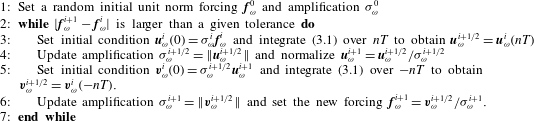
A modification of the time-stepping approach of Monokrousos et al. (Reference Monokrousos, Åkervik, Brandt and Henningson2010) that is able to cope with the abovementioned limitations is proposed by allowing the velocity field to take on complex values in the forced direct and adjoint linearized Navier–Stokes equations. The use of a complex variable has the advantage that it is not necessary to perform a Fourier transform of the response during one period to obtain
 $\boldsymbol{u}_{\unicode[STIX]{x1D714}}$
. Once the response of (3.1) is harmonic, any snapshot of the complex vector
 $\boldsymbol{u}^{\prime }(\boldsymbol{x},t)$
represents its Fourier transform
 $\boldsymbol{u}_{\unicode[STIX]{x1D714}}$
at some particular phase. Furthermore, if the time integration is taken as an integer number
 $n$
of periods
 $T=2\unicode[STIX]{x03C0}/\unicode[STIX]{x1D714}$
, the response and force vectors obtained remain with the same relative phase imposed by the resolvent during a complete iteration. This feature avoids possible sources of transient effects during iterations.
In addition, the integration time can be limited to a small number of periods
 $n$
such that the strongest transients have vanished but the flow is not yet exactly periodic. This permits an estimation of the amplification value and of the response and forcing vectors in relatively short integrals. The estimated
 $\unicode[STIX]{x1D70E}$
is then employed between each direct and adjoint iteration to successively generate a better initial condition at each iteration. As a result, the transient effects are damped and the harmonic response is achieved after a few iterations.
All of these features permit the most amplified modes to be obtained using a smaller computational effort than with the original algorithm of Monokrousos et al. (Reference Monokrousos, Åkervik, Brandt and Henningson2010). The modified algorithm is listed in table 1. In practice, the harmonic response is also assessed by monitoring the fluctuation energy. If the difference between the maximum and minimum fluctuation energies is less than a given tolerance within one period, the response is considered to be harmonic and the integration stops. Thus, each iteration may require a number of integration periods less than
 $n$
.
Time-stepping algorithm for computing resolvent modes in non-trivial domains.

3.1 Validation and comparison of the method
A validation of the computation of the resolvent modes via time stepping is carried out against results obtained using an in-house matrix-forming shift–invert method. The chosen validation case is the flow enclosed in a square lid-driven cavity at a Reynolds number based on lid length and speed
 $Re=1200$
with a periodic spanwise length
 $\unicode[STIX]{x1D6EC}=0.945$
(Gómez et al.
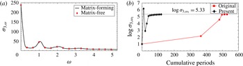
Reference Gómez, Blackburn, Rudman, Sharma and McKeon2016). A good agreement between the two methods is observed in figure 2(a). However, for the problem examined, while the matrix-forming approach requires the storage and evaluation of an
 $O(N^{2})$
matrix, the time-stepping approach only needs two planes with
 $O(N)$
degrees of freedom to deliver the same results. In the case presented, this evaluates to
 $3\times 64^{2}$
against
 $(3\times 64^{2})^{2}$
.
(a) Validation of the method: amplitude of the first resolvent modes in frequency at a spanwise wavenumber
 $\unicode[STIX]{x1D6FD}=3$
obtained with the matrix-forming and time-stepping matrix-free methods. (b) Comparison of the original time-stepping methods envisaged by Monokrousos et al. (Reference Monokrousos, Åkervik, Brandt and Henningson2010) and the present approach using
 $n=5$
: cumulative integration periods until convergence of the amplification. Symbols denote the estimated value at each iteration;
 $\unicode[STIX]{x1D6FD}=3$
,
 $\unicode[STIX]{x1D714}_{1}=5.26$
. The tolerance error is set to 0.005 and the two methods start with the same initial condition.

The optimal value of the parameter
 $n$
depends on the problem, and, for the present case, we have observed that the method typically converges in a few iterations using
 $n=5$
. In other words, five periods are sufficient to damp the most significant transient effects in the present case. Figure 2(b) shows a comparison of the present method with the original time-stepping methods envisaged by Monokrousos et al. (Reference Monokrousos, Åkervik, Brandt and Henningson2010). We observe that although the proposed methods requires a larger number of iterations, it needs significantly fewer integration periods to achieve convergence. In this example, the number of required integration periods until convergence goes from 540 periods to 116 periods, which translates into an
 ${\sim}80\,\%$
saving of CPU time.
4 Application to the flow around an inclined square cylinder
The flow past a two-dimensional inclined square cylinder may serve as a model for the flow around a non-trivial bluff body, and it is a good compromise between computational affordability and complex flow features (Sohankar, Norberg & Davidson Reference Sohankar, Norberg and Davidson1998; Yoon, Yang & Choi Reference Yoon, Yang and Choi2010). Beyond the critical Reynolds number, the wake becomes unsteady, presenting asymmetric vortex shedding; thus, this flow is interesting for the investigation of unsteady lift and drag forces.
Although the present methodology seems to be more appealing for experimental works, the mean flow and pointwise measure inputs to the model have been obtained via direct numerical simulation (DNS) using a spectral-element solver (Blackburn & Sherwin Reference Blackburn and Sherwin2004). A rectangular computational domain defined in
 $[-16,20]\times [-14,14]$
has been discretized with 236 spectral elements. The square cylinder has a unit side length and its centroid is located at
 $(x,y)=(0,0)$
. Temporal and spatial convergence has been achieved with a polynomial expansion of order 11 in each element and using a second-order temporal scheme with
 $\unicode[STIX]{x0394}t=8.5\times 10^{-3}$
. A constant velocity
 $(u,v)=(\cos \unicode[STIX]{x1D6FC},\sin \unicode[STIX]{x1D6FC})$
is imposed at the inlet of the domain, a no-slip boundary condition at the cylinder wall and Neumann boundary conditions at the outlet. The Reynolds number based on the cylinder side length
 $D$
and the modulus of the inlet velocity is fixed to
 $Re=100$
. The angle of attack is set to
 $\unicode[STIX]{x1D6FC}=10^{\circ }$
.
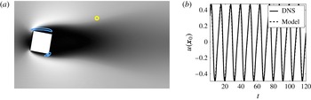
The inputs to the model corresponding to the leftmost block in figure 1 obtained via DNS, mean flow and a single pointwise measurement of the velocity are shown in figure 3. The probe is located at a random point in the wake of the cylinder where the shear is non-zero, and it serves to identify a single dominant frequency
 $\unicode[STIX]{x1D714}_{1}=0.908$
; hence, only one resolvent mode corresponding to that frequency needs to be computed. The dynamics of the self-interaction of this mode in this kind of flow could be relevant (Noack et al.
Reference Noack, Afanasiev, Morzyński, Tadmor and Thiele2003); thus, it may be convenient to also consider the first harmonic
 $\unicode[STIX]{x1D714}_{2}=2\unicode[STIX]{x1D714}_{1}$
, although in the present case the dynamics of the first harmonic does not show any significant influence on the aerodynamic forces, as will be shown.
The iterative time-stepping algorithm described in § 3 has been employed to obtain the two resolvent modes required to construct the reduced-order model. The forced linearized Navier–Stokes equations and their adjoint version have been solved with the same spectral-element solver as employed for DNS. The boundary conditions for each equation are described by Barkley, Blackburn & Sherwin (Reference Barkley, Blackburn and Sherwin2008); however, two sets of boundary conditions at the inlet have been tested for the forced adjoint equations: (i) an extended domain
 $[-40,20]\times [-14,14]$
with Dirichlet boundary conditions and (ii) the same domain as employed for the DNS with a non-physical forcing
 $-m(\boldsymbol{x})\boldsymbol{u}(\boldsymbol{x},t)$
applied at
 $-16<x<12$
to force a zero amplitude of the forcing mode at
 $x=-16$
. Both boundary conditions have provided similar results; thus, the former has been adopted on account of smaller computational requirements.
A comparison of the vorticity fields obtained from DNS and the resolvent-based model via calibration of the amplitude against the probe data in figure 3(b) is shown is figure 4. It is remarkable that the flow in the region around the cylinder, and hence the unsteady separation, is accurately predicted by the model, despite the probe being located approximately three side lengths from the cylinder. On the other hand, the structure of the wake far from the cylinder presents obvious discrepancies. Although the general feature of vortex shedding is also reproduced, the DNS presents additional features that the present resolvent-based model does not capture, like a consecutive and opposite vertical displacement of the vortex cores. An inspection of the spatial structure of the forcing mode that drives the resolvent modes, shown with blue isolines in figure 3(a), reveals that their maxima are located within the boundary layer of the cylinder; thus, the discrepancies between the model and the DNS can be attributed to this observation. As such, we presume that the additional dynamics of the far wake is governed by additional subdominant resolvent modes associated with the shear in the wake not considered in the present model.
Inputs to the model corresponding to the leftmost block in figure 1. (a) Streamwise velocity contours of the mean flow, coloured from black to white. Blue contour lines indicate 40 % and 80 % of the maximum of the kinetic energy corresponding to
 $\unicode[STIX]{x1D753}_{\unicode[STIX]{x1D714}_{1},1}$
. (b) Evolution of the fluctuating streamwise velocity in the wake at the location
 $\boldsymbol{x}_{0}=(3,1.5)$
, measured from the DNS and fitted to the model. The probe position is highlighted in (a) with a yellow circle.

Comparison of the fluctuating vorticity fields obtained from (a) DNS and (b) the resolvent-based model via calibration of the amplitude against the probe data in figure 3(b). The coloured contours represent
 $\pm 1/3$
of the maximum and minimum vorticity.

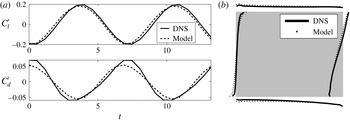
(a) Comparison of the temporal evolutions of the unsteady lift and drag coefficients calculated via DNS and predicted by the present methodology. (b) Representation of the fluctuating pressure distribution along the sides of the cylinder at a random instant calculated via DNS and predicted by the present methodology. Each cylinder side acts as an
 $x$
-axis, while its normal direction indicates the relative value of the unsteady pressure at that location.

The present approach is validated by measuring the unsteady lift and drag coefficients, defined as
 $$\begin{eqnarray}C_{l}^{\prime }=\int _{\unicode[STIX]{x1D6FF}\unicode[STIX]{x1D6FA}_{c}}p(\boldsymbol{x})\boldsymbol{n}\boldsymbol{\cdot }\boldsymbol{e}_{y},\quad C_{d}^{\prime }=\int _{\unicode[STIX]{x1D6FF}\unicode[STIX]{x1D6FA}_{c}}p(\boldsymbol{x})\boldsymbol{n}\boldsymbol{\cdot }\boldsymbol{e}_{x},\end{eqnarray}$$
where
 $\unicode[STIX]{x1D6FF}\unicode[STIX]{x1D6FA}_{c}$
denotes the boundary of the cylinder,
 $\boldsymbol{n}$
is the normal vector around the square cylinder, while
 $\boldsymbol{e}_{x}$
and
 $\boldsymbol{e}_{y}$
are the unit vectors in the streamwise and normal directions respectively. At the present value of
 $Re$
, the contributions of the viscous forces are negligible. Nevertheless, they could be taken into account using the present methodology. A good agreement between the temporal evolutions of the unsteady lift and drag coefficients calculated via DNS and predicted by the present methodology is shown in figure 5(a). This result is consistent with the accurate prediction by the model of the near field around the cylinder shown in figure 4. To provide further insight, the fluctuating pressure distribution along the sides of the cylinder at a random instant is represented in figure 5(b). The resemblance between the pressure distributions corresponding to the DNS and the resolvent-based model supports the good agreement between the temporal evolutions of the unsteady lift and drag forces. Finally, the same approach has been carried out using different pointwise measurements. As remarked by Gómez et al. (Reference Gómez, Blackburn, Rudman, Sharma and McKeon2016), similar results are obtained provided that the probe is always positioned at a location where the fluctuating velocity is significant. As such, care is needed in the selection of the probe locations. For example, a probe far from the wake would present a negligible fluctuating velocity or a probe in the wake centreline far from the cylinder would only show dynamics corresponding to the first harmonic frequency
 $\unicode[STIX]{x1D714}_{2}$
. However, this potential pitfall can be easily overcome by selecting more than one probe location, as shown by Gómez et al. (Reference Gómez, Blackburn, Rudman, Sharma and McKeon2016). Furthermore, the locations where the fluctuating velocity is significant can be inferred from the spatial structure of the resolvent modes.
5 Conclusions
A novel method to estimate unsteady aerodynamic coefficients via pointwise measurements has been presented. The methodology requires two inputs: (i) the mean flow and (ii) temporal information from a probe. In principle, both inputs could be obtained either simultaneously or independently. Although we believe that the present methodology is more appealing for experimental investigations, e.g. using planar time-resolved PIV to obtain a three-dimensional mean flow and obtain temporal information at different locations, DNS was employed in the present work to obtain the mean flow and the pointwise data.
The most challenging step of the methodology is the computation of the resolvent modes. For this purpose, a computationally affordable time-stepping methodology to obtain resolvent modes of complex flows has been introduced, validated and compared with previous existing matrix-free and matrix-forming strategies.
The potential of the present methodology has been demonstrated by application to an unsteady two-dimensional flow around an inclined square cylinder at low Reynolds number. The present approach can predict the fluctuating velocity associated with unsteady separation and the pressure distribution near the square cylinder using just the leading response mode. The temporal evolutions of the lift and drag coefficients computed from these fields are in good agreement with those obtained via DNS.
Acknowledgements
The authors acknowledge financial support from the Australian Research Council through grant DP130103103, and from Australia’s National Computational Infrastructure via Merit Allocation Scheme grant D77.