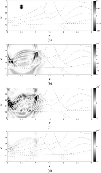
1. Introduction
The present article is motivated by the recent successes of radial basis functions (RBFs) in the field of computational geoscience. This is quite far from how the RBF methodology first originated. It was proposed by Hardy (Reference Hardy1971) in connection with a cartography application that required multivariate scattered-node interpolation. A key non-singularity proof by Micchelli (Reference Micchelli1986) accelerated the further development and acceptance of RBFs. Pioneering work by Powell (Reference Powell and Light1992) and his collaborators at the University of Cambridge also played a major role in the early history of RBFs. Kansa (Reference Kansa1990a , Reference Kansa1990b ) suggested that taking analytic derivatives of RBF interpolants could provide a numerical solution approach for PDEs.
Several monographs on RBFs or with extensive RBF content appeared between 2003 and 2007, by Buhmann (Reference Buhmann2003), Iske (Reference Iske2004), Wendland (Reference Wendland2005) and Fasshauer (Reference Fasshauer2007). Acta Numerica has featured two RBF articles, Buhmann (Reference Buhmann2000) and Schaback and Wendland (Reference Schaback and Wendland2006). These works reflected a growing use of RBFs as a practical computational procedure for increasingly larger-scale applications. Like Fasshauer (Reference Fasshauer2007), the brief monograph by Chen, Fu and Chen (Reference Chen, Fu and Chen2014) discussed certain RBF approaches for solving PDEs. The perspective presented in this article – as well as in the forthcoming SIAM monograph by Fornberg and Flyer (Reference Fornberg and Flyer2015b ) – is quite different, and will also describe the RBF-FD (RBF-generated finite difference) approach.
We will omit quite large areas of RBF theory that are well described in the previous monographs, and in particular results that are not directly needed for effectively solving PDEs. Attention will, however, be given to ‘flat’ (or near-flat) basis functions, to the use of RBFs for creating weights for RBF-FD formulas, and to the application of RBF/RBF-FD discretizations for solving large-scale benchmark problems, mostly from the geosciences.
2. Background to RBFs for PDEs
PDE discretizations in more than one dimension are often based on meshes, which may be either structured or unstructured, with the latter case best known in the context of finite elements. In the former case, it is relatively easy to approximate derivatives to high orders of accuracy by making finite difference (FD) stencils increasingly wide. That limit provides an alternative way to understand and use pseudospectral (PS) methods (Boyd Reference Boyd2000, Fornberg Reference Fornberg1996, Trefethen Reference Trefethen2000). A more common way to implement PS methods is via expansions in basis functions, such as tensor products of one-dimensional Fourier or Chebyshev expansions. The computational efficiency of the resulting procedure can in some cases become very high, but this comes at the price of severe regularity constraints on the shape of the computational domain. Spectral element approaches, involving domain decomposition into rectangles (when in two dimensions), together with curvilinear mappings can overcome some of this, and can also permit local refinement in critical areas. However, their implementation is complex and the small node spacing that becomes necessary near internal (artificial) boundaries often severely hurts time-stepping stability conditions.
When solving PDEs, it is very desirable to use entirely mesh-free node distributions, that is, to be able to scatter computational nodes (collocation points) just as needed to fit boundaries and to satisfy spatially variable resolution requirements, but without having to form any local triangles or tetrahedra. Furthermore, with a derivative being a local property of a function, it makes sense to rely on spatially localized approximations. While global approximations can have high formal orders of accuracy, their cost is typically high. This is due both to high operation counts and to costly data flow on modern computers with hierarchical memory structures.
Historically, one can recognize an evolutionary path
 $\text{FD}\Rightarrow \text{PS}\Rightarrow \text{RBF}\Rightarrow \text{RBF-FD}$
that starts by extending from FD methods (first applied to PDEs just over a century ago: see Richardson Reference Richardson1911) to PS methods. It transpires that each PS method can be seen as a special case of an RBF approximation in a certain limit. With the RBF representation, geometric flexibility has been achieved. When RBFs are then used to create weights for scattered-node FD-like stencils (i.e., RBF-FD approximations), approximations have again become ‘local’, with associated high computational speeds and excellent scaling properties for massively large problem sizes.
Concerning interpolation over scattered nodes, using standard basis functions, the following theorem may at first appear discouraging.
Mairhuber–Curtis theorem (Curtis Reference Curtis1959, Mairhuber Reference Mairhuber1956). Given any set of basis functions
 $\{F_{k}(\mathbf{x}),k=1,2,\ldots ,N\}$
with
 $\mathbf{x}\in R^{d},d\geq 2$
, the problem of determining an interpolant
 $$\begin{eqnarray}s(\mathbf{x})=\mathop{\sum }_{k=1}^{N}{\it\lambda}_{k}F_{k}(\mathbf{x}),\end{eqnarray}$$
satisfying
 $s(\mathbf{x}_{k})=f_{k}$
, is singular for infinitely many configurations of distinct nodes
 $\mathbf{x}_{k},k=1,2,\ldots ,N$
.
Proof. The interpolation requirement
 $s(\mathbf{x}_{k})=f_{k}$
implies that the coefficients
 ${\it\lambda}_{k}$
in (2.1) will satisfy the linear system
 $$\begin{eqnarray}\left[\begin{array}{@{}cccc@{}}F_{1}(\mathbf{x}_{1}) & F_{2}(\mathbf{x}_{1}) & \cdots \, & F_{N}(\mathbf{x}_{1})\\ F_{1}(\mathbf{x}_{2}) & F_{2}(\mathbf{x}_{2}) & \cdots \, & F_{N}(\mathbf{x}_{2})\\ \vdots & \vdots & & \vdots \\ F_{1}(\mathbf{x}_{N}) & F_{2}(\mathbf{x}_{N}) & \cdots \, & F_{N}(\mathbf{x}_{N})\end{array}\right]\left[\begin{array}{@{}c@{}}{\it\lambda}_{1}\\ {\it\lambda}_{2}\\ \vdots \\ {\it\lambda}_{N}\end{array}\right]=\left[\begin{array}{@{}c@{}}f_{1}\\ f_{2}\\ \vdots \\ f_{N}\end{array}\right].\end{eqnarray}$$
In more than one dimension, it is possible to move the nodes continuously so that two nodes end up interchanged, without them having coincided at any time. The effect on the coefficient matrix in (2.2) is that two rows have become interchanged, that is, its determinant has changed sign. By continuity, the determinant must therefore have been zero somewhere along the way.☐
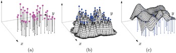
The consequence of the theorem above is that vast numbers of seemingly ‘innocent’ node configurations will give rise to singular systems. The RBF idea for overcoming this issue is sketched in Figure 2.1. The basis functions are radially symmetric here, typically with one centred at each node point
 $\mathbf{x}_{k}$
, that is, of the form
 ${\it\phi}(\Vert \mathbf{x}-\mathbf{x}_{k}\Vert )$
. Here
 ${\it\phi}$
is a radial function (such as
 ${\it\phi}(r=\Vert \mathbf{x}-\mathbf{x}_{k}\Vert )=\text{e}^{-({\it\varepsilon}r)^{2}}$
),
 ${\it\varepsilon}$
is a shape parameter, and the norm is the standard Euclidean distance function. Again, letting the data value be
 $f_{k}$
at node
 $\mathbf{x}_{k},k=1,2,\ldots ,N$
, the coefficients in the RBF interpolant of
 $f(\mathbf{x})$
,
 $$\begin{eqnarray}s(\mathbf{x})=\mathop{\sum }_{k=1}^{N}{\it\lambda}_{k}{\it\phi}(\Vert \mathbf{x}-\mathbf{x}_{k}\Vert ),\end{eqnarray}$$
can be found by solving a system very similar to (2.2):
 $$\begin{eqnarray}\hspace{-2.0pt}\left[\begin{array}{@{}cccc@{}}{\it\phi}(\Vert \mathbf{x}_{1}-\mathbf{x}_{1}\Vert )\! & {\it\phi}(\Vert \mathbf{x}_{1}-\mathbf{x}_{2}\Vert ) & \!\!\cdots \!\! & {\it\phi}(\Vert \mathbf{x}_{1}-\mathbf{x}_{N}\Vert )\\ {\it\phi}(\Vert \mathbf{x}_{2}-\mathbf{x}_{1}\Vert )\! & {\it\phi}(\Vert \mathbf{x}_{2}-\mathbf{x}_{2}\Vert ) & \!\!\cdots \!\! & {\it\phi}(\Vert \mathbf{x}_{2}-\mathbf{x}_{N}\Vert )\\ \vdots & \vdots & & \vdots \\ {\it\phi}(\Vert \mathbf{x}_{N}-\mathbf{x}_{1}\Vert )\! & {\it\phi}(\Vert \mathbf{x}_{N}-\mathbf{x}_{2}\Vert ) & \!\!\cdots \!\! & {\it\phi}(\Vert \mathbf{x}_{N}-\mathbf{x}_{N}\Vert )\end{array}\right]\left[\begin{array}{@{}c@{}}{\it\lambda}_{1}\\ {\it\lambda}_{2}\\ \vdots \\ {\it\lambda}_{N}\end{array}\right]=\left[\begin{array}{@{}c@{}}f_{1}\\ f_{2}\\ \vdots \\ f_{N}\end{array}\right]\!.\end{eqnarray}$$
Moving two nodes so that they change places again interchanges two rows but now also two columns, leaving the sign of the determinant unaffected. Therefore, the singularity argument above no longer applies. The key difference from the assumptions in the Mairhuber–Curtis theorem is that the basis functions
 ${\it\phi}(\Vert \mathbf{x}-\mathbf{x}_{k}\Vert )$
depend on the node locations.
Graphical illustration of the RBF concept. (a) Example of two-dimensional scattered data. (b) Basis function set. One rotated Gaussian is located at each data point. (c) The unique linear combination of the Gaussians that agrees with all the provided data.

2.1. Different RBF types
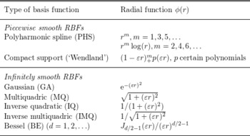
Table 2.1 lists a number of RBF types. For most of these, we will show in Section 2.2 that the system (2.4) can never be singular, for any number of (distinct) nodes scattered in any number of dimensions.
Some common choices for radial functions.

2.1.1. Piecewise smooth RBFs
The listed ‘piecewise smooth’ radial functions will cause a singularity at the origin of the associated RBF and, in the compactly supported ‘Wendland’ case, also at
 $r=1/{\it\varepsilon}$
. This is entirely acceptable in many applications, but puts them at a disadvantage in other cases, such as when seeking accurate solutions to convection-type PDEs over long times (Fornberg and Piret Reference Fornberg and Piret2008). The property of compactly supported RBFs to produce sparse rather than full linear systems is advantageous in some contexts such as image rendering, but less so when approximating PDEs, since the differentiation matrices that result from them nevertheless become full matrices.
PHS-type RBFs are associated with several optimality results, such as interpolating scattered data with the least possible overall curvature (Duchon Reference Duchon, Schempp and Zeller1977, Powell Reference Powell and Light1992). They are also of particular interest in the context of RBF-FD.
It can be noted that
 ${\it\phi}(r)=r^{3}$
in one dimension reproduces cubic splines, albeit with highly unusual end conditions. With slight modifications in the form of (2.3), one can, however, obtain either ‘natural’ or ‘not-a-knot’ splines. Similar modifications can also be applied to other RBF types and for scattered nodes in higher dimensions, offering easy-to-apply approaches for enhancing the accuracy at domain boundaries (Fornberg, Driscoll, Wright and Charles Reference Fornberg, Driscoll, Wright and Charles2002).
2.1.2. Infinitely smooth RBFs
As noted above,
 ${\it\phi}(r)=r^{3}$
in one dimension leads to a cubic spline, featuring a jump in the third derivative at each node. Disregarding possible boundary effects, its accuracy is well known to be
 $O(h^{4})$
on a grid with spacing
 $h$
. Similarly,
 ${\it\phi}(r)=r^{5}$
leads to
 $O(h^{6})$
-errors, etc. This raises the obvious question why one would use radial functions that cause jumps in any derivative. For the infinitely smooth ones, there are no such jumps, and that suffices to obtain spectral accuracy – better than any algebraic order
 $O(h^{p}),$
 $p\in \mathbb{N}$
, assuming that no counterpart to the polynomial Runge phenomenon arises (Madych and Nelson Reference Madych and Nelson1992).
All smooth radial functions (of which there are many more options than are listed in Table 2.1) feature a shape parameter, denoted by
 ${\it\varepsilon}$
. While one could also apply an
 ${\it\varepsilon}$
-scaling to the PHS functions, such as
 ${\it\phi}(r)=r^{m},$
that is, use
 ${\it\phi}(r)=({\it\varepsilon}r)^{m},$
this would serve no purpose since
 $({\it\varepsilon}r)^{m}={\it\varepsilon}^{m}r^{m}$
, and the scale factor would then vanish analytically by the time the interpolant
 $s(\mathbf{x})$
is obtained.
2.2. Non-singularity theorems
Following Bochner (Reference Bochner1933), we will first show that the RBF matrix
 $$\begin{eqnarray}A=\left[\begin{array}{@{}cccc@{}}{\it\phi}(\Vert \mathbf{x}_{1}-\mathbf{x}_{1}\Vert ) & {\it\phi}(\Vert \mathbf{x}_{1}-\mathbf{x}_{2}\Vert ) & \cdots \, & {\it\phi}(\Vert \mathbf{x}_{1}-\mathbf{x}_{N}\Vert )\\ {\it\phi}(\Vert \mathbf{x}_{2}-\mathbf{x}_{1}\Vert ) & {\it\phi}(\Vert \mathbf{x}_{2}-\mathbf{x}_{2}\Vert ) & \cdots \, & {\it\phi}(\Vert \mathbf{x}_{2}-\mathbf{x}_{N}\Vert )\\ \vdots & \vdots & & \vdots \\ {\it\phi}(\Vert \mathbf{x}_{N}-\mathbf{x}_{1}\Vert ) & {\it\phi}(\Vert \mathbf{x}_{N}-\mathbf{x}_{2}\Vert ) & \cdots \, & {\it\phi}(\Vert \mathbf{x}_{N}-\mathbf{x}_{N}\Vert )\end{array}\right]\end{eqnarray}$$
is guaranteed to be non-singular for GA RBFs, no matter how the nodes (assumed to be distinct) are scattered in any number of dimensions. This result will then be generalized to several other RBF types.
2.2.1. Gaussian RBFs
A real symmetric matrix
 $A$
is positive definite if and only if
 ${\bf\alpha}^{T}A{\bf\alpha}>0$
for every real vector
 ${\bf\alpha}\neq \mathbf{0}$
. All eigenvalues are then positive, and the matrix will be non-singular. The proof that the
 $A$
-matrix for GA RBFs is positive definite can be carried out in three steps.
Step 1: Recall the Fourier transform of Gaussians. We define the one-dimensional Fourier transform (FT) as
 $$\begin{eqnarray}\displaystyle u(x) & = & \displaystyle {\displaystyle \frac{1}{\sqrt{2{\it\pi}}}}\int _{-\infty }^{\infty }\widehat{u}({\it\omega})\;\text{e}^{\text{i}{\it\omega}x}\,\text{d}{\it\omega},\nonumber\\ \displaystyle \widehat{u}({\it\omega}) & = & \displaystyle {\displaystyle \frac{1}{\sqrt{2{\it\pi}}}}\int _{-\infty }^{\infty }u(x)\;\text{e}^{-\text{i}{\it\omega}x}\,\text{d}x.\nonumber\end{eqnarray}$$
Applying the one-dimensional result
 $$\begin{eqnarray}u(x)=\text{e}^{-{\it\varepsilon}^{2}x^{2}}\Leftrightarrow \widehat{u}({\it\omega})=\frac{1}{\sqrt{2}{\it\varepsilon}}\;\text{e}^{-{\it\omega}^{2}/(4{\it\varepsilon}^{2})}\end{eqnarray}$$
 $d$
times, we obtain the
 $d$
-dimensional case
 $$\begin{eqnarray}u(\mathbf{x})=\text{e}^{-{\it\varepsilon}^{2}\Vert \mathbf{x}\Vert ^{2}}\Leftrightarrow \widehat{u}({\bf\omega})=\frac{1}{2^{d/2}{\it\varepsilon}^{d}}\;\text{e}^{-\Vert {\bf\omega}\Vert ^{2}/(4{\it\varepsilon}^{2})}.\end{eqnarray}$$
Inverting
 $\widehat{u}({\bf\omega})$
back to physical space produces the identity
 $$\begin{eqnarray}\text{e}^{-{\it\varepsilon}^{2}\Vert \mathbf{x}\Vert ^{2}}=\frac{1}{(2{\it\pi})^{d/2}}\int _{R^{d}}\frac{1}{2^{d/2}{\it\varepsilon}^{d}}\text{e}^{-\Vert {\bf\omega}\Vert ^{2}/(4{\it\varepsilon}^{2})}\;\text{e}^{\text{i}\;\mathbf{x}\cdot {\bf\omega}}\,\text{d}{\bf\omega}.\end{eqnarray}$$
It may at first seem that this way to rewrite the GA radial function
 $\text{e}^{-{\it\varepsilon}^{2}\Vert \mathbf{x}\Vert ^{2}}$
has introduced a lot of extra complexity. However, the key point will turn out to be that
 $\mathbf{x}$
, appearing quadratically as
 $\Vert \mathbf{x}\Vert ^{2}$
in the exponent in the left-hand side, appears only linearly, as
 $\mathbf{x}$
, in one of the exponents in the right-hand side.
Step 2: Proof that A is positive semidefinite. Let
 $$\begin{eqnarray}{\bf\alpha}\;=[{\it\alpha}_{1},\ldots ,{\it\alpha}_{N}]^{T}\neq \mathbf{0}.\end{eqnarray}$$
Then
 $$\begin{eqnarray}\displaystyle {\bf\alpha}^{T}A\;{\bf\alpha} & = & \displaystyle \mathop{\sum }_{j=1}^{N}\mathop{\sum }_{k=1}^{N}{\it\alpha}_{j}{\it\alpha}_{k}\text{e}^{-{\it\varepsilon}^{2}\Vert \mathbf{x}_{j}-\mathbf{x}_{k}\Vert ^{2}}\quad \text{(apply (2.7))}\nonumber\\ \displaystyle & = & \displaystyle \mathop{\sum }_{j=1}^{N}\mathop{\sum }_{k=1}^{N}{\it\alpha}_{j}{\it\alpha}_{k}\frac{1}{(2{\it\pi})^{d/2}}\int _{R^{d}}\frac{1}{(2{\it\varepsilon}^{2})^{d/2}}\text{e}^{-\Vert {\bf\omega}\Vert ^{2}/(4{\it\varepsilon}^{2})}\;\text{e}^{\text{i}\,(\mathbf{x}_{j}-\mathbf{x}_{k})\cdot {\bf\omega}}\,\text{d}{\bf\omega}\nonumber\\ \displaystyle & = & \displaystyle \frac{1}{(2{\it\varepsilon})^{d}{\it\pi}^{d/2}}\int _{R^{d}}\text{e}^{-\Vert {\bf\omega}\Vert ^{2}/(4{\it\varepsilon}^{2})}\left(\mathop{\sum }_{j=1}^{N}\mathop{\sum }_{k=1}^{N}{\it\alpha}_{j}{\it\alpha}_{k}\;\text{e}^{\text{i}\,(\underline{x}_{j}-\underline{x}_{k})\cdot {\bf\omega}}\right)\,\text{d}{\bf\omega}.\nonumber\end{eqnarray}$$
The double sum inside the integral can be written as
 $$\begin{eqnarray}\left(\mathop{\sum }_{j=1}^{N}{\it\alpha}_{j}\;\text{e}^{\text{i}\mathbf{x}_{j}\cdot {\bf\omega}}\right)\overline{\left(\mathop{\sum }_{k=1}^{N}{\it\alpha}_{k}\;\text{e}^{\text{i}\mathbf{x}_{k}\cdot {\bf\omega}}\right)}=\Vert \mathop{\sum }_{m=1}^{N}{\it\alpha}_{m}\;\text{e}^{\text{i}\mathbf{x}_{m}\cdot {\bf\omega}}\Vert ^{2}\geq 0.\end{eqnarray}$$
Thus
 ${\bf\alpha}^{T}A\;{\bf\alpha}\geq 0$
, and we have shown that the matrix
 $A$
is positive semidefinite.
Step 3: Proof that A is positive definite. Based on the result above, it only remains to show that
 $$\begin{eqnarray}\mathop{\sum }_{m=1}^{N}{\it\alpha}_{m}\;\text{e}^{\text{i}\,\mathbf{x}_{m}\cdot {\bf\omega}}\end{eqnarray}$$
cannot be identically zero (as a function of
 $\boldsymbol{{\bf\omega}}$
) unless all the coefficients
 ${\it\alpha}_{m}$
are zero. Several different short proofs for this are available (Fasshauer Reference Fasshauer2007, Fornberg and Flyer Reference Fornberg and Flyer2015b
, Powell Reference Powell and Light1992).
2.2.2. Some other RBF types
If (2.6) is replaced by
 $$\begin{eqnarray}u(\mathbf{x})=f({\it\varepsilon}\Vert \mathbf{x}\Vert )\Leftrightarrow \widehat{u}({\bf\omega})=g(\Vert {\bf\omega}\Vert /{\it\varepsilon})\end{eqnarray}$$
with
 $g(\Vert {\bf\omega}\Vert )>0$
, the replacement for the leading factor
 $(\text{e}^{-\Vert {\bf\omega}\Vert ^{2}/(4{\it\varepsilon}^{2})})$
inside the integral in (2.7) will again be positive, and the positive definiteness proof will carry through just as in the GA case. This situation arises for many types of compactly supported RBFs, for example.
Another variation of the non-singularity proof (related to the theory of completely monotone functions: Schoenberg Reference Schoenberg1938), proceeds as follows. Taking the inverse Laplace transform of
 ${\it\phi}(\sqrt{r})$
for different radial functions
 ${\it\phi}(r)$
gives formulas such as
 $$\begin{eqnarray}\displaystyle \begin{array}{@{}ll@{}}\text{IQ} & \displaystyle {\displaystyle \frac{1}{1+({\it\varepsilon}r)^{2}}}=\int _{0}^{\infty }\text{e}^{-s}\text{e}^{-s({\it\varepsilon}r)^{2}}\,\text{d}s,\\ \text{IMQ} & \displaystyle {\displaystyle \frac{1}{\sqrt{1+({\it\varepsilon}r)^{2}}}}=\int _{0}^{\infty }{\displaystyle \frac{\text{e}^{-s}}{\sqrt{{\it\pi}s}}}\text{e}^{-s({\it\varepsilon}r)^{2}}\,\text{d}s.\end{array} & & \displaystyle \nonumber\end{eqnarray}$$
In all cases when the factor in front of
 $\text{e}^{-s({\it\varepsilon}r)^{2}}$
inside the integral is positive, we observe that (using IQ as an illustration)
 $$\begin{eqnarray}\displaystyle {\bf\alpha}^{T}A{\bf\alpha} & = & \displaystyle \mathop{\sum }_{j=1}^{N}\mathop{\sum }_{k=1}^{N}{\it\alpha}_{j}{\it\alpha}_{k}\frac{1}{1+{\it\varepsilon}^{2}\Vert \mathbf{x}_{j}-\mathbf{x}_{k}\Vert ^{2}}\nonumber\\ \displaystyle & = & \displaystyle \int _{0}^{\infty }\text{e}^{-s}\left(\mathop{\sum }_{j=1}^{N}\mathop{\sum }_{k=1}^{N}{\it\alpha}_{j}{\it\alpha}_{k}\text{e}^{-s\;{\it\varepsilon}^{2}\Vert \mathbf{x}_{j}-\mathbf{x}_{k}\Vert ^{2}}\right)\,\text{d}s.\nonumber\end{eqnarray}$$
From the non-singularity proof for GA RBFs, we know that the double sum is positive whenever the vector
 ${\bf\alpha}=[{\it\alpha}_{1},{\it\alpha}_{2},\ldots ,{\it\alpha}_{N}]^{T}$
is not identically zero. Therefore, the integral and thus the quantity
 ${\bf\alpha}^{T}A{\bf\alpha}$
will also be positive, that is,
 $A$
is a positive definite matrix.
The proofs above do not directly apply to the commonly used MQ case. It transpires, however, that non-singularity is again assured, with the (symmetric) A-matrix now having one positive eigenvalue and all the remaining ones negative. The original proof by Micchelli (Reference Micchelli1986) was later simplified in Powell (Reference Powell2005).
3. Near-flat RBFs
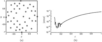
(a) A set of 41 scattered nodes in the unit circle. (b) The error in the max norm when the test function
 $f(x,y)=59/(67+(x+\frac{1}{7})^{2}+(y-\frac{1}{11})^{2})$
is interpolated using these nodes, displayed as a function of the shape parameter
 ${\it\varepsilon}$
.

With
 ${\it\varepsilon}$
available as a free parameter, it is natural to explore how the choice of
 ${\it\varepsilon}$
influences the accuracy obtained. A typical test is shown in Figure 3.1. As first noted by Tarwater (Reference Tarwater1985), it often happens that the error decreases rapidly with
 ${\it\varepsilon}$
until the calculation suddenly breaks down due to the increasing ill-conditioning of the linear system (2.4). This may suggest that a trade-off will be required between accuracy and numerical conditioning (described as an ‘uncertainty principle’ in Schaback Reference Schaback1995). It was soon realized, however, that the RBF interpolation problem actually does not become ill-conditioned in this flat basis function limit, and that the apparent problem was particular to the RBF-Direct procedure: solution of (2.4) followed by evaluation of (2.3). RBF-Direct uses ill-conditioned expansion coefficients
 ${\it\lambda}_{k}$
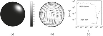
as intermediate quantities for arriving at what should be a well-conditioned result (Driscoll and Fornberg Reference Driscoll and Fornberg2002, Fornberg, Wright and Larsson Reference Fornberg, Wright and Larsson2004). Several well-conditioned stable numerical algorithms were subsequently developed (see Section 3.2), giving results as seen in one typical case in Figure 3.2. Sometimes, the most accurate
 ${\it\varepsilon}$
-range can be reached with RBF-Direct. In other cases, such as the one illustrated here, this requires a stable algorithm.
If the nodes are lattice-based, it can happen that the RBF interpolant diverges when
 ${\it\varepsilon}\rightarrow 0$
(Fornberg, Larsson and Wright Reference Fornberg, Larsson and Wright2006, Fornberg and Wright Reference Fornberg and Wright2004), although never in the GA case (Schaback Reference Schaback2005), a fact that contributes to making GA a popular RBF choice. For node sets with some irregularity, the interpolant will in the flat
 ${\it\varepsilon}\rightarrow 0$
limit take the form of a multivariate polynomial (Driscoll and Fornberg Reference Driscoll and Fornberg2002, Fornberg et al.
Reference Fornberg, Wright and Larsson2004). One reason that small
 ${\it\varepsilon}$
is often better than
 ${\it\varepsilon}\rightarrow 0$
is that, with RBF interpolants converging to polynomials, the boundary accuracy often deteriorates due to the Runge phenomenon (Fornberg and Zuev Reference Fornberg and Zuev2007). In the high-degree polynomial case, Chebyshev-style node clustering near the boundaries is the most frequently used remedy (in spite of disadvantages, such as causing adverse stability conditions in the context of explicit time-stepping of PDEs). As was noted in Section 2.1.1, a number of additional options are available for RBFs.
(a) Test function
 $f(x)=\exp (-7(x+{\textstyle \frac{1}{2}})^{2}-8(y+{\textstyle \frac{1}{2}})^{2}-9(z-{\textstyle \frac{1}{\sqrt{2}}})^{2}).$
(b)
 $N=1849$
ME (minimal energy) nodes on the surface of the unit sphere. (c) MQ interpolation errors (in the max norm), as functions of
 ${\it\varepsilon}$
, when using RBF-Direct versus using the stable RBF-QR algorithm. The RBF-QR error level seen here for small
 ${\it\varepsilon}$
is unrelated to the nearby machine rounding level of
 $10^{-16}$
.

3.1. The ill-conditioning of the
 $A$
-matrix

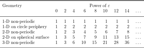
Sideways translates of near-flat basis functions all look the same, and it is intuitively obvious that they must form a very ill-conditioned base to expand in. Just how bad it is can readily be quantified (Fornberg and Zuev Reference Fornberg and Zuev2007). For example, when using infinitely smooth RBFs on scattered nodes in two dimensions, the eigenvalues of the
 $A$
-matrix form distinct groups, following the specific pattern
 $$\begin{eqnarray}\begin{array}{@{}l@{}}\{O(1)\},\\ \{O({\it\varepsilon}^{2}),O({\it\varepsilon}^{2})\},\\ \{O({\it\varepsilon}^{4}),O({\it\varepsilon}^{4}),O({\it\varepsilon}^{4})\},\\ \{O({\it\varepsilon}^{6}),O({\it\varepsilon}^{6}),O({\it\varepsilon}^{6}),O({\it\varepsilon}^{6})\},\\ \cdots \end{array}\end{eqnarray}$$
until the last eigenvalue is reached, causing the last group to possibly contain fewer eigenvalues than the general pattern would suggest. Different choices of scattered-node locations or of RBF types (IQ, MQ, or GA), make no difference in this regard. However, use of lattice-based nodes or Bessel-type RBFs result in exceptions (with smaller groups, implying worse conditioning). More concisely, we can write the eigenvalue pattern above as
 $$\begin{eqnarray}1,2,3,4,\ldots ,\end{eqnarray}$$
indicating how many eigenvalues there are of orders
 ${\it\varepsilon}^{0},{\it\varepsilon}^{2},{\it\varepsilon}^{4},{\it\varepsilon}^{6},$
etc. Table 3.1 shows some more such sequences. The patterns are readily recognizable: for example, in the
 $d$
-dimensional non-periodic case, the
 $k$
th entry is
 $\binom{d+k-2}{k-1}$
. Given these patterns, one can immediately calculate the orders of both
 $\text{cond}(A)$
and
 $\det (A)=\prod _{k=1}^{n}{\it\lambda}_{k}$
as functions of
 $n$
(here the
 ${\it\lambda}_{k}$
denote the eigenvalues of
 $A$
). For the examples in Figures 3.1 and 3.2,
 $\text{cond}(A)$
becomes equal to
 $O({\it\varepsilon}^{-16})$
and
 $O({\it\varepsilon}^{-84})$
, respectively.
Numbers of eigenvalues of different sizes (powers of
 ${\it\varepsilon}$
) for different geometries and types of shape parameter.

3.2. Overview of some stable algorithms
The most straightforward approach for calculating in the small
 ${\it\varepsilon}$
regime is to use extended precision arithmetic. The main drawback is that the cost usually becomes excessive. Given the results quoted in Section 3.1, one can determine in advance just how many digits of precision would be needed as functions of
 $N$
and
 ${\it\varepsilon}$
in various geometrical settings. For example, in the case shown in Figure 3.2, lowering the
 ${\it\varepsilon}$
-value for onset of ill-conditioning by a factor of 100 (about what is needed in this case to ‘safely’ reach the optimal accuracy range) increases cond(
 $A$
) by a factor of
 $100^{84}=10^{168}$
, showing that the arithmetic precision would have to be increased from 16 to about 180 digits.
Some types of preconditionings and SVD enhancements have been suggested for the RBF-Direct approach. While preconditioning can speed up certain iterative procedures (see Fasshauer Reference Fasshauer2007, Chapter 34), this does not address the issue that significant information has already been lost when the coefficient matrix
 $A$
is formed (with all its entries virtually the same when
 ${\it\varepsilon}$
is small). Recovery of such missing information is challenging or impossible.
Stable algorithms produce the same interpolant
 $s(\mathbf{x})$
as mathematically defined by (2.3) and (2.4), but without involving the ill-conditioned expansion coefficients
 ${\it\lambda}_{k}$
. By using only computational steps that remain well-conditioned even when
 ${\it\varepsilon}\rightarrow 0$
, standard double-precision arithmetic suffices. So far, two main classes of stable algorithms have been developed. The first realizations of these were denoted Contour-Padé (Fornberg and Wright Reference Fornberg and Wright2004) and RBF-QR (Fornberg and Piret Reference Fornberg and Piret2007), respectively. Related to the latter is the recent RBF-GA algorithm (Fornberg, Lehto and Powell Reference Fornberg, Lehto and Powell2013).
3.2.1. Contour-Padé algorithm
Although
 ${\it\varepsilon}$
is typically a real-valued quantity, it can be extended to complex values. Focusing on the GA case, it can be shown that the interpolant
 $s(\mathbf{x},{\it\varepsilon})$
, for any fixed evaluation point
 $\mathbf{x}$
, then becomes a meromorphic function of
 ${\it\varepsilon}$
(i.e., with poles as its only singularities across the finite complex
 ${\it\varepsilon}$
-plane). Furthermore, it is known that
 $s(\mathbf{x},0)$
is finite even as
 ${\it\varepsilon}\rightarrow 0$
. The origin
 ${\it\varepsilon}=0$
must therefore be a removable singularity of
 $s(\mathbf{x},{\it\varepsilon})$
. The actual algorithm requires a number of technicalities to be addressed, but its key principle is that Cauchy’s integral theorem allows the evaluation of an analytic function at a point (such as
 ${\it\varepsilon}=0$
) using an integration path that does not need to come anywhere close to it, that is, the path can follow such a large circle around the origin in the
 ${\it\varepsilon}$
-plane that RBF-Direct can safely be used along it. In its original form, the Contour-Padé algorithm is now mostly of historical interest, having established the feasibility of stable algorithms.
3.2.2. RBF-QR algorithm
As we have noted repeatedly, translates of near-flat RBFs form a basis that is ill-suited for immediate numerical use. This naturally raises the question whether the underlying approximation space is also bad, or if the conditioning issue can be resolved by finding an alternative good basis in exactly the same space. The latter turns out to be the case, leading to the follow-up issue of how one can carry out the basis conversion by analytic means also in scattered-node cases, that is, so that no numerical cancellations will arise anywhere in the process.
One can draw a parallel to the set of monomials
 $P=\{1,x,x^{2},\ldots ,x^{100}\}$
versus Chebyshev polynomials
 $T=\{T_{0},T_{1},T_{2},\ldots ,T_{100}\}$
over
 $x\in [-1,1]$
. Both sets span exactly the same function space, yet the monomials are an ill-conditioned base. For numerical work, it is critical that the Chebyshev polynomials are available in some type of closed form, for example, as
 $T_{n}(x)=\cos (n\,\arccos \,x)$
, or through a three-term recursion, and need not be obtained by numerically forming different linear combinations of the monomials.
The RBF-QR method offers a systematic approach for converting a set of near-flat basis functions with scattered centres to a well-conditioned base for exactly the same space, in a numerically stable manner. It was first implemented for nodes on the surface of a sphere (Fornberg and Piret Reference Fornberg and Piret2007), and more recently (in the special case of GA RBFs) for arbitrary node sets in one, two, and three dimensions (Fornberg, Larsson and Flyer Reference Fornberg, Larsson and Flyer2011, Larsson, Lehto, Heryudono and Fornberg Reference Larsson, Lehto, Heryudono and Fornberg2013).
3.2.3. RBF-GA algorithm
The RBF-QR algorithm involves extensive manipulations of power series expansions. Rather than expanding to the extent that remainders can be ignored, the RBF-GA algorithm utilizes shorter expansions combined with exact remainder formulas, for GA RBFs expressible in terms of incomplete gamma functions. This leads to a stable algorithm that is free from both infinite expansions and inexact truncations. It applies to GA RBFs in any number of dimensions, and is at present both the algebraically simplest and the computationally fastest stable option available (at around 10 times the cost of RBF-Direct, in either two or three dimensions). Although it may be slightly less accurate than RBF-QR in some cases (such as for large lattice-like node sets), it is nevertheless well-suited for generating RBF-FD approximations.
4. Three examples of solving PDEs using global RBFs
The three examples illustrate implementation issues and resulting accuracies, as well as how PDE complexity has been increased over the last decade, from Poisson’s equation in a simple two-dimensional domain to a nonlinear time-dependent PDE system describing mantle convection in a three-dimensional spherical shell. In the former case, perfectly well-understood solutions were reproduced, whereas in the latter case, it provided physical insights not previously reached by any other investigative method.
4.1. Poisson’s equation
We consider as our test problem Poisson’s equation on a domain
 ${\rm\Omega}$
, with a Dirichlet condition on the boundary
 $\partial {\rm\Omega}$
:
 $$\begin{eqnarray}\begin{array}{@{}rcl@{}}u(\mathbf{x}) & = & g(\mathbf{x})~\text{on boundary }\partial {\rm\Omega},\\ {\rm\Delta}u(\mathbf{x}) & = & f(\mathbf{x})~\text{in interior of }{\rm\Omega}.\end{array}\end{eqnarray}$$
This is discretized at node locations
 $\mathbf{x}_{1},\ldots ,\mathbf{x}_{N_{_{B}}}$
on
 $\partial {\rm\Omega}$
and
 $\mathbf{x}_{N_{B}+1},\ldots ,\mathbf{x}_{N}$
within
 ${\rm\Omega}$
.
4.1.1. Two strategies for RBF discretization
The two main discretization approaches can be summarized as follows (described in the two-dimensional Poisson case for simplicity).
Kansa’s formulation. Let the solution to (4.1) be of the form
 $$\begin{eqnarray}u(\mathbf{x})=\mathop{\sum }_{j=1}^{N}{\it\lambda}_{j}{\it\phi}(\Vert \mathbf{x}-\mathbf{x}_{j}\Vert ).\end{eqnarray}$$
Enforcing this at all nodes gives a linear system for the
 ${\it\lambda}_{j}$
of the following structure:
 $$\begin{eqnarray}\left[\begin{array}{@{}c@{}}\\ {\it\phi}(\Vert \mathbf{x}-\mathbf{x}_{j}\Vert )|_{\mathbf{x}=\mathbf{x}_{i}}\\ \\ ---------\\ \triangle {\it\phi}(\Vert \mathbf{x}-\mathbf{x}_{j}\Vert )|_{\mathbf{x}=\mathbf{x}_{i}}\\ \end{array}\right]\left[\begin{array}{@{}c@{}}\\ \\ \underline{{\it\lambda}}\\ \\ \\ \end{array}\right]=\left[\begin{array}{@{}c@{}}\\ \underline{g}\\ \\ -\\ \underline{f}\\ \end{array}\right]\!,\end{eqnarray}$$
where
 $i=1,\ldots ,N_{B}$
for the upper matrix block, and
 $i=N_{B}+1,\ldots ,N$
for the lower block. This straightforward approach has proved to be widely successful, even if rare possibilities for singularities have been noted (Hon and Schaback Reference Hon and Schaback2001).
Symmetric formulation. The assumed form of the solution is now changed from (4.2) to
 $$\begin{eqnarray}u(\mathbf{x})=\mathop{\sum }_{j=1}^{N_{B}}{\it\lambda}_{j}{\it\phi}(\Vert \mathbf{x}-\mathbf{x}_{j}\Vert )+\mathop{\sum }_{j=N_{B}+1}^{N}{\it\lambda}_{j}\triangle {\it\phi}(\Vert \mathbf{x}-\mathbf{x}_{j}\Vert ),\end{eqnarray}$$
that is, we use
 $\triangle {\it\phi}(\Vert \mathbf{x}-\mathbf{x}_{j}\Vert )$
rather than
 ${\it\phi}(\Vert \mathbf{x}-\mathbf{x}_{j}\Vert )$
as RBF at the interior nodes. The counterpart to (4.3) becomes (in abbreviated notation)
 $$\begin{eqnarray}\left[\begin{array}{@{}ccc@{}} & | & \\ {\it\phi} & | & \triangle {\it\phi}\\ & | & \\ ----- & + & ---\\ \triangle {\it\phi} & | & \triangle ^{2}{\it\phi}\\ & | & \end{array}\right]\left[\begin{array}{@{}c@{}}\\ \\ \underline{{\it\lambda}}\\ \\ \\ \end{array}\right]=\left[\begin{array}{@{}c@{}}\\ \underline{g}\\ \\ -\\ \underline{f}\\ \end{array}\right]\!,\end{eqnarray}$$
with (for the standard RBF choices) a guaranteed symmetric and positive definite coefficient matrix (Fasshauer Reference Fasshauer, Le Méhauté, Rabut and Schumaker1997, Wu Reference Wu1992). Although this is an obvious advantage, actual numerical performance of the two approaches seems relatively comparable, with different studies suggesting slight advantages either way, for example, Larsson and Fornberg (Reference Larsson and Fornberg2003) and Power and Barraco (Reference Power and Barraco2002).
Generalizations to other linear or nonlinear operators are straightforward. If Newton’s method is used, the cost per iteration becomes comparable to that of solving a linear case, as either will require the solution of a full
 $N\times N$
linear system.
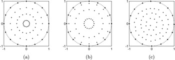
How polar-type grids create highly non-uniform resolutions in different directions near the origin. (a) Polar, equispaced in radius. (b) Polar, Chebyshev along each diameter. (c) Irregular (but avoiding clustering), as typically used in RBF contexts.

4.1.2. Test calculation: circular domain
Naturally, the earliest implementations of RBFs for PDEs were focused on showing that the approach is viable for very simple test problems. We summarize the study by Larsson and Fornberg (Reference Larsson and Fornberg2003), since this also compared RBF-Direct with Contour-Padé (the only stable choice in 2003). In order to allow easy comparisons of RBFs against FD2 (second-order FD) and PS methods, the domain was chosen as the unit circle: see Figure 4.1. All the node sets had
 $N_{B}=16$
nodes on the boundary
 $\partial {\rm\Omega}$
and
 $N_{I}=48$
nodes in the interior of
 ${\rm\Omega}$
. For FD2, the nodes were equispaced in both angle and radius, and for PS again equispaced in angle, but of Chebyshev type radially (across
 $-1\leq r\leq 1$
, with angle
 $0\leq {\it\theta}<{\it\pi}$
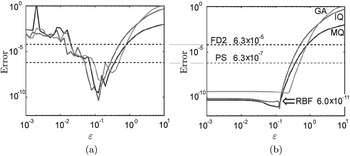
). For RBF, the nodes were somewhat irregularly scattered. Figure 4.2 shows a typical result. Here Kansa’s approach is applied to (4.1) with
 $g(\mathbf{x})$
and
 $f(\mathbf{x})$
selected in such way that the equation has as its solution
 $u(\mathbf{x})=100/(100+(x-0.2)^{2}+2y^{2})$
. Even when using RBF-Direct, the RBF approach is seen to be the most accurate option (if the optimal
 ${\it\varepsilon}$
is used). The use of a stable algorithm not only improves the accuracy further still, but also makes the choice of ‘optimal’
 ${\it\varepsilon}$
very much less critical.
It can be noted that a second-order method (such as FD2, or second-order finite elements) gains a factor of 4 in accuracy when step sizes are halved, that is, in two dimensions when four times as many nodes are used. The error is then inversely proportional to the number of nodes. In the present test case, the errors for MQ and IQ RBFs are roughly
 $10^{-6}$
times those for FD2, implying that, in order to match the RBF accuracy, FD2 would need the node count
 $N=64$
to be increased by a factor of about one million.
Max norm errors, as functions of
 ${\it\varepsilon}$
, when solving a two-dimensional Poisson test problem using three choices of RBFs, GA, IQ and MQ, using (a) RBF-Direct and (b) Contour-Padé. The dashed lines across the two subplots compare the accuracies reached by FD2, PS (both independent of
 ${\it\varepsilon}$
).

4.2. Reaction–diffusion equations on curved surfaces
Solving PDEs over curved surfaces has a substantial history, both in terms of application areas and with regard to numerical approaches. Some different methods (including RBFs) are discussed in Shankar, Wright, Fogelson and Kirby (Reference Shankar, Wright, Fogelson and Kirby2013). RBFs are particularly well-suited to the task, since they avoid the singularities that are intrinsic to any surface-bound coordinate system, exemplified for a sphere with the two poles if using spherical coordinates. Another key advantage is that spectral accuracy readily becomes available (in contrast to surface-triangularization-based finite element discretizations, for example).
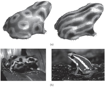
(a) Patterns produced by RBF solutions of the Brusselator reaction–diffusion equations for two different parameter settings. (b) The skin patterns on two frog species (Tabasara rain frog, and poison dart frog, respectively). Illustration provided by Cécile Piret.

The solution of PDEs over biological surfaces was pioneered by Turing (Reference Turing1952) in the context of pattern formation on animals. Both this topic, and also other processes occurring on cell surfaces and on other types of biological membranes, have since received extensive mathematical and numerical attention. The solutions presented in Piret (Reference Piret2012) use global RBFs, in combination with the orthogonal gradient method (OGr), allowing a single ‘cloud’ of nodes to be used both for defining the surface and for discretizing the PDE. Figure 4.3 illustrates an
 $N=560$
node set in the shape of a frog, and two RBF-generated solutions to the Brusselator equations over this surface. This nonlinear reaction–diffusion system closely models actual formation of skin patterns on animals (for which the time evolution gets frozen at some embryonic stage). The very high accuracy of the RBF approach is evident in Figure 4.3, as the finest resolved features have about four points per wavelength, to be compared to the theoretical limits of 2 for Fourier-PS and
 ${\it\pi}$
for Chebyshev-PS.
Fuselier and Wright (Reference Fuselier and Wright2013) describe solutions to another convection–diffusion-type PDE (the Barkley model), again over surfaces of biological objects. The global RBF approach was in this case somewhat different (a ‘projection’ approach, for which the surfaces were given in the form of level surfaces of specified three-dimensional functions).
4.3. Mantle flow in a spherical shell
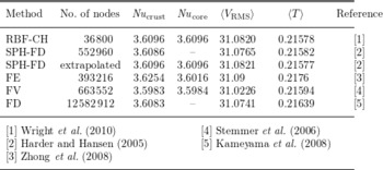
A number of increasingly large geoscience-oriented test cases were solved using global RBF-based spatial discretization between 2007 and 2011. The geometries were at first confined to the surface of a sphere (Flyer and Lehto Reference Flyer and Lehto2010, Flyer and Wright Reference Flyer and Wright2007, Flyer and Wright, Reference Flyer and Wright2009), and then followed by a three-dimensional mantle convection simulation (Wright, Flyer and Yuen Reference Wright, Flyer and Yuen2010). These works were all summarized in Flyer and Fornberg (Reference Flyer and Fornberg2011). We highlight here the mantle flow simulation, since it decisively brought RBF-based simulations from ‘just another approach that can work on toy problems’ to (i) confirming a physical prediction previously outside numerical reach, and (ii) doing so using a PC, against supercomputer calculations employing the full range of traditional methodology approaches (see Table 4.1, which abbreviates a more extensive table in Wright et al. Reference Wright, Flyer and Yuen2010).
The physical scenario is as follows: the flow is incompressible; the temperature (
 $T$
) is governed by a mixed convective–diffusive PDE; the momentum is governed by Stokes flow, an elliptic PDE; the impermeable boundaries are slip-free (Neumann boundary conditions in the angular direction), with
 $T=1$
at the core and
 $T=0$
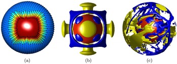
at the crust. The coupled system of three PDEs is approximated by RBF discretization on each of many concentric spherical shells, together with Chebyshev-PS discretization radially: see Figure 4.4(a). Since no analytic solutions are available, isoviscous flow at low
 $\mathit{Ra}=7\,000$
(within the steady-state regime, where
 $\mathit{Ra}$
is the Rayleigh number) has become a commonly used benchmark. The standard initial condition in this case is a combination of fourth-order spherical harmonics times linear decay in the radial direction. The summary in Table 4.1 compares results for the global variables,
 $\mathit{Nu}_{\text{crust}},\mathit{Nu}_{\text{core}},\langle V_{\text{RMS}}\rangle$
,
 $\langle T\rangle$
(
 $\mathit{Nu}$
is the Nusselt number,
 $V_{\text{RMS}}$
is the root mean square velocity, and
 $\langle \cdot \rangle$
indicates globally averaged quantities). For this test, energy conservation implies that solutions should satisfy
 $\mathit{Nu}_{\text{crust}}=\mathit{Nu}_{\text{core}}$
. The RBF-CH method, using a much lower level of discretization, achieves near-perfection in terms of accuracy compared to the previously most accurate method, the Romberg extrapolated SPH-FD method. The RBF-CH simulation was the only one that was run on standard PC hardware.
Mantle convection. (a) RBF-CH discretization. (b) Steady-state solution at
 $\mathit{Ra}=7\,000$
(colour online: yellow, upwelling; blue, downwelling; red, core). (c) Snapshot of a
 $\mathit{Ra}=10^{6}$
solution after a time corresponding to about 4.5 times the age of the Earth.

Comparison of methods in the literature for the standard
 $\mathit{Ra}=\!7\,000$
case.

Figure 4.4(c) shows a snapshot from a
 $\mathit{Ra}=10^{6}$
simulation, dominated by turbulent convection. This is a much more physically realistic case, since
 $Ra\approx 10^{7}$
for the current Earth. This RBF-CH simulation is the only spectral model in the literature to be run in spherical geometry at such a high
 $Ra$
. It showed an instability at
 $\mathit{Ra}=70\,000$
that had been theorized (Bercovici, Schubert, Glatzmaier and Zebib Reference Bercovici, Schubert, Glatzmaier and Zebib1989) but remained controversial, as it had not been seen in any previous numerical simulations. These mantle flow simulations demonstrate strikingly that global RBFs can be very competitive even on standard PCs.
5. Basic properties of RBF-FD approximations
RBF-FD combines many key strengths of RBFs with those of traditional FD approximations. The primary factor behind their development was the high computational cost of global RBFs. When using RBF-Direct, finding an interpolant or calculating a differentiation matrix (DM) each cost
 $O(N^{3})$
operations for
 $N$
nodes, with an additional
 $O(N^{2})$
operations each time a DM is applied (e.g., during time-stepping). In parallel with the successful application usage of global RBFs, as described above, efforts were under way on several fronts to dramatically reduce these costs. Of several potentially viable approaches (such as ‘fast algorithms’ based on multipole ideas, innovative preconditioners, etc.), RBF-FD is at present the leading option. The rest of this article will be devoted to this.
The RBF-FD concept was first outlined in a conference presentation by Tolstykh (Reference Tolstykh2000). Shortly afterwards it was introduced a number of times independently, for instance by Shu, Ding and Yeo (Reference Shu, Ding and Yeo2003), Wang and Liu (Reference Wang and Liu2002) and Wright (Reference Wright2003). Since this approach is still in rapid development, the present discussion will not attempt to be comprehensive but only highlight how it has already proved to be highly competitive against previous alternatives. Active application areas not discussed here include elasticity (Kee, Liu and Lu Reference Kee, Liu and Lu2008, Tolstykh and Shirobokov Reference Tolstykh and Shirobokov2003), flame propagation (Bayona and Kindelan Reference Bayona and Kindelan2013, Kindelan, Bernal, Gonzalez-Rodriguez and Moscoso Reference Kindelan, Bernal, Gonzalez-Rodriguez and Moscoso2010), and mechanics (Chinchapatnam, Djidjeli, Nair and Tan Reference Chinchapatnam, Djidjeli, Nair and Tan2009, Rodrigues, Roque and Ferreira Reference Rodrigues, Roque and Ferreira2013).
5.1. RBF-FD weights
Traditional FD approximations are grid-based and, when multidimensional, typically combine one-dimensional approximations. FD weights are determined so that the approximations become exact for polynomials of degree as high as possible. Some effective algorithms for generating FD weights are given in Fornberg (Reference Fornberg1998). The polynomial approach does not generalize well to scattered nodes in more than one dimension, with the Mairhuber–Curtis theorem being just one reason. Instead of relying on multivariate polynomials, one can enforce the exact result for all the RBFs that are centred at the nodes of the stencil of size
 $n$
. Straightforward algebra will then show that the weights
 $w_{k}$
at the stencil nodes
 $\mathbf{x}_{k},k=1,2,\ldots ,n$
can be obtained by solving the linear system
 $$\begin{eqnarray}\left[\begin{array}{@{}ccccc@{}} & & & & \\ & & & & \\ & & A & & \\ & & & & \\ & & & & \end{array}\right]\left[\begin{array}{@{}c@{}}w_{1}\\ w_{2}\\ \vdots \\ w_{n}\end{array}\right]=\left[\begin{array}{@{}c@{}}L{\it\phi}(\Vert \mathbf{x}-\mathbf{x}_{1}\Vert )|_{\mathbf{x}=\mathbf{x}_{c}}\\ L{\it\phi}(\Vert \mathbf{x}-\mathbf{x}_{2}\Vert )|_{\mathbf{x}=\mathbf{x}_{c}}\\ \vdots \\ L{\it\phi}(\Vert \mathbf{x}-\mathbf{x}_{n}\Vert )|_{\mathbf{x}=\mathbf{x}_{c}}\end{array}\right].\end{eqnarray}$$
The matrix
 $A$
is the same as the one in (2.4), and
 $\mathbf{x}_{c}$
is the location at which the stencil is approximating the
 $L$
-operator (typically chosen as a node point near the stencil centre). A common generalization of (2.3) is to add multivariate polynomials to the RBF basis, and then impose matching constraints. For instance, if one includes linear terms in a two-dimensional case, (5.1) should be replaced by
 $$\begin{eqnarray}\left[\begin{array}{@{}ccccccc@{}} & & & {\shortmid} & 1 & x_{1} & y_{1}\\ & A & & {\shortmid} & \vdots & \vdots & \vdots \\ & & & {\shortmid} & 1 & x_{n} & y_{n}\\ - & - & - & + & - & - & -\\ 1 & \cdots \, & 1 & {\shortmid}\\ x_{1} & \cdots \, & x_{n} & {\shortmid} & & 0\\ y_{1} & \cdots \, & y_{n} & {\shortmid}\end{array}\right]\left[\begin{array}{@{}c@{}}w_{1}\\ \vdots \\ w_{n}\\ -\\ w_{n+1}\\ w_{n+1}\\ w_{n+3}\end{array}\right]=\left[\begin{array}{@{}c@{}}L{\it\phi}(\Vert \mathbf{x}-\mathbf{x}_{1}\Vert )|_{\mathbf{x}=\mathbf{x}_{c}}\\ \vdots \\ L{\it\phi}(\Vert \mathbf{x}-\mathbf{x}_{n}\Vert )|_{\mathbf{x}=\mathbf{x}_{c}}\\ -\\ L\;1\;|_{\mathbf{x}=\mathbf{x}_{c}}\\ L\;x\;|_{\mathbf{x}=\mathbf{x}_{c}}\\ L\;y\;|_{\mathbf{x}=\mathbf{x}_{c}}\end{array}\right]\!,\end{eqnarray}$$
where only the weights
 $w_{1},w_{2},\ldots ,w_{n}$
should be used. For a derivation, see (Fornberg and Flyer Reference Fornberg and Flyer2015b
). The pattern in (5.2) generalizes directly to higher dimensions and different polynomial orders.
5.2. Node distributions
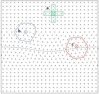
While Cartesian lattices are commonly used for FD and PS methods, hexagonal lattices (in case of two dimensions) generally allow for more cost-effective discretizations (see Section 6.2). Such lattices have been used only rarely in the past because of algebraic complexity, and difficulties with both local refinements and with generalizations to higher dimensions. When using RBFs, and especially RBF-FD, all these concerns vanish. Later in this article, Figure 6.8 will illustrate other advantages with deviating from Cartesian grids. Quasi-uniform scattered-node sets are often highly effective as well as easily generated. The Delaunay-based algorithm in Persson and Strang (Reference Persson and Strang2004) offers one convenient option. In the case of two dimensions, the algorithm described in Fornberg and Flyer (Reference Fornberg and Flyer2015a ) is particularly fast.
On Cartesian lattices, nodes are usually sequentially ordered by the lattice directions. For scattered nodes, the ordering is in principle arbitrary. However, both for achieving fast memory access (with node sets that do not fit into high-speed cache memory) and for optimal convergence rate with certain iterative linear solvers, the node ordering needs to be optimized. Reorderings based on reverse Cuthill–McGee or ‘locality sensitive hashing’ can be highly beneficial (Bollig, Flyer and Erlebacher Reference Bollig, Flyer and Erlebacher2012).
5.3. Time stabilization: hyperviscosity
For a purely convective PDE, there should not be any solution modes that feature long-term growth or decay. In the case of linear spatial operators, this can be studied via eigenvalue analysis. If the method of lines (MOL) discretization for
 $\partial u/\partial t=Lx$
takes the form
 $\text{d}\mathbf{u}/\text{d}t=D\,\mathbf{u}$
, the eigenvalues of the ‘differentiation matrix (DM)’
 $D$
should be purely imaginary. RBF-FD approximations for
 $L$
introduce a low level of ‘jitter’ on the eigenvalues, typically scattering them small distances to each side of the imaginary axis, with the physically relevant ones typically scattered the least. Whereas a small distance to the left of the axis is generally harmless (causing spurious modes to decay slowly), small scatter to the right causes exponential growth in time. What is needed is an approach that leaves the physically relevant (smooth) eigenvalues/modes intact, but ‘nudges’ spurious oscillatory ones from the right half-plane over into the left one. This can be achieved by hyper-viscosity (Fornberg and Lehto Reference Fornberg and Lehto2011), adapted from turbulence simulations. As an additional benefit, this permits the use of larger (and therefore more accurate) RBF-FD stencils. Without this enhancement, stencils in two dimensions can rarely exceed around
 $n=8-12$
nodes, whereas with the enhancement,
 $n$
-values up to around 100 were instrumental in obtaining the high accuracies reported in Flyer et al. (Reference Flyer, Lehto, Blaise, Wright and St-Cyr2012) and Fornberg and Lehto (Reference Fornberg and Lehto2011). There are at present two main hyperviscosity approaches, best-suited for global RBFs and for RBF-FD approximations, respectively.
5.3.1. The
$A^{-1}$
method

This approach applies to RBF types with the
 $A$
-matrix positive definite (e.g., GA, IQ and IMQ but not MQ or PHS). As noted in Section 3.1, the
 $A$
-matrix eigenvalues will decrease very rapidly to zero if
 ${\it\varepsilon}$
is small. The corresponding eigenvectors at the same time become increasingly oscillatory. The matrix
 $A^{-1}$
will have the same eigenvectors, but its eigenvalues are the inverses for those of
 $A$
, that is, they will start out
 $O(1)$
and then rapidly become very large (and again all positive). Hence, adding a term
 $-{\it\gamma}\,A^{-1}\mathbf{u}$
with a very small constant
 ${\it\gamma}>0$
to the right-hand side of a MOL discretization of a convective PDE
 $(\text{d}/\text{d}t)u=Lu$
will leave all the physically relevant (reasonably smooth) modes essentially intact, but will rapidly damp out all highly oscillatory (spurious noise) modes.
5.3.2. Powers of the Laplacian
The concept is again to leave smooth modes intact, but to quickly damp out rapidly oscillating high ones. Adding a small multiple of the Laplacian operator
 ${\rm\Delta}$
to the PDE’s right-hand side would damp high modes, but also interfere with low ones (which represent physical information). The analysis and test results in Flyer et al. (Reference Flyer, Lehto, Blaise, Wright and St-Cyr2012) and Fornberg and Lehto (Reference Fornberg and Lehto2011) show that using relatively high powers of
 ${\rm\Delta}$
achieves what is needed. These references discuss implementation issues, for example, guidelines for powers and multiplying factors to use, and convenient formulas for GA-type RBFs.
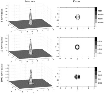
Numerical solution and magnitude of the errors for the solid-body rotation test case, using the stabilized RBF-FD approach. The displays are over the
 $({\it\varphi},{\it\theta})$
-plane, with
 ${\it\varphi}\in [-{\it\pi},{\it\pi}],{\it\theta}\in [-{\it\pi}/2,{\it\pi}/2]$
.

A standard test case for studying how well a solution is advected intact, that is, without trailing wavetrains or diffusion, is known as solid-body rotation (Williamson et al. Reference Williamson, Drake, Hack, Jakob and Swarztrauber1992). An initial condition, such as a
 $C^{1}$
cosine bell, is advected around the unit sphere at an angle
 ${\it\alpha}$
tilted relative to the polar axis. The governing equation in spherical coordinates is given by
 $$\begin{eqnarray}\displaystyle \frac{\partial h}{\partial t}+(\cos {\it\alpha}-\tan {\it\theta}\sin {\it\varphi}\sin {\it\alpha})\frac{\partial h}{\partial {\it\varphi}}+\cos {\it\varphi}\sin {\it\alpha}\frac{\partial h}{\partial {\it\theta}}=0.\end{eqnarray}$$
Using
 $N=25\,600$
MD nodes, a stencil size
 $n=74$
, GA RBFs with
 ${\it\varepsilon}=8$
, and
 ${\rm\Delta}^{8}$
-type hyperviscosity, the long-term evolution is illustrated in Figure 5.1. In spite of the very long integration time (
 $1\,000$
revolutions around the sphere), there are no visible hints of instabilities or even of loss in peak height (here less than 1%). The main errors remain right at the base of the cosine bell, where there is a jump in the second derivative.
5.4. Compact (implicit) approximations to elliptic PDEs
Since a derivative is a ‘local’ property of a function, there is something intuitively contradictory about enhancing the order of an FD approximation by invoking data located increasingly far away. When the task is to solve a PDE (rather than just to approximate an operator), compact approximations offer a different opportunity for improving the order of accuracy. For finite differences, the concept has a long history (Collatz Reference Collatz1960, Fox Reference Fox1947) with several more recent enhancements available, such as to nonlinear PDEs in two and three dimensions (Gupta Reference Gupta1991, Lele Reference Lele1992, Li, Tang and Fornberg Reference Li, Tang and Fornberg1995, Zhai, Feng and He Reference Zhai, Feng and He2013).
Before considering compact approximations in scattered-node RBF-FD cases, we illustrate the basic idea in the case of approximating
 $$\begin{eqnarray}\triangle u=\frac{\partial ^{2}u}{\partial x^{2}}+\frac{\partial ^{2}u}{\partial y^{2}}\end{eqnarray}$$
on a two-dimensional lattice, with spacing
 $h$
in each direction. The most obvious FD approximation can be written as
 $$\begin{eqnarray}\left[\begin{array}{@{}ccc@{}} & 1\\ 1 & -4 & 1\\ & 1\end{array}\right]u/h^{2}=\triangle u+O(h^{2}).\end{eqnarray}$$
Using only a
 $3\times 3$
stencil size, it is impossible to find weights that improve the accuracy above second order. Extending the stencil to five nodes in both directions permits fourth-order accuracy, but causes problems when solving the PDE
 $\triangle u=f$
.
-
(i) The centre weight becomes smaller in magnitude than the sum of magnitudes of the remaining weights, that is, diagonal dominance is lost. This damages the convergence rate of many iterative schemes, and it also opens up the possibility of system singularities.
-
(ii) Wider stencils need more boundary information than is readily available.
Taylor expansions will however reveal that, if the task is not to approximate
 $\triangle u$
but to solve
 $\triangle u=f$
, then
 $$\begin{eqnarray}\left[\begin{array}{@{}ccc@{}}1 & 4 & 1\\ 4 & -20 & 4\\ 1 & 4 & 1\end{array}\right]u/(6h^{2})=\left[\begin{array}{@{}ccc@{}} & 1\\ 1 & 8 & 1\\ & 1\end{array}\right]f/12+O(h^{4}),\end{eqnarray}$$
and for the special case of solving
 $\triangle u=0$
,
 $$\begin{eqnarray}\left[\begin{array}{@{}ccc@{}}1 & 4 & 1\\ 4 & -20 & 4\\ 1 & 4 & 1\end{array}\right]u/(6h^{2})=0+O(h^{6}).\end{eqnarray}$$
The latter approximations suffer neither of the two problems noted above, but nevertheless achieve significantly improved levels of accuracy.
Equation (5.5) can be recast as a compact approximation to
 $\triangle u$
as
 $$\begin{eqnarray}[1]\;{\rm\Delta}u=\left[\begin{array}{@{}ccc@{}}\frac{1}{4} & 1 & \frac{1}{4}\\ 1 & -5 & 1\\ \frac{1}{4} & 1 & \frac{1}{4}\end{array}\right]u/h^{2}+\left[\begin{array}{@{}ccc@{}} & -\frac{1}{8}\\ -\frac{1}{8} & & -\frac{1}{8}\\ & -\frac{1}{8}\end{array}\right]{\rm\Delta}u+O(h^{4}).\end{eqnarray}$$
RBF-FD counterparts to (5.6) for scattered nodes can readily be generated, as described in Fornberg and Flyer (Reference Fornberg and Flyer2015b ) and Wright and Fornberg (Reference Wright and Fornberg2006). The latter reference provides several test examples, showing that the advantages noted above for compact formulas carry over from lattice-based FD cases to scattered-node RBF-FD cases.
6. Three examples of solving PDEs with RBF-FD
6.1. The shallow water equations on a sphere
The equations in a three-dimensional Cartesian coordinate system for a rotating fluid are
 $$\begin{eqnarray}\displaystyle & & \displaystyle \displaystyle {\displaystyle \frac{\partial \mathbf{u}}{\partial t}}=-\,(\mathbf{u}\cdot {\rm\nabla})\mathbf{u}-f(\mathbf{x}\times \mathbf{u})-g{\rm\nabla}h,\end{eqnarray}$$
 $$\begin{eqnarray}\displaystyle & & \displaystyle \displaystyle \frac{\partial h}{\partial t}=-\,{\rm\nabla}\cdot (h\mathbf{u}),\end{eqnarray}$$
 $f$
is the Coriolis force,
 ${\rm\nabla}=\partial _{x}\hat{\mathbf{i}}+\partial _{y}\hat{\mathbf{j}}+\partial _{z}\hat{\mathbf{k}}$
,
 $\mathbf{u}=u\hat{\mathbf{i}}+v\hat{\mathbf{j}}+w\hat{\mathbf{k}}$
is the velocity vector,
 $h$
is the geopotential height and
 $\mathbf{x}=\{x,y,z\}^{T}$
represents the position vector. Working in Cartesian coordinates requires a projection operator that confines the motion to the surface of the sphere, that is,
 $$\begin{eqnarray}{\rm\nabla}\rightarrow \mathbf{P}{\rm\nabla}=[\mathbf{p}_{x}\cdot {\rm\nabla},\mathbf{p}_{y}\cdot {\rm\nabla},\mathbf{p}_{z}\cdot {\rm\nabla}],\end{eqnarray}$$
where
 $$\begin{eqnarray}\mathbf{P}{\rm\nabla}=\left[\begin{array}{@{}ccc@{}}(1-x^{2}) & -xy & -xz\\ -xy & (1-y^{2}) & -yz\\ -xz & -yz & (1-z^{2})\end{array}\right]\left[\begin{array}{@{}c@{}}\frac{\partial }{\partial x}\\ \frac{\partial }{\partial y}\\ \frac{\partial }{\partial z}\end{array}\right]=\left[\begin{array}{@{}c@{}}\mathbf{p}_{x}\cdot {\rm\nabla}\\ \boldsymbol{ p}_{y}\cdot {\rm\nabla}\\ \boldsymbol{ p}_{z}\cdot {\rm\nabla}\end{array}\right]\!.\end{eqnarray}$$
Notice that each component of the projected gradient for a given direction is a linear combination of the other three. In addition, the right-hand side of (6.1) needs to be projected, with the modified differential operators, in the corresponding
 $\hat{\mathbf{i}}$
,
 $\hat{\mathbf{j}}$
, and
 $\hat{\mathbf{k}}$
directions. For example, in the case of the
 $u$
momentum equation (corresponding to the velocity in the
 $x$
direction), this results in
 $$\begin{eqnarray}\hspace{-285.00043pt}\frac{\partial u}{\partial t}=-\mathbf{p}_{x}\end{eqnarray}$$
 $$\begin{eqnarray}\hspace{-6.00006pt}\underbrace{\cdot \left[\begin{array}{@{}c@{}}u(\mathbf{p}_{x}\cdot {\rm\nabla})u+v(\mathbf{p}_{y}\cdot {\rm\nabla})u+w(\mathbf{p}_{z}\cdot {\rm\nabla})u\\ u(\mathbf{p}_{x}\cdot {\rm\nabla})v+v(\mathbf{p}_{y}\cdot {\rm\nabla})v+w(\mathbf{p}_{z}\cdot {\rm\nabla})v\\ u(\mathbf{p}_{x}\cdot {\rm\nabla})w+v(\mathbf{p}_{y}\cdot {\rm\nabla})w+w(\mathbf{p}_{z}\cdot {\rm\nabla})w\end{array}\!+f\!\left[\begin{array}{@{}c@{}}yw-zv\\ zu-xw\\ xv-yu\end{array}\right]\!+g\!\left[\begin{array}{@{}c@{}}(\mathbf{p}_{x}\cdot {\rm\nabla})\\ (\mathbf{p}_{y}\cdot {\rm\nabla})\\ (\mathbf{p}_{z}\cdot {\rm\nabla})\end{array}\right]\!h\right]}_{\displaystyle \text{right-hand side.}}\end{eqnarray}$$
Notice that the only differential operator
 $L$
that needs to be discretized is
 $\mathbf{P}{\rm\nabla}$
, and it can be calculated as in Section 5.1. It was noticed that the addition of any polynomials beyond a constant did not affect the results. For further details see Flyer et al. (Reference Flyer, Lehto, Blaise, Wright and St-Cyr2012), which also provides a greatly simplified way to calculate the projected gradient for the sphere.
By adding a forcing term
 $h_{\text{mtn}}$
to the right-hand side of the geopotential height
 $h$
equation in (6.2), flow over a mountain can be simulated (Takacs Reference Takacs1988, Williamson et al.
Reference Williamson, Drake, Hack, Jakob and Swarztrauber1992). Two mountain profiles, one where
 $h_{\text{mtn}}$
is a
 $C^{1}$
cone and the other a
 $C^{\infty }$
mountain, are considered to illustrate the sensitivity of high-order methods to Gibbs phenomena. This is important because topographical features are rarely even
 $C^{1}$
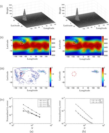
. Figure 6.1 shows the results for a 15-day run using Runge–Kutta fourth-order (RK4) time-stepping, with the reference solution given by a discontinuous Galerkin (DG) shallow water model (Blaise and St-Cyr Reference Blaise and St-Cyr2012), where each element contains
 $12\times 12$
Legendre quadrature nodes to represent the solution, which results in a total of
 $884\,736$
degrees of freedom and an average resolution around 26 km. The results are given in Figure 6.1. The key differences between the two columns of panels is that (i) even though the
 $C^{\infty }$
Gaussian mountain is slightly steeper than the
 $C^{0}$
mountain, there are no high-frequency waves emanating throughout the domain, and (ii) after
 $n=31$
, stencil size has no bearing on convergence or accuracy with the
 $C^{1}$
cone forcing. This latter fact is that with non-smooth forcing, the only way to increase accuracy is to increase resolution about the base of the mountain and not the order of the method.
(a) Cone mountain results. (i) Profile of mountain. (ii) Plotted in metres, RBF-FD solution for
 $h$
at day 15,
 $N=25\,600$
and
 $n=31$
with contour intervals at 50 m. (iii) Magnitude of the error between the RBF-FD solution and DG reference solution in metres. The contour interval is 0.5 m, with white denoting errors less than 0.1 m. (iv)
 $\ell _{2}$
-error as a function of the resolution
 $N$
for varying stencil sizes. (b) The same as (a) but for Gaussian mountain forcing. The dashed circle in all plots is the base of the mountain.

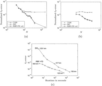
We consider three reference solutions: (i) the DG reference solution mentioned above, (ii) a spherical harmonic solution from the DWD (Deutscher Wetterdienst, German National Weather Service) that has a spectral truncation of T426, that is, it uses
 $182\,329$
spherical harmonic bases, and (iii) an RBF-FD based on
 $N=163\,824$
icosahedral-type nodes on the sphere, representing a 60 km resolution, and a stencil size of
 $n=31$
. Figure 6.2(a) shows that the
 $\ell _{2}$
-errors for the RBF-FD method, whether using the RBF-FD reference solution or a DG one, are almost identical. This same trend is also seen in Figure 6.2(b) with global RBFs. In contrast, the error from the SH reference solution is an order of magnitude larger. Given that DG, RBF-FD, and global RBFs are vastly different numerical methods, this strongly indicates that the SH spectral model is providing a less accurate solution, while DG and RBF are in line with one another.
(a,b) Convergence plots in the
 $\ell _{2}$
-norm with regard to the geopotential height fields
 $h$
for the RBF-FD (a) and global RBF (b), against the three reference solutions. Note that the RBF-FD and DG solutions agree perfectly. (c) The error as a function of computer runtime for the RBF-FD and DG methods.

The next consideration is time benchmarking of RBF-FD against DG. The present benchmarking was done on a MacBook Pro laptop with an Intel i7 2.2 GHz quad-core processor, using only a single core, and 8 GB of memory. The RBF-FD code was written in MATLAB and the DG code in C++. The RBF-FD reference solution of
 $N=163\,842$
and
 $n=31$
(i.e., 60 km resolution) was used to calculate the
 $\ell _{2}$
-error versus runtime (i.e., wall-clock time) for both methods as shown in Figure 6.2(c). The RBF-FD method was computationally faster than the DG method, from about an order and a half of magnitude for coarser resolutions to four times faster for the finest resolutions.
6.2. The compressible Navier–Stokes equations on a limited area domain
The compressible Navier–Stokes equations in a two-dimensional Cartesian coordinate system,
 $\{x,z\}$
, for stratified fluid flow (important in atmospheric processes) are as follows:
 $$\begin{eqnarray}\begin{array}{@{}ll@{}}\text{momentum} & \displaystyle \frac{\partial \mathbf{u}}{\partial t}=-\,(\mathbf{u}\cdot {\rm\nabla})\mathbf{u}-c_{p}{\it\theta}{\rm\nabla}P-g\mathbf{k}+{\it\mu}{\rm\Delta}\mathbf{u},\\ \text{energy} & \displaystyle \frac{\partial {\it\theta}}{\partial t}=-\,(\mathbf{u}\boldsymbol{\cdot }{\rm\nabla}){\it\theta}+{\it\mu}{\rm\Delta}{\it\theta},\\ \text{mass} & \displaystyle \frac{\partial P}{\partial t}=-\,(\mathbf{u}\boldsymbol{\cdot }{\rm\nabla})P-\frac{R}{c_{v}}({\rm\nabla}\cdot \mathbf{u})P,\end{array}\end{eqnarray}$$
where
 $P=(p/P_{0})^{R/c_{p}}$
is the non-dimensional Exner pressure
 $(P_{0}=1\times 10^{5}~\text{Pa})$
, and
 ${\it\theta}=T/P$
is the potential temperature. The constants
 $c_{p}=1004$
and
 $c_{v}=717$
are the specific heat at constant pressure and constant volume, respectively,
 $R=c_{p}-c_{v}=287$
, and
 ${\it\mu}$
, the dynamic viscosity. These equations are often used for testing novel numerical methods in atmospheric modelling, as will be done here.
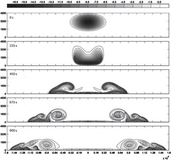
A commonly used test case is known as the Straka density current (Straka et al. Reference Straka, Wilhelmson, Wicker, Anderson and Droegemeier1993). A bubble of cold air falls to the ground and develops three smooth and distinct rotors due to shear instability, as it spreads sideways. The computational domain is
 $[-25.6,25.6]$
km in
 $x$
with periodic boundary conditions, and
 $[0,6.4]$
km in
 $z$
with no-flux and free-slip boundary conditions on the velocity and Neumann on the temperature and pressure. The dynamic viscosity is
 ${\it\mu}=75~\text{m}^{2}~\text{s}^{-1}$
. PHS RBFs,
 $r^{7}$
, together with polynomials up to third degree are used to approximate all spatial derivatives locally by the RBF-FD approach with a stencil size of
 $n=37$
. The remaining system of first-order ODEs is time-stepped with RK4. Figure 6.3 shows the behaviour of the numerical solution in time from
 $t=0~\text{s}$
until the final time
 $t=900~\text{s}$
.
The time evolution of the potential temperature
 ${\it\theta}$
using a hexagonal node layout at 100 m resolution.

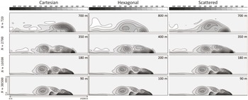
The RBF-FD approach makes it particularly easy to test how different node distributions (all with the same total number of nodes) influence the extent to which the physics is captured. In Figure 6.4, three different node layouts are examined: Cartesian, hexagonal, and quasi-uniformly scattered. Convergence under refinement leads in all cases to the same solution, as seen in the highest-resolution displays (bottom row). However, in numerical weather prediction, the ability to work at such fine resolutions as 100 m is a luxury rather than a reality. The fact that observational data that initialize models are observed on the order of kilometres, makes the degree to which the physics is captured at coarser resolutions more important. Three key features to be noticed are: (i) formation of the rotors, (ii) how much cold air they have entrenched (larger negative values of
 ${\it\theta}$
, black) and (iii) where the front location is. In the coarsest case shown, using only 720 nodes in the domain (about 700 m resolution), the hexagonal and scattered-node calculations give more clear evidence of the first rotor being formed. At the next-higher resolution (
 $2\,700$
nodes in the entire domain, about 3
 $50~\text{m}$
resolution), they provide a better picture of the formation of subsequent rotors, as well as more accurate entrenchment of cold air (black) near the front, looking more similar to the high-resolution 90 m case. Cartesian nodes furthermore give solutions more prone to Gibbs phenomenon oscillations (overshoots in white of
 $2.4~\text{K}$
as opposed to
 $1~\text{K}$
).
The calculations for Figure 6.4 all used RBF-FD stencils of size
 $n=37$
, generated from
 ${\it\phi}(r)=r^{7}$
, supported with polynomials up through degree 3. The differences between the columns of subplots reflect only the intrinsic resolution capabilities of the different node layouts. The traditional Cartesian choice is the least effective one. If using a fixed node separation, a hexagonal layout can ‘pack’ more nodes into a fixed region than a Cartesian one. Conversely, in the present case with fixed node numbers, their separation becomes somewhat larger. Even so, at every resolution level, the hexagonal choice gives better accuracy than the Cartesian one. The big advantage of generalizing further, from hexagonal to quasi-uniformly scattered nodes, is that it then becomes trivial to implement spatially variable node densities, that is, to do local refinement in select critical areas. It is very important to note that this major increase in geometric flexibility (from hexagonal to quasi-uniformly scattered) hardly has any negative effect at all on the accuracy that is achieved, nor on the algorithmic complexity of the code.
The potential temperature
 ${\it\theta}$
for the Straka density current test case at the final time
 $t=900~\text{s}$
, shown as a function of the total number of nodes when using the RBF-FD method on different node sets. For plot clarity, only half of the solution is displayed.

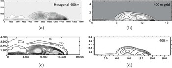
To place Figure 6.4 in context with the results of other numerical methods, a comparison is done with DG, spectral element (SE), finite volume (FV), and upwinding schemes in Figure 6.5. As can be seen, when no filtering is used in the RBF-FD method, there is a trade-off between capturing features at low resolutions and preserving monotonicity. Only the FV and upwind schemes do not exhibit Gibbs’ oscillations and have solutions with monotonic properties. However, the price to be paid is that the solution is smoothed out both with regard to rotor formation and the amount of cold air that has been entrenched. The DG and SE solutions have more structure, but the beginning formation of the second rotor is still not seen as well as in the RBF-FD model.
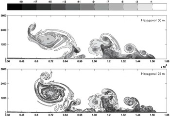
Without any explicit viscosity, the solution enters the turbulent regime with the dynamics now modelled by the Euler equations. In such regimes, there is no convergence to any solution as energy cascades to smaller and smaller scales, eventually entering the subgrid-scale domain. Nevertheless, it is interesting to observe whether the model remains stable in this regime. Figure 6.6 shows the solution at
 $50~\text{m}$
and
 $25~\text{m}$
resolutions on a hexagonal layout (optimal in two dimensions and easily implemented with RBFs). The fact that now there is no explicit viscosity, that is,
 ${\it\mu}=0$
in (6.4), does not affect the time stability, and the time step did not have to be altered between the two cases. Stability is governed solely by the fact that the time step could not exceed the speed of sound in air.
Comparison at
 $400~\text{m}$
between four different numerical methods: (a) RBF-FD (Barnett, Flyer and Wicker Reference Barnett, Flyer and Wicker2015), (b) fifth-order upwind advection, (c) discontinuous Galerkin and spectral element, eighth-order, (d) finite volume solver. Contour intervals: (a)
 $1~\text{K}$
, (b)
 $1~\text{K}$
, (c)
 $0.25~\text{K}$
, (d)
 $1~\text{K}$
.
Figures 6.5(b), 6.5(c) and 6.5(d) are reproduced with the kind permission of Elsevier. All three plots are from the Journal of Computational Physics: (b) is from Figure 4 of Skamarock and Klemp (Reference Skamarock and Klemp2008, p. 3475); (c) is from Figure 7 of Giraldo and Restelli (Reference Giraldo and Restelli2008, p. 3869); (d) is from Figure 5 of Norman, Nair and Semazzi (Reference Norman, Nair and Semazzi2011, p. 1578).

The potential temperature
 ${\it\theta}$
for the Straka density current test case with the dynamic viscosity
 ${\it\mu}=0$
on a hexagonal node layout of
 $50~\text{m}$
and
 $25~\text{m}$
.

6.3. Forward seismic modelling
6.3.1. Background
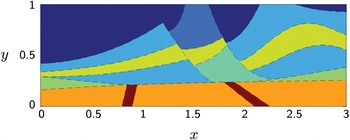
Seismic exploration is the primary tool used for finding and then mapping out hydrocarbon deposits. In forward modelling, subsurface structures are assumed to be known, and the task is to simulate elastic wave propagation through the medium. Inversion programs then update subsurface assumptions to reconcile the model response with actual measurements. There are typically hundreds of irregularly curved interfaces present, often interrupted by fracture lines with associated translations between the strata on the two sides. During the history of the earth, the vast majority of all hydrocarbons (such as natural gas and oil), being lighter than water, have migrated up to the surface and then biodegraded. What is left are mostly small pockets where hard layers have somehow formed traps for this upward migration, due to their curvature or the presence of corners resulting from fractures. With drilling being far more expensive (and environmentally damaging) than seismic exploration, the latter is constantly pushed to its limits, leading to some of the largest computational tasks in any field.
Figure 6.7 shows a extremely simplified model for the Marmousi test case, itself a highly simplified two-dimensional vertical slice off the coast of Madagascar (as shown in Figure 2 of Martin, Wiley and Marfurt Reference Martin, Wiley and Marfurt2006). The governing elastic wave equations in two dimensions are
 $$\begin{eqnarray}\displaystyle \begin{array}{@{}rcl@{}}\displaystyle {\it\rho}u_{t} & = & \displaystyle f_{x}+g_{y},\\ \displaystyle {\it\rho}v_{t} & = & \displaystyle g_{_{x}}+h_{y},\\ \displaystyle f_{t} & = & \displaystyle ({\it\lambda}+2{\it\mu})\hspace{2.22198pt}u_{x}+{\it\lambda}v_{y},\\ \displaystyle g_{t} & = & \displaystyle {\it\mu}\hspace{2.22198pt}(u_{x}+v_{y}),\\ \displaystyle h_{t} & = & \displaystyle ({\it\lambda}+2{\it\mu})\hspace{2.22198pt}v_{y}+{\it\lambda}u_{x}.\end{array} & & \displaystyle\end{eqnarray}$$
The dependent variables are
 $u,v$
(horizontal and vertical velocities) and
 $f,g,h$
(components of the symmetric stress tensor), and the material is specified by
 ${\it\rho}$
(density) and
 ${\it\lambda},{\it\mu}$
(Lamé parameters for compression and shear). Away from interfaces, these equations support two types of waves: P-waves (pressure or primary) with speed
 $c_{p}=\sqrt{({\it\lambda}+2{\it\mu})/{\it\rho}}$
, and S-waves (shear or secondary) with speed
 $c_{s}=\sqrt{{\it\lambda}/{\it\rho}}$
. Each incoming wave to an interface generally results in four main outgoing waves: reflected and transmitted P-waves and S-waves (and possibly also waves following interfaces). With typically hundreds of interfaces, wave patterns become extremely complicated. Simulated return signals at the surface need to accurately represent wave propagation for long distances through regions with smoothly varying material properties, as well as reflection-transmissions (with respect to amplitudes, phase angles, and directions).
Subsurface acoustic velocities in a ‘micro-Marmousi’ test case.

In the smoothly varying regions, the dominant error source is numerical dispersion. The only practical remedy for this is to use high-order approximations (Fornberg Reference Fornberg1987). The industry standard moved from second to fourth order in the 1980s, and FD approximations of extremely high (around
 $20$
th) order are now in common use. It has proved much more difficult to achieve accurate interface treatments (Lombard and Piraux Reference Lombard and Piraux2004, Lombard, Piraux, Gelis and Virieux Reference Lombard, Piraux, Gelis and Virieux2008, Symes and Vdovina Reference Symes and Vdovina2009). While closed-form expressions are available in simplified cases (such as straight interfaces between constant media), incorporating these in full production codes has so far not been cost-effective. Surprisingly, it has become standard procedure in the industry to omit special treatment (beyond the mild smoothing of interfaces), accepting, typically, first-order convergence for reflected waves. The present RBF-FD/AC method (with AC standing for analytic correction) achieves third-order accuracy both in smooth regions and across smoothly curved interfaces, making it very competitive.
6.3.2. RBF-FD/AC approach
Figure 6.8 illustrates a typical node layout and the different stencil types used in an even more simplified test case, with just one curved interface in two dimensions. The nodes are distributed to straddle the interface but then smoothly transition to become lattice-based a short distance away from it. Three stencil types are used: (a) regular FD when the whole stencil is lattice-based, (b) standard RBF-FD where some nodes are irregularly placed, while away from the interface, and (c) RBF-FD/AC when an interface intersects a stencil.
The three stencil types (a), (b), (c) used in a hybrid approach combining FD with RBF-FD/AC.

The naïve supporting monomials up through degree 4 compared to the interface-specific ones in the special case of
 $c_{L}=1,c_{R}=2,{\it\rho}_{L}={\it\rho}_{R}=1.$

Although the RBF-FD/AC discretization has been successfully tested in one, two and three dimensions, we limit ourselves here to describing it in one dimension (for a two-dimensional description: see Martin, Fornberg and St-Cyr Reference Martin, Fornberg and St-Cyr2015). The governing equation reduces in one dimension to
 $$\begin{eqnarray}\frac{\partial }{\partial t}\left[\begin{array}{@{}c@{}}u\\ f\end{array}\right]=\left[\begin{array}{@{}cc@{}}0 & \frac{1}{{\it\rho}}{\textstyle \frac{\partial }{\partial x}}\\ {\it\rho}c^{2}{\textstyle \frac{\partial }{\partial x}} & 0\end{array}\right]\left[\begin{array}{@{}c@{}}u\\ f\end{array}\right]\!.\end{eqnarray}$$
While
 ${\it\rho}$
and
 $c$
typically both jump at an interface, continuity of motion and traction requires
 $u$
and
 $f$
to be continuous (in the two-dimensional case, there will similarly be four continuity relations linking the five variables in (6.5)). Denoting left and right sides of the interface by subscripts
 $L$
and
 $R$
respectively, it will then hold that
 $$\begin{eqnarray}\left[\begin{array}{@{}c@{}}u_{L}\\ f_{L}\end{array}\right]-\left[\begin{array}{@{}c@{}}u_{R}\\ f_{R}\end{array}\right]=\left[\begin{array}{@{}c@{}}0\\ 0\end{array}\right]\!,\end{eqnarray}$$
which implies
 $$\begin{eqnarray}\frac{\partial ^{k}}{\partial t^{k}}\left\{\left[\begin{array}{@{}c@{}}u_{L}\\ f_{L}\end{array}\right]-\left[\begin{array}{@{}c@{}}u_{R}\\ f_{R}\end{array}\right]\right\}=\left[\begin{array}{@{}c@{}}0\\ 0\end{array}\right]\!,\quad k=0,1,2,\ldots .\end{eqnarray}$$
With use of (6.6), these time identities will translate to relations between spatial derivatives for
 $u$
and
 $f$
on the two sides. The idea is to embed these relations in the supplementing polynomials for the RBF-FD approximation (but not in the RBFs themselves: see Yu and Chen Reference Yu and Chen2011, where a similar approach was considered in the context of Maxwell’s equations). Figure 6.9 illustrates how one thus arrives at ‘interface-aware’ supplementary polynomials (with their changes across the interface dependent on the material properties on the two sides).
6.3.3. Two-dimensional test case
In the geometry shown in Figure 6.7, Figure 6.10(a) (overleaf) shows the vertical velocity
 $v$
associated with an underground explosive source, and Figure 6.10(b) a very accurate calculation of the solution at a certain later time. Figures 6.10(c) and 6.10(d) display the error at this same later time for RBF-FD/AC solutions when using
 $N=38\,400$
and
 $N=153\,600$
nodes, respectively (using IMQ-type RBFs: stencils of type (b), as shown in Figure 6.8,
 $n=19$
, polynomials degree 3; stencils of type (c),
 $n=38$
, polynomials degree 2). Since the colour bars for these latter two cases (Figures 6.10(c) and 6.10(d)) are identical, one can readily note that halving the typical node separation
 $h$
has reduced the error by more than a factor of ten. For a scheme that is third-order accurate everywhere, the expected error reduction would have been a factor of eight.
Test calculation for the ‘micro-Marmousi’ example using the RBF-FD/AC approach, showing better than a factor of 10 reduction in error when the number of nodes is doubled. (a) Initial condition for
 $v$
at
 $t=0$
, (b) solution for
 $v$
at
 $t=0.3$
, (c) RBF-FD/AC error,
 $N=38\,400$
nodes, (d) RBF-FD/AC error,
 $N=153\,600$
nodes.

7. Conclusions
Ever since RBFs were first introduced for multivariate interpolation, their range of applications has grown tremendously. In some sense, computational experiences with RBFs for PDEs are now well ahead of the more strict analysis of these methods. With so many free parameters associated with irregularly scattered nodes, strict numerical analysis obviously becomes far more difficult than for lattice-based methods, such as FD or PS. This lack of rigorous theory, for example with regard to stability during time-stepping, might have somewhat delayed the broad adoption of RBF-based methods for large applications. However, the number of successful large-scale benchmark comparisons against alternative PDE approaches is now steadily increasing. The present authors hope that this will stimulate new advances on all fronts of the topic of RBFs for PDEs: theoretical, computational, as well as still further extending the range of application areas.
Acknowledgements
This research was supported by NSF grants DMS-0914647, DMS-0934317, OCI-0904599 and by Shell International Exploration and Production, Inc.