

In the previous issue, we looked at Cohen's kappa (κ), a statistic that is very often used to measure agreement between raters for both nominal and ordinal ratings. An important consideration in any study examining inter-rater agreement is whether the study's sample size is sufficiently large so the researchers can be highly confident that they will be able to declare that the difference between the kappa observed in the study (κ 1) and some other (usually) lower value (κ 0) is statistically significant (provided, of course, such a difference exists in the population). This is a question of sample size estimation and statistical power.
As we will see below, the required sample sizes are not trivial, and perhaps the biggest hurdle in psychiatric and psychological research is obtaining sufficient ratings from two raters. When the ratings involve, for example, clinical assessments for the presence of a disorder or for the presence of a symptom from a rating scale, finding two raters for each patient can be a real difficulty. This task is often made harder if the patient has to be observed at the same time by the two raters, and it is not possible to use video recordings. Unfortunately, as a result, it is likely that many studies are quite underpowered, that is, have used far too few ratings.
Researchers usually perform significance testing using a null hypothesis where the value of the statistic is zero: the difference between two means is zero; the correlation between two variables is zero and so on. Sometimes this is not very informative, and comparing κ to zero is a good example where a non-zero null is preferable. Showing that you have better agreement than random agreement is rarely of much interest, as typically one wants to show a high level of agreement and, especially, that it is better than the moderate level of agreement that one would routinely expect, but usually would find unacceptable or poor, and for that reason significance tests need to show that κ 1> κ 0, where κ 0 is greater than 0. A reasonable choice for κ 0 is likely to vary across domains as these differ in the precision with which diagnoses or ratings of features are made, or are required to be made. In psychiatry, a range of 0.4–0.6 would seem reasonable. If we are making binary ratings and around half of the patients are positive, then this range corresponds to raw agreement of some 70–80%. Alas, of course, sample sizes are much larger for κ 0 = 0.4 than for κ 0 = 0.
Power estimation for kappa is not as firmly developed as it is for some other commonly used statistics and the estimates are more approximate. One reason for this is that the power depends not only on κ 1 and κ 0, but also on the proportion of the subjects that are put into each category by each rater, and these proportions (called marginal frequencies) will not be the same for both raters. In practice, we need to distinguish between ratings where there are only two categories (2 × 2 tables) and those where there are more (e.g. 4 × 4), although beyond 4 or 5, other statistics offer better options for assessing agreement. For the 2 × 2 table, Flack et al. Reference Flack, Afifi and Lachenbruch(1) and Donner and Eliasziw Reference Donner and Eliasziw(2) provided different methods, although both of them assume that the marginal frequencies are the same for both raters. (Cantor Reference Cantor(3) extended the work done by Flack et al. Reference Flack, Afifi and Lachenbruch(1) to include the situation where the marginal frequencies are not the same.) Using the calculations in Reference Donner and Eliasziw(2) gives larger estimates of sample size. For tables 3 × 3 and larger, the methods described in Reference Flack, Afifi and Lachenbruch(1) need to be used.
From the point of view of the researcher, the complexity arises because not only does one need to decide on what kappa one anticipates finding, but also on the marginal frequencies, and even if one assumes the same for both raters, there are clearly many possibilities.
For the 2 × 2 graphs below, we have used the calculations given in Reference Donner and Eliasziw(2) for the calculations as this approach's accuracy is better established than those in Reference Flack, Afifi and Lachenbruch(1) for the other graphs. In keeping with earlier comments, we have set the null hypothesis value to κ 0 = 0.4. As most researchers want to test the directional hypothesis that κ 1> κ 0, we have used the one-tailed test in Reference Flack, Afifi and Lachenbruch(1,Reference Cantor3), rather than the two-tailed test used for the non-directional hypothesis κ 1≠κ 0 in Reference Donner and Eliasziw(2); all methods of course can test either hypothesis. Finally, the type I error rate is set to 0.05.
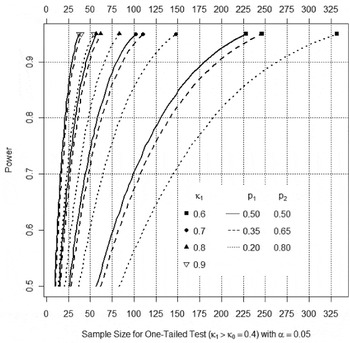
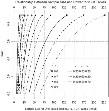
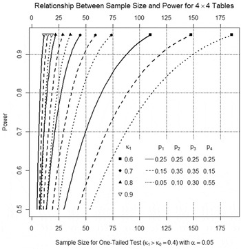
Figures 1–3 show the relationship between sample size and power, so that for the conditions examined, we can either read power achieved by a given sample size or the sample required for a given power. To make the graphs more readable, power is limited to 50% or greater.
Relationship between power and sample size when testing κ 1 > 0.4 for four values of κ 1 and three configurations of marginal frequencies (p 1 and p 2) in a 2 × 2 table.

Relationship between power and sample size when testing κ 1 > 0.4 for four values of κ 1 and three configurations of marginal frequencies (p 1, p 2 and p 3) in a 3 × 3 table.

Relationship between power and sample size when testing κ 1 > 0.4 for four values of κ 1 and three configurations of marginal frequencies (p 1, p 2, p 3 and p 4) in a 4 × 4 table.

Each figure shows curves for four values of κ 1 (the value of kappa the researcher expects): 0.6, 0.7, 0.8 and 0.9. In turn, each value of kappa is examined under three different configurations of the marginal frequencies. For all tables, one configuration consists of equal frequencies for all categories and at least one configuration where the frequencies increase. For the 3 × 3 and 4 × 4 tables, there is also a configuration where the bulk of the ratings occur in the middle. In all cases, the actual ordering of the frequencies is irrelevant for these calculations (i.e., there is no difference between nominal and ordinal ratings).
As can be seen from the figures, there are many cases where the sample size is onerous particularly given the problems noted above. Note how power decreases (sample size increases) as the marginal frequencies become less equal – clearly, a realistic assessment of how often each category on an item or scale is going to be used (broadly speaking, knowing how severe our patients are) is important in planning a study. Finally, keep in mind that if one wants to use two-tailed tests, the sizes of these samples can increase substantially, often in the order of 25–40%.