




1. Introduction
The acoustic duration of segments is known to be influenced by a variety of factors, including speech rate, frequency, prosodic structure and phonological features (Klatt Reference Klatt1973, Gahl Reference Gahl2008, Fletcher Reference Fletcher, Hardcastle, Laver and Gibbon2010). The duration of segments in any given morphFootnote 1 can then be further influenced by morphological factors. A famous example is the case of segmentally homophonous morphs, which have been demonstrated to show subtle differences in acoustic duration.
One of the earliest reports of acoustic differences between homophones was the study by Walsh & Parker (Reference Walsh and Parker1983), which compared the duration of plural /s/ and non-morphemic /s/ in three English homophone pairs (e.g. lapse vs. lap-s). Walsh & Parker (Reference Walsh and Parker1983) found plural /s/ to be ca. 10ms longer than non-morphemic /s/. Lavoie (Reference Lavoie2002) observed differences in compressibility and range of realizations between the preposition for and the numeral four in that the preposition exhibits more extreme reduction possibilities than the numeral. Gahl (Reference Gahl2008) reported a shorter duration for time compared to the homophonous noun thyme, which can be attributed to stark differences in lemma frequency. Drager (Reference Drager2011) noted systematic phonetic variation between three types of like in English (quotative, particle, lexical verb), and also differences between speakers and various social groups in the realization of these three lexemes. Plag et al. (Reference Plag, Homann and Kunter2017) investigated the duration of various /s/ and /z/ morphs (corresponding to orthographic <s>) in English based on data from the Switchboard corpus (Godfrey & Edward Reference Godfrey and Edward1997). The study compared a total of seven homophonous <s>: the third-person singular suffix, the plural suffix, the genitive singular enclitic, the genitive plural enclitic, the cliticized forms of has and is, and non-morphemic <s>. The authors observed that non-morphemic and plural <s> were substantially longer than the other <s> suffixes, while the cliticized variants of has and is had the shortest durations. In a related study, Seyfarth et al. (Reference Seyfarth, Garellek, Gillingham, Farrell and Malouf2017) found that morphologically complex English forms like free-s tend to have longer durations than homophonous freestanding forms like freeze, which the authors attribute to a paradigm uniformity effect matching the timing of articulatory gestures in free-s to that of the base form free.
For humans to communicate efficiently, there is an obvious tension between the benefit of the phonetic disambiguation of homophones and the increased effort of controlling the duration of individual morphs at a sub-phonemic level. It is an open question whether consistent acoustic differences between homophones exist across a large and diverse sample of languages while controlling for known effects such as frequency, pre-boundary lengthening, etc. The hypothesis I want to put forward here is that the case of the English <s> homophones examined by Plag et al. (Reference Plag, Homann and Kunter2017) is extraordinary for a number of reasons, and that homophones that share certain properties with English <s> are more prone to showing acoustic differences compared to other homophones. In my view, there are three particular grounds on which English <s> homophones need to be considered exceptional. First, the <s> homophone setFootnote 2 in English is extremely crowded. Plag et al. (Reference Plag, Homann and Kunter2017) discuss six different morphemes that all share the same phonological exponent or set of exponents, plus non-morphemic <s>. This extreme density is the result of phonetic convergence and morphological simplification over time, and cross-linguistically, it is rather uncommon for one morph to compete with five or more homophonous morphs. A sensible question to ask is whether acoustic differences between homophones are limited to, or more likely to occur in, highly crowded homophone sets, as compared to smaller groups with two or three homophones.
Second, the alveolar fricative /s/ is one of the most common and perceptually salient consonants in the world’s languages (Maddieson & Disner Reference Maddieson and Disner1984). What sets /s/ apart from most other fricatives is its high inter-speaker variability combined with a low within-speaker variability (Gordon et al. Reference Gordon, Barthmaier and Sands2002, Smorenburg & Heeren Reference Smorenburg and Heeren2020, Chodroff & Wilson Reference Chodroff and Wilson2022). /s/ requires fine motor control and tactile feedback and shows considerable coarticulatory resistance (Recasens Reference Recasens2018). Sociophonetic research suggests fine phonetic detail in /s/ production and perception can be employed to mark social status (Stuart-Smith Reference Stuart-Smith, Cole and Hualde2007), gender (Weirich & Simpson Reference Weirich and Simpson2015) and sexual orientation (Linville Reference Linville1998, Munson et al. Reference Munson, McDonald, DeBoe and White2006, Mack & Munson Reference Mack and Munson2012, Nylén et al. Reference Nylén, Holmberg and Södersten2024). Due to the sociophonetic versatility of /s/, it is plausible that morphs containing /s/ (or its voiced counterpart /z/) may also fulfill additional functions related to the acoustic disambiguation of homophones.
A third feature shared by all <s> morphs investigated by Plag et al. (Reference Plag, Homann and Kunter2017) is their templatic homogeneity – that is, their morphological status as suffixes and enclitics occurring in the post-stem domain (or at the right edge of stems in the case of mono-morphemic <s>). This homogeneity exacerbates the confusability for the various <s> morphs, which raises the question whether homophonous morphs occupying different templatic positions (such as a prefix and a suffix) will show similar temporal differences. In a mixed group of homophonous morphs where one morph is a root and the other is an affix, one would also expect the root to be longer based on the fact that roots are phonologically stronger than affixes (Beckmann Reference Beckmann1998). The present paper therefore seeks to answer two fundamental questions: First, what role does morphology play in accounting for durational differences between segmentally homophonous morphs across languages? And second, do homophonous morphs that are highly susceptible to acoustic disambiguation share certain properties with each other, and with the English <s> homophones?
The remainder of the paper is structured as follows. Section 2 provides an overview of previous literature on homophony and phonetic traces of morphology. Section 3 introduces the multilingual corpus used in this study and outlines the methods applied to assess the role of lexical identity in explaining temporal differences between homophonous morphs. Section 4 presents the results of the study and offers a discussion of potential factors affecting the likelihood by which homophone sets become susceptible to acoustic disambiguation. Section 5 discusses the results in light of grammatical theories and highlights potential avenues for follow-up research. Section 6 summarizes the main findings of the study.
2. Literature review
A standard definition of homophony requires that two phonologically identical forms have two unrelated meanings (1). Sometimes, the term homophony is used more loosely and extends to cases of polysemy, metonymy and syncretisms. All of these phenomena have in common that two phonologically identical forms differ in at least one semantic or grammatical detail. However, delineating these differences is not always straightforward, and the boundaries between these types of relations may depend on the particular framework or research question.
(1)
Homophony
Two linguistic units have the same phonological form but two unrelated meanings.
Vicente & Falkum (Reference Vicente and Falkum2017) emphasize the relatedness criterion to distinguish homophony from polysemy, and critically evaluate the boundaries of reducing two meanings to one core meaning. Valera (Reference Valera2020) deals with processes resulting in the emergence of homophones, including sound change (phonological convergence), semantic change (semantic divergence), and borrowing. In typology, a key concept related to homophony is colexification, which refers to the phenomenon whereby a single lexical item expresses multiple distinct meanings across different contexts (Rzymski et al. Reference Rzymski, Tresoldi, Greenhill, Wu, Schweikhard, Koptjevskaja-Tamm, Gast, Bodt, Hantgan, Kaiping, Chang, Lai, Morozova, Arjava, Hübler, Koile, Pepper, Proos, Van Epps, Blanco, Hundt, Monakhov, Pianykh, Ramesh, Gray, Forkel and List2020). Colexification is common across languages, and languages show certain preferences for expressing closely related meanings with the same linguistic form. Cross-linguistic tendencies in the co-expression of grammatical categories have similarly been analyzed in terms of semantic maps (Haspelmath Reference Haspelmath and Tomasello2003, Cysouw Reference Cysouw, Miestamo and Wälchli2007). In the context of language documentation data, drawing a clear line between homophony and other semantic relations is particularly challenging when the amount and detail of available material is limited (Rice Reference Rice, Lieber and Štekauer2014). Moreover, the bulk of existing research on acoustic disambiguation focuses on homophones such as lexical homophones or homophonous grammatical markers, with few exceptions (Schlechtweg et al. Reference Schlechtweg, Heinrichs, Linnenkohl and Schlechtweg2020). For that reason, the present study will take a conservative stance and limit itself to homophonous elements that can with some degree of certainty be considered semantically unrelated.Footnote 3
Even though homophony is a widespread phenomenon in human language, homophone sets are challenging for efficient communication because they introduce ambiguity that may lead to confusion. It is thus not surprising that languages show a certain dispreference towards homophones, which can manifest itself in various ways. Apart from subtle acoustic differences, homophony avoidance may operate on many levels, from affix selection in inflectional paradigms and conditions governing suppletive allomorphy to incomplete neutralization and inhibited sound change in phonology. Munteanu (Reference Munteanu2021) noted that Russian stressed case allomorphs -ú ‘-prep.sg’ and -á ‘-nom.pl’ tend to be selected by stems where a homophonous form with an unstressed case suffix occurs elsewhere in the inflectional paradigm. Goudswaard (Reference Goudswaard2004) argued that homophony avoidance drives the choice between two suppletive infixes in Ida’an-Begak past tense paradigms. Goudswaard alleged that verbs starting with a consonant followed by /i/ select the -әn- past tense infix over the expected -i- infix because the latter would create an output that is homophonous with the base form. Within the framework of Optimality Theory, the empirical domain of homophony avoidance has seen proposals revolving around the RealizeMorpheme constraint (Kurisu Reference Kurisu2001) or transderivational anti-faithfulness constraints (Benua Reference Benua2000). Tomaschek & Berg (Reference Tomaschek and Berg2023) reported that the contrast between German [ɐ] and [a] in unstressed syllables, which is generally assumed to be neutralized for Standard German, is in fact maintained in quasi-homophonous pairs such as Opa ‘grandpa’ and Oper ‘opera’ (but see Rathcke & Mooshammer Reference Rathcke and Mooshammer2022 for a similar study finding conflicting evidence). Blevins & Wedel (Reference Blevins and Wedel2009) critically examined cases of inhibition of sound change that would have resulted in the creation of homophony.
The acoustic duration of linguistic units is subject to various influences.Footnote 4 The frequency of words, and of linguistic units more generally, is known to affect their acoustic shape, with high-frequency items often being associated with phonetic reduction or phonological erosion (Zipf Reference Zipf1935, Bybee Reference Bybee2002, Pluymaekers et al. Reference Pluymaekers, Ernestus and Baayen2006, Strunk et al. Reference Strunk, Seifart, Danielsen, Hartmann, Pakendorf, Wichmann, Witzlack-Makarevich and Bickel2020, Linders & Louwerse Reference Linders and Louwerse2023). Frequency has been explicitly identified as a factor driving durational differences between lexical homophones (Gahl Reference Gahl2008). The size of words (in terms of phonological or morphological units) affects duration through two closely related effects known as polysyllabic shortening (Lehiste Reference Lehiste1972) and Menzerath’s Law (Stave et al. Reference Stave, Paschen, Delafontaine and Seifart2021), which both state that there is an inverse relation between the size of units and the duration of the respective sub-units. The segmental context within a word plays a key role for the duration of phones due to coarticulatory effects, most notably the fact that vowels tend to be longer before voiced than before voiceless consonants (Chen Reference Chen1970, Beckman & Edwards Reference Beckman and Edwards1980). The segmental context can be extended to word boundaries, which may also affect the duration of boundary-adjacent segments. Lengthening of word-initial consonants has been reported to be pervasive across languages (Blum et al. Reference Blum, Paschen, Forkel, Fuchs and Seifart2024), while lengthening of word-final vowels appears to be a language-specific process (White et al. Reference White, Benavides-Varela and Mády2020).
As far as larger prosodic domains are concerned, the position of words also plays a key role in determining acoustic duration. Most prominently, Final Lengthening increases segmental duration in up to two syllables before a major prosodic boundary (Turk & Shattuck-Hufnagel Reference Turk and Shattuck-Hufnagel2007, Fletcher Reference Fletcher, Hardcastle, Laver and Gibbon2010). Final Lengthening is attested in a wide variety of languages, and the lack of known counter-examples suggests it may be a (quasi-)universal process in human speech (Paschen et al. Reference Paschen, Fuchs and Seifart2022). In addition, local speech rate is a natural source of variation in segmental duration: in stretches of speech when a speaker talks fast, the duration of phones, and by extension the duration of morphs, is shorter than when a speaker talks more slowly. Speech rate varies extensively across languages and individuals, and also between utterances from the same speaker (Coupé et al. Reference Coupé, Oh, Dediu and Pellegrino2019, Strunk et al. Reference Strunk, Seifart, Danielsen, Hartmann, Pakendorf, Wichmann, Witzlack-Makarevich and Bickel2020, Tilsen & Tiede Reference Tilsen and Tiede2023). In general, variation across and within speakers is a strong influence on acoustic duration, and this variable also interacts with some of the other variables (for example, see Esposito Reference Esposito2020 on gender-related differences in the degree of Final Lengthening).
In addition to these factors, morphological structure has been observed to manifest itself acoustically in various ways. Zuraw et al. (Reference Zuraw, Lin, Yang and Peperkamp2021) noted that the duration of onset voice onset time (VOT) depends on morphological segmentability in English prefixed and pseudo-prefixed words such as dis-claimer vs. disco, with long VOT indicating the presence of a strong boundary and transparent semantics. In a study on German syncretic singular and plural nouns, Schlechtweg et al. (Reference Schlechtweg, Heinrichs, Linnenkohl and Schlechtweg2020) found plural forms to be longer than singular forms. Schmitz & Baer-Henney (Reference Schmitz and Baer-Henney2024) found subtle differences in duration between non-morphemic and suffixal word-final /s/ in German pseudowords. Regarding the perception of morpho-phonetics, Kemps et al. (Reference Kemps, Mirjam Ernestus and Baayen2005) reported Dutch speakers to be sensitive to prosodic differences between singular nouns and their homophonous stem forms in plural nouns. Similarly, Schmitz (Reference Schmitz2022) showed that speakers of English are sensitive to durational mismatches in word-final /s/.
However, internal morphological structure and lexical identity are not always detectable in the acoustic signal. In a reading experiment with speakers of British English, Schlechtweg & Corbett (Reference Schlechtweg and Corbett2021) did not find significant differences in the duration of plural -s in regular plural nouns compared to pluralia tantum nouns. Wu (Reference Wu2017) investigated various factors influencing word duration in Chinese and reports no significant effect of the internal structure of compounds on duration. Morrison (Reference Morrison2021), in a production experiment measuring nasal airflow, found no support for traces of underlying nasal features in Scottish Gaelic mutated consonants. For most of the world’s 7000 languages, no data on the interplay between morphology and phonetics exist to date. It is thus still an open question just how common phonetic reflections of morphological structure truly are across languages, and whether acoustic disambiguation of homophones is the norm or an exception found only in specific languages or only with a certain class of homophones.
3. Methods
3.1. Data
Data for this study were taken from the DoReCo corpus version 2.0 (Seifart et al. Reference Seifart, Seifart, Paschen and Stave2024).Footnote 5 DoReCo 2.0 contains time-aligned data from 53 languages, of which 39 contain morphological tokenization (also referred to as morpheme breaks) and interlinear glossing (Figure 1), of which 37 are included in this study.Footnote 6 Table 1 lists these 37 languages, and Figure 2 shows the approximate geographic locations where the languages are spoken. The 37 datasets combined had a size of 340,000 word tokens.Footnote 7
Time alignment at the utterance, word, morph and phone levels in a recording from the DoReCo Dolgan dataset (Däbritz et al. Reference Däbritz, Kudryakova, Stapert, Arkhipov, Seifart, Paschen and Stave2024, ELAN editor view). The ‘tx’, ‘wd’, ‘mb’, ‘gl’ and ‘ph’ tiers contain the time-aligned utterances, words, morphs, glosses and phones, respectively.

Figure 1. Long description
The interface is organized vertically. At the top is a black waveform representing the audio signal. Below it is a horizontal time ruler marked in milliseconds from 00:03:37.400 to 00:03:38.600.
Below the ruler, the following tiers are stacked vertically, each with a label on the left and corresponding segments in the center:
• ref at B e A M: A reference ID for the recording.
• tx at B e A M: The full utterance in Dolgan: Hiani ke:ste uotugar.
• ft at B e A M: The free translation in English: He threw the fat into the fire.
• wd at B e A M: Word-level segmentation into three blocks: Hiani, ke:ste, and uotugar.
• ps at B e A M: Part-of-speech tags: n, v, and n.
• mb at B e A M: Morph-level segmentation. For example, the word ke:ste is split into ke:s, -t, and -e.
• gl at B e A M: Glosses for the morphs. For example, fat, -A C C, throw, -P S T 1, -3 S G, fire, -3 S G, and -D A T / L O C.
• ph at B e A M: Phone-level segmentation showing individual phonetic characters like h, 1a, n, 1, k, e:, s, t, e, uo, t, u, g, a, and r.
Vertical yellow lines indicate the time-alignment boundaries across all tiers, showing how each phone and morph fits within the larger word and utterance structures.
DoReCo datasets with word-level and morph-level time alignment included in this study. Words = word tokens in the DoReCo core datasets. Homophones = distinct homophone sets after filtering included in the final models

Table 1. Long description
The table contains 37 numbered entries plus a total row. The columns are: Index, Language, Glottocode, Family, Words, Speakers, Homophones, and Source.
* 1. Arapaho, arap 1 2 7 4, Algic, 4740 words, 4 speakers, 1 homophone set.
* 2. Baïnounk Gubëëher, bain 1 2 5 9, Atlantic-Congo, 11432 words, 9 speakers, 12 homophone sets.
* 3. Beja, beja 1 2 3 8, Afro-Asiatic, 15430 words, 5 speakers, 8 homophone sets.
* 4. Bora, bora 1 2 6 3, Boran, 8384 words, 6 speakers, 11 homophone sets.
* 5. Cabécar, cabe 1 2 4 5, Chibchan, 10616 words, 10 speakers, 6 homophone sets.
* 10. Evenki, even 1 2 5 9, Tungusic, 8320 words, 23 speakers, 4 homophone sets.
* 18. Kamas, kama 1 3 5 1, Uralic, 10058 words, 1 speaker, 6 homophone sets.
* 22. Nisvai, nisv 1 2 3 4, Austronesian, 11898 words, 8 speakers, 16 homophone sets.
* 32. Teop, teop 1 2 3 8, Austronesian, 12136 words, 11 speakers, 16 homophone sets.
* 35. Urum, urum 1 2 4 9, Turkic, 10039 words, 30 speakers, 7 homophone sets.
* 36. Vera'a, vera 1 2 4 1, Austronesian, 12383 words, 7 speakers, 12 homophone sets.
* 37. Yali, apah 1 2 3 8, Nuclear T N G, 7477 words, 10 speakers, 13 homophone sets.
The total row at the bottom indicates 339,683 words, 287 speakers, and 319 homophone sets across all datasets.
Map showing the locations of the 37 languages included in the sample. Color coding indicates macro-area. Image created with the lingtypology package for R (Moroz Reference Moroz2017).

Figure 2. Long description
The world map displays 37 circular markers distributed across several continents. In the West, North America and Central America contain four black dots, while South America features three orange dots concentrated in the Northwest region. Moving East to Africa, there are seven purple dots distributed across West, Central, and East Africa. Eurasia contains a large cluster of red dots, with three in the Caucasus region, three in Northern Asia, and several others scattered through Southeast Asia and the coastal East. The Papunesia and Oceania region is marked by six bright green dots stretching from the Malay Archipelago toward the Pacific islands. A single blue dot is located in Northern Australia. The background is a light gray simplified landmass on a white ocean.
DoReCo was created with the goal of mobilizing language documentation data from public archives, and in some cases, private collections, for cross-linguistic research and to provide a resource to the humanities for carrying out empirical work beyond the scope of WEIRD (Western, Educated, Industrialized, Rich, Democratic) languages and speakers (Henrich et al. Reference Henrich, Heine and Norenzayan2010, Blasi et al. Reference Blasi, Henrich, Adamou and Kemmerer2022). Data in DoReCo consist of transcribed – and in many cases, also morphologically annotated – recordings of spontaneous speech, predominantly personal and traditional narratives. Most datasets contain around 10,000 word tokens. The DoReCo workflow involves a number of manual and automatic processing steps, including manual labeling of disfluencies and computer-assisted creation of word and phone alignments using the WebMAUS service (Kisler et al. Reference Kisler, Schiel and Sloetjes2012). The morphs and glosses are then aligned with the word and phone units in a separate step using the ‘reinjection’ pipeline built on the Needleman-Wunsch algorithm (Stave et al. Reference Stave, Delafontaine, Seifart and Paschen2019).Footnote 8 For more details on the DoReCo workflow, see Paschen et al. (Reference Paschen, Delafontaine, Draxler, Fuchs, Stave and Seifart2020).
3.2. Data processing
Tabular CSV files from 37 DoReCo core datasets were processed in R (R Core Team 2023) using RStudio (RStudio Team 2023). Several additional columns were added for the analysis in Section 3.3: morph_duration was defined as the sum of the duration of the phones contained in any given morph. word_size was calculated as the number of phones per word minus the number of phones of the respective morph. Values for speech_rate were calculated as the number of phones per inter-pausal unit (IPU) divided by the duration of the IPU. Following the suggestion in Tilsen & Tiede (Reference Tilsen and Tiede2023), the number of phones in the unit of interest (here, the morph) and their durations were subtracted before calculating speech rate to avoid the auto-correlation bias. As speech rate cannot be reliably calculated for IPU’s consisting of a single monomorphemic word, these tokens were excluded from analysis (2.6%). word_frequency was defined as the number of occurrences of any given word+gloss(es) combination per language. The variable segmental_context encodes whether the morph was word-initial or word-final, and whether the following segment (if any) was a vowel, a voiced consonant or a voiceless consonant. Lastly, each morph was tagged for whether it occurred in IPU-final position to control for Final Lengthening.
Three additional factors were extracted for post-hoc analyses. The factor presence of an alveolar fricative codes whether a morph contains an alveolar fricative (<s> or <z>). The factor crowdedness contains information on the number of competing meanings in a given set of homophones. The factor homogeneity encodes whether all morphs in a homophone set belong to the same morph type (root, prefix, suffix, proclitic, enclitic). These three factors are not included in the statistical models because each homophone set is evaluated by a separate model, and these factors are uniform within each homophone set.
The data were further processed to unify common notational variants for glosses on a per-language basis. This step was necessary to correctly group together morphs for which annotators had used different notational variants, and to ensure homophone sets contain morphs with unrelated meanings. For example, in the Kamas dataset (Gusev et al. Reference Gusev, Klooster, Wagner-Nagy, Arkhipov, Seifart, Paschen and Stave2024), the adverbial locative marker -n is variously glossed as ‘-adv.loc’, ‘-loc.adv’ or ‘-locadv’, which all obviously encode the same grammatical category. In the Yali (Apahapsili) dataset (Riesberg Reference Riesberg, Seifart, Paschen and Stave2024), the lexical item tag is sometimes glossed as ‘bad’ and sometimes as ‘not.good’. Variation in glossing due to polysemy or metonymy was also accounted for, and pairs of glosses forming those semantic relations were considered equivalent. For example, in the Cabécar dataset (Quesada et al. Reference Quesada, Skopeteas, Pasamonik, Brokmann, Fischer, Seifart, Paschen and Stave2024), both the glosses ‘water’ and ‘river’ are used for diglö ‘water, body of water’; the glosses were chosen by the annotators depending on which meaning was suitable in a given context. Further harmonization was applied to glosses that were overspecified for grammatical categories, such as the second-person absolutive agreement prefix dja- in the Dalabon dataset (Ponsonnet Reference Ponsonnet, Seifart, Paschen and Stave2024), which is glossed ‘2sg-’ in intransitive but ‘1sg>sg-’ or ‘3sg>2sg-’ in transitive sentences. Lastly, glosses for lexical roots with flexible parts of speech were unified if necessary, such as the glosses ‘female’ and ‘woman’ for hinųk in the Hoocąk dataset (Hartmann Reference Hartmann, Seifart, Paschen and Stave2024), or the glosses ‘beauty’ and ‘beautiful’ for d’ong in the Goemai dataset (Hellwig Reference Hellwig, Seifart, Paschen and Stave2024).Footnote 9
Before running the inferential models, all words labeled as disfluencies or code-switching, and other unusual speech events were excluded (2.3%), as well as morphs with generic filler glosses indicating unknown content (8.2%). Morphs with less than 10 observations were also excluded (28.6%). Lastly, only morphs with at least two distinct meanings (i.e. homophones) were included in the models (removing 83.4% of the remaining data). The final dataset on which the statistical models were run contained a total of 164,162 morphs.
3.3. Model fitting
For each homophone set in every language, a Random Forest model was run using the randomForest package in R (Liaw & Wiener Reference Liaw and Wiener2002). The goal was to compare the relative importance of seven variables (2) for predicting morph_duration.Footnote 10 Random Forests are well-suited for assessing the relative contribution of variables in predicting a target variable, especially when dealing with smaller datasets and limited amounts of data, which was the case for some homophone sets (Levshina Reference Levshina, Paquot and Gries2021).Footnote 11 Random Forests have been successfully applied to linguistic data to assess the relative contribution of variables (Levshina Reference Levshina2016, Winter & Perlman Reference Winter and Perlman2021). Each model was run with 500 individual decision trees and three randomly selected features (mtry = 3). The models tested the importance of seven variables for predicting morph_duration, with the main variable of interest being morph, representing the morphological identity of a morph, identified by the glosses annotated in the corpus. A high importance value for the morph variable implies acoustic differences between homophonous morphs are primarily due to them being homophones, rather than due to other factors such as position or frequency. Alternative models with a different arrangement of variables are presented in an Appendix at the end of the paper.
(2)
(a)
morph
(b)
word_frequency
(c)
segmental_context
(d)
word_size
(e)
speech_rate
(f)
position
(g)
speaker
For each Random Forest model, variable increase in node purity was calculated. Models below a performance threshold R 2 < 0.25 were not included in the analysis in Section 4, removing 60.4% of the remaining data. It is important to clarify that the analysis is based on the roots, clitics and affixes annotated on the morpheme break tier in the DoReCo corpus, which are usually oriented towards surface-level forms. The analysis does not conflate allomorphs into groups of more abstract morphemes. To give a concrete example from Sanzhi Dargwa, one of the languages included in the sample, the oblique and imperative suffixes -a would be part of the same homophone set, and the oblique and habitual past suffixes -i would be part of a different homophone set, but there would be no abstract set combining the -a and -i allomorphs of the oblique morpheme. The present analysis is concerned with 1:1 comparisons of morphs and does not compare complex words with homophonous freestanding words (such as English free-s and freeze), or non-morphemic root parts with homophonous affixes (such as English plural -s with the final /s/ in lapse).
4. Results
4.1. Variable importance
In this section, a global view of the importance of the morph variable compared to other variables for predicting morph duration is presented. Then, variable importance is compared across various data subsets to assess whether homophone sets that share certain properties with English <s> homophones are more prone to acoustic disambiguation.
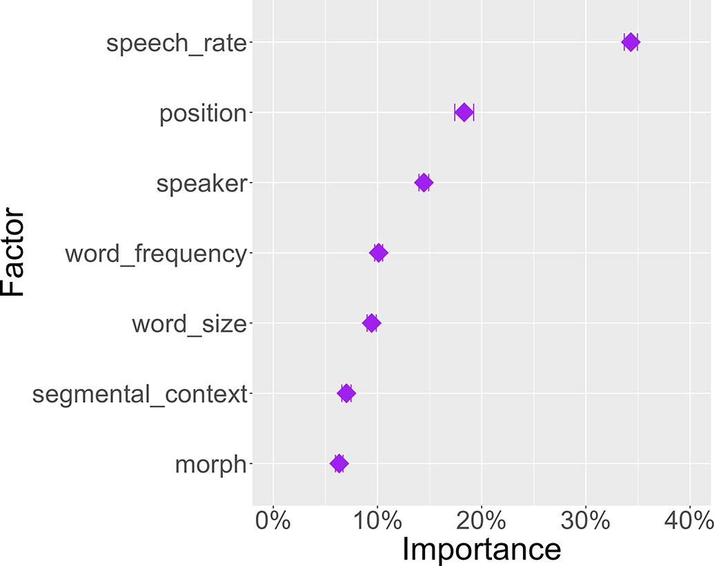
Figure 3 shows the average relative contributions of the seven factors across all languages and homophone sets. By far, the most important factor was local speech_rate at 34.3%. The second most important factor was position at 18.3%, reflecting the well-known process of Final Lengthening. The third most important variable was speaker at 14.5%. Note that the importance of this variable may be underappreciated because some DoReCo datasets contain data from 20 or more speakers, while others contain recordings from only a single speaker. In an ideal scenario with a perfectly balanced corpus, the relative contribution of speaker would possibly be higher. The fourth most important variable was word_frequency at 10.1%. The factor word_size ranked fifth with a contribution of 9.4%.
Average contribution of seven variables for predicting morph duration.

The segmental_context variable had a rather low overall influence on morph duration (7.0%). The low importance of this variable is likely linked to the fact that coarticulation and word boundary effects apply locally, meaning that the significance of segmental context decreases with larger morph sizes. Furthermore, the extent of segmental effects depends heavily on the phonetic and phonological properties of the individual languages. The morphological affiliation of a morph (i.e. the morph variable) had the lowest overall variable importance, with an average contribution of 6.3%. On a general population level, the morphological identity thus only plays a minor role for the acoustic duration of morphs compared to other factors. However, the relative importance of morph differs considerably across languages (Figure 4) and also between individual homophone sets (see Section 4.2). The three languages with the highest average scores in Figure 4 (Arapaho, Kamas, Texistepec Popoluca) are all highly synthetic. Texistepec Popoluca also has the homophone set with the highest overall morph contribution score, which will be discussed in more detail in Section 4.2.
Average contribution of the morph variable across 37 languages.

Figure 4. Long description
The chart features a vertical y-axis labeled Language and a horizontal x-axis labeled Importance of morph with percentage increments of 0, 10, 20, and 30 percent. Data points are represented by purple diamonds with horizontal error bars.
From top to bottom, the languages and their approximate values are:
* Arapaho: 22 percent
* Kamas: 15 percent
* Texistepec Popoluca: 14 percent
* Beja: 9 percent
* Jejuan: 9 percent
* Evenki: 9 percent
* Yali: 9 percent
* Goemai: 8 percent
* Savosavo: 8 percent
* Pnar: 8 percent
* Mojeño Trinitario: 7 percent
* Gorwaa: 7 percent
* Tabasaran: 7 percent
* Baïnounk Gubëeher: 6 percent
* Nafsan South Efate: 6 percent
* Cashinahua: 6 percent
* Daakie: 6 percent
* Sümi: 6 percent
* N||ng: 6 percent
* Hoocąk: 6 percent
* Sanzhi Dargwa: 6 percent
* Northern Alta: 5 percent
* Nisvai: 5 percent
* Kakabe: 5 percent
* Northern Kurdish Kurmanji: 5 percent
* Vera'a: 5 percent
* Bora: 5 percent
* Teop: 5 percent
* Totoli: 5 percent
* Urum: 4 percent
* Movima: 4 percent
* Ruuli: 4 percent
* Cabécar: 4 percent
* Dalabon: 3 percent
* Dolgan: 3 percent
* Jahai: 3 percent
* Fanbyak: 2 percent
The error bars are widest for Kamas and Texistepec Popoluca and narrowest for Arapaho and Fanbyak.
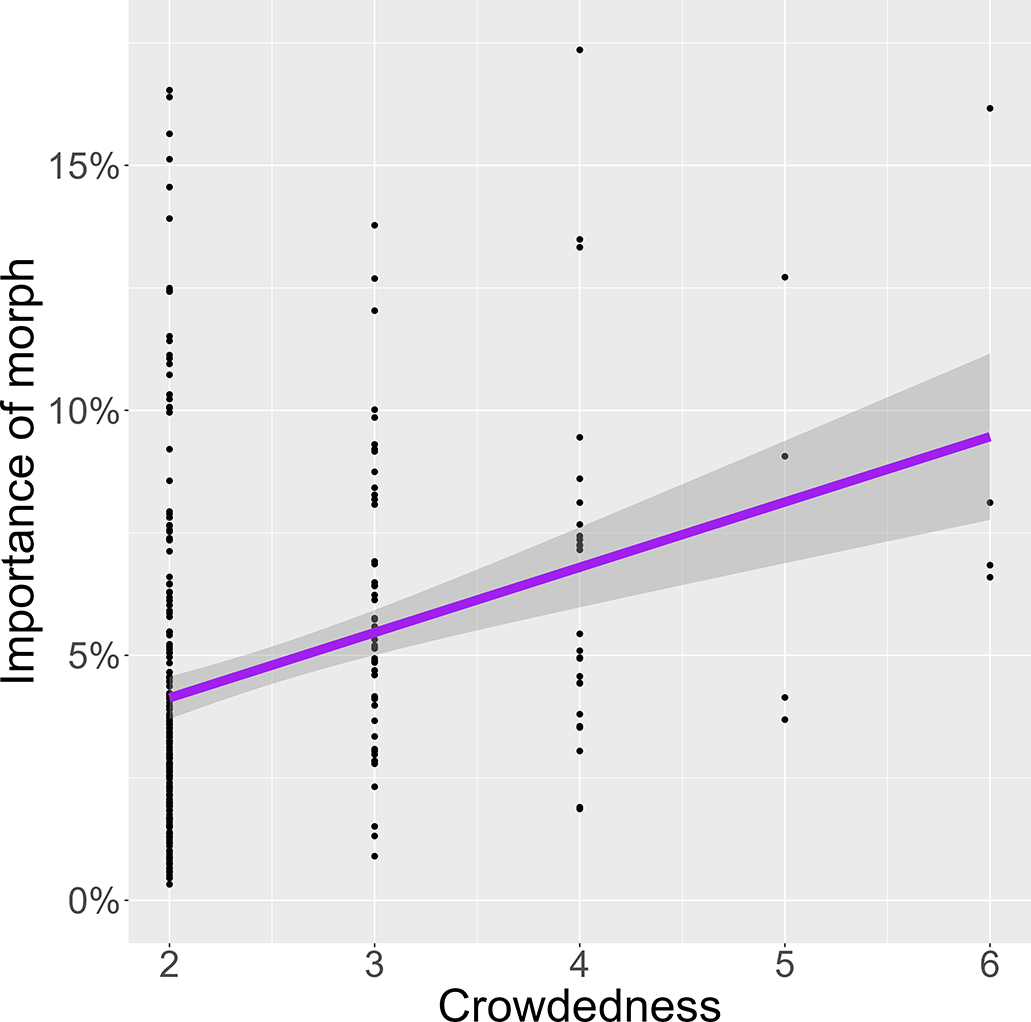
Turning now to the question if homophone sets that resemble the English <s> homophones imply a stronger importance of morph, three independent factors were explored: crowdedness, presence of an alveolar fricative, and homogeneity. The first, crowdedness, indeed affected the importance of the morph variable. Figure 5 illustrates the relation between the size of homophone sets and the weight of the morph variable across all languages in the sample. The overlaid regression line reveals a positive and significant correlation between these two dimensions (R = 0.12, p < 0.05). This can be interpreted such that the more competing homophonous morphs exist in a language, the more their durations are clustered around individual morphs. Note, however, that the number of homophone sets is not equally distributed over the size categories. The majority of homophone sets had two (227/319) members, and sets with three (54/319), four (27/319) or more (11/319) members were increasingly less frequent.
Correlation between crowdedness (homophone set size) and average importance of the morph variable.

Figure 5. Long description
The X axis is labeled Crowdedness with discrete integer values from 2 to 6. The Y axis is labeled Importance of morph with percentage values from 0 percent to 15 percent.
Data points are clustered in vertical columns at each integer on the X axis.
* At Crowdedness 2, there is a high density of points concentrated between 0 percent and 5 percent, with several outliers reaching up to 17 percent.
* At Crowdedness 3, points are more spread out between 1 percent and 14 percent.
* At Crowdedness 4, points are distributed between 2 percent and 18 percent.
* At Crowdedness 5, there are fewer data points, ranging from 4 percent to 13 percent.
* At Crowdedness 6, points are scattered between 7 percent and 16 percent.
A solid purple regression line starts at approximately 4 percent on the Y axis at Crowdedness 2 and rises with a positive linear slope to approximately 9.5 percent at Crowdedness 6. A light gray shaded area surrounds the purple line, representing the confidence interval, which widens as Crowdedness increases from left to right.
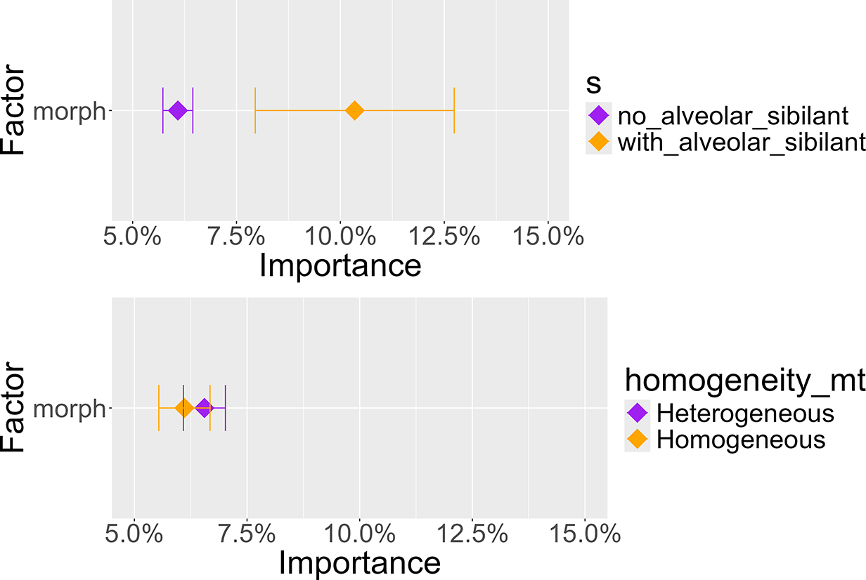
To investigate whether morphs containing an alveolar sibilant are better candidates for the acoustic disambiguation of homophone sets, the data were split into two subsets, one including morphs with at least one alveolar sibilant (in any position), and one including the other morphs. To test whether homophone sets containing only a certain type of morph (roots, suffixes, prefixes, enclitics, proclitics, infixes) are more prone to acoustic differentiation than mixed sets, the data were again split into two subsets, one containing homogeneous homophone sets and the other containing heterogeneous sets. Figure 6 shows the importance of the morph variable across these four subsets. First, there is a clear difference in the average variable importance between homophones with and without an alveolar fricative. Homophones with an alveolar sibilant (orange) had notably lower average importance for morph than homophones without such a fricative (purple), with average scores being 10.3% and 6.0%, respectively. These results should be treated with some caution, though, as the two sets were not equal in size: homophone sets containing an alveolar fricative only made up 5.6% of homophone sets included in the final models. Second, the average morph importance scores for homogeneous and heterogeneous sets were very similar, with values of 6.1% and 6.5%, respectively. The two sets were of almost identical size, with 50.7% being homogeneous.
Variable importance depending on presence of an alveolar sibilant (top) and homogeneity of morph type (bottom).

Figure 6. Long description
A multi-panel figure with two vertically stacked dot plots. Both plots share a horizontal x-axis labeled Importance ranging from 5.0% to 15.0% and a vertical y-axis labeled Factor with a single entry for morph.
Top Panel: Labeled with legend s.
* A purple diamond representing no_alveolar_sibilant is positioned at approximately 6% importance with a narrow error bar.
* An orange diamond representing with_alveolar_sibilant is positioned at approximately 10.5% importance with a wide error bar extending from 8% to 13%.
Bottom Panel: Labeled with legend homogeneity_mt.
* A purple diamond representing Heterogeneous is positioned at approximately 6.5% importance with a narrow error bar.
* An orange diamond representing Homogeneous is positioned at approximately 6% importance with a narrow error bar.
In both panels, the data points are centered on the morph factor line.
The data thus support the initial hypothesis regarding homophones with an alveolar sibilant bearing higher importance for morph, but results are inconclusive regarding the homogeneity dimension.
4.2. Homophone sets with high morph importance
The quantitative analysis has revealed an overall low importance of morphological identity for the acoustic duration of homophones but has also identified factors related to crowdedness and segmental properties that appear to increase the likelihood of morphological disambiguation. As shown in Figure 4, there are considerable differences in the contribution of the morph variable across languages. These differences ultimately boil down to differences between individual homophone sets, some of which display exceptionally high scores for the morph variable. Table 2 lists the 25 homophone sets with the highest morph contributions, ranging from 19% to 41%. A crucial observation is that there is no single language, linguistic family, or area dominating this list. Likewise, the size and shape of the morphs are highly varied, ranging in size from a single segment (such as Northern Alta o) to polysyllabic forms (such as Nisvai likanim). Consequently, there do not appear to be any particular macro-level features interacting with the morph variable.
Top 25 homophone sets with the highest relative importance of the morph variable. Meanings = distinct meanings (glosses) after filtering. Tokens = number of morphs in homophone sets evaluated by the statistical models

Table 2. Long description
The table contains six columns: Rank, Language, Morph, Meanings, Tokens, and Importance.
1. Texistepec Popoluca, morph w ä ä, 2 meanings, 63 tokens, 41% importance.
2. Beja, morph j i, 4 meanings, 62 tokens, 33% importance.
3. Yali, morph s u, 2 meanings, 188 tokens, 32% importance.
4. Kamas, morph k u, 2 meanings, 76 tokens, 31% importance.
5. Savosavo, morph s u a, 2 meanings, 248 tokens, 30% importance.
6. Goemai, morph d apostrophe a, 2 meanings, 140 tokens, 30% importance.
7. Nisvai, morph l i k a n i m, 2 meanings, 27 tokens, 27% importance.
8. Goemai, morph h o k, 2 meanings, 171 tokens, 26% importance.
9. Tabasaran, morph š, 2 meanings, 66 tokens, 26% importance.
10. Vera’a, morph s u, 2 meanings, 88 tokens, 26% importance.
11. Yali, morph t u, 2 meanings, 275 tokens, 24% importance.
12. Mojeño Trinitario, morph o apostrophe i, 2 meanings, 112 tokens, 23% importance.
13. Texistepec Popoluca, morph apostrophe, 6 meanings, 155 tokens, 22% importance.
14. Jejuan, morph t super h a, 2 meanings, 39 tokens, 22% importance.
15. Northern Alta, morph o, 2 meanings, 53 tokens, 22% importance.
16. Daakie, morph t e, 2 meanings, 58 tokens, 22% importance.
17. Arapaho, morph n i h i i, 2 meanings, 45 tokens, 21% importance.
18. Pnar, morph k a m, 3 meanings, 59 tokens, 20% importance.
19. Jejuan, morph t ɕ i, 3 meanings, 64 tokens, 20% importance.
20. Gorwaa, morph e e, 3 meanings, 304 tokens, 20% importance.
21. Kamas, morph k u ʔ, 2 meanings, 24 tokens, 20% importance.
22. Totoli, morph s, 2 meanings, 33 tokens, 20% importance.
23. Evenki, morph a, 2 meanings, 47 tokens, 19% importance.
24. Pnar, morph n o n g, 2 meanings, 20 tokens, 19% importance.
25. Baïnounk Gubëeher, morph d, 3 meanings, 99 tokens, 19% importance.
In the following, five homophone sets will be discussed in more detail, highlighting additional factors that may contribute to the relatively high variable importance for those homophone sets.
4.2.1. Texistepec Popoluca wää
The homophone set wää in Texistepec Popoluca consists of the adjective/adverb ‘good, well’ and the auxiliary verb ‘can(aux)’.Footnote 12 Both the adjective/adverb and the auxiliary wää usually occur on their own, but may occasionally also appear within complex words: the auxiliary may be accompanied by the plural marker -be or the perfective clitic =am, while the adjective is attested in DoReCo within certain compound-like constructions such as wää-dä’ ‘(good) water’. The examples in (3) and (4) show two typical contexts in which these forms are used.
(3)
maas
wää
y<y>oomä’-baa
more[Sp]
good
<3:a>woman-dim
‘His daughter is better.’
[Wichmann Reference Wichmann, Seifart, Paschen and Stave2024, doreco_texi1237_JuanFlojo_part4]
(4)
yoomä’
’eñch
wää
ny-daks
d<y>äm
woman
no
can(aux)
2/3-hit
<3:a>say
‘You can’t hit the woman, he says.’
[Wichmann Reference Wichmann, Seifart, Paschen and Stave2024, doreco_texi1237_LaMujerFloja]
For wää ‘good, well’, 38 tokens with an average duration of 261ms are included in the models, while wää ‘can(aux)’ is attested 25 times with a mean duration of 161ms (Table 3). A plausible explanation for the differences in duration is that content words tend to be generally more phonetically robust than function words. Moreover, evaluative adjectives such as wää ‘good, well’ can be prosodically prominent in emphatic contexts (Selting Reference Selting1994). As the corpus data used here contain spontaneous speech, it is likely that emphatic prosody is used widely, and the marked temporal differences are due to a combination of word class and prosodic factors.
Texistepec Popoluca wää homophone set with average morph durations

Table 3. Long description
The table consists of a single row divided into two main sections comparing the homophone w ä ä.
* The first section on the left lists the word w ä ä, its meaning as ‘good, well’, and an average morph duration of 261 m s.
* The second section on the right lists the word w ä ä, its meaning as ‘can (A U X)', and an average morph duration of 161 m s.
4.2.2. Beja ji
The CV string ji in Beja can be a genitive suffix ‘-gen’, a relative enclitic ‘=rel’, a relative plural masculine proclitic ‘rel.pl.m=’, a first-person singular nominative/accusative possessive marker ‘=poss.1sg.nom/acc’, an aorist tense suffix ‘-aor.3sg.m’, a copula enclitic ‘=cop.3sg’, and an emphatic clitic ‘=emph’ (Table 4).Footnote 13 Only the case suffix, the possessive marker, and the two relative clitics are included in the models, as the other three were not frequent enough in the corpus. (5)–(7) show examples of the genitive suffix, the relative enclitic and the copula marker.
Beja ji homophone set with average morph durations. Grey shading indicates morphs not included in the models due to low token frequency

Table 4. Long description
The table is organized into two side-by-side sections of three columns each.
Left section data:
* Row 1: Morph hyphen j i, labeled G E N, duration 76 m s.
* Row 2: Morph j i equals, labeled R E L dot P L dot M equals, duration 236 m s.
* Row 3: Morph hyphen j i, labeled hyphen A O R dot 3 S G dot M, duration is blank and shaded grey.
Right section data:
* Row 1: Morph equals j i, labeled equals P O S S dot 1 S G dot N O M forward slash A C C, duration 71 m s.
* Row 2: Morph equals j i, labeled equals R E L, duration 107 m s.
* Row 3: Morph equals j i, labeled equals C O P dot 3 S G, duration is blank and shaded grey.
* Row 4: Morph equals j i, labeled equals E M P H, duration is blank and shaded grey.
The Beja ji homophone set is an exceptionally crowded set, similar to English <s>. In addition, there are a number of near-homophonous morphs in Beja, including the two case clitics =jiː ‘abl.sg’ and =jiːb ‘loc.sg’. The situation is further complicated by the fact that all ji morphemes except the relative proclitic attest a shorter i allomorph that lacks the onglide. As [i], [ji] and [jiː] are perceptually close, the perceptual space in the post-stem domain can be assumed to be even more crowded than the list of morphs in Table 4 suggests. Beja ji thus presents a case of an extremely crowded ‘extended’ homophone set, with an exceptionally high number of acoustically similar competing morphs, likely representing a typological rarity.
(5)
hinin
toː=tji
t=asarama
girma-ji
1pl.nom
def.sg.f.acc=serpent
def.f=seven
head-gen
dir-a=b
ni-kati=eːb
kill-cvb.mnr=indf.m.acc
1pl-become\inac=rel.m
‘(We swear) that we killed the seven-headed serpent!’
[Vanhove Reference Vanhove2017: 181]
(6)
baːbija
dibi-a=b
tiː-kti=ji
ptcl
keep-cvb.mnr=indf.m.acc
3sg.f-become\aor
=rel
‘If only you had kept it!’
[Vanhove Reference Vanhove2017: 181]
(7)
haːl=oːkna=ji
state=poss.2pl.acc=
cop.3sg
‘What happened to you? (lit. it is your state)’
[Vanhove Reference Vanhove2017: 206]
4.2.3. Vera’a su
In the Vera’a DoReCo dataset, the morph su occurs in two contexts: as a reduplicative prefix su~ and as a lexical root su ‘to/a paddle’ (Table 5). The latter is a common allomorph of suō; the exact conditions governing the su/suō variation are not entirely clear. The reduplicant su~ mostly appears before su(ō) in the corpus, but cases of su~ occurring before other bases such as sur ‘knit’ are also mentioned in the literature (Schnell Reference Schnell2011: 202).
Vera’a su homophone set

Table 5. Long description
The table consists of six columns in a single row.
* The first column contains the word s u ( o bar).
* The second column provides the English translation ‘paddle’.
* The third column lists a duration of 197 m s.
* The fourth column shows the form s u tilde.
* The fifth column contains the label R E D tilde in small caps.
* The sixth column lists a duration of 114 m s.
Examples (8) through (10) show typical usage examples for su and su~ found in the Vera’a DoReCo dataset. All three examples illustrate reduplicative su~ before su(ō) ‘paddle’ in the same word form. Example (9) showcases su~ occurring in the frequent construction nak su~suō ‘canoe red~paddle’ = ‘canoe (for paddling)’ (cf. Schnell Reference Schnell2011: 71). (10) illustrates an instance of multiple reduplication involving two consecutive su~.
(8)
dir=k
su~su
sar
ma
so=k
’ēn ~’ēn
enteg
sir
3pl=tam2
red
~paddle
inland
hither
nc=tam2
red~see
well
for
‘and as they were paddling up in order to have a good look at (him) […]’
[Schnell Reference Schnell, Seifart, Paschen and Stave2024, doreco_vera1241_veraa_jjq]
(9)
dir’ōl=k
rēv
sur
ēn
nak
su~suō
3tl=tam2
drag
down
art
canoe
red
~paddle
‘The three dragged down a canoe.’
[Schnell Reference Schnell, Seifart, Paschen and Stave2024, doreco_vera1241_veraa_palaa]
(10)
duru=m
su~su~suō
suō
di
sar
ēn
ēre’ie
3DL=TAM1
red
~
red
~paddle
paddle
reach
bushwards
ART
coast
‘The two were paddling, paddled ashore […]’
[Schnell Reference Schnell, Seifart, Paschen and Stave2024, doreco_vera1241_veraa_hhak]
Reduplication inevitably leads to (partial) homophony between base and reduplicant. What is special about this type of homophony is that the two homophones are bound to the same word form. Differences in duration between such homophones likely result from a prosodic asymmetry between base and reduplicant. It should be noted, though, that while about half of the 37 languages in the present sample attest productive reduplication, and reduplicants occur in a total of 16 homophone sets (after filtering), only two homophone sets (Vera’a su and Totoli s) out of the 25 homophone sets with the highest morph importance (Table 2) contain a reduplicant. Phonetic differences between base and reduplicant thus seem to only marginally affect the overall importance of morph.
4.2.4. Arapaho nihii
Arapaho nihii is ambiguous between a verbal root ‘say’ and a discourse particle glossed as ‘well…’ (Table 6). Both morphs have a low tone in the first and a high tone in the second syllable. Verbal nihíí is an intransitive stem that takes an animate subject. There are two formally similar and semantically related applicative verb stems, although they do not seem to be derived from nihíí through synchronically productive means: nihiiθ ‘say/tell to s.o.’ and nihiit ‘say sth.’. The discourse marker nihíí belongs to a closed set of ‘substitutionary or pausal particle[s]’ and is found in contexts of doubt or uncertainty (Cowell & Moss Sr. Reference Cowell and Moss2008: 449).
(11)
kóóxwoow heetkóókohtowúnihíí
koox=woow
e-eti-koon-kohtowu-nihii
again=now
2s-fut-redup-funny/inappropriate-say(ai)
‘I suppose you’re going to say funny things now.’
[Cowell & Moss Sr. Reference Cowell and Moss2008: 199]
(12)
’oh howóó niiyóúno nihíí núhu’ nihíí yóókoxuu.
’oh
owoo
niiyou-no
nihii
nuhu’
nihii
yookox-ii
and
also
here.is-pl
well
this
well
willow-pl
‘And also there were, well, these, well, willows.’
[Cowell & Moss Sr. Reference Cowell and Moss2008: 316]
Arapaho nihii homophone set

Table 6. Long description
The table consists of six columns organized into two comparative sets of three.
Set one (left side):
* Word: nihii
* Meaning: ‘say’
* Duration: 288 m s
Set two (right side):
* Word: nihii
* Meaning: ‘well...’
* Duration: 484 m s
The difference in duration between the two nihíí homophones (ca. 200ms on average) is substantial, and can at least be partially attributed to word size: verbal nihíí tends to occur within complex polymorphemic word forms whereas the particle nihíí only appears in isolation, cf. (11) and (12). As word_size is included as a factor in the models, the fact that morphological identity still substantially contributes to predict the duration of these morphs remains somewhat mysterious. The sheer magnitude of durational differences may have boosted the importance of the morph variable. Another potential explanation could be the floating H tone of verbal nihíí, which usually attaches to the preceding tone-bearing unit and thus influences the tonal properties of the whole stem, potentially leading to systematic differences in acoustic duration.Footnote 14
4.2.5. Banounk Gubëeher d
The Baïnounk Gubëeher d homophone set has three members: the negative perfective/irrealis suffix -d ‘-neg:perf’, the negative future/habitual prefix d- ‘neg:fut-’, and the benefactive suffix -d ‘-ben’. These are also the only three d morphs attested in the Baïnounk Gubëeher DoReCo dataset (Table 7). Both the benefactive suffix and the negative perfective suffix occur 20 times in the data sample, while the negative future prefix is attested 59 times.
Banounk Gubëeher d homophone set

Table 7. Long description
The table consists of two rows and six columns.
Row 1:
- Column 1: hyphen d
- Column 2: hyphen N E G colon P E R F
- Column 3: 38ms
- Column 4: hyphen d
- Column 5: hyphen B E N
- Column 6: 32ms
Row 2:
- Column 1: d hyphen
- Column 2: N E G colon F U T hyphen
- Column 3: 65ms
- Column 4: Empty
- Column 5: Empty
- Column 6: Empty
(13) and (14) provide examples of the two negative markers, and (15) illustrates the use of the benefactive suffix -d.
(13)
me
g-u-cil-ex
indan
bi-na’-hen
d-ë-bun
1sg
foc.obj–2-laugh-hab
go:imp
cl.bi-way-2sgposs
neg:fut-3-good
‘You are laughing about me? Go, your journey will not be successful.’
[Cobbinah Reference Cobbinah2013: 244]
(14)
me
wul-aa-d-i (< wul-aar-r-i)
1sg
see-already
-neg:perf
-1sgsubj
‘I have never seen that!’
[Cobbinah Reference Cobbinah2013: 245]
(15)
a-yen-eneŋ
a-n-dú-d-ët-om
3-say-3pl.obj
3-pl-draw.water
-ben-ven–1sg.obj
‘They told them to fetch them some.’
[Cobbinah Reference Cobbinah, Seifart, Paschen and Stave2024, doreco_bain1259_DJI070211AC]
A crucial observation about the two negative affixes is that the future prefix is underlyingly /d/ but the negative perfective suffix is underlyingly /r/, with a predictable allophone [d] after stems ending in /n/ and /r/ (Cobbinah Reference Cobbinah2013: 231). This allophony is instantiated by two regular phonological processes in the language: fortition of /r/ to /d/ after /n/ and /r/, and subsequent deletion of the first /r/ (Cobbinah Reference Cobbinah2013: 173). It is plausible that the negative perfective -d shows a slightly longer duration because it still retains traces of the two underlying segments it is derived from, even though a difference of 7ms is unlikely to be perceptually relevant. The longer duration of the negative future prefix d-, which often occurs word-initially in Baïnounk Gubëeher (13), may be linked to the process of word-initial lengthening (Blum et al. Reference Blum, Paschen, Forkel, Fuchs and Seifart2024).
5. Discussion
5.1. General discussion
Homophony is a common phenomenon in the world’s languages, and in the present study, this is reflected by the fact that even after applying several layers of filters, languages in the 37-language sample had an average of eight to nine distinct homophone sets (Table 1). Once a broad cross-linguistic perspective is adopted, the role of morphological identity in explaining acoustic differences between homophones turns out to be far less impactful compared to previous reports based on languages such as English or German. It appears that most homophone sets in most languages do not pose any communicative challenge and therefore do not prompt any sub-phonemic durational cues to their lexical identity. And indeed, it is difficult to construe a scenario in which an interlocutor is unable to infer from the communicative context whether a speaker intended to say time or thyme, for instance.
Previous studies have pointed out that acoustic differences between certain homophones can readily be explained by frequency or prosodic factors, prompting the question how meaningful morphological identity is in shaping the acoustic form of homophones. While prosodic factors (speech rate and position) and word frequency had a consistently high impact on the duration of morphs in the present study, the strength of the relative contribution of morphological identity varied considerably across homophone sets. Three properties of homophone sets were tested specifically as to whether they made homophonous morphs more susceptible to acoustic disambiguation.Footnote 15
First, the crowdedness of the homophone space was found to correlate with the relative importance of morphological identity. Homophone sets with more members showed a tendency to display higher morphological contribution scores than homophone sets with fewer members. The majority of homophone sets had two or three members, while sets with four or more members were uncommon. A possible interpretation of these facts is that languages tend to avoid crowded homophone sets, but when they occur, languages may selectively employ subtle durational differences to disambiguate segmentally homophonous morphs.
Second, the presence of an alveolar sibilant increased the average importance of the morphological identity variable. The fricative /s/ is one of the perceptually most salient sounds, and is notorious in sociophonetic research for being the carrier of various non-lexical meanings. It stands to reason that certain segments are more prone than others to express communicative nuances by sub-phonemic detail. The acoustic salience of /s/ appears to contribute to its importance in differentiating homophones by means of acoustic duration.
Third, homogeneity of morph type did not show any notable effect on the importance of lexical identity. It did not matter whether all members in a homophone set were of the same morph type (e.g. all suffixes) or whether sets were mixed. This suggests that there is no a priori acoustic advantage of root material over affix or clitic material, as would be expected from the phonological literature, but also from previous studies such as Plag et al. (Reference Plag, Homann and Kunter2017), who found that root segments were longer than most affix segments, which in turn were longer than clitic segments in English. This negative result further suggests that positional effects (e.g. the fact that suffixes undergo Final Lengthening more often than prefixes) may nullify the effect of morphological identity in mixed homophone sets.
Lastly, there may be additional features within individual homophone sets that further influence to what degree acoustic differences between homophones are driven by morphology. These features include word class, as in the case of Texistepec Popoluca wää; the distinction between underlying vs. derived segments, as in the case of Baïnounk Gubëeher d; and morphological interdependence, as in the case of Vera’a su, where the two homophones often occur as base and reduplicant within the same word form.
5.2. Implications for theories of grammar
The results align with functional theories of grammar that view languages as adaptive systems shaped primarily by the goal of efficient communication (Nichols Reference Nichols1984, Croft Reference Croft, Geeraerts and Cuyckens2010, Levshina Reference Levshina2023). The general low importance of morphological identity in explaining acoustic differences between homophonous morphs can be seen as avoiding additional articulatory and cognitive effort, as in most cases, homophones can easily be disambiguated through context. This has also been observed in language acquisition, where homophones that are distributed across syntactic and semantic categories did not pose a learning challenge for children (Dautriche et al. Reference Dautriche, Fibla, Fievet and Christophe2018). In highly crowded homophone sets, the risk of confusion increases, making phonetic differentiation more beneficial. As certain segments such as /s/ are particularly well-suited to differentiate meanings, homophones with such segments are also more prone to show systematic acoustic differences. Against this background, the results reported for English <s> can be understood as an adaptation to phonetically disambiguate otherwise homophonous morphs catalyzed by independent factors related to the shape and structure of this particular homophone set. This situation is paralleled by certain other homophone sets such as Beja ji but is not the default scenario in the sample studied here.
The role of crowdedness as a crucial factor in predicting temporal differences between homophones appears to be in line with the idea of discriminative learning and the discriminative lexicon (Chuang & Baayen Reference Chuang and Baayen2021). When a form corresponds to multiple meanings, competition arises in the mental lexicon as acoustic cues are used to resolve ambiguity and predict the correct meaning. Durational differences, by making homophones acoustically distinct, reduce this competition and facilitate more accurate form-to-meaning mapping during comprehension. This resonates with results reported in Tomaschek et al. (Reference Tomaschek, Plag, Ernestus and Baayen2021), who demonstrated that naïve discriminative learning effectively predicts the durational variation of English <s> morphs based on contextual and morphological features. Similarly, Schmitz et al. (Reference Schmitz, Plag, Baer-Henney and Stein2021) showed that linear discriminative learning models capture morpho-phonetic effects even in pseudowords.
As far as formal theories of grammar are concerned, Plag et al. (Reference Plag, Homann and Kunter2017) make the argument that their findings regarding English <s> homophones challenge modular feed-forward theories of grammar. In these frameworks (Kiparsky Reference Kiparsky1985, Bermúdez-Otero Reference Bermúdez-Otero and Trommer2012), morphological information is assumed to be inaccessible to phonology and phonetics due to an operation called bracket erasure, or phonetization in Colored Containment (Trommer Reference Trommer2011). Consequently, sub-phonemic fine-tuning based on information stored in the lexicon has no straightforward explanation in those frameworks. While the acoustic disambiguation of homophones appears to be a rather weak factor for most languages investigated in the present study, some homophones, including English <s>, showed a considerable effect of morphological identity on acoustic duration. This raises the question of how those sub-phonemic differences can possibly be accounted for in formal theories of grammar.
In theories where information on morphological affiliation is not accessible after spell-out, it is possible to encode subphonemic detail directly in the lexicon.Footnote 16 Whether this information includes timing gestures, articulatory targets, or simply richer phonological representations depends largely on the chosen framework. In Q theory (Garvin et al. Reference Garvin, Lapierre and Inkelas2018, Shih & Inkelas Reference Shih and Inkelas2019), otherwise homophonous members of a homophone set could be lexically specified as differing in their subsegmental composition. While segments are usually made up of three subsegments, Q Theory has a provision allowing temporal flexibility by assigning certain segments a lower or higher number of subsegments. Another strand of research, the theory of Gradient Symbolic Representations, suggests that phonological elements can vary in their levels of presence within an underlying representation (Zimmermann Reference Zimmermann2019). The activity of segments or prosodic nodes can be quantified numerically. For example, two homophones could have slight differences in the underlying activity of certain segments or prosodic nodes associated with those segments, resulting in subtle acoustic differences. Thus, models that allow rich phonological representations obviate the need for morphological look-up in accounting for sub-phonemic acoustic differences.
Lastly, differences in duration could also be the result of different prosodic structures in the lexicon. Plag et al. (Reference Plag, Homann and Kunter2017) do acknowledge this possibility but dismiss this proposal as not applicable to the various <s> homophones in English (see also Schmitz et al. Reference Schmitz, Plag, Baer-Henney and Stein2021). While a convincing analysis of the English data in terms of prosodic structure is yet to be presented, there is no reason why a prosodic account could not work for other homophone sets in other languages. As has been demonstrated in the literature, differences in prosodic specifications can explain otherwise unexpected phonological and morphological patterns (McCarthy & Prince Reference McCarthy and Prince1986, Saba Kirchner Reference Saba Kirchner2013, Zimmermann Reference Zimmermann2017). This avenue appears especially promising for heterogenous homophone sets under the condition that independent evidence exists for differences in the amount of prosodic structure between roots, clitics, and affixes.
5.3. Limitations
While the present study encompasses a wide range of typologically diverse languages and considers various factors known to affect morph duration, there are certain limitations inherent to the study design and data that need to be addressed.
Apart from the variables included in this study, there are other factors known to influence segmental duration that could not be considered here for various reasons. One such factor is prominence, be it in the form of word-level stress or as phrasal accent under focus. Unfortunately, annotations of prominence are not part of the DoReCo datasets, and the details of word- and phrase-level prosody are still not fully understood for many languages in the sample. Another potentially meaningful variable is predictability, which is a more fine-grained measure to predict phonetic reduction than token frequency, which was employed in this study. Predictability takes into consideration the local context in which a word appears and requires large corpora, as well as a deeper understanding of the grammar of a given language (Kliegl et al. Reference Kliegl, Grabner, Rolfs and Engbert2004, Lee et al. Reference Lee, Liu and Tsai2012, Tang & Bennett Reference Tang and Bennett2018).
The present study focused on segmental homophones, based on the annotations on the morpheme break tier in the DoReCo corpus. However, as mentioned in Section 4.2, some of the languages in DoReCo are tone languages, which means that segmentally homophonous morphs may differ in their tonal make-up, which, in a strict sense, would deprive them of their status as homophones. In addition, some languages are lexical stress languages, which means that two segmentally homophonous morphs may consistently differ in stress placement. In the 37-language sample, seven languages can with some certainty be classified as tone languages and 16 languages as lexical stress languages. At first glance, tone languages and languages with lexical stress seem to be neither over-represented nor under-represented in the list of homophones with high morph importance scores in Table 2. Nevertheless, taking into account more information on prosodic features in cross-linguistic studies of homophones would be desirable in future research.
A methodological difference between this study and studies such as Plag et al. (Reference Plag, Homann and Kunter2017), Seyfarth et al. (Reference Seyfarth, Garellek, Gillingham, Farrell and Malouf2017) or Zuraw et al. (Reference Zuraw, Lin, Yang and Peperkamp2021) is that the present study is concerned with homophonous morphs but not parts of stems or complex full words that are homophonous with freestanding word forms. While it would be in theory possible to automatically compare homophonous strings smaller or larger than a single morph, interpreting the results over a large sample of typologically diverse languages could prove to be challenging. It appears a more sensible approach would start with an informed pre-selection on an individual language basis and then incrementally build up a reasonably sized sample for comparison. This will hopefully be possible in the future as more annotated and time-aligned data for endangered and understudied languages become available.
6. Conclusion
Do speakers systematically use fine phonetic details to distinguish segmentally homophonous morphs? Based on annotated spontaneous speech data from 37 languages, the answer appears to be ‘no’, at least on a broad scale. While homophones often exhibit differences in acoustic duration, those differences are only minimally influenced by their homophonic nature. Instead, factors such as speech rate and frequency are significantly stronger predictors. As most homophones do not present communicative challenges, it is generally unnecessary to enhance their acoustic distinction. However, in exceptional cases where there is a crowded homophone space with multiple competing meanings and the segmental composition allows for phonetic fine-tuning, speakers may selectively differentiate homophones based on their temporal duration. In these instances, disambiguating homophones through additional articulatory effort seems to benefit efficient communication. These findings provide a framework for understanding the well-known case of English <s> and contextualize it in a wider cross-linguistic perspective.
Acknowledgements
This research was supported by a grant from the German Research Foundation to Ludger Paschen (DFG-PA2368/1-1). I want to thank the audiences of the ‘Mismatches and Disambiguation’ group at ZAS Berlin and the members of the Potsdam Morpho-Syntax Lab for helpful comments and feedback. I am grateful to Aleksandr Schamberger for his support at various stages of this study. I thank three anonymous reviewers for their suggestions and constructive criticism. I am especially grateful to Nicholas Rolle, Matt Stave and Frank Seifart for previous discussions about homophony in the context of the DoReCo corpus, which partially inspired this study. All errors remain my own.
Appendix
This appendix includes information on four alternative models that use a slightly different array of variables or model structures. It also discusses whether dataset size may influence the importance of the morph variable.
Reversed model
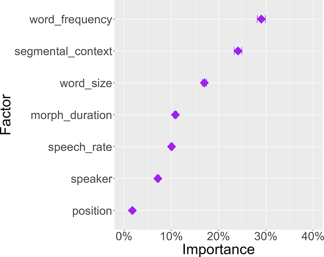
It is in principle possible to construct a reversed model that predicts morphological identity from morph duration. The variable importance scores of such a ‘flipped’ model is given in Figure 7. The figure shows that morph_duration is slightly better at predicting morphological identity than vice versa, with an importance of ca. 11%. The order of the other factors is almost reversed compared to the original model, with word_frequency and segmental_context having high and position and speaker having low contribution values. These results are not surprising given that this is a reversed model.
Average contribution of seven variables for predicting morphological identity in a ‘flipped’ model.

Figure 7. Long description
The dot plot features a vertical Y axis labeled Factor and a horizontal X axis labeled Importance with a scale from 0% to 40%. Seven factors are represented by purple diamond markers with horizontal error bars, ordered from highest to lowest importance.
* word_frequency is at approximately 29%.
* segmental_context is at approximately 24%.
* word_size is at approximately 17%.
* morph_duration is at approximately 11%.
* speech_rate is at approximately 10%.
* speaker is at approximately 7%.
* position is at approximately 2%.
Model without the speaker variable
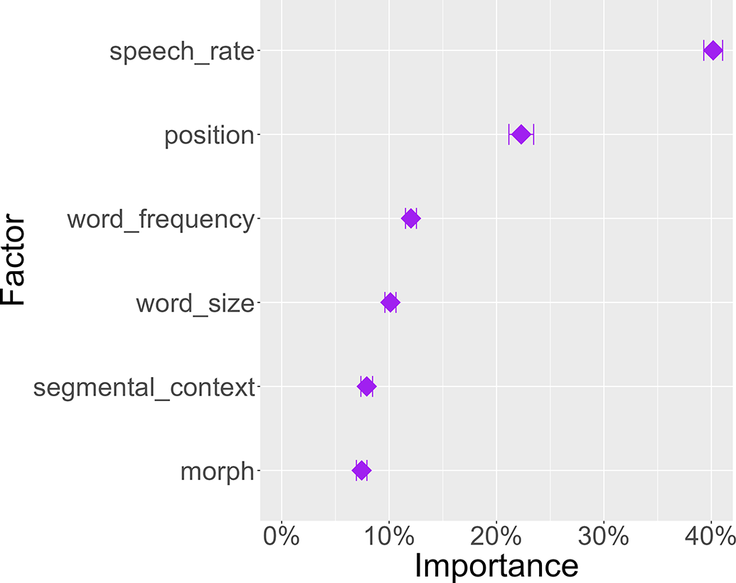
As noted in Section 4.1, DoReCo is not balanced when it comes to the speaker variable, and datasets differ dramatically in how many speakers they contain. The variable importance scores of a model that does not include the factor speaker is given in Figure 8. The ranking of the factors is identical to the one in the model described in Section 4 (Figure 3), indicating that the unbalanced nature of the speaker variable does not skew the model in any direction.
Average contribution of six variables (without speaker) for predicting morph duration.

Figure 8. Long description
The horizontal x axis is labeled Importance and ranges from 0 percent to 40 percent in increments of 10 percent. The vertical y axis is labeled Factor and lists six variables. Data points are represented by purple diamonds with horizontal error bars.
From top to bottom, the factors and their approximate importance values are
* speech underscore rate at 40 percent.
* position at 22 percent.
* word underscore frequency at 12 percent.
* word underscore size at 10 percent.
* segmental underscore context at 8 percent.
* morph at 7 percent.
Model with extended segmental context information
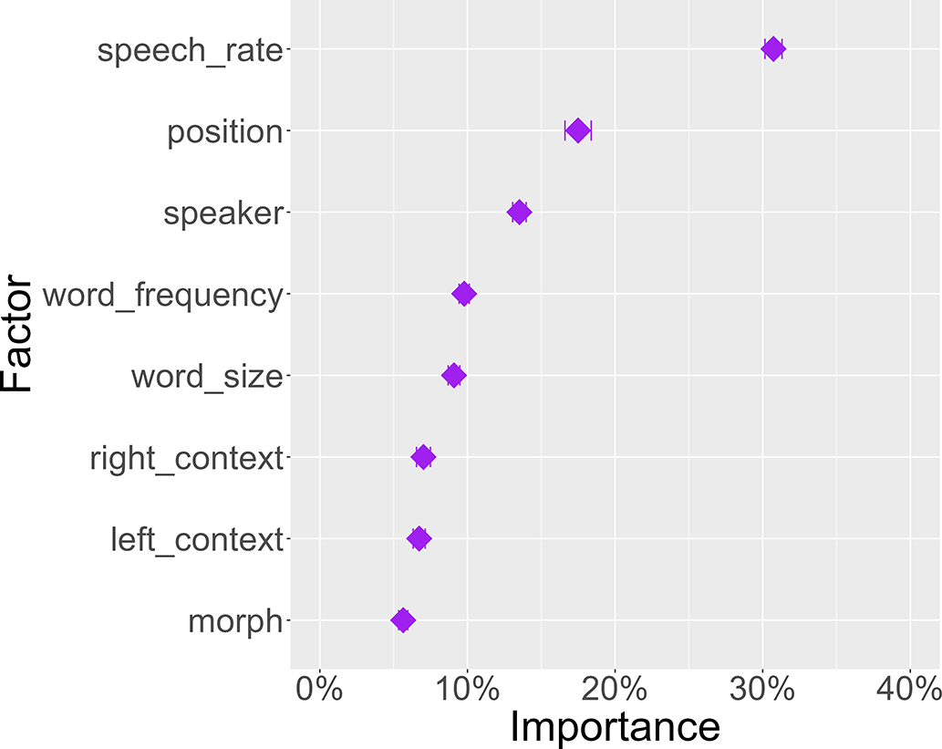
Figure 9 shows a model in which segmental_context is split into left and right context and encodes the individual segments rather than broad groups of segments. In such a model with maximum information on segmental context, the two granular context factors are virtually identical to the broad segmental_context factor from the model described in Section 4 in terms of their relatively low contribution scores and their ranking barely above morph.
Average contribution of eight variables for predicting morph duration.

Figure 9. Long description
The horizontal X-axis is labeled Importance and ranges from 0% to 40% in increments of 10%. The vertical Y-axis is labeled Factor and lists eight variables. Purple diamond markers with small horizontal error bars indicate the importance value for each factor.
From top to bottom, the factors and their approximate values are
* speech_rate at 31%
* position at 18%
* speaker at 14%
* word_frequency at 10%
* word_size at 9%
* right_context at 7%
* left_context at 7%
* morph at 6%
Model with an additional morph_type factor
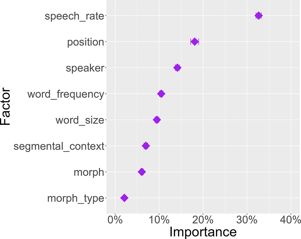
Figure 10 shows a model with an additional morph_type variable. Intuitively, one might expect this variable to be highly informative, as phonological and phonetic differences between roots, clitics and affixes affecting their duration have been described in the literature (Beckmann Reference Beckmann1998, Plag et al. Reference Plag, Homann and Kunter2017). However, morph_type has a variable importance of close to 0%. The reason is that there is an implicational relation between morph and morph_type whereby each morph has exactly one value for morph_type, and in any given homophone set, the maximum number of categories for morph_type depends on morph (but not vice versa).
Average contribution of eight variables for predicting morph duration.

Figure 10. Long description
The dot plot features a vertical Y axis labeled Factor and a horizontal X axis labeled Importance with a scale from 0% to 40% in increments of 10%. Eight purple diamond-shaped data points with horizontal error bars are plotted from top to bottom in descending order of importance.
* speech_rate is at approximately 33%.
* position is at approximately 18%.
* speaker is at approximately 14%.
* word_frequency is at approximately 10%.
* word_size is at approximately 9%.
* segmental_context is at approximately 7%.
* morph is at approximately 6%.
* morph_type is at approximately 2%.
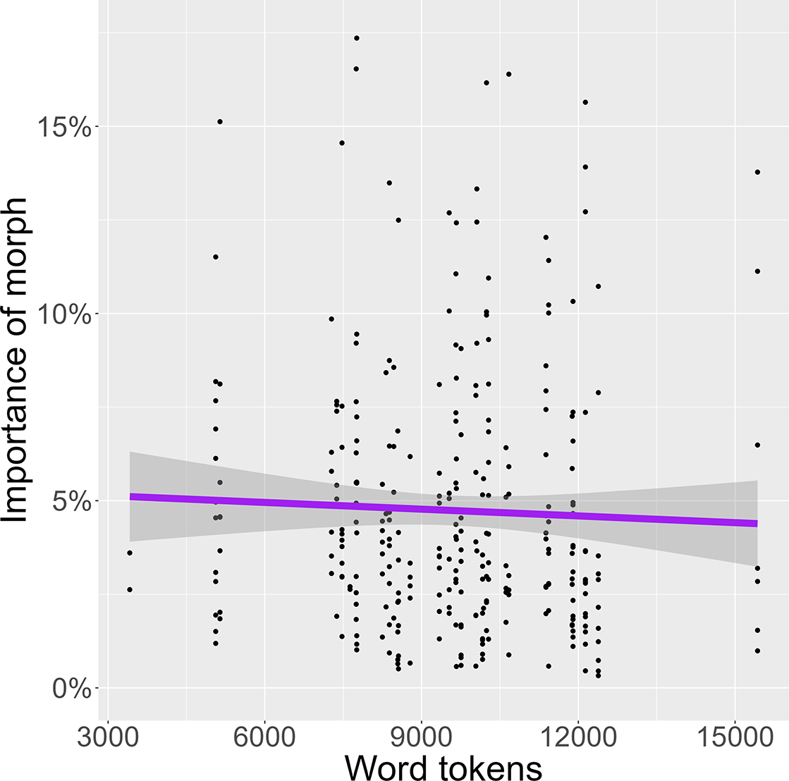
The relation between dataset size and the morph variable
Figure 11 shows the relation between dataset size (in word tokens) and the importance of morph. No meaningful interaction between these two parameters is visible, and linear regression reveals a lack of a significant correlation (R = -0.03, p = 0.52).
The relation between word tokens (per dataset) and the importance of morph.

Figure 11. Long description
The x-axis is labeled Word tokens with numerical increments at 3000, 6000, 9000, 12000, and 15000. The y-axis is labeled Importance of morph with percentage increments at 0 percent, 5 percent, 10 percent, and 15 percent. The data is presented as a scatter plot of black dots clustered primarily between 7000 and 13000 word tokens. While most points are concentrated below the 10 percent mark, several outliers reach as high as 17 percent. A solid purple regression line is overlaid on the data, showing a very slight downward trend from approximately 5 percent at 3000 tokens to just below 5 percent at 15000 tokens. A light gray shaded area surrounds the purple line, representing the confidence interval, which widens slightly at the far left and right ends of the x-axis.










 Open access

