1. Introduction
Several policy measures have been adopted worldwide to dampen the severe effects of the COVID-19 pandemic crisis on economic and financial activities. Central bank interventions, government support measures, and supervisory/regulatory action helped mitigate this economic and financial impact to a large extent. Although the financial system has entered the COVID-19 pandemic crisis with high resilience, the risks posed by the pandemic remained elevated. In particular, vulnerabilities related to the deterioration of credit quality of nonfinancial borrowers could increasingly affect banks and, more generally, the supply of financing to the real economy (Financial Stability Board, 2020).
In Europe, the policy package approved by the Single Supervisory Mechanism of the European Central Bank (hereafter ECB/SSM) included two measures specifically targeting the banking sector. First, in March 2020 the micro- and macro-prudential authorities allowed for a temporary relaxation of the requirements regarding the Pillar 2 Guidance and the Combined Buffer Requirement (henceforth the flexibility measure).Footnote 1 The main goal of this measure was to support banks to continue to fulfill their role in funding the real economy in the face of significant economic effects of the COVID-19 pandemic. Second, at the end of the same month, another measure was taken and concerned the recommendation not to pay dividends and refrain from buying back shares (henceforth dividends pay-out restriction).Footnote 2 According to the ECB/SSM, this measure aimed at preserving banks’ capacity to absorb losses and support the economy in an environment of exceptional uncertainty. This extraordinary and temporary recommendation helped strengthen the temporary relief in capital requirements. The prudential measures, together with other government and monetary policy measures, prevented potential deleveraging resulting from banks’ procyclical behavior, ensuring the maintenance of an adequate flow of credit to the economy.
In July 2020 the ECB/SSM announced that it would not require European banks to start rebuilding their capital buffers, at least until the end of 2022.Footnote 3 This decision was intended to ensure that the banking system would contribute to a sustainable economic recovery. In February 2022, the ECB/SSM confirmed the path for the capital replenishment and that, therefore, it would not extend capital relief for banks beyond the end of 2022.Footnote 4 All the aforementioned measures were also applied to less significant institutions in Portugal, following the decisions taken by Banco de Portugal.Footnote 5
During the pandemic, Portuguese banks were allowed to operate temporarily below the regulatory capital, due to the flexibility measure. To some extent, Portuguese banks have used this temporary flexibility. Avezum et al. (Reference Avezum, Vítor Oliveira and Serra2021) find evidence that Portuguese banks with greater headroom above the overall capital requirement granted more credit to firms in the aftermath of the pandemic than banks with lower headroom. Nevertheless, the noncompliance with part of the regulatory capital was still subject to restrictions on dividends distribution, which may explain why some banks have not used the flexibility measure in a more formal way. In fact, other reasons can be argued to explain this behavior, as, for example, market pressure, increased risk aversion by banks or the procyclical effects on lending that may happen due to the expected rebuilding of capital buffers, especially when insufficient information on losses incurred by banks are available.
The enhanced resilience of the European financial system in the run-up to the crisis—defined as the banking sector’s ability to absorb shocks such as economic downturns, market disruptions, or operational risks while maintaining its core functions of credit provision, payment facilitation, and preserving solvency, liquidity, and public confidence—was a key factor in the sector’s responsiveness (Villeroy de Galhau et al. Reference Villeroy de Galhau, De Guindos, Makhlouf, Portes, Dixon, Shin, ElBerger, Avdjiev, Buch, Goldberg and Bussière2021). This enhancement increased the ability to absorb unexpected losses but also the space for macroprudential policy action in crises, as intended.
Once the pandemic crisis is overcome, the rebuilt of capital buffers should be a priority for policymakers. Nonetheless, policymakers should carefully assess the banking sector conditions, to avert procyclical effects on lending of the measures withdrawal. The rebuilding of buffers should be carried out after the recovery process is completed and acknowledging the potential lack of information on potential credit losses incurred by banks over the crisis. The magnitude of procyclical effects will depend, among other factors, on the size of banks’ management capital buffers (i.e., the level of capital buffers above the requirements set by supervisory authorities) and the actions taken by banks to comply with required higher buffer levels. These latter actions include equity issuance, deleveraging, reducing the management capital buffer, or a combination of the three possible strategies. For these reasons, the adoption of different paces and periods for the transition to the precrisis level of capital buffers may be relevant in terms of the impact on financial stability and economic recovery.
This paper aims at (i) assessing the economic and financial impacts of the flexibility measure and the dividends pay-out restriction over the COVID-19 pandemic crisis, and (ii) understanding the implications for financial stability and economic activity of different periods and paces for the gradual rebuilding of capital buffers (henceforth the replenishment of capital buffers). The focus of this assessment is to understand, from a theoretical perspective, whether the implementation of these policy measures are effective in attaining their own objectives. These measures can be seen as a test to the efficacy and effectiveness of macroprudential policy. Evaluating the effects of these two policy measures on the financial system and the impact of their withdrawal enhances our knowledge about the functioning of macroprudential policy, as it can contribute to a more effective use of the macroprudential toolkit to ensure financial stability. The analysis is therefore centered in this period of broadly two years and does not intend to explain the effects of prudential regulation and structural changes on the Portuguese banking system before the pandemic crisis hit.
For these purposes, we use a dynamic stochastic general equilibrium model (DSGE) where banks, impatient households, and entrepreneurs can default, based on Clerc et al. (Reference Clerc, Derviz, Mendicino, Moyen, Nikolov, Stracca, Suarez and Vardoulakis2015) and calibrated for the Portuguese economy, in line with Lima et al. (Reference Lima, Maia and Pereira2023). In this model, micro- and macro-prudential capital requirements play a role in mitigating the financial distortions. Capital buffers are central to our assessment of banking system resilience, as they provide banks with the necessary loss-absorbing capacity, which we proxy using the default probability measure.
To the extent of our knowledge, this work represents the first attempt to assess the impact of the flexibility measure combined with the dividends pay-out restriction, and different replenishment periods for capital buffers for Portugal. More generally, this is one of the first papers analyzing the combined effect of the flexibility measure and the dividends pay-out restriction in a COVID-19 pandemic context. Muñoz (Reference Muñoz2021) represents the closest reference in this regard, as the author shows in a DSGE model how jointly calibrated dividends restriction and the countercyclical capital buffer (CCyB) improve the effectiveness of macroprudential capital measures in smoothing the financial and the business cycle when financial shocks hit the economy.Footnote 6
The work in Dautović et al. (2023) also serves as a benchmark for our results, as authors find that the COVID-19 dividends pay-out restriction positively impacted lending to financially constrained firms, increased capital space for banks, and reduced procyclical behaviors. Moreover, our work is among the first ones to address the replenishment of capital buffers,Footnote 7 and specifically the issue of exploring different path regimes for the replenishment of capital buffers. Darracq Pariès et al., Reference Darracq Pariès, Sørensen and Rodriguez-Palenzuela2011) first approach this topic, highlighting the importance of smoothing out the transition to new (higher) capital requirement levels. The analysis developed in Budnik et al. (Reference Budnik, Pariès, Kok, Lang, Duca, Rancoita, d’Acri, Ryan and Rottner2020b) is more in line with our work, as it quantifies the effects of four different replenishment scenarios using a mix of three different micro- and macro-models.Footnote 8 The authors find that replenishing capital buffers too early or too aggressively could prolong the economic downturn. Consequently, weaker macroeconomic conditions would recommend a later and more gradual restoration of capital buffers.
Our work leads to conclusions in line with the aforementioned literature. First of all, when we consider the application of both the dividends pay-out restriction and the flexibility measure, the beneficial effects on credit and GDP are higher than in the case where only the flexibility measure is applied. Over a three-year period, the two policy measures together cumulatively mitigate credit and GDP losses by 48.4% and 2.7%, respectively. Moreover, the dividends pay-out restriction allows banks to avoid using the flexibility measure entirely, with desirable consequences on banks’ default rate. This result also implies a smaller effort for banks to replenish capital buffers, that is, to return to the preflexibility-measure level of capitalization.
Second, by focusing on the effects of the flexibility measure only, we find that it is still beneficial in its own right. This measure limits the transmission of the COVID-19 pandemic shock to the economy, as it mitigates the negative impact on credit granted to both firms and households. It is especially useful for corporate loans, inducing higher corporate investment. The better ability of the banking sector to finance the economy translates into a milder reduction in GDP in the short-to-medium term and overall in the simulation sample considered. We find that, over a three-year period, the flexibility policy measure helps mitigate credit and GDP losses by 39.4% and 1.2%, respectively. In this assessment, we assume that banks are able to fully use the flexibility measure, without any restrictions. However, as stressed in the ESRB (2021) report, banks might not always be able or willing to use their buffers. The ability or willingness of banks to use capital buffers may depend on several factors, including overlap with other minimum requirements and stigma effects.
Finally, analyzing different transition paths for the replenishment of capital buffers, we conclude that the choice depends on policymakers’ priorities, as it presents trade-offs. Shorter transition horizons are better at strengthening the banking system resilience, while longer time horizons maintain a higher flow of credit to the economy. This evidence is robust to linear and nonlinear specifications of the replenishment paths, even though, in the nonlinear path regime, the differences in the responses for each transition period shrink as horizons extend.
The remaining of this paper is organized as follows. Section 2 frames our work in the current COVID-19-related economic literature, Section 3 summarizes the main features of the model and Section 4 describes the calibration we use. The results for the impact of the flexibility measure and the dividends pay-out restriction are presented in Section 5, while the implications of different replenishment periods for capital buffers are discussed in Section 6. Section 7 reports a sensitivity analysis on the magnitude of the results. Finally, Section 8 concludes.
2. Literature review
Our paper can be traced back to the growing literature concerning the impacts of the COVID-19 pandemic on the economy and the attenuating role of the policy measures put in place in response to it. COVID-19 pandemic was detrimental to several economic sectors, eroded the productivity and profitability of firms, and exposed them to a higher risk of bankruptcy overall (Augusto et al. Reference Augusto, Marques and Martinho2022; Cella, Reference Cella2020; Bloom et al. Reference Bloom, Bunn, Mizen, Smietanka and Thwaites2020). Some empirical evidence focuses on the impact of the mitigating policies implemented by governments on households and firms. MacGee et al. (Reference MacGee, Pugh and See2022) analyze the effects of the pandemic on household debt and unplanned savings in Canada and suggest that the implemented policies have only partially achieved their aim to sustain household consumption. Ebeke et al. (Reference Ebeke, Jovanovic, Valderrama and Zhou2021) argue that corporate sector policy measures have significantly curbed liquidity shortfalls, layoffs, and output losses of European firms. Guth et al. (Reference Guth, Lipp, Puhr and Schneider2020) and De Socio et al. (Reference De Socio, Narizzano, Orlando, Parlapiano, Rodano, Sette and Viggiano2020) find similar results for Austria and Italy, respectively. Other authors focus on the impact of COVID-19 sovereign loan guarantees, documenting an increase in lending (Falagiarda et al. Reference Falagiarda, Prapiestis and Rancoita2020; Budnik et al. Reference Budnik, Dimitrov, Groß, Jančoková, Lampe, Sorvillo, Stular and Volk2021), higher support for high productivity firms at the expense of zombie firms (Demmou and Franco, Reference Demmou and Franco2021; Mateus and Neugebauer, Reference Mateus and Neugebauer2025), and an aggregate positive effect on GDP (Budnik et al. Reference Budnik, Pariès, Kok, Lang, Duca, Rancoita, d’Acri, Ryan and Rottner2020b) and financial stability (De Lorenzo Buratta & Pinheiro, Reference De Lorenzo Buratta and Pinheiro2025).
Our work also relates to the more specific literature considering the impact of macroprudential policy measures in the context of the pandemic. Avezum et al. (Reference Avezum, Vítor Oliveira and Serra2021) and Dursun-de Neef et al. (Reference Dursun-de Neef, Schandlbauer and Wittig2023) find that the release of the CCyBs was effective in promoting bank lending during the pandemic. Avezum et al. (Reference Avezum, Vítor Oliveira and Serra2021) also concludes that the release of the CCyB reduced the procyclicality of credit. In what regards the dividend ban measure, Ampudia et al. (Reference Ampudia, Muñoz, Smets and Van der Gothe2023) and ? investigated its effects on market returns and credit supply. Both papers find that the dividend ban maintained aggregate bank lending and mitigated the adverse impact of the COVID-19 shock on economic activity and that banks experienced a abnormal decline in market returns upon the announcement of the measure, although this decline was temporary. Based on a macro-banking DSGE framework, Muñoz (Reference Muñoz2021) shows the merits of combining a dividend prudential target and existing capital regulation: the measures taken together are effective in smoothing the financial and the business cycles and induce significant welfare gains compared to capital regulation. In the context of the COVID-19 pandemic, Muñoz (Reference Muñoz2020) concludes that limiting dividend distributions has the potential to improve the effectiveness of the CCyB release in ensuring that banks keep funding households and firms.
Igan et al. (Reference Igan, Mirzaei and Moore2022) show that tightening macroprudential policies prior the COVID-19 pandemic outbreak reduced bank risk observed in the first quarter of 2020. In a similar way, Bergant and Forbes (Reference Bergant and Forbes2021) argue that tightening macroprudential policy more aggressively before the COVID-19 pandemic and easing during the outbreak increased the likelihood of experiencing less financial and economic stress. Forbes (Reference Forbes2021) shows that countries having a tighter macroprudential stanceFootnote 9 experienced significantly better equity market performance during the COVID-19 pandemic shock period. Finally, in Banco de España (2020) authors suggest that countries that fully or partly released their macroprudential buffers have mitigated the deterioration in the lower percentiles of the conditional GDP growth distribution (growth-at-risk) better than the countries that did not.
We complement the above-mentioned literature by exploring the impact of COVID-19 prudential policy measures on economic and financial activity in a general equilibrium framework that allows households, firms, and banks to default. This methodological choice allows us to effectively analyze the transmission of the pandemic shock from firms and households to the banking sector and quantify the impact of measures on relevant variables such as credit, banks’ default probabilities and output. In addition, when exploring how capital buffers should be restored after their release, our model framework allows for the comparison of different replenishment paths.
3. The model
We describe a macroeconomic environment with three layers of default (henceforth 3D model) calibrated for the Portuguese economy. The model builds on Clerc et al. (Reference Clerc, Derviz, Mendicino, Moyen, Nikolov, Stracca, Suarez and Vardoulakis2015) and it has been designed to incorporate the main features that motivate the need to adopt policies regulating the capital ratios of banks at micro- and macro-prudential levels.
Given the purpose of investigating the effects of the dividends pay-out restriction, we incorporate in the model a shock on the share of bankers’ wealth (dividends) that are transferred to the owners of the banks (patient households in this model). The main features of this shock are described in Section 5.
The model does not include monetary policy. However, we consider that incorporating it would have minimal impact for the purpose of this study, as Portugal is a small open economy and the effect on prices—if any—of the flexibility measure, the dividends pay-out restriction, and the replenishment of capital buffers would not affect the Euro Area’s level of prices. Figure 1 illustrates the fundamental characteristics of the model, emphasizing the key relationships between economic agents.Footnote 10 The economy represented in the model comprises households, entrepreneurs, and banks.
Main features of the 3D model.

3.1 Households
Households, denoted by
 $j\in \left \{ s,\:m \right \}$
, can categorize as either patient (
 $s$
) or impatient (
 $m$
). The degree of patience is given by the parametrization of
 $\beta ^j$
. Patient households save in equilibrium, depositing their savings in banks and holding part of the stock of physical capital. In contrast, impatient households take out loans from the banking sector,
 $b_t^m$
, to finance the acquisition of housing units,
 $h_t^m$
, which are purchased at price
 $q_t^H$
. These loans carry a contractual gross interest rate,
 $R_{t-1}^m$
, agreed upon in the previous period. Aside from these differences, both types of households exhibit similar behavior—they consume (
 $c_t^j$
), invest in housing (
 $h_t^j)$
, and participate in the production sector as workers (
 $l_t^j$
)—maximizing their life time utility
 \begin{equation} \mathbb{E}_t\left [\sum ^\infty _{i=0}\left(\beta ^j\right)^{t+i}\left[\log \left(c_{t+i}^j\right)+\tau _t\upsilon ^j\log \left(h^j_{t+i-1}\right)-\frac {\phi ^j}{1+\eta }\left(l^j_{t+i}\right)^{1+\eta }\right]\right ], \end{equation}
where
 $\eta$
is the inverse of the Frisch elasticity of labor supply,
 $\tau _t$
is a housing preference shock that is common to both households dynasties,
 $\upsilon ^j$
is a housing preference parameter and
 $\phi ^j$
is a labor preference parameter.
At the beginning of each period
 $t$
, impatient households experience an idiosyncratic shock,
 $\omega _t^m$
, to the efficiency units of housing owned from period
 $t-1$
. This shock follows a lognormal distribution and is independently and identically distributed across impatient households, with density and cumulative distribution functions denoted by
 $f(\cdot )$
and
 $F(\cdot )$
, respectively. The shock impacts the effective resale value of previously acquired housing, given by
 $\tilde {q}_t^H = \omega _{t}^m q_t^H \left (1 - \delta _t^H\right )$
. As a result, ex-post default on the loan becomes optimal for an impatient household if
 $\tilde {q}_t^H h_{t-1}^m \lt R_{t-1}^m b_{t-1}^m$
. In other words, an impatient household defaults whenever the idiosyncratic shock
 $\omega _t^m$
falls below the following threshold
 \begin{equation} \overline {\omega }_t^m = \dfrac {x_{t-1}}{R_t^H}, \end{equation}
where
 $R_t^H = q_t^H\left ( 1-\delta _t^H \right )/q_{t-1}^H$
represents the ex-post realized average return on housing and
 $x_t^m = R_t^m b_t^m/\left ( q_t^H h_t^m \right )$
is a measure of the households’ leverage.
3.2 Entrepreneurs
Entrepreneurs, together with patient households, collectively owns the economy’s stock of physical capital. Entrepreneurs rent their capital directly to firms in the productive sector, whereas patient households entrust specialized capital management firms to handle their holdings in exchange for a fee. Entrepreneurs finance their physical capital acquisitions using their inherited net worth,
 $n_t^e$
, and loans from the banking sector,
 $b_t^e$
. Each period
 $t$
, their objective is to maximize expected wealth,
 $\mathbb{E}(W_{t+1}^e)$
, subject to the resource constraint,
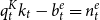 $q_t^K k_t - b_t^e = n_t^e$
and the nonnegativity constraint
 $W_{t+1}^e = \max \left \{ \omega _{t+1}^e \left (r_{t+1}^K + \left (1 - \delta _{t+1}^k \right )q_{t+1}^K \right ) k_t - R_t^F b_t^e,\: 0 \right \}$
, where
 $q_t^K$
represents the price of physical capital,
 $k_t$
is the physical capital held by the entrepreneurs,
 $r_{t+1}^K$
is the rental rate per efficiency unit of physical capital,
 $\delta _{t+1}^K$
is the time-varying depreciation rate of each efficiency unit of physical capital,
 $R_t^F$
is the contractual gross interest rate of the loans, and
 $\omega _{t+1}^e$
is an idiosyncratic shock to the efficiency units of physical capital which is independently and identically distributed across entrepreneurs. Entrepreneurs default on their loans whenever the gross returns on investment in physical capital undertaken in the previous period falls below the contractual repayments due to the bank. This occurs whenever the idiosyncratic shock
 $\omega _{t+1}^e$
exceeds the threshold
 \begin{equation} \overline {\omega }_{t+1}^e = \dfrac {R_t^F b_t^e}{R_{t+1}^Kq_{t}^K k_t}, \end{equation}
where
 $R_{t+1}^K = \left (r_{t+1}^K + \left (1 - \delta _{t+1}^k \right )q_{t+1}^K \right )/q_{t}^K$
.
3.3 Banks
There are two specialized banks in the model, denoted by
 $j \in \{ H, \:F\}$
. One type of bank,
 $H$
, provides credit to impatient households,
 $b_t^m$
, for investment in housing (mortgage loans) while the other type,
 $F$
, grants credit to entrepreneurs,
 $b_t^e$
, to their investment in physical capital (corporate loans). Banks use deposits,
 $d_t^j$
, and equity,
 $e_t^j$
, to finance themselves, which can be accumulated internally through retained earnings, and externally by raising equity from bankers.
Banks are subject to regulatory capital constraints and operate with limited liability. Specifically, banks face the capital constraint:
 \begin{equation} e_t^j \geq \phi _t^j b_t^j, \end{equation}
where
 $\phi _t^j$
is the bank’s capital ratio, and the constraint is always binding by definition. It is assumed that the bank’s capital ratio,
 $\phi _t^j = \Xi _t^j + \phi _{vol}^j$
, is composed of regulatory capital requirements,
 $\Xi _t^j$
, which may be constant or vary over time, and a time-invariant management buffer,
 $\overline {\phi }_{vol}^j$
, which reflects the portion of capital held above the minimum regulatory requirement. Unlike in reality, where banks often adjust their management buffers to accommodate regulatory changes, this model assumes that the buffer remains constant. As a result, any change in capital ratios directly translates into changes in lending capacity, which simplifies the model but may influence short-term dynamics. Nonetheless, capital requirements differ by loan type. In this model, mortgage loans carry a 50% risk weightFootnote
11
while corporate loans are assigned a 100% risk weight.
Bank equity is supplied by bankers and must match the total demand for equity from both mortgage-lending banks,
 $e_t^H$
, and corporate-lending banks,
 $e_t^F$
. Similarly, the deposits provided by patient households,
 $d_t$
, must equal the total demand for deposit funding from both types of banks,
 $d_t^H$
and
 $d_t^F$
. Consequently, the banking sector’s balance sheet constraint is given by:
 \begin{equation} n_t^b + d_t = b_t^e + b_t^m, \text{ with } n_t^b = e_t^H + e_t^F, \end{equation}
This constraint determines the total amount of credit banks can issue. Additionally, the sector-wide capital constraint can be expressed as:
 \begin{equation} n_t^b = \phi _t^F b_t^e + \phi _t^H b_t^m. \end{equation}
These two constraints play a key role in determining the transition dynamics of the banking sector. The effects on mortgage and corporate credit depend on how shocks impact bankers’ net worth and deposit availability, as well as the regulatory response. On the one hand, the capital requirement constraint tends to favor mortgage lending due to its lower risk weight. On the other hand, the balance sheet constraint directs resources toward the more profitable lending sector. The final allocation of resources between mortgage and corporate credit depends on the relative strength of these opposing forces.
Bank failure occurs when the observed return on its credit portfolio is lower than the obligations arising from the repayment of deposits and associated interest. Banks may default due to both idiosyncratic and aggregate shocks,
 $\omega _{t+1}^j$
, affecting the performance of their loan portfolios. In each period, the equity payoff for bank
 $j$
is determined by the difference between the returns on its loans and the repayments required on its deposits:
 \begin{equation} \pi _{t+1}^j = \max {\left[\omega _{t+1}^j \tilde {R}_{t+1}^j b_t^j - R_t^D d_t^j, \: 0\right]}, \end{equation}
where
 $b_t^j$
and
 $d_t^j$
represent the loans and deposits on bank
 $j$
balance sheet at time
 $t$
, respectively,
 $R_t^D$
is the gross interest rate paid on deposits taken at
 $t$
, and
 $\tilde {R}_t^j$
is the realized return on the portfolio of loans of class
 $j$
. Bank’s default occur due to fluctuations in the aggregate loan return
 $\tilde {R}_{t+1}^j$
, which is driven by firms’ and households’ default rates, as well as the bank-idiosyncratic shock,
 $\omega _{t+1}^j$
. The threshold level of
 $\omega _{t+1}^j$
below which the bank of type
 $j$
defaults is given by
 \begin{equation} \overline {\omega }_{t+1}^j = \left(1-\phi _t^j\right)R_t^D/\tilde {R}_{t+1}^j. \end{equation}
The threshold for bank’s default relates to the bank’s capital ratio,
 $\phi _t^j$
, and the spread between the realized gross loan return and the gross deposit rate,
 $R_t^d/\tilde {R}_t^j$
. An increase in the bank’s capital ratio positively impacts the default threshold, enhancing the bank’s ability to withstand adverse idiosyncratic shocks to its portfolio returns.
The aggregate default rate for the banking system,
 $PD_t^b$
, depends on the distribution of banks’ portfolios and the default probabilities of each bank type. It is given by:
 \begin{equation} PD_t^b = \dfrac {d_{t-1}^H F\left ( \overline {\omega }_t^H \right ) + d_{t-1}^F F\left ( \overline {\omega }_t^F \right )}{d_{t-1}^H + d_{t-1}^F}, \end{equation}
where
 $F\left ( \overline {\omega }_t^j \right )$
is the probability of default of a bank of class
 $j\in \left \{H,\: F \right \}$
.
3.4 Deposit insurance agency
Deposits are formally guaranteed by a deposit insurance agency (DIA), which covers the amount deposited and the corresponding interest. When necessary, the deposit guarantee system is financed through a fixed tax levied on households. However, recovering the fully insured amount is assumed to be costly, implying that deposits may still carry a risk premium reflecting the average bank’s default risk. This assumption accounts for depositors’ limited ability to monitor individual banks, making deposit risk premia dependent on the overall health of the banking sector. Within this framework, households incur a linear transaction cost,
 $\gamma$
, when recovering their funds, representing the time and effort involved in reclaiming deposits and interest following a bank failure. This cost establishes a direct link between the probability of bank default and bank funding costs, thereby creating a wedge between the deposit return rate and the risk-free rate:
 \begin{equation} \tilde {R}_t^D = R_{t-1}^D\left (1 - \gamma PD_t^b \right ), \end{equation}
which, in turn, raises the banking sector’s funding costs when default risk is high.
The aggregated losses to the DIA by failing
 $H$
and
 $F$
banks are given by
 \begin{equation} T_t = T_t^H + T_t^F = \underbrace {\left (\Omega _t^H(\bar {\omega }_t^H)\dfrac {\tilde {R}_{t}^H }{1-\phi _{t-1}^H}\dfrac {d^H_{t-1}}{d_{t-1}} + \Omega _t^F(\bar {\omega }_t^F)\dfrac {\tilde {R}_{t}^F }{1-\phi _{t-1}^F}\dfrac {d^F_{t-1}}{d_{t-1}}\right )}_{\Omega \left (\bar {\omega }_t^H,\bar {\omega }_t^F \right ) := \text{Average default loss per unit of bank debt}} d_{t-1}, \end{equation}
where
 $d_{t-1} = d_{t-1}^H + d_{t-1}^F$
is the aggregated deposits in the banking system, and
 $\Omega _t^H(\bar {\omega }_t^j) = \left [ \bar {\omega }_t^j - \Gamma ^j\left ( \bar {\omega }_t^j \right ) + \mu ^jG\left ( \bar {\omega }_t^j \right ) \right ]$
, for
 $j\in \left \{ H, \: F \right \}$
. Here,
 $\Gamma _t^j$
represents the expected fraction of defaulting bank’s assets that can be recovered, while
 $\mu ^j G^j\left ( \bar {\omega }_t^j \right )$
captures the total cost of bank default as a faction of total bank assets.
The deadweight default loss parameter,
 $\mu ^j$
, plays a critical role in shaping the relationship between capital regulation and banks’ internalization of the broader economic consequences of default. A lower value reduces the financial burden on households in funding the DIA.
This feature of the model creates incentives for banks to engage in excessive risk-taking practices, as it allows banks with a business model more focused on granting credit to higher-risk borrowers to implicitly benefit from a subsidy against banks with a more conservative lending profile. However, the model assumes that patient households do not know the risk profile of each bank, observing only the average risk of the sector.
3.5 Production sector and market clearing
Perfectly competitive firms producing the final good, new physical capital, and housing close the model in the production sector. In equilibrium, the total output in the economy is equal to the aggregate statistics of consumption, capital investment, housing investment, and wealth of bankers before dividends.
4. Calibration of the model
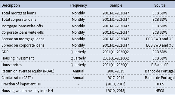
This section reports the results of the calibration of the 3D model for the Portuguese economy using quarterly data from 2001Q1 to 2020Q1.Footnote 12 The Common Equity Tier 1 capital ratio was calibrated based on a shorter time span, from 2017Q4 to 2019Q4. The main reason underlying this option is that the overall time span does not reflect the higher capitalization level of the Portuguese banking system in the periods ahead of the COVID-19 pandemic crisis.Footnote 13 The increased capitalization of banks resulted from stricter capital requirements put in place due to changes in capital regulation and the introduction of a macroprudential policy in the aftermath of the 2008 financial crisis and the sovereign debt crisis. Since the prudential measures we are assessing in this study are mainly related to capital buffers and requirements and given that the pandemic shock hit a more resilient banking system than the overall time span would suggest, we consider that the calibration of the model should reflect a better capitalized Portuguese banking system. The calibration strategy follows Lima et al. (Reference Lima, Maia and Pereira2023). We start with a first group of parameters that are preset according to the existing literature and conventions. Having fixed the first set of parameters, the calibration of the remaining ones takes into account the first and second moments of several macro-financial variables, that are used as targets to be matched by the model.
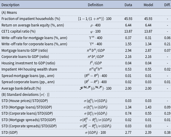
Table 1 reports the calibration targets, defined in terms of means and standard deviations, along with the values obtained from the model. Overall, the model matches the data well, since the theoretical first (mean) and second (volatility) moments computed from the model are equal, or very close, to the targeted empirical moments.
Calibration targets

Note: The Return on Average Bank Equity (ROAE) is based on positive values of the return on equity (ROE) and results from the time series average of the cross-sectional median ROE. Aggregate values for the banking sector consist of weighted averages across banks, with weights given by the share of each individual bank’s assets in total assets. HH stands for households, GDP for Gross Domestic Product, CET1 for Common Equity Tier 1, STD for standard deviation and Ann is short for annualized. The differences between the data and the model (Diff. column) are in absolute terms. Appendix A presents the details on data sources and frequencies.
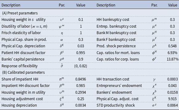
Table 2 reports the parameter values obtained from the calibration exercise. Panel (A) focuses on the parameters that were preset while panel (B) shows the parameters that were calibrated using the data targets from Table 1. The parameters in Panel (B) were jointly estimated by minimizing a loss function that assigns equal weight to the relative deviation between the empirical first and second moments and the corresponding (unconditional) moments generated by the model’s second-order approximation.
Parameters

Note: The disutility of labor is the same for patient and impatient households. HH stand for households, STD stands for standard deviation, Bank M stands for bank specialized in mortgage loans, Bank F stands for bank specialized in corporate loans.
 $s$
and
 $m$
stand for the households’ type, patient and impatient, respectively.
The labor disutility parameter,
 $\varphi ^{\varkappa }$
, is normalized to one for both households’ type, as it only affects the scale of the economy, while the weight of housing in patient households’ utility function is set at
 $0.1$
. The Frisch elasticity of labor,
 $\eta$
is normalized as well.Footnote
14
The share of capital in the production function,
 $\alpha$
, is set equal to
 $0.3$
, and the physical capital depreciation,
 $\delta ^K$
, is equal to
 $0.03$
. The capital ratios for mortgage and corporate loans,
 $\phi ^H$
and
 $\phi ^F$
, are set to
 $6.93\%$
and
 $13.87\%$
, respectively. These targets are associated with a risk weight of
 $100\%$
for corporate loans and of
 $50\%$
for mortgages (loans to households), as in Clerc et al. (Reference Clerc, Derviz, Mendicino, Moyen, Nikolov, Stracca, Suarez and Vardoulakis2015), to reflect the less stringent risk weights defined in the regulation for the former type of loans.Footnote
15
Despite the calibrated parameters in panel (B) of Table 2 being set simultaneously, some can be directly linked to one of the targets. The share of impatient households in total households,
 $n^m$
, matches the fraction of impatient households (proportion of indebted households). The bankers’ endowment,
 $\chi ^b$
, matches the median return on average equity (ROAE) for the O-SII group of the Portuguese banking sector. The households’ transaction cost (or bankruptcy cost parameter),
 $\gamma$
, is set in order to account for losses of
 $10\%$
of face value of deposits at failed banks. The housing weight in the utility of impatient households,
 $\upsilon ^m$
, is calibrated by targeting the share of housing held by the indebted households (value of the main residence of impatient households) in Portugal. The impatient households’ discount factor,
 $\beta ^m$
, and the new entrepreneurs’ endowment,
 $\chi ^e$
, are used to match the household mortgage to GDP and corporate loans to GDP ratios, respectively. The housing depreciation rate,
 $\delta ^H$
, is calibrated in order to match the ratio of housing investment to GDP. The standard deviations along with the housing and physical capital adjustment costs are used to match the remaining targets in panel (B) of Table 2.
5. The impact of the flexibility measure and the dividends pay-out restriction
In this section, we quantify the impact of the flexibility measure and the dividends pay-out restriction in an economic environment affected by the COVID-19 pandemic. We start by considering the joint effects of the flexibility measure and the dividends pay-out restriction, compared to a scenario where no-policy measures were implemented. It is reasonable to consider the two measures at the same time, since both were implemented with the same purpose of ensuring that banks keep supporting the economy. Given the sequential announcements of the prudential measures, we also consider the individual effects of the flexibility measure, the first measure to be announced.
It is important to stress that the results obtained do not factor in other policy measures that were also applied as a response to the pandemic, such as monetary and government policies adopted to mitigate the consequences of the pandemic, which are also transmitted through the banking sector.Footnote 16 Notwithstanding, the purpose of this exercise is to estimate the partial effect of the flexibility and the dividends pay-out restriction measures in the variables analyzed and not to predict the evolution of output and credit.
To simulate a shock with the magnitude and dynamics of the pandemic, we analyze the effects of a perturbation stemming from the supply side of the economy. Following Kollmann (Reference Kollmann2021), we focus on negative shocks to productivity to simulate a generalized adverse impact on the production of final goods and reproduce the GDP contraction observed in 2020. The use of the productivity shock is also justified by the conclusions of a study for the Portuguese economy (Banco de Portugal, 2020), suggesting that the GDP contraction was, to a large extent, determined by supply-side factors, and especially by the fall in global productivity.Footnote 17
As referred in such analysis, the productivity shock reflects the partial or total closure of firms and lockdown of certain economic activities at the global level and efficiency disruptions, affecting both labor and capital. Although the shocks considered operate through the supply side of the economy, they also have significant effects on the demand-side through the impact on income. This option has also been adopted in related literature that studies the economic consequences of the pandemic.Footnote 18 However, as the model does not take into account other measures implemented to mitigate the impact of the pandemic, the response of income to the shock in terms of magnitude may not be the same as the one observed in reality.
GDP dynamics, productivity, and dividends shocks.
Note: The empirical GDP in panel (A) (blue line) shows the deviation (in percentage) from the value observed in 2019Q4. The match in the model is set to the deviations of GDP from the equilibrium (steady state).

To simulate a supply disruption close to the size and dynamics observed in 2020 and 2021, we consider a series of productivity shocks that negatively affect output and set their magnitude to replicate the drops that occurred in the two lockdown periods starting in March 2020 and January 2021 (panel B of Figure 2). The persistence of the productivity shocks (see Table 2) was calibrated to follow (partially) the recovery observed before the second lockdown. Panel A of Figure 2 presents the observed dynamics of GDP from 2019Q4 to 2021Q4 and compares them with the ones obtained from the model, as a result of the productivity shocks that were considered in the simulation exercise. This comparison shows that the model replicates considerably well, not only the significant drop in GDP over the first 2020 quarters immediately after the onset of the pandemic crisis, but also the subsequent recovery as public policies helped mitigate its impact.
The banks’ response to the flexibility measure is simulated through a rule on the response of the capital ratio to deviations in total credit (the sum of loans granted to households and firms) from its steady-state level as:
 \begin{equation} \phi _t^j = \rho ^{\phi } \phi _{t-1}^j + \left (1 - \rho ^{\phi }\right ) \bar {\phi }^j + \underbrace {\bar {\vartheta } \left [ \log (b_t) - \log (\bar {b}) \right ]}_{\text{Flexibility measure}}, \end{equation}
where
 $\phi _t^j$
refers to the capital ratio of banks of type
 $j$
,
 $\rho ^{\phi }$
is the persistence of changes in banks’ capital ratio,
 $\bar {\phi }^j$
is banks of type
 $j$
’s capital ratio held in steady state,
 $\bar {\vartheta }$
sets the degree of response of the flexibility measure to total credit,
 $b_t$
, and
 $\bar {b}$
the respective steady-state level. The persistence of changes in banks’ capital ratio is set to
 $0.9$
, as we assume that any replenishment of capital buffers will not be required immediately but the decrease will not be permanent either. In this sense, the banks’ capital ratios are allowed to adjust to developments in the credit dynamics with some degree of rigidity.
The rule reproduces the aims of the flexibility measure, namely to ensure that banks continue to finance the economy. The response coefficient,
 $\bar {\vartheta }$
, was defined in such a way as to ensure that banks make full use of the flexibility provided by the measure throughout the projection period (2020Q1 to 2024Q4). The parameter is set to
 $0$
in the scenario where the policy measure is not active, and to
 $0.82$
—to generate a maximum 4 percentage points (p.p.) capital ratio reduction—when the policy measure is active. This calibration value assumes the full use of the Pillar 2 guidance and the combined buffer requirement by banks.Footnote
19
The dividends pay-out restriction is modeled as a shock on the share of bankers’ wealth transferred to patient households (owners of the banks). We introduce an auxiliary variable denoted as
 $\xi ^{\chi }$
into the equations governing the allocation of bankers’ wealth
 $\left (W_{t+1}^b\right )$
between distributing dividends
 $\left (c_{t+1}^b\right )$
and retaining earnings
 $\left (n_{t+1}^b\right )$
:
 \begin{align}&\quad c_{t+1}^b = \left(\chi ^b - \xi _{t+1}^{\chi }\right)W_{t+1}^b \end{align}
 \begin{align}& n_{t+1}^b = \left(1 - \left(\chi ^b - \xi _{t+1}^{\chi }\right)\right)W_{t+1}^b \end{align}
where
 $\xi ^{\chi }$
is defined by:
 \begin{equation} \xi _{t+1}^{\chi } = \xi _{t}^{\chi } + \epsilon _t^{\chi } - \epsilon _{t-6}^{\chi }. \end{equation}
In line with the ECB/SSM Recommendations, the suspension of dividends pay-out is implemented in the model in the second quarter of 2020 and remains active until the third quarter of 2021.Footnote
20
In terms of the model, transfers from banks to households in the form of dividends are eliminated from the
 $2^{{\textrm nd}}$
quarter to the
 $7^{{\textrm th}}$
quarter of our simulation, and additional profitability is used to provide credit to the economy (panel C of Figure 2).Footnote
21
,
Footnote
22
This is achieved by setting the magnitude of the shock
 $\epsilon _t^{\chi }$
to be equal to the value of bankers’ endowment
 $\chi ^b$
.
Three scenarios are considered in the following exercises, covered in Sections 5.1 and 5.2: i) a baseline scenario in which both the flexibility and the dividends pay-out restriction measures are in force; ii) a no-policy scenario, in which we assume that there were any policy measure implemented; and iii) a counterfactual scenario, in which we assume that only the flexibility measure is applied. In the counterfactual scenario, we also assume that banks fully utilize the flexibility measure in the active policy scenario. A comparison of results between these scenarios allows us to assess the joint and individual effectiveness of the measures.
5.1 The flexibility measure and the dividends pay-out restriction
This subsection presents the results of a simulation exercise of the joint effects from the combined implementation of the flexibility measure and the dividends pay-out restriction, compared to the no-policy scenario.
In the no-policy scenario, where the measures are assumed not to be available, the results obtained from the shocks applied in the model simulate an output path characterized by a sharp fall in the second quarter of 2020 followed by a gradual recovery, which is temporarily halted in the first quarter of 2021 as a result of new lockdown measures. Thereafter, a gradual recovery toward steady-state values is simulated (see Figure B3 in Appendix). The shock transmission mechanism initially leads to a decline in spending and production, which brings down the relative price between housing and physical capital. In the labor market, working hours and wages decline. The default of firms and households increases, which results in an increase in bank interest rates and a decrease in credit. The increase in banks’ default induces a higher cost of deposits, which in turn is passed through to households and firms via increased spreads in credit operations that further increase bank interest rates.Footnote 23 These effects spill over to the economy in the following periods, as they have a negative impact on investment, thereby amplifying the initial impact of the shocks. The recovery process is slow, in particular for credit. The increase in banks’ default induces additional costs on deposit insurance, supported by households, while overall deterioration of wealth reduces patient households’ income from owning banks and firms. This set of occurrences frames a strong, and moderately persistent, contraction in consumption—which after 5 years is still below its steady-state level.
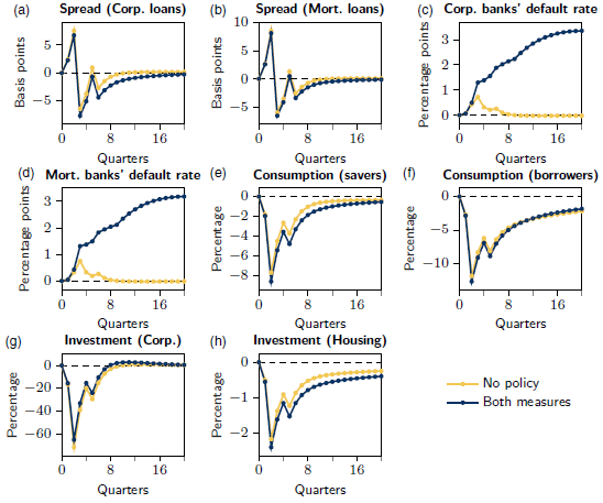
In the baseline scenario, banks use the flexibility measure and refrain from distributing part of their profits in the form of dividends. The dividends pay-out restriction allows banks to increase their management capital buffers, becoming more resilient to adverse shocks (Figure 3). Strengthening capital ratios in this manner allows banks to have additional resources that are at the outset fully used to finance the economy, which contributes positively to dampening the contraction in credit to households and firms that follows the shock. In the first three years following the implementation of the policy measures, the dividends pay-out restriction cumulatively reduces the decline in credit by 9%. When combined with the impact of the flexibility measure, this results in a total credit injection that is 48.4% higher than in the no-policy scenario. In other words, the two policy measures together halve the decline in credit.
Impact of the measures to shocks simulating a contraction in GDP.
Note: The impact is measured as the difference between the baseline scenario and the no-policy scenario.

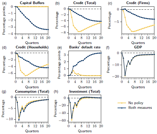
Banks apply a higher spread to corporate credit than household credit as, in our calibration, corporate loans are associated with a higher risk weight.Footnote 24 This characteristic is reflected in the different magnitude of the impact of shocks (see Figure B1 in Appendix). This leads to the measures having a greater impact on smoothing the decline in corporate loans than in mortgage loans, that is, the reduction in the cost of financing for firms is greater than the reduction in the cost of financing for households.
The smaller contraction in corporate loans is passed on to the economy through higher investment in physical capital, mitigating the effects of shocks and actively contributing to the faster recovery of GDP against the no-policy scenario. Over a three-year period, the dividends pay-out restriction prevents a 1.4% GDP loss. Combined with the impact of the flexibility measure, this adds up to a total GDP preservation of 2.7%.
The results of this simulation exercise highlight the complementary effect of the dividends pay-out restriction on mitigating the spillover of risk events to the economy. The effects of the two measures analyzed in this paper are transmitted to the economy through the credit channel resulting in a faster economic recovery.
5.2 The flexibility measure only
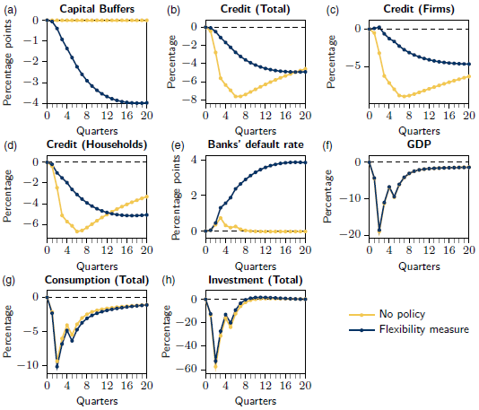
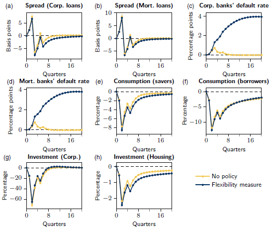
In the previous subsection, results indicate that there are benefits to financial stability from combining the flexibility measure with the dividends pay-out restriction policy. Now, we question what would be the effects to financial stability if only the flexibility measure was in place. This assumption could be explained by, to a large extent, banks not being keen to comply with the dividends pay-out restriction measure, for example, or by the decision of policy authorities to only apply the flexibility measure. A comparison of the results (Figure 4) allows us to assess the measure’s effectiveness in promoting the financial intermediation function of the banking system and in stabilizing the economy compared to the other two scenarios.
In the counterfactual scenario, banks make use of the flexibility they are provided with, using the capital buffers in response to deviations of total credit from its initial preshock value. Compared to the no-policy scenario, the flexibility measure mitigates the reduction in credit to households and firms. The effect is more pronounced in corporate loans, as this segment has higher risk weights. The credit smoothing effect is mainly reflected in investment, particularly in investment in physical capital by firms whose decline is mitigated in the first quarters. The improvement in the capacity to finance the economy dampens the fall in GDP over the first 13 quarters, although to a lesser extent than in investment. After that, due to a lower recovery rate, the effect of the flexibility measure becomes negative. Nonetheless, the net effect of the flexibility measure on GDP is still positive and although the effects on GDP of a reduction in capital ratios are relatively subdued, given that the shock is exogenous to the banking system, these results as well as those related to credit smoothing are in line with the aim of the capital requirements. Such regulation should in fact improve ex-ante the resilience of banks to prevent the propagation of shocks in the financial sector to the real economy, and help to mitigate adverse outcomes in the financial system from stress events with outside origination, avoiding amplification effects. In the first three years, the flexibility measure cumulatively injects 39.4% more credit compared to the no-policy scenario, helping to avert a 1.2% GDP loss.
Impact of the flexibility measure.
Note: The impact is measured as the difference between the counterfactual scenario and the no-policy scenario.

The higher leverage of banks due to the flexibility measure is perceived as an increased risk in the banking system which is translated into higher banks’ default rates. This increase in the probability of banks’ default imposes a higher cost on households with deposit insurance, which motivates a greater reduction in consumption. Consequently, the flexibility measure moderately intensifies the contraction in consumption that was registered under the no-policy scenario.
The introduction of capital requirements, together with the possibility of using part of them in a situation of stress in the financial system, reduces the materialization of risks from spreading into the economy, as they provide the banking system with greater capacity to absorb losses. However, the effectiveness in containing the transmission of disruptions that arise first in the economy and only then in the banking system is lower (see also Lima et al. (Reference Lima, Maia and Pereira2023)). It may thus be necessary, depending on the magnitude of the shock, to implement other support measures that complement each other and allow the economy to recover from the pandemic crisis.
For consumption, the impact of the two combined measures does not differ much from the case where we only consider the flexibility measure, meaning that the dividends pay-out restriction barely affects the consumption decisions of agents. The slightly worse combined effect of the measures on consumption between the third and the ninth quarter is motivated by a reduction in households’ income due to the dividends pay-out restriction. After this period, the combined effect becomes positive and contributes to a slightly faster convergence of consumption to its prepandemic level. The dividends pay-out restriction has also the additional effect of reducing the need for banks to use the flexibility measure to mitigate the effects of the shock and keep financing the economy. This outcome reflects how the two measures complement each other and shows that by restricting dividends pay-out, banks have to make a smaller effort to return to the level of capitalization that existed before the shock materialized. Although the flexibility measure was only partially used, its relative impact on all variables is decisive. The banking sector plays an active role in the economic recovery contributing to a less pronounced contraction in corporate investment compared to the no-policy scenario, which has an impact on the performance of economic activity.
To sum up, results indicate that a prudential measure that introduces flexibility in banks’ capital use in situations of stress is effective in promoting the financing of the economy, even if it is the sole measure in place. By being able to make full use of this flexibility, banks mitigate the transmission effect of the shock to credit granted to both firms and households. This measure is particularly beneficial for corporate loans, resulting in more favorable dynamics for corporate investment.
6. The replenishment of capital buffers
As shown in the previous section, there are benefits for the economy from the combined use of the supervisory measures that were implemented at the outset of the pandemic crisis. As the peak of the pandemic crisis is overcome and policymakers start to plan the exit strategy of policy measures, considering potential procyclical effects on lending driven by the replenishment of capital buffers becomes fundamental. In this section, we follow a conceptual approach to analyze this question. We consider different time spans for the replenishment of capital buffers and assess their implications for financial stability and economic activity. We assume that the replenishment paths are known to the financial system, given the decisions communicated by the supervisory authorities in due time. We focus on (i) potential costs and benefits of a smoother versus a more abrupt transition and (ii) potential costs of different paces in each transition period. Thus, this section flags the importance for the financial system to trigger an efficient adjustment to these buffers.
In this exercise, and differently from the previous section’s exercises, we abstract from a specific COVID-19 pandemic shock as we simulate an economy with released capital buffers in equilibrium that need to be replenished. Nevertheless, to be consistent with the magnitude of the flexibility measure discussed before, we consider replenishment paths leading to a 4 p.p. permanent change in capital buffers.Footnote 25 During the replenishment period banks are not subject to the dividends pay-out restriction. The macroprudential authority requires banks to raise capital, which gives rise to a new economic equilibrium once the higher level of capital buffers is achieved.Footnote 26
In the model, there are two transmission channels of capital buffers. On the one hand, a permanent increase in capital buffers driving the economy to a new steady state enhances the banking sector’s resilience by reducing bank failure probabilities and associated social welfare costs. Decreasing bank failure risk leads to a fall in deposit interest rates, which, ceteris paribus, reduces the average cost of bank financing and lending interest rates, besides stimulating credit. For this reason, an increase in capital buffers can lead to long-run increases in investment, consumption, output, and social welfare. On the other hand, increasing capital buffers can also trigger deleveraging and higher funding costs for borrowers, specifically when transitioning to higher levels. Strengthening capital buffers increases the demand for capital, making the average cost of bank funding more expensive. The higher average bank funding cost is transferred to borrowers through higher interest rates, causing a drop in lending. The final impact of an increase in capital buffers on interest rates and loans will thus depend on the relative magnitude of these two effects.
In the analysis, we put forward several transition scenarios. In the first scenario, capital buffers rise sharply. In the second scenario, we set four transition periods to assess whether they can mitigate the effects of a potential procyclical role for banks. The shorter and longer transition periods last 4 and 16 quarters, respectively. The choice of a one-year replenishment period as a minimum is coherent with CCyB regulation, which allows banks to comply with the buffer rate within one year. The maximum four-year period builds on the regulatory framework for the capital conservation buffer and the O-SIIs (Other Systemically Important Institutions) buffer.
In addition to the length of the adjustment period, it is also relevant to examine the pace at which capital buffers increase. Authorities have been favoring linear path regimes over time. In the following sections, we present the results of a linear regime and a nonlinear regime, in which we assume a faster pace of convergence to higher levels of capital buffers.
6.1 Linear path regime
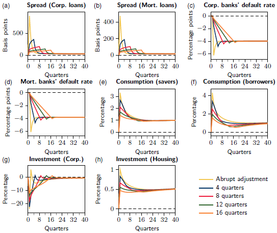
The impulse response functions (thereafter IRFs) for an abrupt increase in capital buffers and for the linear replenishment paths are presented in Figure 5. Before analyzing the results for the different transition periods, we focus on the responses to an abrupt increase of 4 p.p. in capital buffers, which represent a relevant reference point for the following considerations.
IRFs of capital buffers’ replenishment (linear path regime).
Note: Impulse responses from a
 $4$
p.p. capital buffers’ replenishment. Deviations from the initial steady state.

An abrupt adjustment in capital buffers has positive effects by reducing the probability of bank failure quickly, increasing the banking system resilience. However, it also induces high bank financing costs translating into higher spreads for borrowers.Footnote 27 The significant increase in interest rates is associated with a considerable reduction in total credit granted to the economy, in particular, in loans to businesses, as they bear the brunt of higher interest rates. This behavior also stems from the risk weights for housing credit being smaller than for corporate loans. These effects spill over to the economy: on the one hand, a greater resilience of the banking system has positive effects on household income, consumption and output, while, on the other hand, the sharp fall in credit triggers a significant drop in investment.Footnote 28 The effects of an abrupt increase in capital buffers unwind after a few quarters, and the economy quickly converges to a new equilibrium, where total credit and output are higher, and bank resilience is strengthened.
Results indicate that the permanent increase in capital buffers considered in the model, even if abrupt, has beneficial effects on financial stability and economic activity in the long run, but may trigger severe disruptions in banks’ financial intermediation function throughout the process of convergence to the new equilibrium. Therefore, we now consider longer transition periods in order to assess whether they allow the mitigation of the procyclical response of the banking system without significantly compromising the benefits arising from replenishing capital buffers.
In the linear replenishment paths, we observe how in general, predictable timing and speed of transition allow banks to anticipate the necessary adjustment in each period, smoothing the rise in spreads and the fall in lending, compared with an abrupt increase. The smoothing effect on corporate loans also leads to a less sharp decline in business investment. The longer the transition period, the more significant the smoothing effect. However, the fall in business investment is still more significant than the increase in residential investment, which benefits from house purchases by households that are not dependent on bank financing. This evidence determines that overall investment remains below—although closer to—its initial value throughout the convergence process to the new equilibrium. Longer transitions also mitigate the positive effects on the banking system resilience, if compared with an abrupt adjustment. Longer transition periods reduce the bank failure rate, but to a lesser extent than an abrupt adjustment. Moreover, they postpone the convergence of this variable to the new equilibrium.
The less favorable behavior of the bank failure rate has macroeconomic impacts due to a lower increase in consumption, as households must bear higher costs associated with deposit guarantees, and, consequently, in GDP. The speed of adjustment towards equilibrium is also slower. The choice of the transition path thus entails macroprudential policy trade-offs. The model favors shorter transition horizons if the macroprudential policy’s purpose is mainly to strengthen the banking system resilience. If the focus is mainly on maintaining the flow of credit to the economy, then longer time horizons are preferable.
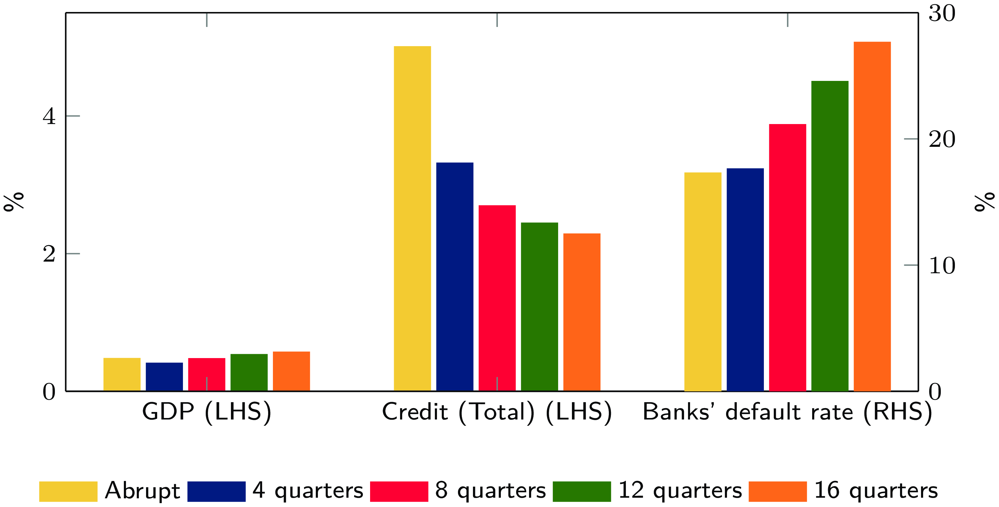
In addition to the previous analysis, we compute volatility metrics for the variables considered relevant for macroprudential policy: bank failure rate, credit, and output. We calculate the volatility associated with each of the three variables on the basis of the IRFs arising from the abrupt adjustment and the four transition periods adopted considering a linear pace of capital buffer accumulation (Figure 6).
The analysis indicates that longer transition periods lead to a significant reduction in overall credit volatility, which can be considered a benefit associated with longer time horizons. On the contrary, GDP and bank failure rate take more time to converge to the new equilibrium when the replenishment period is longer. Thus, as the transition period is extended, the volatility of GDP and bank failure rate increases. This result can be perceived as a cost associated with longer transition periods.
Volatility measures for the capital buffers’ replenishment paths (linear path regime).
Note: The volatility for each variable is obtained by calculating the standard deviation of the IRFs from their final steady-state values.

6.2 Nonlinear path regime
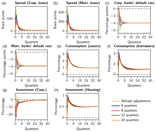
This section examines the effects of implementing nonlinear replenishment paths. In particular, we consider a decreasing rate for the required replenishment of the capital buffers (Figure 7).Footnote 29 This scheme may prove more effective in booming periods in the business and/or credit cycle, where higher buffer requirements can be more easily met by banks, by retaining profits and/or issuing capital, without disrupting lending activity.
The main conclusion drawn from the previous exercise still holds. Considering longer transition periods—compared to an abrupt adjustment—mitigates the costs of increasing capital buffers, yet it also curtails the development of a more resilient banking system. In a nonlinear path regime of capital buffer accumulation, the differences in the responses of the variables for each transition period are evident for the shorter horizons but fade out as horizons lengthen.
IRFs of capital buffers’ replenishment (nonlinear path regime).
Note: Impulse responses from a
 $4$
p.p. capital buffers’ replenishment. Deviations from the initial steady state.

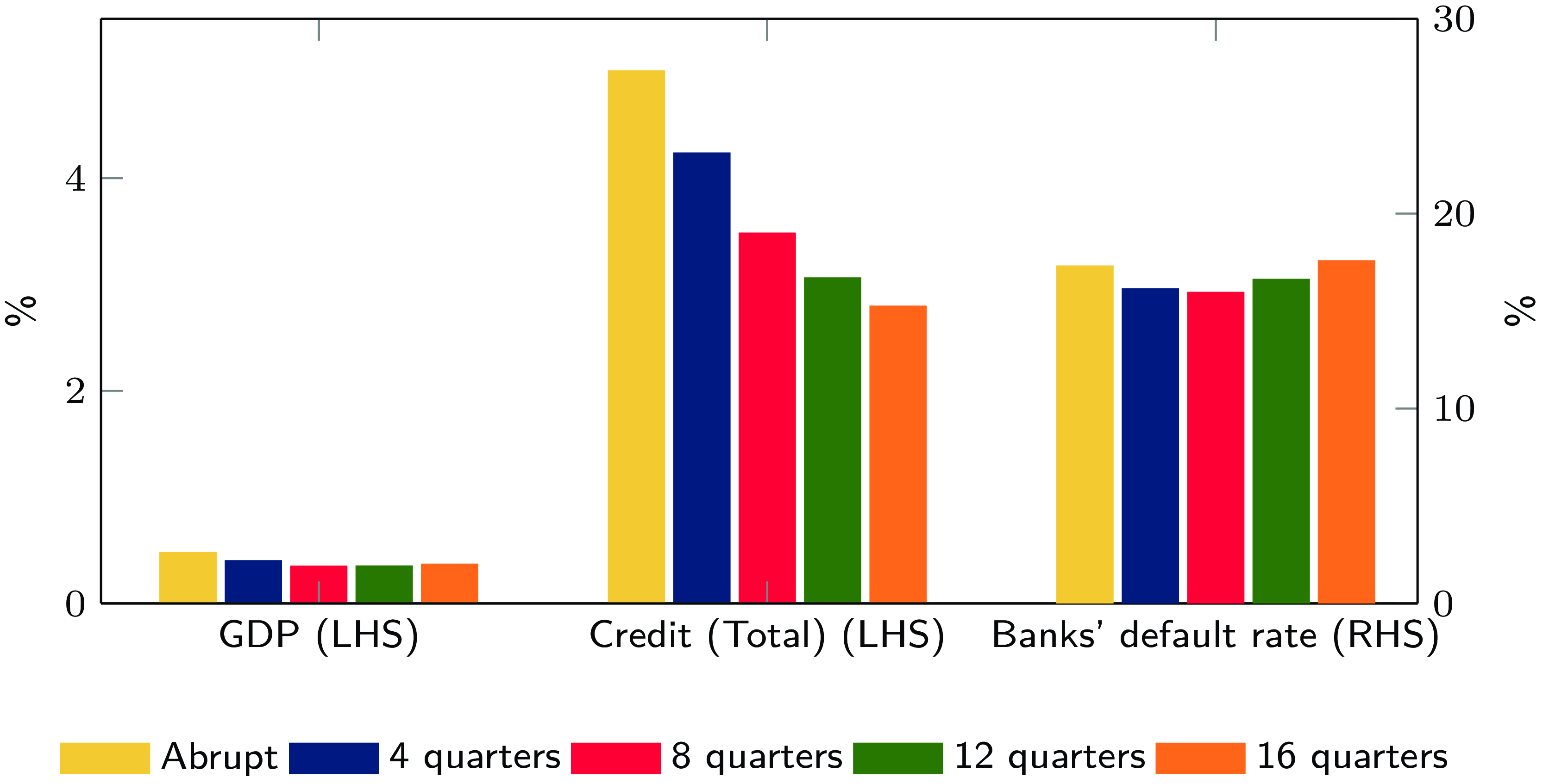
Compared with the results of the linear path regime for the corresponding transition periods, the nonlinear path regime leads to higher credit volatility (Figure 8). On the contrary, the volatility of output and bank failure rate are lower in the nonlinear path regime. Moreover, comparing the two path regimes, we can observe that changing the replenishment periods has a smaller effect on bank failure rate in the nonlinear regime. Additional simulation exercises for nonlinear path regimes suggest no significant benefits from choosing transition periods longer than 16 quarters.Footnote 30
Volatility measures for the capital buffers’ replenishment paths (nonlinear path regime).
Note: The volatility for each variable is obtained by calculating the standard deviation of the IRFs from their final steady-state value.

7. Sensitivity analysis
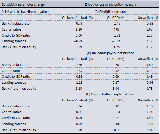
This section examines how the calibration presented in Section 4 influences the magnitude of our results.Footnote 31 Given the model’s large number of parameters, we focus on varying a few key steady-state calibration values while keeping the others fixed: banks’ default, capital ratios, credit-to-GDP ratios, lending spreads, and banks’ return on equity (ROE). Appendix D presents the results and methodological details of the sensitivity analysis.
Since our results demonstrated that the flexibility measure and the dividends pay-out restriction affect the economy through distinct channels—and thus differently—we isolate their individual impacts in the sensitivity analysis. The results for the flexibility measure suggest that banks’ default and capital ratio steady-state values are crucial in determining the policy effectiveness on the resilience of the banking system, measured by the magnitude of the reduction in banks’ default. Meanwhile, credit-to-GDP ratios, lending spreads, and banks’ ROE also play a significant role in shaping the effectiveness on GDP, measured by the magnitude of its increase.
The effectiveness of the dividends pay-out restriction on banking system resilience benefits primarily from higher steady-state bank profitability, while is hindered by high credit-to-GDP ratios and lending spreads. A 1% increase in the steady-state capital ratio makes the dividends pay-out restriction 0.52% more effective in sustaining economic activity, reinforcing its mitigating role in credit contraction, as discussed in Section 5.1.
Banks’ default and capital ratio steady-state values are the key drivers of capital buffer replenishment effectiveness, with the policy being generally more effective when banks face higher risk in equilibrium (i.e., a high default rate and low capital ratios). In contrast, the steady-state credit-to-GDP ratio primarily influences the impact on GDP, as more indebted economies benefit more from the replenishment.
The sensitivity analysis also sheds light on the welfare implications of the measures we have analyzed. This is particularly relevant for the flexibility measure and the dividends pay-out restriction because, despite supporting banking system resilience and output, they tend to reduce consumption—especially in the short run—resulting in limited or even negative welfare effects.
Higher steady-state levels of capital ratios, lending spreads, and credit-to-GDP ratios generally increase the effectiveness of the flexibility measure in welfare terms. In contrast, higher steady-state lending spreads weaken the welfare performance of the dividend restriction, even though the impact remains positive when the two measures are implemented jointly. Our findings indicate that these measures may be more welfare-enhancing when implemented in financially weaker systems, where the risk of instability is higher and the credit channel is more impaired. Conversely, in sounder financial environments, such as the one represented by our baseline calibration, these tools might stabilize the system at the cost of household welfare. This underlines the importance of tailoring policy interventions to the underlying source and intensity of financial stress.
8. Conclusions
Among other policies, European prudential authorities adopted the flexibility measure and the dividends pay-out restriction to mitigate the detrimental effects of the COVID-19 pandemic to the economic and financial situation. These measures prevented the potential deleveraging of banks and supported the financing of the real economy at a time of severe supply and demand contraction. As the most disruptive crisis phase is over, rebuilding capital buffers becomes a fundamental task for policymakers who plan the exit strategy of policy measures.
Our work seeks to evaluate the economic and financial impacts of the flexibility measure and the dividends pay-out restriction and comprehend the implications for financial stability and economic activity of different periods and paces for the replenishment of capital buffers in the aftermath of the measures’ withdrawal. The assessment of the outcomes of these policy measures on the financial system can contribute to a more effective use of the macroprudential policy tools that policymakers can use to promote financial stability.
To achieve our objective, we adopt a DSGE model calibrated for the Portuguese economy where banks, impatient households, and entrepreneurs can default. In the model, micro- and macro-prudential capital regulation contributes to dampening the financial distortions.
Our results suggest that the flexibility measure is effective in promoting the flow of credit in the economy. The transmission of the COVID-19 pandemic shock to households and firms credit is restrained, especially for corporate loans. The credit smoothing effect translates into a smaller decrease of investment, particularly in physical capital. The flexibility measure has a positive net impact on GDP, reducing its fall as the COVID-19 pandemic materializes.
The joint use of the flexibility measure and the dividends pay-out restriction strengthens the favorable aforementioned effects. By preventing the distribution of part of the profits in the form of dividends, banks raise their management capital buffers, improving resilience to adverse shocks, and use all additional resources to finance the economy. The measure thus contributes to mitigate the reduction in credit to households and firms caused by the COVID-19 pandemic shock. In addition to complementing the flexibility measure, the dividends pay-out restriction has the benefit of easing the effort of the banking system—and therefore the impact on the economy—to subsequently rebuild capital buffers. This measure reduces the magnitude of the capital buffers drop that banks generate when applying the flexibility measure, which will constitute the extent of the replenishment.
Results for the replenishment of capital buffers show that a permanent increase in capital buffers is beneficial for financial stability and economic activity in the long run, but may be detrimental to the financial and economic system throughout the process of convergence to the new equilibrium depending on the transition periods. In general, shorter and more abrupt transitions are more effective at reinforcing banks’ resilience, and longer transitions are more appropriate for ensuring a higher flow of credit to the economy. We conclude that the choice of the most suitable transition path entails trade-offs, and depends on the primary and contingent objectives of policymakers. Adopting linear or nonlinear path regimes does not influence this main result, even if the longer transition paths seem to have a small additional impact with respect to the shorter transition paths in the nonlinear regime.
Acknowledgements
We thank Inês Drumond, Ana Cristina Leal, José R. Maria, Ana Pereira, Martín Saldías, Fátima Silva, and the participants of the 6th Annual Workshop of ESCB Cluster 3 for the helpful comments. We acknowledge the work and the sharing of codes of the ECB Task Force on Operationalizing Macroprudential Research. The views expressed in this article are those of the authors and do not necessarily reflect the views of Banco de Portugal or the Eurosystem. Any errors and mistakes are ours. The paper reconciles previous work developed in three editions of the Banco de Portugal Financial Stability Report: December 2020, June 2021, and December 2021.
Competing interests
The authors declare none.
Appendix A. The data
Data used in the calibration exercise

Notes: SWD stands for Statistical Data Warehouse, OC stands for own calculations, SP stands for Statistics Portugal, HFCS stands for Household Finance and Consumption Survey, ECB stands for European Central Bank, and BIS stands for Bank for International Settlements.
Appendix B. The impact of the flexibility measure and the dividends pay-out restriction: Impulse response functions (IRFs)
B.1. The flexibility measure and the dividends pay-out restriction
IRF for the baseline and no-policy scenarios to the shocks simulating a contraction in GDP.

IRF for the baseline and no-policy scenarios to the shocks simulating a contraction in GDP (additional variables).

B.2. The flexibility measure
IRF for the counterfactual and no-policy scenarios to the shocks simulating a contraction in GDP.

IRF for the counterfactual and no-policy scenarios to the shocks simulating a contraction in GDP (additional variables).

Appendix C. The replenishment of capital buffers: additional impulse response functions (IRFs)
C.1. Linear path regime
Additional IRFs of capital buffers’ replenishment (linear path regime).
Note: Impulse responses from a
 $4$
p.p. capital buffers’ replenishment. Deviations from the initial steady state.

C.2. Nonlinear path regime
Additional IRFs of capital buffers’ replenishment (nonlinear path regime).
Note: Impulse responses from a
 $4$
p.p. capital buffers’ replenishment. Deviations from the initial steady state.

Appendix D. Sensitivity analysis
Sensitivity analysis on key steady-state values and parameters of the model

Notes: “s.s.” stands for steady state. The analysis is performed by modifying the relevant target in Table 1 while keeping the others unchanged. The ranges used for each steady-state value we modified are as follows: for (average) banks’ default rate
 $[1.6\%, 7.5\%]$
, for (average) capital ratios
 $[9.86\%, 13.86\%]$
, for (average) credit-to-GDP ratio
 $[1.85, 2.80]$
, for (average) lending spreads
 $[0.011 \text{ p.p. (ann.)}, 0.025 \text{ p.p. (ann)}]$
, for (average) banks’ return on equity
 $[3.22\% \text{ (ann.)}, 25.76\% \text{ (ann.)}]$
. As a consequence, some steady-state relationships change slightly during the sensitivity analysis. Still, we have verified that such changes are negligible and do not affect the overall message of the results. In A. and B., for banks’ default, effectiveness measures the cumulative reduction in default in the baseline scenario compared to the no-policy scenario. For GDP and welfare, effectiveness measures the cumulative increase in GDP and welfare in the baseline scenario compared to the no-policy scenario. In C., for banks’ default, effectiveness measures the reduction in default in the steady state after capital buffers are replenished compared to before replenishment. For GDP and welfare, effectiveness measures the increase in GDP and welfare in the steady state after capital buffers are replenished compared to before replenishment. The impact on effectiveness of a 1% increase of each parameter compared to its baseline steady-state value is captured by
 $\beta _1$
in the log-log regression model
 $log(y)=\beta _0 + \beta _1 log(x)$
, where
 $x$
is the vector of parameter values analyzed in the sensitivity analysis and
 $y$
is the corresponding vector of effectiveness values. Welfare is computed as:
 $\tilde {V}_t \equiv \zeta V_{s,t} + (1 - \zeta ) V_{m,t}$
, where
 $V_{\varkappa ,t} = U(c_{\varkappa ,t}, h_{\varkappa ,t}, l_{\varkappa ,t}) + (\beta _{\varkappa }) \mathbb{E}_t V_{\varkappa ,t+1}$
and
 $\varkappa ={s,m}$
. This specification follows Mendicino et al. (Reference Mendicino, Nikolov, Suarez and Supera2018). We choose the welfare weights as the consumption shares of each household type in steady state:
 $\zeta = {c^s}/{(c^s + c^m)}$
and
 $1 - \zeta = {c^m}/{(c^s + c^m)}$
.