1 Introduction
There are some interesting phenomena in the context of water waves associated with a long but finite array of circular cylinders. Near trapping of waves by a finite periodic straight-line array of cylinders, closely related pure trapping of waves and Rayleigh–Bloch waves for an infinite array have been studied extensively.
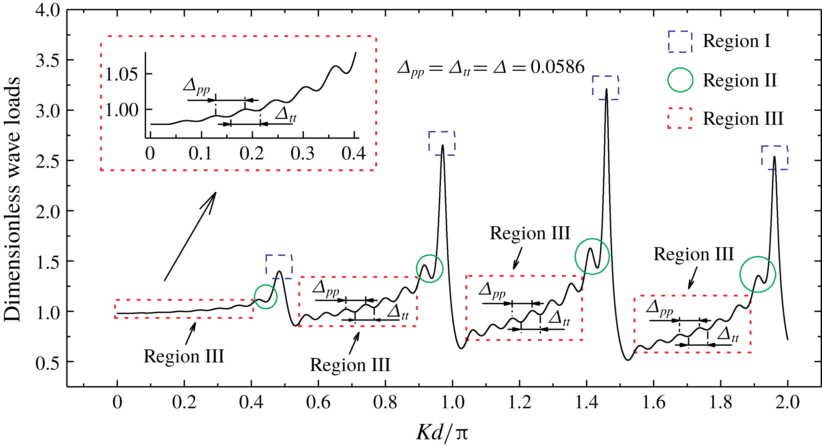
Regions I, II and III for the curve of the variation of magnitude of wave load acting on the middle cylinder of an array consisting of 17 cylinders, with diameter-to-spacing ratio
 $a/d=1/6$
. The incident waves propagate parallel to the array (
 $\unicode[STIX]{x1D6FD}=0$
).

Motivated by the work of Maniar & Newman (Reference Maniar and Newman1997), we computed the wave loads (i.e. the integrals of pressure over the wetted surface) on any cylinder in many arrays of bottom-mounted circular cylinders in the context of linear water waves. Each array consists of
 $N$
identical cylinders spaced equally along the array. The total number of cylinders and the diameter-to-spacing ratio are different for each array. In addition to the cases of number of cylinders
 $N=9$
,
 $100$
and
 $101$
in Maniar & Newman (Reference Maniar and Newman1997), we investigated many other cases such as
 $N=11,21,31,51$
and 301 for diameter-to-spacing ratios
 $a/d=1/2$
,
 $1/4,1/6$
and
 $1/8$
, where
 $2a$
is the cylinder diameter and
 $2d$
the spacing between the axes of adjacent cylinders. For a wave load acting on any cylinder in these arrays along the array, variations in the magnitude of the load with the non-dimensional wavenumber
 $Kd/\unicode[STIX]{x03C0}$
(
 $K$
is the wavenumber) were observed to have the following distinct features in common. (1) Several towering spikes occur when the wavenumber
 $Kd/\unicode[STIX]{x03C0}$
is slightly lower than the integer multiple of
 $1/2$
. In the present study, the region containing the spikes is termed Region I. (2) A sequence of secondary peaks and intermediate troughs occur at wavenumbers slightly lower than the wavenumbers corresponding to the spikes. These secondary peaks are lower than the spikes. The region containing the secondary peaks and troughs is termed Region II in the present study. (3) Apart from Regions I and II, the remainder of the load–wavenumber curve is termed Region III in the present study. Most parts of the curve belong to this region. In Region III, fluctuation of the load–wavenumber curve is very regular. A schematic diagram of Regions I, II and III is shown in figure 1. This figure shows the variation in magnitude of the load with the non-dimensional wavenumber for the middle cylinder of an array with
 $N=17$
,
 $a/d=1/6$
, in head waves (i.e. incidence angle
 $\unicode[STIX]{x1D6FD}=0$
). The magnitude of load is normalized by the corresponding result for a single isolated cylinder. Many studies of the behaviours and the physical meanings of Regions I and II have been published. However, there are few studies of Region III. We investigate the fluctuation characteristics of Region III in the following sections. As shown in figure 1, for the load–wavenumber curve, the horizontal spacing between two adjacent local maximum points
 $\unicode[STIX]{x1D6E5}_{pp}$
and that between two adjacent local minimum points
 $\unicode[STIX]{x1D6E5}_{tt}$
in Region III are equal and constant. For this example,
 $\unicode[STIX]{x1D6E5}_{pp}=\unicode[STIX]{x1D6E5}_{tt}$
, and they are almost always 0.0586. Let
 $\unicode[STIX]{x1D6E5}~(=\unicode[STIX]{x1D6E5}_{pp}=\unicode[STIX]{x1D6E5}_{tt})$
be the fluctuation spacing. It is observed that for any straight-line array of cylinders,
 $\unicode[STIX]{x1D6E5}$
remains unchanged in Region III (i.e.
 $\unicode[STIX]{x1D6E5}$
is independent of
 $Kd/\unicode[STIX]{x03C0}$
) and depends only on
 $N$
,
 $k$
and
 $\unicode[STIX]{x1D6FD}$
. Here
 $k$
is the identification number of a cylinder in the array that indicates cylinder position. In the present study, we find that the fluctuations in Region III are regular and propose formulae for determining the fluctuation spacing in this region.
Maniar & Newman (Reference Maniar and Newman1997) studied the near-trapping of waves in a finite periodic straight-line array of cylinders. They associated the wavenumber at which an unusually large load occurs with the wavenumber corresponding to the homogeneous solutions (trapped waves) for an infinite array of cylinders or a cylinder confined between two parallel walls. The trapped modes near a vertical cylinder standing between the walls of a channel and the proof of existence have been investigated by Callan, Linton & Evans (Reference Callan, Linton and Evans1991), Linton & Evans (Reference Linton and Evans1992a ), Evans, Levitin & Vassiliev (Reference Evans, Levitin and Vassiliev1994) and Newman (Reference Newman2017). The unusually large load referred to as towering spikes in Region I in the present study can be explained by the aforementioned studies.
More general problems include the trapped modes near a finite number of cylinders spaced periodically across a channel and Rayleigh–Bloch waves along an infinite periodic array of cylinders. Rayleigh–Bloch waves are surface waves which propagate along the array and decay exponentially with distance from the array. Porter & Evans (Reference Porter and Evans1999), based on using an appropriate Green function, studied Rayleigh–Bloch waves travelling along an infinite array of identical bottom-mounted cylinders of uniform cross-section. They studied the association of Rayleigh–Bloch waves with the trapped modes about multiple cylinders spanning a channel. Utsunomiya & Eatock Taylor (Reference Utsunomiya and Eatock Taylor1999) studied trapped modes around multiple cylinders spanning across a channel using the multipole expansion method. Their results are consistent with those of Porter & Evans (Reference Porter and Evans1999). Linton & McIver (Reference Linton and McIver2002a
) provided the proof of existence for the trapped modes around
 $N$
periodic structures placed across a channel. This corresponds to the proof provided by Evans et al. (Reference Evans, Levitin and Vassiliev1994) for
 $N=1$
. They proved the existence of at least
 $N$
(
 $N-1$
) trapped modes for the Neumann (Dirichlet) cases. Their results are consistent with those of Porter & Evans (Reference Porter and Evans1999) and Utsunomiya & Eatock Taylor (Reference Utsunomiya and Eatock Taylor1999). Moreover, Linton & McIver (Reference Linton and McIver2002b
) proved the existence of Rayleigh–Bloch waves for a wide class of periodic structures. Evans & Porter (Reference Evans and Porter1999) proposed a method to predict the wavenumber at which a spike load occurs in a finite array using the Rayleigh–Bloch theory. For an array of
 $N$
cylinders, Utsunomiya & Eatock Taylor (Reference Utsunomiya and Eatock Taylor1999) investigated the wavenumbers of the second and other highest modes in a channel and those at which the spike load and secondary peak/trough loads occur in the open sea. The results show that they coincide with each other. This reveals the relationship between the secondary peaks/troughs in the case of a finite array in the open sea and the first several trapped modes around the array in a channel. The phenomenon of secondary peaks and intermediate minima in a long array of cylinders was discovered by Maniar and Newman and subsequently discussed by Newman (Reference Newman1997). This phenomenon can be understood in depth by referring to the work of Thompson, Linton & Porter (Reference Thompson, Linton and Porter2008). The secondary peaks and intermediate minima referred to as Region II in the present study can be explained by the results obtained in these studies.
The abovementioned works associate Regions I and II of the curve of magnitude of wave load, as in figure 1, with the Rayleigh–Bloch waves along an infinite straight-line array and the trapped modes around an array of
 $N$
cylinders in a channel. In other words, Regions I and II can be explained by the non-trivial solutions of the homogeneous equations without incident waves.
On the other hand, physical insight into Regions I and II can also be obtained by investigating the diffraction by a long finite array of cylinders in the presence of incident waves. The diffraction by a finite array of a large number of cylinders in the presence of incident waves is closely connected to the diffraction by an infinite array or a semi-infinite array of cylinders.
There have been many studies of diffraction by an infinite array (or of the closely related problem of diffraction by a cylinder in a channel), or by a semi-infinite array. Thomas (Reference Thomas1991) studied the diffraction by a cylinder at the centreline of a channel or by an offset cylinder based on the integral equation method. Linton & Evans (Reference Linton and Evans1992a ), based on a similar method using channel Green’s functions, considered the diffraction by an obstacle in a channel. Linton & Evans (Reference Linton and Evans1992b ) examined the diffraction of incident waves by a cylinder in a channel using multipole expansions. Linton & Evans (Reference Linton and Evans1993) studied the diffraction of an obliquely incident wave by a row of cylinders using the same method. The far-field behaviour of the solution can be computed simply in terms of the contributions of a finite number of multipoles. Another well-known method is the direct method based on the separation of variables and using Graf’s addition theorem for Bessel functions. An important advantage of the method is that it is easy to obtain information near the cylinders. Spring & Monkmeyer (Reference Spring and Monkmeyer1974) first used this method in the context of water waves. A major simplification of the method by Linton & Evans (Reference Linton and Evans1990) led to an extremely simple formula in the vicinity of a cylinder. They presented such a simplification for the infinite-array case (Linton & Evans Reference Linton and Evans1993). Based on the interaction theory presented by Kagemoto & Yue (Reference Kagemoto and Yue1986) and developed by Goo & Yoshida (Reference Goo and Yoshida1990), Peter, Meylan & Linton (Reference Peter, Meylan and Linton2006) studied the diffraction of an obliquely incident wave by an infinite array of arbitrary bodies. Linton & Thompson (Reference Linton and Thompson2007) studied the diffraction by an infinite array of circles for oblique incidence using a similar approach. They focused on the situation at the cut-off point at which the diffracted waves propagate along the array and presented an efficient method for computing the solution. In the present study, the main physical quantity of interest is the hydrodynamic force on a cylinder, which is easy to obtain using the method based on the separation of variables. Therefore, in §§ 2 and 3 of the present study, we conduct the study based on this method.
For diffraction of waves by a semi-infinite array, the infinite spatial sum converges extremely slowly. Peter & Meylan (Reference Peter and Meylan2007) and Linton, Porter & Thompson (Reference Linton, Porter and Thompson2007) developed their works on the diffraction by infinite arrays (Peter et al. Reference Peter, Meylan and Linton2006; Linton & Thompson Reference Linton and Thompson2007). They set the differences between semi-infinite arrays and infinite arrays as unknowns and derived a system of equations for determining these unknowns. The work of Peter & Meylan (Reference Peter and Meylan2007) can be applied to arrays of arbitrary bodies. Linton et al. (Reference Linton, Porter and Thompson2007) studied arrays of circular cylinders and examined several resonant cases.
The conventional method is challenged if it is used to solve wave diffraction by a great number of cylinders because of its massive requirement of computer memory and computation time. Kashiwagi (Reference Kashiwagi2000, Reference Kashiwagi2017) presented a hierarchical interaction theory by developing the interaction theory of Kagemoto & Yue (Reference Kagemoto and Yue1986). In this hierarchical scheme, a great number of cylinders are grouped into several fictitious bodies at different levels. Then, the equation scale is reduced, and the problem can be solved efficiently. For a finite straight-line array consisting of many cylinders, another method dealing with diffraction of waves is based on the known solutions to infinite arrays and semi-infinite arrays. The aforementioned studies of infinite arrays and semi-infinite arrays serve as powerful tools for analysing the diffraction by a long finite array. Thompson et al. (Reference Thompson, Linton and Porter2008) decomposed the problem for a finite array into a set of problems formulated on infinite and semi-infinite arrays. Their study completely revealed the physical meaning of the spikes in Region I and the secondary peaks and troughs in Region II. Bennetts, Peter & Montiel (Reference Bennetts, Peter and Montiel2017) studied the effects of cylinder perturbations on the spike loads of the finite arrays using a method based on plane-wave integral representation, which was adapted from the method outlined by Montiel, Squire & Bennetts (Reference Montiel, Squire and Bennetts2015, Reference Montiel, Squire and Bennetts2016).
Although the aforementioned works offered physical insights for an in-depth understanding of the characteristics of Regions I and II, there are very few thorough studies on the fluctuation phenomenon in Region III. In fact, fluctuations in Region III can be consistently observed in the results of several previous studies, although the parameters are different. Fluctuations appear in Region III of the curve of magnitude of wave load on an array of nine cylinders obtained by Maniar & Newman (Reference Maniar and Newman1997) and Walker & Eatock Taylor (Reference Walker and Eatock Taylor2005), as shown in figures 1 and 2 of their papers, respectively. Moreover, these fluctuations can be observed in the curves of magnitude of wave load on an array of 19 cylinders obtained by Walker & Eatock Taylor (Reference Walker and Eatock Taylor2005), as shown in figure 3 of their paper, and on an array of 36 cylinders obtained by Evans & Porter (Reference Evans and Porter1998), as shown in figure 5 of their paper. Even for cylinders with non-circular cross-section, such fluctuations appear, as shown in figure 8 of the paper by Linton et al. (Reference Linton, McIver, McIver, Ratcliffe and Zhang2002). More than 30 years ago, similar fluctuations were observed for the damping coefficients of an array of wave-energy devices by Simon (Reference Simon1982). He reported that ‘the graphs become increasingly intricate, with a lot of fine structure, as the number of devices increases, and this does not add to one’s understanding’. In-depth understanding of Regions I and II has been gained over the years. However, the fluctuations in Region III have scarcely been noticed even in previous reports in which such fluctuations can be observed. In the present study, we reveal that fluctuation characteristics in Region III are regular and propose formulae for predicting fluctuation spacing and the abscissae of every peak and trough in this region. In addition, we show that the fluctuations have physical meanings and engineering significances.
Detailed observations of the fluctuations in Region III are presented in § 2, which clearly display the regularity of the fluctuations. In § 3, we derive the formulae for determining fluctuation spacing in Region III for both head waves and oblique waves by following the interaction theory based on separation of variables. We then reveal the physical meanings and re-derive the formulae for fluctuation spacing based on constructive/destructive interference in § 4. In § 5, the engineering significance of our findings is discussed and conclusions are summarized.
2 Detailed observations of fluctuations in Region III for different cases
Following the interaction theory of Linton & Evans (Reference Linton and Evans1990), we performed many computations for water wave diffraction by different long straight-line finite arrays consisting of vertical bottom-mounted circular cylinders spaced equally along the array. A schematic diagram of an array of cylinders and its coordinate system are shown in figure 2. In the presence of incident waves, the wave load acting on each cylinder in the array in the direction along the array was obtained, and then variations in the magnitude of the load with the non-dimensional wavenumber
 $Kd/\unicode[STIX]{x03C0}$
were examined. It was observed from the computations (some of them are shown in figures 3–5, where the wave load is normalized against that of a single isolated cylinder) that
 $\unicode[STIX]{x1D6E5}$
is independent of
 $Kd/\unicode[STIX]{x03C0}$
and depends on
 $N$
,
 $k$
and
 $\unicode[STIX]{x1D6FD}$
. A few illustrations are presented in this section. Here
 $\widetilde{\unicode[STIX]{x1D6E5}}_{\unicode[STIX]{x1D6FD}}^{N,k}$
is introduced to denote the measured value of the fluctuation spacing
 $\unicode[STIX]{x1D6E5}$
for the
 $k$
th cylinder of an array consisting of
 $N$
cylinders in waves with an incidence angle
 $\unicode[STIX]{x1D6FD}$
. In most cases, extreme points can be clearly observed from the figures. In addition, there are other uncommon cases. A less common case can be observed in figure 3. For such a case where the local extremum points are somewhat ambiguous (e.g. the blue curve and the pink curve in figure 3
f), we first filter such curves to remove the slowly varying components, and then take the horizontal spacing between the adjacent local maximum/minimum points of the rapidly oscillating function obtained after filtering as the fluctuation spacing. When the incidence angle is not zero (
 $\unicode[STIX]{x1D6FD}\neq 0$
), a more rare shape will appear in the curve, as shown in figure 11(E). The fluctuation spacing in this scenario will be discussed in § 3.3.
(a) Schematic diagram of a long finite array of cylinders and (b) the coordinate system.

Examples of the wave load on the middle cylinder of arrays consisting of different numbers of cylinders are examined first. The magnitudes of dimensionless wave loads in the
 $x$
-direction are shown in figure 3. Four magnitude variation curves of the wave load with
 $Kd/\unicode[STIX]{x03C0}$
are shown for different arrays with total number of cylinders
 $N=11$
, 21, 31 and 51. The diameter-to-spacing ratio
 $a/d=1/4$
. We started with an entire curve, as shown in figure 3(a), to present the entire landscape. For this case,
 $N=11,k=6$
and
 $\unicode[STIX]{x1D6FD}=0$
. The fluctuation spacing
 $\widetilde{\unicode[STIX]{x1D6E5}}_{0}^{11,6}$
in Region III was obtained by measuring the spacing between the adjacent maximum/minimum points on the curve. The measurement results show that
 $\widetilde{\unicode[STIX]{x1D6E5}}_{0}^{11,6}$
is almost 0.0905 in Region III for any
 $Kd/\unicode[STIX]{x03C0}$
. Figure 3(b–g) are the subfigures corresponding to subintervals between spikes of the same wave load curves. In figure 3(b–g), only Region III is shown. Regions I and II were removed from the graphs because the spikes and secondary peaks/troughs are not objects of interest in this study. In every case, the fluctuation spacing did not change with
 $Kd/\unicode[STIX]{x03C0}$
in Region III:
 $\widetilde{\unicode[STIX]{x1D6E5}}_{0}^{21,11}=0.0475$
,
 $\widetilde{\unicode[STIX]{x1D6E5}}_{0}^{31,16}=0.0321$
and
 $\widetilde{\unicode[STIX]{x1D6E5}}_{0}^{51,26}=0.0195$
; it decreased with an increase in the total number of cylinders
 $N$
in the array.
Magnitudes of wave loads on the middle cylinder of four different arrays consisting of 11, 21, 31 and 51 cylinders in head waves (
 $\unicode[STIX]{x1D6FD}=0$
). The diameter-to-spacing ratio
 $a/d=1/4$
.

Then, the wave load on different cylinders in the same array was examined. Four magnitude variation curves of wave load with
 $Kd/\unicode[STIX]{x03C0}$
are shown in figure 4 for different cylinders in the same array when
 $k=1,6,13$
and 17;
 $N=21$
;
 $a/d=1/4$
; and
 $\unicode[STIX]{x1D6FD}=0$
. Similar to figure 3, figure 4 shows that for different cylinders in the same array, the fluctuation spacing does not change with
 $Kd/\unicode[STIX]{x03C0}$
in Region III either;
 $\widetilde{\unicode[STIX]{x1D6E5}}_{0}^{21,1}=0.0243$
,
 $\widetilde{\unicode[STIX]{x1D6E5}}_{0}^{21,6}=0.0321$
,
 $\widetilde{\unicode[STIX]{x1D6E5}}_{0}^{21,13}=0.0586$
,
 $\widetilde{\unicode[STIX]{x1D6E5}}_{0}^{21,17}=0.1143$
. It increases with the identification number
 $k$
of the cylinder in the array.
Magnitudes of wave loads acting on cylinders 1, 6, 13 and 17 of an array (
 $N=21$
) in head waves (
 $\unicode[STIX]{x1D6FD}=0$
). The diameter-to-spacing ratio
 $a/d=1/4$
.

To comprehensively display variations in the fluctuation spacing
 $\widetilde{\unicode[STIX]{x1D6E5}}_{\unicode[STIX]{x1D6FD}}^{N,k}$
with the total number of cylinders
 $N$
, the identification number
 $k$
and the diameter-to-spacing ratio
 $a/d$
,
 $\widetilde{\unicode[STIX]{x1D6E5}}_{0}^{N,k}$
is shown for different
 $N$
,
 $k$
and
 $a/d$
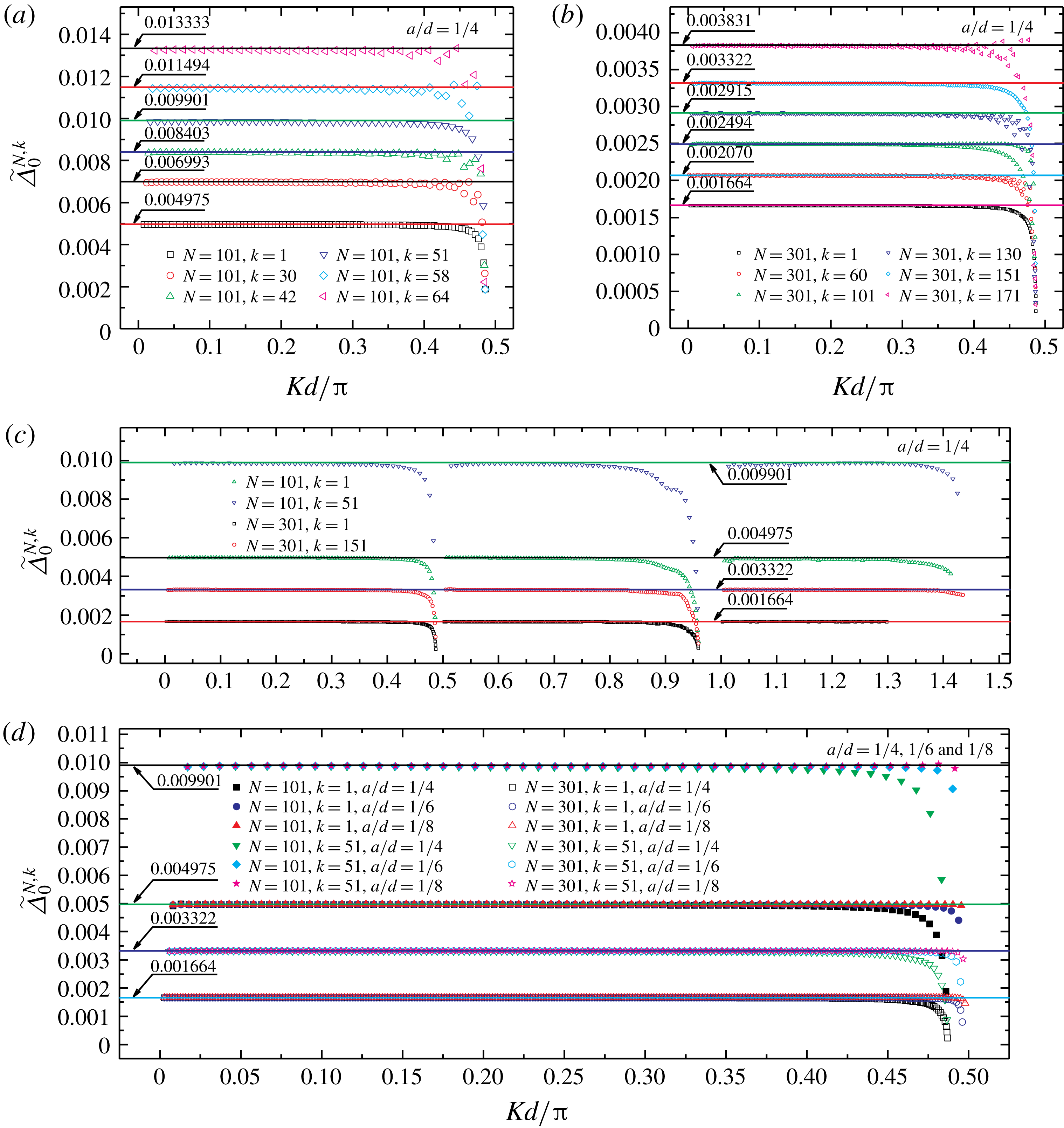
in figure 5. The discrete points in the figure were obtained as follows: for wave load curves (e.g. figures 1, 3 and 4), we first calculated the average value and difference of the abscissae of two adjacent local maxima (or minima) points (i.e. the mean and the difference of the values of
 $Kd/\unicode[STIX]{x03C0}$
corresponding to two adjacent local maxima (or minima) points). Second, we took the mean as the abscissae and the difference in the same pair of
 $Kd/\unicode[STIX]{x03C0}$
as the ordinate of a discrete point in figure 5. Subsequently, we obtained the scatter plot of
 $\widetilde{\unicode[STIX]{x1D6E5}}_{0}^{N,k}$
versus
 $Kd/\unicode[STIX]{x03C0}$
. The variations in fluctuation spacing of the
 $k$
th (
 $k=1$
, 30, 42, 51, 58 and 64) cylinder in a long array (
 $N=101$
) in head waves (
 $\unicode[STIX]{x1D6FD}=0$
) are shown in figure 5(a). Spacing
 $\widetilde{\unicode[STIX]{x1D6E5}}_{0}^{N,k}$
is almost constant in Region III for each cylinder. The constants are shown by solid lines of different colours in the figure. By contrast,
 $\widetilde{\unicode[STIX]{x1D6E5}}_{0}^{N,k}$
decreases with
 $Kd/\unicode[STIX]{x03C0}$
in Region II. The examples pertaining to
 $N=301$
and
 $k=1$
, 60, 101, 130, 151 and 171 are shown in figure 5(b). The examples of the first and the middle cylinder of two different arrays (
 $N=101$
, 301) are shown in figure 5(c). The same observation can be made from figure 5(b,c). To summarize, figure 5(a–c) shows that the fluctuation spacing does not change with
 $Kd/\unicode[STIX]{x03C0}$
in Region III; it decreases with an increase in the total number of cylinders
 $N$
; and it increases with the identification number
 $k$
. The plot of
 $\widetilde{\unicode[STIX]{x1D6E5}}_{0}^{N,k}$
versus
 $Kd/\unicode[STIX]{x03C0}$
for different diameter-to-spacing ratios
 $a/d$
is shown in figure 5(d), where
 $a/d=1/4$
,
 $1/6$
,
 $1/8$
;
 $N=101$
,
 $k=1$
, 51;
 $N=301$
,
 $k=1$
, 151. Figure 5(d) shows that, in Region III, the fluctuation spacing is independent of diameter-to-spacing ratio.
Measured value of fluctuation spacing
 $\widetilde{\unicode[STIX]{x1D6E5}}_{0}^{N,k}$
for the
 $k$
th cylinder of an array consisting of
 $N$
cylinders in head waves (
 $\unicode[STIX]{x1D6FD}=0$
).

The phenomenon discussed above is not a special case. Many cases of arrays with different parameter combinations of
 $N$
,
 $a/d$
and
 $\unicode[STIX]{x1D6FD}$
have been calculated (examples pertaining to
 $\unicode[STIX]{x1D6FD}\neq 0$
are given in the following sections). The computations strongly suggest that in Region III, the fluctuation spacing
 $\unicode[STIX]{x1D6E5}$
depends only on the total number of cylinders
 $N$
, cylinder position (identification number
 $k$
) and incidence angle
 $\unicode[STIX]{x1D6FD}$
;
 $\unicode[STIX]{x1D6E5}$
was found to be independent of the non-dimensional wavenumber
 $Kd/\unicode[STIX]{x03C0}$
and diameter-to-spacing ratio
 $a/d$
. This seems to be a general phenomenon. To the authors’ knowledge, this phenomenon has not been reported previously. In the following sections, we show that the mechanism associated with the phenomenon of constant fluctuation spacing in Region III is radically different from that associated with the spikes and secondary peaks/troughs in Regions I and II.
3 Derivation of formulae for fluctuation spacings in Region III based on interaction theory
The present study is conducted in the context of the linearized theory of time-harmonic water waves. Assuming a time factor
 $\text{e}^{-\text{i}\unicode[STIX]{x1D714}t}$
with angular frequency
 $\unicode[STIX]{x1D714}$
, the velocity potential can be expressed as
 $\unicode[STIX]{x1D6F7}(x,y,z,t)=\text{Re}\{\unicode[STIX]{x1D719}(x,y)f(z)\text{e}^{-\text{i}\unicode[STIX]{x1D714}t}\}$
. Plane
 $Oxy$
is the still water surface; the positive z-axis points vertically upwards; and
 $-h<z<0$
is the fluid domain, where h is the depth. Linton & Evans (Reference Linton and Evans1990) devised simple formulae for determining the wave field near a cylinder and the wave force on the cylinder in an array of bottom-mounted cylinders with arbitrary geometric arrangement. Their coordinate system is shown in figure 2(b). Following Linton & Evans (Reference Linton and Evans1990), we consider the diffraction by a straight-line array of
 $N$
identical bottom-mounted circular cylinders and list a few major formulae used in this study. The spatial factor of velocity potential near cylinder
 $k$
is expressed as follows:
 $$\begin{eqnarray}\unicode[STIX]{x1D719}(r_{k},\unicode[STIX]{x1D703}_{k})=\mathop{\sum }_{n=-\infty }^{\infty }A_{n}^{k}\text{e}^{\text{i}n\unicode[STIX]{x1D703}_{k}}[Z_{n}\text{H}_{n}(Kr_{k})-\text{J}_{n}(Kr_{k})],\end{eqnarray}$$
where
 $r_{k}$
,
 $\unicode[STIX]{x1D703}_{k}$
are shown in figure 2(b). Wavenumber
 $K$
satisfies the dispersion relationship
 $\unicode[STIX]{x1D714}^{2}=gK\tanh Kh$
, where
 $g$
denotes gravitational acceleration. Function
 $\text{H}_{n}$
is the
 $n$
th-order Hankel function of the first kind,
 $\text{J}_{n}$
the
 $n$
th-order Bessel functions of the first kind and
 $Z_{n}=\text{J}_{n}^{\prime }(Ka)/\text{H}_{n}^{\prime }(Ka)$
. Here
 $A_{n}^{k}$
is an unknown coefficient of cylinder
 $k$
. The linear system of equations for solving
 $A_{n}^{k}$
is
 $$\begin{eqnarray}A_{n}^{k}+\mathop{\sum }_{\substack{ j=1 \\ j\neq k}}^{N}\mathop{\sum }_{m=-\infty }^{\infty }A_{m}^{j}Z_{m}\text{H}_{m-n}(KR_{jk})\text{e}^{\text{i}(m-n)\unicode[STIX]{x1D6FC}_{jk}}=-I_{k}\text{e}^{\text{i}n((\unicode[STIX]{x03C0}/2)-\unicode[STIX]{x1D6FD})}.\end{eqnarray}$$
Here,
 $I_{k}=\text{e}^{\text{i}2d(k-1)K\cos \unicode[STIX]{x1D6FD}}$
is a phase factor associated with the
 $k$
th cylinder,
 $R_{jk}$
is the distance between the axes of cylinders
 $j$
and
 $k$
and
 $\unicode[STIX]{x1D6FC}_{jk}$
is the angle between the
 $x$
-axis and the line connecting the points of intersection of the axes of cylinders and the plane
 $Oxy$
, as shown in figure 2(b). The time-independent factor of the wave force acting on cylinder
 $k$
is
 $$\begin{eqnarray}\boldsymbol{F}^{k}=\left\{\begin{array}{@{}c@{}}F_{x}^{k}\\ F_{y}^{k}\end{array}\right\}=-\frac{2\unicode[STIX]{x1D70C}g\widetilde{A}\tanh Kh}{K^{2}\text{H}_{1}^{\prime }(Ka)}\left\{\begin{array}{@{}c@{}}\text{i}(A_{-1}^{k}-A_{1}^{k})\\ A_{-1}^{k}+A_{1}^{k}\end{array}\right\},\end{eqnarray}$$
where
 $\unicode[STIX]{x1D70C}$
is the fluid density and
 $\widetilde{A}$
the amplitude of the incident wave. The dimensionless wave force
 $\boldsymbol{X}^{k}$
normalized against that of a single isolated cylinder is
 $$\begin{eqnarray}\boldsymbol{X}^{k}=\left\{\begin{array}{@{}c@{}}X_{x}^{k}\\ X_{y}^{k}\end{array}\right\}=-\frac{1}{2}\left\{\begin{array}{@{}c@{}}\text{i}(A_{-1}^{k}-A_{1}^{k})\\ A_{-1}^{k}+A_{1}^{k}\end{array}\right\}.\end{eqnarray}$$
Here, the subscripts
 $x$
and
 $y$
refer to the force along the
 $x$
and
 $y$
directions, respectively. We can investigate fluctuations in the magnitude of the wave force by studying the coefficients
 $A_{1}^{k}$
and
 $A_{-1}^{k}$
. To understand the characteristics of the unknown coefficients holistically, calculations were performed for determining
 $A_{n}^{k}$
. Our computations show that variations in
 $|A_{n}^{k}|$
with
 $Kd/\unicode[STIX]{x03C0}$
are similar to those in the magnitude of wave loads;
 $|A_{n}^{k}|$
fluctuates with
 $Kd/\unicode[STIX]{x03C0}$
, and the fluctuation spacing in Region III is constant. All fluctuation characteristics of
 $|A_{n}^{k}|$
are identical, as shown in the following subsection.
3.1 Fluctuations of
 $|A_{n}^{k}|$
,
$|_{c}D_{n}^{k}|$
and
${\mathcal{D}}_{n}^{k}$


We rewrite (3.2) in matrix form, as follows:
 $$\begin{eqnarray}\unicode[STIX]{x1D63F}\boldsymbol{A}=\boldsymbol{B},\end{eqnarray}$$
where
 $$\begin{eqnarray}\displaystyle \boldsymbol{A} & = & \displaystyle \left[\ldots ,A_{-n}^{1},\ldots ,A_{-1}^{1},A_{0}^{1},A_{1}^{1},\ldots ,A_{n}^{1},\ldots ,A_{-n}^{2},\ldots ,A_{-1}^{2},A_{0}^{2},A_{1}^{2},\ldots ,A_{n}^{2},\ldots ,\right.\nonumber\\ \displaystyle & & \displaystyle \quad \left.A_{-n}^{k},\ldots ,A_{-1}^{k},A_{0}^{k},A_{1}^{k},\ldots ,A_{n}^{k},\ldots ,A_{-n}^{N},\ldots ,A_{-1}^{N},A_{0}^{N},A_{1}^{N},\ldots ,A_{n}^{N},\ldots \right]^{T}\nonumber\\ \displaystyle & & \displaystyle\end{eqnarray}$$
and
 $\unicode[STIX]{x1D63F}(\boldsymbol{B})$
is the coefficient matrix (column vector) of the left (right)-hand side of (3.2).
According to Cramer’s rule,
 $$\begin{eqnarray}A_{n}^{k}={\text{}_{c}D}_{n}^{k}/D,\end{eqnarray}$$
where
 $D$
is the determinant of
 $\unicode[STIX]{x1D63F}$
,
 ${\text{}_{c}D}_{n}^{k}$
is the determinant of the matrix
 $\unicode[STIX]{x1D63F}_{n}^{k}$
and
 $\unicode[STIX]{x1D63F}_{n}^{k}$
is obtained from
 $\unicode[STIX]{x1D63F}$
by replacing the corresponding column with
 $\boldsymbol{B}$
. We executed a large number of computation runs with different parameter combinations. The results show that the fluctuation spacings of
 $|A_{n}^{k}|$
and
 $|{\text{}_{c}D}_{n}^{k}|$
are independent of
 $n$
, and a few examples are shown in figure 6(a,b). Moreover, the results show that the fluctuation phenomenon of
 $|A_{n}^{k}|$
can be attributed completely to
 $|{\text{}_{c}D}_{n}^{k}|$
, as examples show in figure 6(b). In figure 6, the notation
 $\widetilde{\unicode[STIX]{x1D6E5}}_{\unicode[STIX]{x1D6FD}}^{N,k}$
for the fluctuation spacing of the magnitude of wave load is also used to denote the measured value of fluctuation spacing for
 $|A_{n}^{k}|$
and
 $|{\text{}_{c}D}_{n}^{k}|$
; the total number of cylinders in the array is
 $N=101$
, diameter-to-spacing ratio
 $a/d=1/4$
and incidence angle
 $\unicode[STIX]{x1D6FD}=0$
. Similar to figure 5, the abscissae and ordinates of the discrete points and solid lines in figure 6 are the mean and the difference of the values of
 $Kd/\unicode[STIX]{x03C0}$
corresponding to two adjacent local maximum (or minimum) points. Computations suggest that the fluctuation spacing of
 $|A_{n}^{k}|$
is equal to that of
 $|{\text{}_{c}D}_{n}^{k}|$
. As shown in figure 6(a,b), the fluctuation spacings of
 $|A_{\pm 1}^{k}|$
,
 $|A_{n}^{k}|$
and
 $|{\text{}_{c}D}_{n}^{k}|$
are identical. Then, we study the fluctuation of
 $|{\text{}_{c}D}_{n}^{k}|$
, although it is adequate to consider
 $|A_{\pm 1}^{k}|$
for the sake of understanding the fluctuation characteristics of wave loads.
According to the definition of determinant based on Laplace expansion (or equivalently expressed in terms of the Levi-Civita symbol),
 ${\text{}_{c}D}_{n}^{k}$
can be expressed as the sum of many terms:
 $$\begin{eqnarray}{\text{}_{c}D}_{n}^{k}={\text{}_{0}D}_{n}^{k}+{\text{}_{1}D}_{n}^{k}+{\text{}_{h}D}_{n}^{k}.\end{eqnarray}$$
Here
 ${\text{}_{0}D}_{n}^{k}$
is the term without Hankel function,
 ${\text{}_{1}D}_{n}^{k}$
is the sum of all terms containing only one Hankel function and
 ${\text{}_{h}D}_{n}^{k}$
is the sum of all terms containing the products of multiple Hankel functions. Our computations show that
 ${\text{}_{h}D}_{n}^{k}$
has little effect on the fluctuation spacing of
 $|{\text{}_{c}D}_{n}^{k}|$
in Region III. A few examples are shown in figure 6(c). It can be observed that in Region III, the fluctuation spacing of
 $|{\text{}_{c}D}_{n}^{k}|$
is consistent with that of
 $|{\text{}_{l}D}_{n}^{k}|$
, where
 ${\text{}_{l}D}_{n}^{k}={\text{}_{0}D}_{n}^{k}+{\text{}_{1}D}_{n}^{k}$
. The inconsistencies in fluctuation spacing between
 $|{\text{}_{c}D}_{n}^{k}|$
and
 $|{\text{}_{l}D}_{n}^{k}|$
occur only in Regions I and II, which are not objects of interest in this study. Therefore, it is adequate to study
 $|{\text{}_{l}D}_{n}^{k}|$
if the fluctuation spacing of
 $|{\text{}_{c}D}_{n}^{k}|$
in Region III alone is of concern. The expression of
 ${\text{}_{l}D}_{n}^{k}$
is
 $$\begin{eqnarray}{\text{}_{l}D}_{n}^{k}(\unicode[STIX]{x1D705})=-I_{k}\text{e}^{\text{i}n((\unicode[STIX]{x03C0}/2)-\unicode[STIX]{x1D6FD})}+\mathop{\sum }_{\substack{ j=1 \\ j\neq k}}^{N}\mathop{\sum }_{m=-\infty }^{\infty }I_{j}\text{e}^{\text{i}m((\unicode[STIX]{x03C0}/2)-\unicode[STIX]{x1D6FD})}Z_{m}\text{H}_{m-n}(KR_{jk})\text{e}^{\text{i}(m-n)\unicode[STIX]{x1D6FC}_{jk}},\end{eqnarray}$$
where
 $\unicode[STIX]{x1D705}=Kd/\unicode[STIX]{x03C0}$
. To obtain the analytical solution, substituting the asymptotic expression of Hankel function into (3.9), then
 ${\text{}_{l}D}_{n}^{k}(\unicode[STIX]{x1D705})$
can be changed into
 ${\text{}_{la}D}_{n}^{k}(\unicode[STIX]{x1D705})$
as follows:
 $$\begin{eqnarray}\displaystyle {\text{}_{la}D}_{n}^{k}(\unicode[STIX]{x1D705}) & = & \displaystyle -\text{exp}\left[\text{i}\left(2(k-1)\unicode[STIX]{x03C0}\unicode[STIX]{x1D705}\cos \unicode[STIX]{x1D6FD}+n\left(\frac{\unicode[STIX]{x03C0}}{2}-\unicode[STIX]{x1D6FD}\right)\right)\right]+\mathop{\sum }_{\substack{ j=1 \\ j\neq k}}^{N}\mathop{\sum }_{m=-\infty }^{\infty }\left\{\!\sqrt{1/(\unicode[STIX]{x1D705}\unicode[STIX]{x03C0}^{2}|j-k|)}\right.\nonumber\\ \displaystyle & & \displaystyle \text{}\times Z_{m}\text{exp}\left[\text{i}\left(2(j-1)\unicode[STIX]{x03C0}\unicode[STIX]{x1D705}\cos \unicode[STIX]{x1D6FD}+2|j-k|\unicode[STIX]{x03C0}\unicode[STIX]{x1D705}+m\left(\frac{\unicode[STIX]{x03C0}}{2}-\unicode[STIX]{x1D6FD}\right)+(m-n)\unicode[STIX]{x1D6FC}_{jk}\right.\right.\nonumber\\ \displaystyle & & \displaystyle \left.\left.\left.-\,\frac{(m-n)\unicode[STIX]{x03C0}}{2}-\frac{\unicode[STIX]{x03C0}}{4}\right)\right]\right\}.\end{eqnarray}$$
Fluctuation spacings of
 $|A_{n}^{k}|$
,
 $|{\text{}_{c}D}_{n}^{k}|$
,
 $|{\text{}_{l}D}_{n}^{k}|$
,
 $|{\text{}_{la}D}_{n}^{k}|$
and
 ${\mathcal{D}}_{n}^{k}$
for different Fourier modes
 $n$
against non-dimensional wavenumber
 $Kd/\unicode[STIX]{x03C0}$
. Here
 $N=101,k=1,\unicode[STIX]{x1D6FD}=0$
and
 $a/d=1/4$
.

For large
 $KR_{jk}$
, it is obvious that the asymptotic expression of Hankel function can give very accurate results. If this is not the case, the use of the asymptotic expression will affect the numerical accuracy of (3.9). However, this does not affect the fluctuation spacing of concern in this paper. Our computations show that the fluctuation spacing of
 $|{\text{}_{l}D}_{n}^{k}(\unicode[STIX]{x1D705})|$
is consistent with that of
 $|{\text{}_{la}D}_{n}^{k}(\unicode[STIX]{x1D705})|$
, as illustrated by several examples shown in figure 6(d). Figure 6(d) uses two ordinate axes with different starting points on the left- and right-hand sides of the graph. The comparison of fluctuation spacing between
 $|{\text{}_{l}D}_{n}^{k}(\unicode[STIX]{x1D705})|$
and
 $|{\text{}_{la}D}_{n}^{k}(\unicode[STIX]{x1D705})|$
is shown in the upper half of figure 6(d) (the part marked with (
 $d_{1}$
)) and the ordinate values of the corresponding points are obtained from the left-hand vertical axis. Therefore, it is adequate to study
 $|{\text{}_{la}D}_{n}^{k}(\unicode[STIX]{x1D705})|$
. It will be shown in the following sections that the formulae for fluctuation spacing derived using the asymptotic expression of
 $\text{H}_{m-n}(KR_{jk})$
can be applied to almost all
 $Kd/\unicode[STIX]{x03C0}$
in Region III.
It is evident that the abscissa of the local extreme points of
 $|{\text{}_{la}D}_{n}^{k}(\unicode[STIX]{x1D705})|$
corresponds to that of
 $|{\text{}_{la}D}_{n}^{k}(\unicode[STIX]{x1D705})|^{2}$
if
 $|{\text{}_{la}D}_{n}^{k}(\unicode[STIX]{x1D705})|$
is not zero. Our computations show that
 $|{\text{}_{la}D}_{n}^{k}(\unicode[STIX]{x1D705})|$
is always greater than zero, and there is no indication that
 $|{\text{}_{la}D}_{n}^{k}(\unicode[STIX]{x1D705})|$
is equal to zero in Region III. Then, to facilitate the derivation process, we consider
 $|{\text{}_{la}D}_{n}^{k}(\unicode[STIX]{x1D705})|^{2}$
instead of
 $|{\text{}_{la}D}_{n}^{k}(\unicode[STIX]{x1D705})|$
.
Here
 $|{\text{}_{la}D}_{n}^{k}(\unicode[STIX]{x1D705})|^{2}$
can be expressed as
 $|{\text{}_{la}D}_{n}^{k}(\unicode[STIX]{x1D705})|^{2}={\mathcal{D}}_{n}^{k}+_{h}{\mathcal{D}}_{n}^{k}$
. In Region III, omitting higher-order quantity
 $_{h}{\mathcal{D}}_{n}^{k}$
from
 $|{\text{}_{la}D}_{n}^{k}(\unicode[STIX]{x1D705})|^{2}$
, we can get
 ${\mathcal{D}}_{n}^{k}$
as follows:
 $$\begin{eqnarray}\displaystyle {\mathcal{D}}_{n}^{k}(\unicode[STIX]{x1D705}) & = & \displaystyle \unicode[STIX]{x1D709}(\unicode[STIX]{x1D705})-\mathop{\sum }_{\substack{ j=1 \\ j\neq k}}^{N}\mathop{\sum }_{m=-\infty }^{\infty }2\sqrt{1/(\unicode[STIX]{x1D705}\unicode[STIX]{x03C0}^{2}|j-k|)}\text{Re}(Z_{m})\cos \unicode[STIX]{x1D708}\nonumber\\ \displaystyle & & \displaystyle +\,\mathop{\sum }_{\substack{ j=1 \\ j\neq k}}^{N}\mathop{\sum }_{m=-\infty }^{\infty }2\sqrt{1/(\unicode[STIX]{x1D705}\unicode[STIX]{x03C0}^{2}|j-k|)}\text{Im}(Z_{m})\sin \unicode[STIX]{x1D708},\end{eqnarray}$$
where
 $$\begin{eqnarray}\displaystyle & \displaystyle \unicode[STIX]{x1D709}(\unicode[STIX]{x1D705})=1+\mathop{\sum }_{\substack{ j=1 \\ j\neq k}}^{N}\mathop{\sum }_{m=-\infty }^{\infty }[1/(\unicode[STIX]{x1D705}\unicode[STIX]{x03C0}^{2}|\,j-k|)]\{[\text{Re}(Z_{m})]^{2}+[\text{Im}(Z_{m})]^{2}\}, & \displaystyle\end{eqnarray}$$
 $$\begin{eqnarray}\displaystyle & \displaystyle \unicode[STIX]{x1D708}=2(j-k)\unicode[STIX]{x03C0}\unicode[STIX]{x1D705}\cos \unicode[STIX]{x1D6FD}+2|j-k|\unicode[STIX]{x03C0}\unicode[STIX]{x1D705}-(m-n)\unicode[STIX]{x1D6FD}+(m-n)\unicode[STIX]{x1D6FC}_{jk}-\frac{\unicode[STIX]{x03C0}}{4}. & \displaystyle\end{eqnarray}$$
Here
 $_{h}{\mathcal{D}}_{n}^{k}$
is the sum of the following three types of expressions:
 $$\begin{eqnarray}\unicode[STIX]{x1D6F6}_{i}\sqrt{1/\left[(\unicode[STIX]{x1D705}\unicode[STIX]{x03C0}^{2})^{2}|j_{1}-k||j_{2}-k|\right]}\sin (\unicode[STIX]{x1D708}_{2}-\unicode[STIX]{x1D708}_{1}+\unicode[STIX]{x1D6E9}_{i})\quad (i=1,2,3),\end{eqnarray}$$
where
 $\unicode[STIX]{x1D6F6}_{1}=\text{Re}(Z_{m_{1}})\text{Im}(Z_{m_{2}})$
,
 $\unicode[STIX]{x1D6F6}_{2}=\text{Re}(Z_{m_{1}})\text{Re}(Z_{m_{2}})$
,
 $\unicode[STIX]{x1D6F6}_{3}=\text{Im}(Z_{m_{1}})\text{Im}(Z_{m_{2}})$
;
 $\unicode[STIX]{x1D6E9}_{1}=0$
,
 $\unicode[STIX]{x1D6E9}_{2}=\unicode[STIX]{x1D6E9}_{3}=\unicode[STIX]{x03C0}/2$
;
 $m_{1}$
and
 $m_{2}$
(
 $j_{1}$
and
 $j_{2}$
) are summation indices, and their lower and upper bounds of summation are the same,
 $-\infty$
and
 $\infty$
(1 and
 $N$
), respectively. Also,
 $\unicode[STIX]{x1D708}_{1}$
(
 $\unicode[STIX]{x1D708}_{2}$
) is determined by substituting
 $m_{1}$
and
 $j_{1}$
(
 $m_{2}$
and
 $j_{2}$
) into (3.13).
Nearly all the terms represented by these three types of expressions are obviously smaller than those in the series of (3.11). In Region III, the sum of the three types of terms is a higher-order small quantity and does not affect the fluctuation spacing, which is confirmed by our computations. As illustrated by several examples shown in figure 6(d), the fluctuation spacing of
 $|{\text{}_{la}D}_{n}^{k}(\unicode[STIX]{x1D705})|$
is consistent with that of
 ${\mathcal{D}}_{n}^{k}(\unicode[STIX]{x1D705})$
. The comparison of fluctuation spacing between
 $|{\text{}_{la}D}_{n}^{k}(\unicode[STIX]{x1D705})|$
and
 ${\mathcal{D}}_{n}^{k}(\unicode[STIX]{x1D705})$
is shown in the lower half of figure 6(d) (the part marked with (
 $d_{2}$
)) and the ordinate values of the corresponding points are obtained from the right-hand vertical axis. Therefore, it is adequate to study
 ${\mathcal{D}}_{n}^{k}(\unicode[STIX]{x1D705})$
for the fluctuation spacing of concern in this paper.
It is apparent that the term related to the fluctuation with
 $\unicode[STIX]{x1D705}$
is
 $2(j-k)\unicode[STIX]{x03C0}\unicode[STIX]{x1D705}\cos \unicode[STIX]{x1D6FD}+2|j-k|\unicode[STIX]{x03C0}\unicode[STIX]{x1D705}$
, which does not contain
 $n$
. The term containing
 $n$
is
 $-(m-n)\unicode[STIX]{x1D6FD}+(m-n)\unicode[STIX]{x1D6FC}_{jk}$
, which is independent of
 $\unicode[STIX]{x1D705}$
. This term does not contribute to the fluctuation with
 $\unicode[STIX]{x1D705}$
. Therefore, the fluctuation spacings of
 ${\mathcal{D}}_{n}^{k}(\unicode[STIX]{x1D705})$
for different
 $n$
are identical, provided the same cylinder
 $k$
is considered. This agrees with the results mentioned earlier in this subsection.
3.2 Formula for predicting fluctuation spacing in head waves
3.2.1 Formulation
In this subsection, we consider the situation of a cylinder array in head waves (
 $\unicode[STIX]{x1D6FD}=0$
). It is an important operating condition and can provide insights into rules for variations in the fluctuation of wave loads. A simple formula is presented for determining the fluctuation spacing of the magnitude of wave loads.
Evidently, the wave force in the
 $y$
-direction is
 $X_{y}^{k}=0$
in head waves (
 $\unicode[STIX]{x1D6FD}=0$
), which gives
 $A_{-1}^{k}=-A_{1}^{k}$
. Then, the wave load on the
 $k$
th cylinder in the
 $x$
-direction is
 $X_{x}^{k}=\text{i}A_{1}^{k}$
. The fluctuation of
 $|X_{x}^{k}|$
is equivalent to that of
 $|A_{1}^{k}|$
. As shown in § 3.1, the fluctuation spacings of
 $|A_{\pm 1}^{k}|$
,
 $|A_{n}^{k}|$
,
 $|_{c}D_{n}^{k}|$
and
 ${\mathcal{D}}_{n}^{k}$
are identical. Therefore, we analysed the fluctuation spacing of the magnitude of wave load by studying the horizontal distance between the two adjacent maximum/minimum points of
 ${\mathcal{D}}_{n}^{k}(\unicode[STIX]{x1D705})$
.
The substitution of
 $\unicode[STIX]{x1D6FD}=0$
into (3.11) yielded
 $$\begin{eqnarray}{\mathcal{D}}_{n}^{k}(\unicode[STIX]{x1D705})=\widetilde{\unicode[STIX]{x1D709}}(\unicode[STIX]{x1D705})\pm \sqrt{(\unicode[STIX]{x1D709}_{1}^{\unicode[STIX]{x03C0}})^{2}+(\unicode[STIX]{x1D709}_{2}^{\unicode[STIX]{x03C0}})^{2}}\mathop{\sum }_{j=k+1}^{N}\sqrt{\frac{1}{j-k}}\cos \left[4(j-k)\unicode[STIX]{x03C0}\unicode[STIX]{x1D705}+\unicode[STIX]{x1D6FC}(\unicode[STIX]{x1D705})\right],\end{eqnarray}$$
‘
 $+$
’ for
 $\unicode[STIX]{x1D709}_{1}^{\unicode[STIX]{x03C0}}<0$
, ‘
 $-$
’ for
 $\unicode[STIX]{x1D709}_{1}^{\unicode[STIX]{x03C0}}>0$
, where
 $$\begin{eqnarray}\unicode[STIX]{x1D6FC}(\unicode[STIX]{x1D705})=\arctan \frac{\unicode[STIX]{x1D709}_{2}^{\unicode[STIX]{x03C0}}}{\unicode[STIX]{x1D709}_{1}^{\unicode[STIX]{x03C0}}},\quad -\frac{\unicode[STIX]{x03C0}}{2}<\unicode[STIX]{x1D6FC}(\unicode[STIX]{x1D705})<\frac{\unicode[STIX]{x03C0}}{2},\end{eqnarray}$$
 $$\begin{eqnarray}\widetilde{\unicode[STIX]{x1D709}}(\unicode[STIX]{x1D705})=\unicode[STIX]{x1D709}(\unicode[STIX]{x1D705})-\unicode[STIX]{x1D709}_{1}^{0}(\unicode[STIX]{x1D705})\mathop{\sum }_{j=1}^{k-1}\sqrt{\frac{1}{k-j}},\end{eqnarray}$$
 $$\begin{eqnarray}\displaystyle \unicode[STIX]{x1D709}_{1}^{\unicode[STIX]{x1D6FC}_{jk}}(\unicode[STIX]{x1D705}) & = & \displaystyle \frac{2}{\unicode[STIX]{x03C0}}\sqrt{\frac{1}{\unicode[STIX]{x1D705}}}\mathop{\sum }_{m=-\infty }^{\infty }\left\{\text{Re}(Z_{m})\cos \left[(m-n)\unicode[STIX]{x1D6FC}_{jk}-\frac{\unicode[STIX]{x03C0}}{4}\right]\right.\nonumber\\ \displaystyle & & \displaystyle \left.-\,\text{Im}(Z_{m})\sin \left[(m-n)\unicode[STIX]{x1D6FC}_{jk}-\frac{\unicode[STIX]{x03C0}}{4}\right]\right\},\end{eqnarray}$$
 $$\begin{eqnarray}\displaystyle \unicode[STIX]{x1D709}_{2}^{\unicode[STIX]{x1D6FC}_{jk}}(\unicode[STIX]{x1D705}) & = & \displaystyle \frac{2}{\unicode[STIX]{x03C0}}\sqrt{\frac{1}{\unicode[STIX]{x1D705}}}\mathop{\sum }_{m=-\infty }^{\infty }\left\{\text{Re}(Z_{m})\sin \left[(m-n)\unicode[STIX]{x1D6FC}_{jk}-\frac{\unicode[STIX]{x03C0}}{4}\right]\right.\nonumber\\ \displaystyle & & \displaystyle \left.+\,\text{Im}(Z_{m})\cos \left[(m-n)\unicode[STIX]{x1D6FC}_{jk}-\frac{\unicode[STIX]{x03C0}}{4}\right]\right\}.\end{eqnarray}$$
In the series of expression (3.15),
 $k=1,2,\ldots ,N-1$
. For
 $k=N$
,
 ${\mathcal{D}}_{n}^{k}(\unicode[STIX]{x1D705})=\widetilde{\unicode[STIX]{x1D709}}(\unicode[STIX]{x1D705})$
. The lower and upper bounds of summation in (3.15) are
 $k+1$
and
 $N$
, respectively. This means that only the cylinders downstream of cylinder
 $k$
contribute to
 ${\mathcal{D}}_{n}^{k}(\unicode[STIX]{x1D705})$
for
 $\unicode[STIX]{x1D6FD}=0$
.
(a) Numerical values of
 $\widetilde{\unicode[STIX]{x1D709}}(\unicode[STIX]{x1D705})$
,
 $\sqrt{(\unicode[STIX]{x1D709}_{1}^{\unicode[STIX]{x03C0}})^{2}+(\unicode[STIX]{x1D709}_{2}^{\unicode[STIX]{x03C0}})^{2}}$
,
 $\unicode[STIX]{x1D70F}_{1}(\unicode[STIX]{x1D705})$
,
 $\unicode[STIX]{x1D70F}_{2}(\unicode[STIX]{x1D705})$
,
 ${\mathcal{D}}_{n}^{k}(\unicode[STIX]{x1D705})-\widetilde{\unicode[STIX]{x1D709}}(\unicode[STIX]{x1D705})$
and
 ${\mathcal{D}}_{n}^{k}(\unicode[STIX]{x1D705})$
. (b) Values of
 $Kd/\unicode[STIX]{x03C0}$
corresponding to each local maximum point for
 ${\mathcal{D}}_{n}^{k}(\unicode[STIX]{x1D705})$
,
 ${\mathcal{D}}_{n}^{k}(\unicode[STIX]{x1D705})-\widetilde{\unicode[STIX]{x1D709}}(\unicode[STIX]{x1D705})$
,
 $\unicode[STIX]{x1D70F}_{2}(\unicode[STIX]{x1D705})$
and
 $\unicode[STIX]{x1D70F}_{1}(\unicode[STIX]{x1D705})$
. Here
 $N=21,k=11$
and
 $n=1$
.

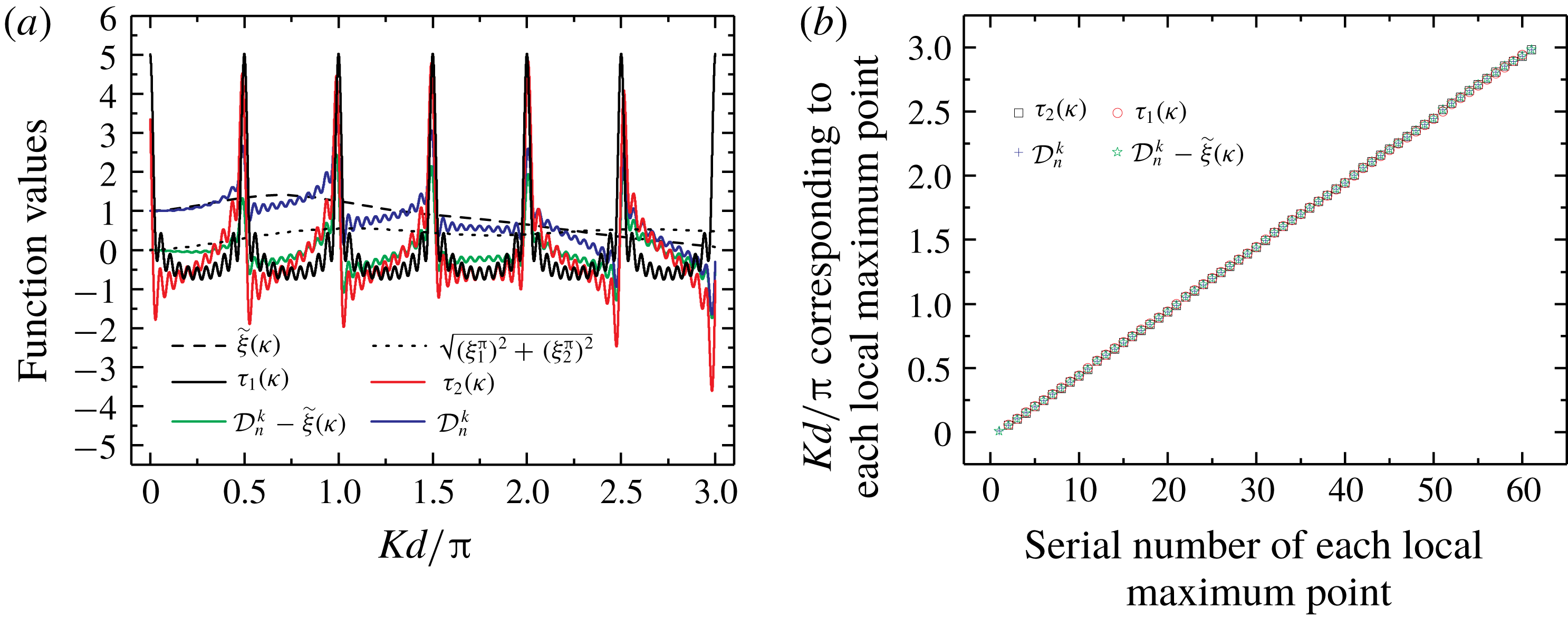
A large number of calculations for cases with different parameter combinations were performed. An example is shown in figure 7, where
 $N=21,k=11$
and
 $n=1$
. The results show that
 $\widetilde{\unicode[STIX]{x1D709}}(\unicode[STIX]{x1D705})$
only changes the numerical value of
 ${\mathcal{D}}_{n}^{k}(\unicode[STIX]{x1D705})$
, but it does not change the positions of the extremum points of
 ${\mathcal{D}}_{n}^{k}(\unicode[STIX]{x1D705})$
. The horizontal distance between the two adjacent local maxima/minima points of
 ${\mathcal{D}}_{n}^{k}(\unicode[STIX]{x1D705})$
depends entirely on the second term of (3.15). Figure 7(a) shows the numerical values of
 $\widetilde{\unicode[STIX]{x1D709}}(\unicode[STIX]{x1D705})$
,
 ${\mathcal{D}}_{n}^{k}(\unicode[STIX]{x1D705})$
and
 ${\mathcal{D}}_{n}^{k}(\unicode[STIX]{x1D705})-\widetilde{\unicode[STIX]{x1D709}}(\unicode[STIX]{x1D705})$
. It is apparent that
 $\widetilde{\unicode[STIX]{x1D709}}(\unicode[STIX]{x1D705})$
is a slowly varying function. Functions
 ${\mathcal{D}}_{n}^{k}(\unicode[STIX]{x1D705})$
and
 ${\mathcal{D}}_{n}^{k}(\unicode[STIX]{x1D705})-\widetilde{\unicode[STIX]{x1D709}}(\unicode[STIX]{x1D705})$
are rapidly oscillating functions that are responsible for the fluctuation phenomenon studied in the present work. Figure 7(b) shows the abscissa of each local maximum point of
 ${\mathcal{D}}_{n}^{k}(\unicode[STIX]{x1D705})$
and
 ${\mathcal{D}}_{n}^{k}(\unicode[STIX]{x1D705})-\widetilde{\unicode[STIX]{x1D709}}(\unicode[STIX]{x1D705})$
. The ordinate of figure 7(b) is the value of
 $Kd/\unicode[STIX]{x03C0}$
corresponding to each local maximum point, and the abscissa of figure 7(b) is the serial number of each local maximum point. The linear relationship shown in figure 7(b) will be explained in § 4. Figure 7(b) shows that the abscissae of the local maximum points of
 ${\mathcal{D}}_{n}^{k}(\unicode[STIX]{x1D705})-\widetilde{\unicode[STIX]{x1D709}}(\unicode[STIX]{x1D705})$
coincide with those of
 ${\mathcal{D}}_{n}^{k}(\unicode[STIX]{x1D705})$
. In addition, it is observed that the abscissae of the local minimum points of
 ${\mathcal{D}}_{n}^{k}(\unicode[STIX]{x1D705})-\widetilde{\unicode[STIX]{x1D709}}(\unicode[STIX]{x1D705})$
coincide with those of
 ${\mathcal{D}}_{n}^{k}(\unicode[STIX]{x1D705})$
. For brevity, the plot for local minimum points similar to figure 7(b) is not shown. This suggests that
 $\widetilde{\unicode[STIX]{x1D709}}(\unicode[STIX]{x1D705})$
has no effect on the fluctuation spacing of
 ${\mathcal{D}}_{n}^{k}(\unicode[STIX]{x1D705})$
. Similarly, as shown in figure 7(a),
 $\sqrt{(\unicode[STIX]{x1D709}_{1}^{\unicode[STIX]{x03C0}})^{2}+(\unicode[STIX]{x1D709}_{2}^{\unicode[STIX]{x03C0}})^{2}}$
is a slowly varying function and does not affect the fluctuation spacing. Ignoring
 $\sqrt{(\unicode[STIX]{x1D709}_{1}^{\unicode[STIX]{x03C0}})^{2}+(\unicode[STIX]{x1D709}_{2}^{\unicode[STIX]{x03C0}})^{2}}$
, we consider the expression
 $$\begin{eqnarray}\unicode[STIX]{x1D70F}_{2}(\unicode[STIX]{x1D705})=\pm \mathop{\sum }_{j=k+1}^{N}\sqrt{\frac{1}{j-k}}\cos \left[4(j-k)\unicode[STIX]{x03C0}\unicode[STIX]{x1D705}+\unicode[STIX]{x1D6FC}(\unicode[STIX]{x1D705})\right].\end{eqnarray}$$
The numerical values of
 $\unicode[STIX]{x1D70F}_{2}(\unicode[STIX]{x1D705})$
are shown in figure 7(a). The value of
 $Kd/\unicode[STIX]{x03C0}$
corresponding to each local maximum point of
 $\unicode[STIX]{x1D70F}_{2}(\unicode[STIX]{x1D705})$
is shown in figure 7(b). The plot for the local minimum points is not shown for brevity. It is observed that the abscissae of the extremum points of
 $\unicode[STIX]{x1D70F}_{2}(\unicode[STIX]{x1D705})$
coincide with those of
 ${\mathcal{D}}_{n}^{k}(\unicode[STIX]{x1D705})$
. It remains difficult to find the analytical solution of the horizontal spacing between the two adjacent local maximum/minimum points for
 $\unicode[STIX]{x1D70F}_{2}(\unicode[STIX]{x1D705})$
. Our computations show that
 $|\unicode[STIX]{x1D6FC}(\unicode[STIX]{x1D705})|\ll 4(j-k)\unicode[STIX]{x03C0}\unicode[STIX]{x1D705}$
, where
 $\unicode[STIX]{x1D6FC}(\unicode[STIX]{x1D705})$
can be regarded a constant relative to
 $4(j-k)\unicode[STIX]{x03C0}\unicode[STIX]{x1D705}$
, which increases rapidly with
 $\unicode[STIX]{x1D705}$
. If
 $\unicode[STIX]{x1D6FC}(\unicode[STIX]{x1D705})$
is ignored,
 $\cos [4(j-k)\unicode[STIX]{x03C0}\unicode[STIX]{x1D705}+\unicode[STIX]{x1D6FC}(\unicode[STIX]{x1D705})]$
becomes
 $\cos [4(j-k)\unicode[STIX]{x03C0}\unicode[STIX]{x1D705}]$
. The two functions
 $\cos [4(j-k)\unicode[STIX]{x03C0}\unicode[STIX]{x1D705}]$
and
 $\cos [4(j-k)\unicode[STIX]{x03C0}\unicode[STIX]{x1D705}+\unicode[STIX]{x1D6FC}(\unicode[STIX]{x1D705})]$
have the same shape, except for a small translation. The horizontal spacing between the two adjacent local maximum/minimum points of
 $\cos [4(j-k)\unicode[STIX]{x03C0}\unicode[STIX]{x1D705}]$
coincides with that of
 $\cos [4(j-k)\unicode[STIX]{x03C0}\unicode[STIX]{x1D705}+\unicode[STIX]{x1D6FC}(\unicode[STIX]{x1D705})]$
. Then, we consider the expression
 $$\begin{eqnarray}\unicode[STIX]{x1D70F}_{1}(\unicode[STIX]{x1D705})=\mathop{\sum }_{j=k+1}^{N}\sqrt{\frac{1}{j-k}}\cos [4(j-k)\unicode[STIX]{x03C0}\unicode[STIX]{x1D705}].\end{eqnarray}$$
The value of
 $Kd/\unicode[STIX]{x03C0}$
corresponding to each local maximum point of
 $\unicode[STIX]{x1D70F}_{1}(\unicode[STIX]{x1D705})$
is shown in figure 7(b). The plot for the local minimum points is not shown for brevity. It is observed that the abscissae of the extremum points of
 $\unicode[STIX]{x1D70F}_{1}(\unicode[STIX]{x1D705})$
almost coincide with those of
 $\unicode[STIX]{x1D70F}_{2}(\unicode[STIX]{x1D705})$
and
 ${\mathcal{D}}_{n}^{k}(\unicode[STIX]{x1D705})$
. Therefore, the fluctuation spacing of
 ${\mathcal{D}}_{n}^{k}(\unicode[STIX]{x1D705})$
can be studied by considering
 $\unicode[STIX]{x1D70F}_{1}(\unicode[STIX]{x1D705})$
.
The problem studied herein is the fluctuation in Region III, where
 $Kd/\unicode[STIX]{x03C0}\neq \unicode[STIX]{x1D707}/2$
(
 $\unicode[STIX]{x1D707}$
is an integer) and
 $\sin 2\unicode[STIX]{x03C0}\unicode[STIX]{x1D705}\neq 0$
. Therefore, based on the product-to-sum identities of trigonometric functions, equation (3.21) can be re-expressed as
 $$\begin{eqnarray}\displaystyle \unicode[STIX]{x1D70F}_{1}(\unicode[STIX]{x1D705}) & = & \displaystyle \frac{1}{2\sin 2\unicode[STIX]{x03C0}\unicode[STIX]{x1D705}}\mathop{\sum }_{j=k+1}^{N}\sqrt{\frac{1}{j-k}}\{\sin [(4(j-k)+2)\unicode[STIX]{x03C0}\unicode[STIX]{x1D705}]-\sin [(4(j-k)-2)\unicode[STIX]{x03C0}\unicode[STIX]{x1D705}]\}\nonumber\\ \displaystyle & = & \displaystyle -\frac{1}{2}+\frac{1}{2\sin 2\unicode[STIX]{x03C0}\unicode[STIX]{x1D705}}\left\{\sqrt{\frac{1}{N-k}}\sin [(4(N-k)+2)\unicode[STIX]{x03C0}\unicode[STIX]{x1D705}]\right.\nonumber\\ \displaystyle & & \displaystyle \left.\text{}+\mathop{\sum }_{j=2}^{N-k}\left(\sqrt{\frac{1}{j-1}}-\sqrt{\frac{1}{j}}\right)\sin [(4(j-1)+2)\unicode[STIX]{x03C0}\unicode[STIX]{x1D705}]\right\}.\end{eqnarray}$$
Let
 $$\begin{eqnarray}\left(\sqrt{\frac{1}{j-1}}-\sqrt{\frac{1}{j}}\right)\sin [(4(j-1)+2)\unicode[STIX]{x03C0}\unicode[STIX]{x1D705}]=\unicode[STIX]{x1D700}(j,\unicode[STIX]{x1D705}).\end{eqnarray}$$
The quantity of interest is the horizontal distance between the two adjacent local maximum/minimum points (i.e. minimum fluctuation spacing). The minimum fluctuation spacing of
 $\unicode[STIX]{x1D70F}_{1}(\unicode[STIX]{x1D705})$
is mainly determined by
 $\sqrt{1/(N-k)}\sin [(4(N-k)+2)\unicode[STIX]{x03C0}\unicode[STIX]{x1D705}]$
. The reasons are as follows. When
 $N-k$
and
 $j$
are large, it is apparent that
 $\unicode[STIX]{x1D700}(j,\unicode[STIX]{x1D705})\rightarrow 0$
and
 $\unicode[STIX]{x1D700}(j,\unicode[STIX]{x1D705})$
does not contribute to
 $\unicode[STIX]{x1D70F}_{1}(\unicode[STIX]{x1D705})$
. When
 $N-k$
is large and
 $j$
is not large (i.e.
 $j-1$
is much smaller than
 $N-k$
),
 $\sin [(4(j-1)+2)\unicode[STIX]{x03C0}\unicode[STIX]{x1D705}]$
is a slowly varying function relative to the rapidly oscillating function
 $\sin [(4(N-k)+2)\unicode[STIX]{x03C0}\unicode[STIX]{x1D705}]$
. Then
 $\unicode[STIX]{x1D700}(j,\unicode[STIX]{x1D705})$
hardly affects the minimum fluctuation spacing of
 $\unicode[STIX]{x1D70F}_{1}(\unicode[STIX]{x1D705})$
, although it contributes to the value of
 $\unicode[STIX]{x1D70F}_{1}(\unicode[STIX]{x1D705})$
. Therefore,
 $\unicode[STIX]{x1D700}(j,\unicode[STIX]{x1D705})$
can be ignored if the only concern is the minimum fluctuation spacing. For
 $N-k=2,3$
, ignoring
 $\unicode[STIX]{x1D700}(j,\unicode[STIX]{x1D705})$
will lead to errors. The errors in fluctuation spacing for
 $N-k=2,3$
are 9.4 % and 5.7 %, respectively, if
 $\unicode[STIX]{x1D700}(j,\unicode[STIX]{x1D705})$
is ignored. When
 $N-k\geqslant 4$
, the errors are smaller than 1 %. Therefore, it is acceptable to ignore
 $\unicode[STIX]{x1D700}(j,\unicode[STIX]{x1D705})$
in most cases (
 $N-k\geqslant 4$
). In other words, it is adequate to consider
 $\unicode[STIX]{x1D70F}(\unicode[STIX]{x1D705})=\unicode[STIX]{x1D70F}_{1}(\unicode[STIX]{x1D705})-\sum _{j=2}^{N-k}\unicode[STIX]{x1D700}(j,\unicode[STIX]{x1D705}):$
 $$\begin{eqnarray}\unicode[STIX]{x1D70F}(\unicode[STIX]{x1D705})=-\frac{1}{2}+\frac{1}{2\sin 2\unicode[STIX]{x03C0}\unicode[STIX]{x1D705}}\sqrt{\frac{1}{N-k}}\sin \{[4(N-k)+2]\unicode[STIX]{x03C0}\unicode[STIX]{x1D705}\},\end{eqnarray}$$
if we focus on the minimum fluctuation spacing. A few examples pertaining to
 $\unicode[STIX]{x1D70F}_{1}(\unicode[STIX]{x1D705})$
and
 $\unicode[STIX]{x1D70F}(\unicode[STIX]{x1D705})$
are shown in figure 8 for
 $N-k=4$
, 10 and 20. The abscissae of the local extreme point coincide with each other, which suggests that the minimum fluctuation spacing of
 $\unicode[STIX]{x1D70F}(\unicode[STIX]{x1D705})$
is equal to that of
 $\unicode[STIX]{x1D70F}_{1}(\unicode[STIX]{x1D705})$
.
Comparisons of
 $\unicode[STIX]{x1D70F}_{1}(\unicode[STIX]{x1D705})$
and
 $\unicode[STIX]{x1D70F}(\unicode[STIX]{x1D705})$
: (a)
 $N-k=4$
, (b)
 $N-k=10$
and (c)
 $N-k=20$
.

The lower and upper bounds of summation in
 $\unicode[STIX]{x1D70F}_{1}(\unicode[STIX]{x1D705})$
(3.21) imply that all cylinders downstream of cylinder
 $k$
contribute to the fluctuation spacing. However, based on the abovementioned derivation and discussion, it is shown that
 $\unicode[STIX]{x1D70F}(\unicode[STIX]{x1D705})$
is adequate if the fluctuation spacing alone is of concern. The expression for
 $\unicode[STIX]{x1D70F}(\unicode[STIX]{x1D705})$
(3.24) implies that only the contribution of the last cylinder in the array (cylinder
 $N$
) is significant when the focus is on the fluctuation spacing of cylinder
 $k$
.
Setting the first derivative
 $\text{d}\unicode[STIX]{x1D70F}(\unicode[STIX]{x1D705})/\text{d}\unicode[STIX]{x1D705}$
of function
 $\unicode[STIX]{x1D70F}(\unicode[STIX]{x1D705})$
to zero and solving for
 $\unicode[STIX]{x1D705}$
gives
 $$\begin{eqnarray}[2(N-k)+1]\tan (2\unicode[STIX]{x03C0}\unicode[STIX]{x1D705})=\tan \{[4(N-k)+2]\unicode[STIX]{x03C0}\unicode[STIX]{x1D705}\}.\end{eqnarray}$$
For brevity, we define
 $\unicode[STIX]{x1D6FE}(\unicode[STIX]{x1D705})=[2(N-k)+1]\tan (2\unicode[STIX]{x03C0}\unicode[STIX]{x1D705})$
and
 $\unicode[STIX]{x1D712}(\unicode[STIX]{x1D705})=\tan \{[4(N-k)+2]\unicode[STIX]{x03C0}\unicode[STIX]{x1D705}\}$
. Solutions to (3.25) correspond to the intersection points of curves
 $\unicode[STIX]{x1D6FE}(\unicode[STIX]{x1D705})$
and
 $\unicode[STIX]{x1D712}(\unicode[STIX]{x1D705})$
. These two curves have multiple intersection points, which means that formula (3.25) has multiple solutions. Because
 $[4(N-k)+2]\unicode[STIX]{x03C0}$
is considerably larger than
 $2\unicode[STIX]{x03C0}$
in the interval
 $2\unicode[STIX]{x03C0}\unicode[STIX]{x1D705}\in [p\unicode[STIX]{x03C0},(p+1)\unicode[STIX]{x03C0}]~(p=0,1,2,\ldots )$
, multiple intersection points are close to
 $[4(N-k)+2]\unicode[STIX]{x03C0}\unicode[STIX]{x1D705}=q\unicode[STIX]{x03C0}+\unicode[STIX]{x03C0}/2~(q=0,1,2,\ldots )$
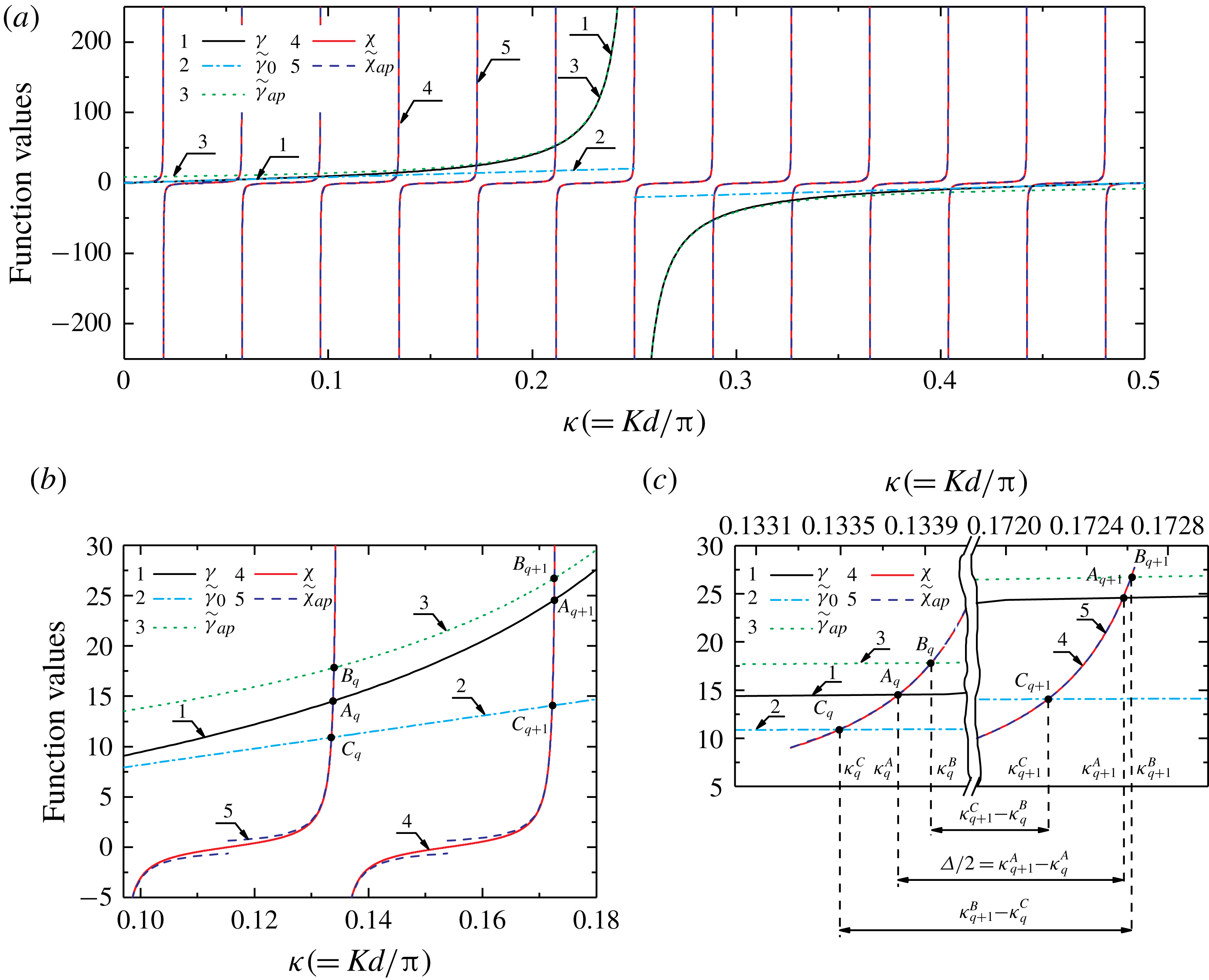
. For example, figure 9(a) shows
 $\unicode[STIX]{x1D6FE}(\unicode[STIX]{x1D705})$
,
 $\unicode[STIX]{x1D712}(\unicode[STIX]{x1D705})$
and their intersections in one period of
 $\unicode[STIX]{x1D6FE}(\unicode[STIX]{x1D705})$
for
 $N=7$
and
 $k=1$
. It is apparent that the intersection points are close to the asymptote of
 $\unicode[STIX]{x1D712}(\unicode[STIX]{x1D705})$
, that is,
 $[4(N-k)+2]\unicode[STIX]{x03C0}\unicode[STIX]{x1D705}=q\unicode[STIX]{x03C0}+\unicode[STIX]{x03C0}/2$
. To obtain the analytical expressions for the abscissae of intersection points, we expand
 $\unicode[STIX]{x1D712}(\unicode[STIX]{x1D705})$
about
 $q\unicode[STIX]{x03C0}+\unicode[STIX]{x03C0}/2$
. Then, near
 $[4(N-k)+2]\unicode[STIX]{x03C0}\unicode[STIX]{x1D705}=q\unicode[STIX]{x03C0}+\unicode[STIX]{x03C0}/2~(q=0,1,2,\ldots )$
, we get
 $$\begin{eqnarray}\tan \{[4(N-k)+2]\unicode[STIX]{x03C0}\unicode[STIX]{x1D705}\}\approx \widetilde{\unicode[STIX]{x1D712}}_{ap}(\unicode[STIX]{x1D705})=\frac{1}{(q\unicode[STIX]{x03C0}+\unicode[STIX]{x03C0}/2)-[4(N-k)+2]\unicode[STIX]{x03C0}\unicode[STIX]{x1D705}}.\end{eqnarray}$$
The notation
 $\widetilde{\unicode[STIX]{x1D712}}_{ap}(\unicode[STIX]{x1D705})$
denotes the expansion of
 $\unicode[STIX]{x1D712}(\unicode[STIX]{x1D705})$
near
 $q\unicode[STIX]{x03C0}+\unicode[STIX]{x03C0}/2$
. Second, we expand
 $\unicode[STIX]{x1D6FE}(\unicode[STIX]{x1D705})=[2(N-k)+1]\tan (2\unicode[STIX]{x03C0}\unicode[STIX]{x1D705})$
about
 $p\unicode[STIX]{x03C0}+\unicode[STIX]{x03C0}/2$
and
 $p\unicode[STIX]{x03C0}~(p=0,1,2,\ldots )$
. Then, near
 $2\unicode[STIX]{x03C0}\unicode[STIX]{x1D705}=p\unicode[STIX]{x03C0}+\unicode[STIX]{x03C0}/2~(p=0,1,2,\ldots )$
, we get
 $$\begin{eqnarray}[2(N-k)+1]\tan (2\unicode[STIX]{x03C0}\unicode[STIX]{x1D705})\approx \widetilde{\unicode[STIX]{x1D6FE}}_{ap}(\unicode[STIX]{x1D705})=\frac{2(N-k)+1}{(p\unicode[STIX]{x03C0}+\unicode[STIX]{x03C0}/2)-2\unicode[STIX]{x03C0}\unicode[STIX]{x1D705}}.\end{eqnarray}$$
Near
 $2\unicode[STIX]{x03C0}\unicode[STIX]{x1D705}=p\unicode[STIX]{x03C0}~(p=0,1,2,\ldots )$
, we get
 $$\begin{eqnarray}[2(N-k)+1]\tan (2\unicode[STIX]{x03C0}\unicode[STIX]{x1D705})\approx \widetilde{\unicode[STIX]{x1D6FE}}_{0}(\unicode[STIX]{x1D705})=\left[2(N-k)+1\right](2\unicode[STIX]{x03C0}\unicode[STIX]{x1D705}-p\unicode[STIX]{x03C0}).\end{eqnarray}$$
For brevity, two notations
 $\widetilde{\unicode[STIX]{x1D6FE}}_{ap}(\unicode[STIX]{x1D705})$
and
 $\widetilde{\unicode[STIX]{x1D6FE}}_{0}(\unicode[STIX]{x1D705})$
are introduced to denote the expansion of
 $\unicode[STIX]{x1D6FE}(\unicode[STIX]{x1D705})$
near
 $p\unicode[STIX]{x03C0}+\unicode[STIX]{x03C0}/2$
and
 $p\unicode[STIX]{x03C0}$
, respectively.
(a) Schematic diagram of
 $\unicode[STIX]{x1D6FE}(\unicode[STIX]{x1D705})$
,
 $\unicode[STIX]{x1D712}(\unicode[STIX]{x1D705})$
and their multiple intersections in interval
 $2\unicode[STIX]{x03C0}\unicode[STIX]{x1D705}\in [0,\unicode[STIX]{x03C0}]$
. (b) Partially enlarged view of upper branches of (a). (c) Partially enlarged view of (b).

Let
 $A_{q}$
be the
 $q$
th intersection point of
 $\unicode[STIX]{x1D6FE}(\unicode[STIX]{x1D705})$
and
 $\unicode[STIX]{x1D712}(\unicode[STIX]{x1D705})$
,
 $B_{q}$
the
 $q$
th intersection point of
 $\widetilde{\unicode[STIX]{x1D6FE}}_{ap}(\unicode[STIX]{x1D705})$
and
 $\unicode[STIX]{x1D712}(\unicode[STIX]{x1D705})$
,
 $C_{q}$
the
 $q$
th intersection point of
 $\widetilde{\unicode[STIX]{x1D6FE}}_{0}(\unicode[STIX]{x1D705})$
and
 $\unicode[STIX]{x1D712}(\unicode[STIX]{x1D705})$
. Point
 $A_{q}$
can also be regarded as the
 $q$
th intersection point of
 $\unicode[STIX]{x1D6FE}(\unicode[STIX]{x1D705})$
and
 $\widetilde{\unicode[STIX]{x1D712}}_{ap}(\unicode[STIX]{x1D705})$
because
 $\widetilde{\unicode[STIX]{x1D712}}_{ap}(\unicode[STIX]{x1D705})$
and
 $\unicode[STIX]{x1D712}(\unicode[STIX]{x1D705})$
are almost completely coincident near
 $A_{q}$
. For
 $B_{q}$
and
 $C_{q}$
, the situations are the same. The intersection points with
 $\unicode[STIX]{x1D712}(\unicode[STIX]{x1D705})$
can be regarded as the intersection points with
 $\widetilde{\unicode[STIX]{x1D712}}_{ap}(\unicode[STIX]{x1D705})$
. Notations
 $\unicode[STIX]{x1D705}_{q}^{A},\unicode[STIX]{x1D705}_{q}^{B}$
and
 $\unicode[STIX]{x1D705}_{q}^{C}$
are the abscissae of
 $A_{q}$
,
 $B_{q}$
and
 $C_{q}$
. These notations are illustrated in figure 9(b,c) taking the upper branches as examples. The difference in ordinates between
 $A_{q}$
and
 $B_{q}$
(or between
 $A_{q}$
and
 $C_{q}$
) may be large if
 $2\unicode[STIX]{x03C0}\unicode[STIX]{x1D705}$
is not close to
 $p\unicode[STIX]{x03C0}+\unicode[STIX]{x03C0}/2$
(or
 $p\unicode[STIX]{x03C0}$
). The difference in abscissae between
 $A_{q}$
and
 $B_{q}$
(
 $C_{q}$
), however, is small because the intersection points are close to the asymptote of
 $\unicode[STIX]{x1D712}(\unicode[STIX]{x1D705})$
, where the derivative values are very large. In other words, we can study
 $\unicode[STIX]{x1D705}_{q}^{B}$
and
 $\unicode[STIX]{x1D705}_{q}^{C}$
first if
 $\unicode[STIX]{x1D705}_{q}^{A}$
is sought. Point
 $A_{q}$
lies between
 $B_{q}$
and
 $C_{q}$
because
 $|\widetilde{\unicode[STIX]{x1D6FE}}_{ap}(\unicode[STIX]{x1D705})|>|\unicode[STIX]{x1D6FE}(\unicode[STIX]{x1D705})|>|\widetilde{\unicode[STIX]{x1D6FE}}_{0}(\unicode[STIX]{x1D705})|$
. Therefore,
 $\unicode[STIX]{x1D705}_{q}^{B}>\unicode[STIX]{x1D705}_{q}^{A}>\unicode[STIX]{x1D705}_{q}^{C}$
(or
 $\unicode[STIX]{x1D705}_{q}^{C}>\unicode[STIX]{x1D705}_{q}^{A}>\unicode[STIX]{x1D705}_{q}^{B}$
for the other branch). The upper and lower bounds of
 $\unicode[STIX]{x1D705}_{q}^{A}$
can be obtained if we get the values of
 $\unicode[STIX]{x1D705}_{q}^{B}$
and
 $\unicode[STIX]{x1D705}_{q}^{C}$
.
Substituting (3.26) and (3.27) into (3.25), we get
 $$\begin{eqnarray}\frac{1}{(q\unicode[STIX]{x03C0}+\unicode[STIX]{x03C0}/2)-\left[4(N-k)+2\right]\unicode[STIX]{x03C0}\unicode[STIX]{x1D705}}=\frac{2(N-k)+1}{(p\unicode[STIX]{x03C0}+\unicode[STIX]{x03C0}/2)-2\unicode[STIX]{x03C0}\unicode[STIX]{x1D705}}.\end{eqnarray}$$
Then,
 $\unicode[STIX]{x1D705}_{q}^{B}$
is obtained by solving (3.29):
 $$\begin{eqnarray}\unicode[STIX]{x1D705}_{q}^{B}=\frac{(q\unicode[STIX]{x03C0}+\unicode[STIX]{x03C0}/2)[2(N-k)+1]-(p\unicode[STIX]{x03C0}+\unicode[STIX]{x03C0}/2)}{2[2(N-k)+1]^{2}\unicode[STIX]{x03C0}-2\unicode[STIX]{x03C0}}.\end{eqnarray}$$
Similarly, by substituting (3.26) and (3.28) into (3.25) and solving the equation, the following real solution is obtained if
 $\unicode[STIX]{x1D705}\neq p/2$
:
 $$\begin{eqnarray}\unicode[STIX]{x1D705}_{q}^{C}=\frac{(q\unicode[STIX]{x03C0}+\unicode[STIX]{x03C0}/2)+p\unicode[STIX]{x03C0}[2(N-k)+1]+\sqrt{\left\{(q\unicode[STIX]{x03C0}+\unicode[STIX]{x03C0}/2)-p\unicode[STIX]{x03C0}[2(N-k)+1]\right\}^{2}-4}}{4[2(N-k)+1]\unicode[STIX]{x03C0}}.\end{eqnarray}$$
Because
 $\unicode[STIX]{x1D705}=p/2$
and its neighbourhood belong to Regions I and II but not to Region III, expression (3.31) can be applied to all of Region III. Here
 $\unicode[STIX]{x1D705}_{q}^{B}$
and
 $\unicode[STIX]{x1D705}_{q}^{C}$
given by (3.30) and (3.31), respectively, are the upper and lower bounds of
 $\unicode[STIX]{x1D705}_{q}^{A}$
, which denotes the abscissa values of the
 $q$
th extreme point (local maximum or minimum point) of
 $\unicode[STIX]{x1D70F}(\unicode[STIX]{x1D705})$
.
Without loss of generality, considering the upper branches, as shown in figure 9(c) (i.e.
 $\unicode[STIX]{x1D705}_{q}^{B}>\unicode[STIX]{x1D705}_{q}^{A}>\unicode[STIX]{x1D705}_{q}^{C}$
), it is apparent that
 $$\begin{eqnarray}\unicode[STIX]{x1D705}_{q+1}^{B}-\unicode[STIX]{x1D705}_{q}^{C}\geqslant \unicode[STIX]{x1D705}_{q+1}^{A}-\unicode[STIX]{x1D705}_{q}^{A}\geqslant \unicode[STIX]{x1D705}_{q+1}^{C}-\unicode[STIX]{x1D705}_{q}^{B}.\end{eqnarray}$$
Using formulae (3.30) and (3.31), and omitting small quantities, we get
 $$\begin{eqnarray}\unicode[STIX]{x1D705}_{q+1}^{B}-\unicode[STIX]{x1D705}_{q}^{C}=\frac{[2(N-k)+1]-(p+1/2)}{2[2(N-k)+1]^{2}}.\end{eqnarray}$$
For the wavenumber range of interest in this study,
 $p$
is not large. For instance,
 $p\leqslant 6$
if
 $\unicode[STIX]{x1D705}\leqslant 3$
. Equation (3.33) can be simplified to
 $$\begin{eqnarray}\unicode[STIX]{x1D705}_{q+1}^{B}-\unicode[STIX]{x1D705}_{q}^{C}=\frac{1}{2[2(N-k)+1]}.\end{eqnarray}$$
Similarly, we can obtain
 $$\begin{eqnarray}\unicode[STIX]{x1D705}_{q+1}^{C}-\unicode[STIX]{x1D705}_{q}^{B}=\frac{1}{2[2(N-k)+1]}.\end{eqnarray}$$
According to (3.32), (3.34) and (3.35),
 $$\begin{eqnarray}\unicode[STIX]{x1D705}_{q+1}^{A}-\unicode[STIX]{x1D705}_{q}^{A}=\frac{1}{2[2(N-k)+1]}.\end{eqnarray}$$
Therefore, the formula for predicting the fluctuation spacing
 $\unicode[STIX]{x1D6E5}$
(the horizontal distance between two adjacent local maximum/minimum points) can be obtained as
 $$\begin{eqnarray}\unicode[STIX]{x1D6E5}_{0}^{N,k}=2(\unicode[STIX]{x1D705}_{q+1}^{A}-\unicode[STIX]{x1D705}_{q}^{A})=\frac{1}{2(N-k)+1}.\end{eqnarray}$$
Here,
 $\unicode[STIX]{x1D6E5}_{0}^{N,k}$
is introduced to denote the fluctuation spacing
 $\unicode[STIX]{x1D6E5}$
of the
 $k$
th cylinder in an array of
 $N$
cylinders in head waves.
3.2.2 Verification
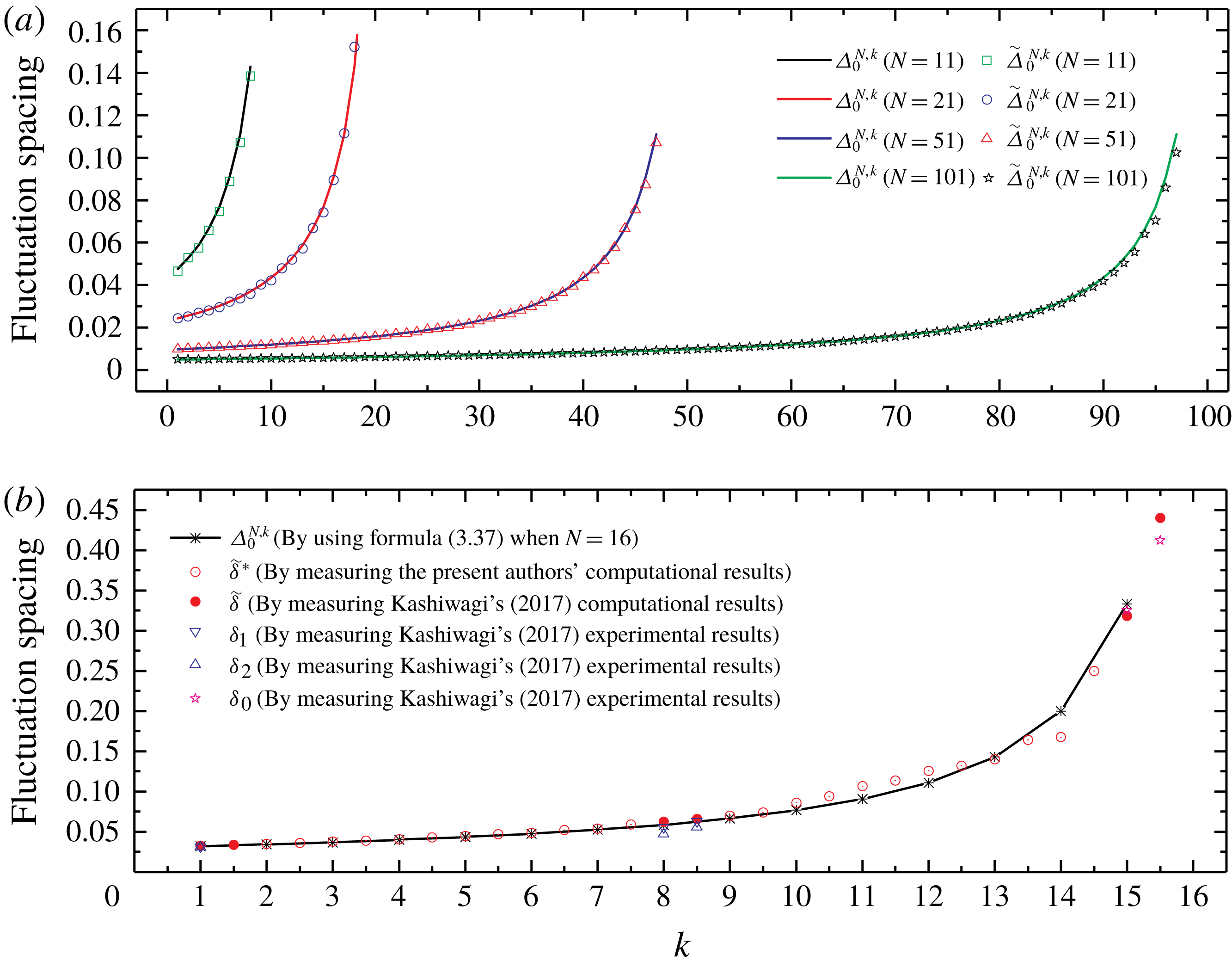
To verify formula (3.37), first, a large number of calculations were performed to determine the wave load based on the interaction theory of Linton & Evans (Reference Linton and Evans1990). Then, we obtained the fluctuation spacing of the magnitude of wave load by measuring the numerical results of the wave load (i.e.
 $\widetilde{\unicode[STIX]{x1D6E5}}_{0}^{N,k}$
). Thereafter, we obtained the fluctuation spacing using formula (3.37) (i.e.
 $\unicode[STIX]{x1D6E5}_{0}^{N,k}$
). Finally, we compared the measured value
 $\widetilde{\unicode[STIX]{x1D6E5}}_{0}^{N,k}$
with the predicted value
 $\unicode[STIX]{x1D6E5}_{0}^{N,k}$
. Most results of
 $\widetilde{\unicode[STIX]{x1D6E5}}_{0}^{N,k}$
and
 $\unicode[STIX]{x1D6E5}_{0}^{N,k}$
show good agreement. In all the cases we calculated, for most cylinders in the array (
 $N-k\geqslant 4$
), the errors are smaller than 2 %. Only for the last few cylinders (
 $N-k\leqslant 4$
) are the errors noticeable (
 ${\sim}5\,\%$
), and the maximum error is smaller than 10 %. These comparisons verify formula (3.37). The formula is very accurate for most cylinders. A few examples involving arrays consisting of 11, 21, 51 or 101 cylinders are shown in figure 10(a).
(a) Comparisons of measured value
 $\widetilde{\unicode[STIX]{x1D6E5}}_{0}^{N,k}$
with predicted value
 $\unicode[STIX]{x1D6E5}_{0}^{N,k}$
given by formula (3.37) for arrays consisting of 11, 21, 51 or 101 cylinders in head waves (
 $\unicode[STIX]{x1D6FD}=0$
). The diameter-to-spacing ratio
 $a/d=1/4$
. (b) Comparisons of the results given by formula (3.37) with the experimental and computational results of a cylinder array of another arrangement (
 $16\times 4$
array of truncated cylinders).

We also verified formula (3.37) by the experimental and computational results of a cylinder array of another arrangement. In figure 5 of Kashiwagi (Reference Kashiwagi2017), the magnitudes of wave elevation at positions along the centreline of
 $16\times 4$
truncated cylinder arrays are shown both numerically and experimentally, and the fact that fluctuation spacing in the curve of wave elevation depends on the position can be observed. We obtained the fluctuation spacings
 $\widetilde{\unicode[STIX]{x1D6FF}}$
,
 $\unicode[STIX]{x1D6FF}_{1}$
,
 $\unicode[STIX]{x1D6FF}_{2}$
and
 $\unicode[STIX]{x1D6FF}_{0}$
in Region III by measuring the computational and experimental results in figure 5 of Kashiwagi (Reference Kashiwagi2017). Spacing
 $\widetilde{\unicode[STIX]{x1D6FF}}$
is the value obtained by measuring the computational results. Spacings
 $\unicode[STIX]{x1D6FF}_{1}$
and
 $\unicode[STIX]{x1D6FF}_{2}$
are the maximum and minimum fluctuation spacings obtained by measuring the experimental results, respectively. The fluctuation spacing is large for downstream positions of the cylinder array. Therefore, it is evident that only half-spacing (i.e. the horizontal spacing between adjacent local maximum point and minimum point) can be measured in the eighth (no. 15) and ninth (between no. 15 and no. 16) graphs in figure 5 of Kashiwagi (Reference Kashiwagi2017). In order to facilitate subsequent comparisons, we multiplied the half-spacing by 2 to indicate the fluctuation spacing. For these cases, only one fluctuation spacing
 $\unicode[STIX]{x1D6FF}_{0}$
can be obtained by measuring the experimental results. For the positions on the centreline where the results of wave amplitude are not given in figure 5 of Kashiwagi (Reference Kashiwagi2017), we calculated the wave elevation based on interaction theory of Kagemoto & Yue (Reference Kagemoto and Yue1986) and measured the fluctuation spacing
 $\widetilde{\unicode[STIX]{x1D6FF}}^{\ast }$
. Thereafter we obtained
 $\unicode[STIX]{x1D6E5}_{0}^{N,k}$
by substituting
 $N=16$
into formula (3.37). Spacings
 $\widetilde{\unicode[STIX]{x1D6FF}}$
,
 $\widetilde{\unicode[STIX]{x1D6FF}}^{\ast }$
,
 $\unicode[STIX]{x1D6FF}_{1}$
,
 $\unicode[STIX]{x1D6FF}_{2}$
and
 $\unicode[STIX]{x1D6FF}_{0}$
are the fluctuation spacings of wave amplitude, while
 $\unicode[STIX]{x1D6E5}_{0}^{N,k}$
is the fluctuation spacing of magnitude of wave loads. In addition,
 $\widetilde{\unicode[STIX]{x1D6FF}}$
,
 $\widetilde{\unicode[STIX]{x1D6FF}}^{\ast }$
,
 $\unicode[STIX]{x1D6FF}_{1}$
,
 $\unicode[STIX]{x1D6FF}_{2}$
and
 $\unicode[STIX]{x1D6FF}_{0}$
are the results at positions on the centreline of a
 $16\times 4$
array of truncated cylinders, while
 $\unicode[STIX]{x1D6E5}_{0}^{N,k}$
is the result for a certain cylinder of a straight-line array of bottom-mounted cylinders. Given these obvious differences, the agreement can be said to be quite good, as shown in figure 10(b).
3.3 Formula for fluctuation spacing in oblique waves
In this subsection, a cylinder array in obliquely incident waves (
 $\unicode[STIX]{x1D6FD}\neq 0$
) is discussed, which is more complex than the situation of a cylinder array in head waves (
 $\unicode[STIX]{x1D6FD}=0$
). It is difficult to obtain the formula of fluctuation spacing for
 $\unicode[STIX]{x1D6FD}\neq 0$
by following the same method as that for
 $\unicode[STIX]{x1D6FD}=0$
, which was presented in § 3.2. However, the work on
 $\unicode[STIX]{x1D6FD}=0$
presents significant insights that can be applied to the situation in which
 $\unicode[STIX]{x1D6FD}\neq 0$
. The analysis of
 ${\mathcal{D}}_{n}^{k}(\unicode[STIX]{x1D705})$
for
 $\unicode[STIX]{x1D6FD}=0$
in § 3.2 helped us consider
 ${\mathcal{D}}_{n}^{k}(\unicode[STIX]{x1D705})$
for
 $\unicode[STIX]{x1D6FD}\neq 0$
.
According to (3.11)–(3.13), for
 $\unicode[STIX]{x1D6FD}\neq 0$
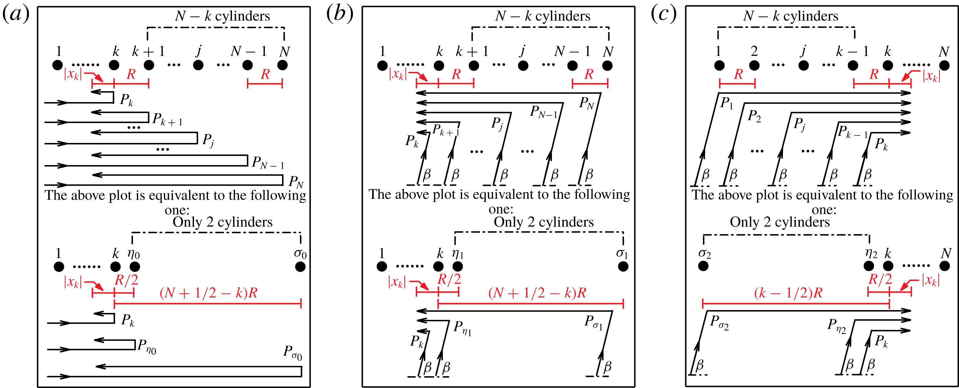
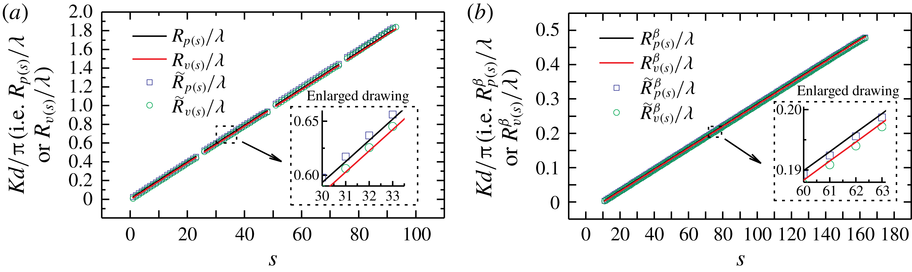
,
 $$\begin{eqnarray}{\mathcal{D}}_{n}^{k}(\unicode[STIX]{x1D705})=\unicode[STIX]{x1D709}(\unicode[STIX]{x1D705})-\unicode[STIX]{x1D709}_{1}^{0}(\unicode[STIX]{x1D705})\unicode[STIX]{x1D6EC}_{1}^{0}(\unicode[STIX]{x1D705})+\unicode[STIX]{x1D709}_{2}^{0}(\unicode[STIX]{x1D705})\unicode[STIX]{x1D6EC}_{2}^{0}(\unicode[STIX]{x1D705})-\unicode[STIX]{x1D709}_{1}^{\unicode[STIX]{x03C0}}(\unicode[STIX]{x1D705})\unicode[STIX]{x1D6EC}_{1}^{\unicode[STIX]{x03C0}}(\unicode[STIX]{x1D705})+\unicode[STIX]{x1D709}_{2}^{\unicode[STIX]{x03C0}}(\unicode[STIX]{x1D705})\unicode[STIX]{x1D6EC}_{2}^{\unicode[STIX]{x03C0}}(\unicode[STIX]{x1D705}),\end{eqnarray}$$
where
 $$\begin{eqnarray}\displaystyle & \displaystyle \unicode[STIX]{x1D6EC}_{1}^{0}(\unicode[STIX]{x1D705})=\mathop{\sum }_{j=1}^{k-1}\sqrt{\frac{1}{k-j}}\cos [2\unicode[STIX]{x03C0}\unicode[STIX]{x1D705}(k-j)(1-\cos \unicode[STIX]{x1D6FD})], & \displaystyle\end{eqnarray}$$
 $$\begin{eqnarray}\displaystyle & \displaystyle \unicode[STIX]{x1D6EC}_{2}^{0}(\unicode[STIX]{x1D705})=\mathop{\sum }_{j=1}^{k-1}\sqrt{\frac{1}{k-j}}\sin [2\unicode[STIX]{x03C0}\unicode[STIX]{x1D705}(k-j)(1-\cos \unicode[STIX]{x1D6FD})], & \displaystyle\end{eqnarray}$$
 $$\begin{eqnarray}\displaystyle & \displaystyle \unicode[STIX]{x1D6EC}_{1}^{\unicode[STIX]{x03C0}}(\unicode[STIX]{x1D705})=\mathop{\sum }_{j=k+1}^{N}\sqrt{\frac{1}{j-k}}\cos [2\unicode[STIX]{x03C0}\unicode[STIX]{x1D705}(j-k)(1+\cos \unicode[STIX]{x1D6FD})], & \displaystyle\end{eqnarray}$$
 $$\begin{eqnarray}\displaystyle & \displaystyle \unicode[STIX]{x1D6EC}_{2}^{\unicode[STIX]{x03C0}}(\unicode[STIX]{x1D705})=\mathop{\sum }_{j=k+1}^{N}\sqrt{\frac{1}{j-k}}\sin [2\unicode[STIX]{x03C0}\unicode[STIX]{x1D705}(j-k)(1+\cos \unicode[STIX]{x1D6FD})]. & \displaystyle\end{eqnarray}$$
Here
 $\unicode[STIX]{x1D709}_{1}^{0}(\unicode[STIX]{x1D705})\unicode[STIX]{x1D6EC}_{1}^{0}(\unicode[STIX]{x1D705})$
and
 $\unicode[STIX]{x1D709}_{2}^{0}(\unicode[STIX]{x1D705})\unicode[STIX]{x1D6EC}_{2}^{0}(\unicode[STIX]{x1D705})$
are the contributions of the cylinders upstream of cylinder
 $k$
and
 $\unicode[STIX]{x1D709}_{1}^{\unicode[STIX]{x03C0}}(\unicode[STIX]{x1D705})\unicode[STIX]{x1D6EC}_{1}^{\unicode[STIX]{x03C0}}(\unicode[STIX]{x1D705})$
and
 $\unicode[STIX]{x1D709}_{2}^{\unicode[STIX]{x03C0}}(\unicode[STIX]{x1D705})\unicode[STIX]{x1D6EC}_{2}^{\unicode[STIX]{x03C0}}(\unicode[STIX]{x1D705})$
are the contributions of the cylinders downstream of cylinder
 $k$
. In contrast to the situation of
 $\unicode[STIX]{x1D6FD}=0$
, both upstream and downstream cylinders affect
 ${\mathcal{D}}_{n}^{k}(\unicode[STIX]{x1D705})$
when
 $\unicode[STIX]{x1D6FD}\neq 0$
.
Similar to (3.22), based on the product-to-sum identities of trigonometric functions, excluding the cases where the denominators are equal to zero, equations (3.39)–(3.42) can be rewritten as
 $$\begin{eqnarray}\displaystyle & & \displaystyle \unicode[STIX]{x1D6EC}_{1}^{0}(\unicode[STIX]{x1D705})=\frac{1}{2\sin [(1-\cos \unicode[STIX]{x1D6FD})\unicode[STIX]{x03C0}\unicode[STIX]{x1D705}]}\left\{-\sin [(1-\cos \unicode[STIX]{x1D6FD})\unicode[STIX]{x03C0}\unicode[STIX]{x1D705}]+\sqrt{\frac{1}{k-1}}\sin \left[(2(k-1)+1)\right.\right.\nonumber\\ \displaystyle & & \displaystyle \quad \left.\left.\text{}\times (1-\cos \unicode[STIX]{x1D6FD})\unicode[STIX]{x03C0}\unicode[STIX]{x1D705}\right]+\mathop{\sum }_{j=2}^{k-1}\left(\sqrt{\frac{1}{j-1}}-\sqrt{\frac{1}{j}}\right)\sin [(2(j-1)+1)(1-\cos \unicode[STIX]{x1D6FD})\unicode[STIX]{x03C0}\unicode[STIX]{x1D705}]\right\},\nonumber\\ \displaystyle & & \displaystyle\end{eqnarray}$$
 $$\begin{eqnarray}\displaystyle & & \displaystyle \unicode[STIX]{x1D6EC}_{2}^{0}(\unicode[STIX]{x1D705})=\frac{1}{2\sin \left[(1-\cos \unicode[STIX]{x1D6FD})\unicode[STIX]{x03C0}\unicode[STIX]{x1D705}\right]}\left\{\cos \left[(1-\cos \unicode[STIX]{x1D6FD})\unicode[STIX]{x03C0}\unicode[STIX]{x1D705}\right]-\sqrt{\frac{1}{k-1}}\cos \left[\left(2(k-1)+1\right)\right.\right.\nonumber\\ \displaystyle & & \displaystyle \quad \left.\left.\text{}\times (1-\cos \unicode[STIX]{x1D6FD})\unicode[STIX]{x03C0}\unicode[STIX]{x1D705}\right]-\mathop{\sum }_{j=2}^{k-1}\left(\sqrt{\frac{1}{j-1}}-\sqrt{\frac{1}{j}}\right)\cos [(2(j-1)+1)(1-\cos \unicode[STIX]{x1D6FD})\unicode[STIX]{x03C0}\unicode[STIX]{x1D705}]\right\},\nonumber\\ \displaystyle & & \displaystyle\end{eqnarray}$$
 $$\begin{eqnarray}\displaystyle & & \displaystyle \unicode[STIX]{x1D6EC}_{1}^{\unicode[STIX]{x03C0}}(\unicode[STIX]{x1D705})=\frac{1}{2\sin [(1+\cos \unicode[STIX]{x1D6FD})\unicode[STIX]{x03C0}\unicode[STIX]{x1D705}]}\left\{\!-\sin [(1+\cos \unicode[STIX]{x1D6FD})\unicode[STIX]{x03C0}\unicode[STIX]{x1D705}]+\sqrt{\frac{1}{N-k}}\sin \left[(2(N-k)+1)\right.\right.\nonumber\\ \displaystyle & & \displaystyle \quad \left.\left.\text{}\times (1+\cos \unicode[STIX]{x1D6FD})\unicode[STIX]{x03C0}\unicode[STIX]{x1D705}\right]+\mathop{\sum }_{j=2}^{k-1}\left(\sqrt{\frac{1}{j-1}}-\sqrt{\frac{1}{j}}\right)\sin [(2(j-1)+1)(1+\cos \unicode[STIX]{x1D6FD})\unicode[STIX]{x03C0}\unicode[STIX]{x1D705}]\right\},\nonumber\\ \displaystyle & & \displaystyle\end{eqnarray}$$
 $$\begin{eqnarray}\displaystyle & & \displaystyle \unicode[STIX]{x1D6EC}_{2}^{\unicode[STIX]{x03C0}}(\unicode[STIX]{x1D705})=\frac{1}{2\sin \left[(1+\cos \unicode[STIX]{x1D6FD})\unicode[STIX]{x03C0}\unicode[STIX]{x1D705}\right]}\left\{\cos \left[(1+\cos \unicode[STIX]{x1D6FD})\unicode[STIX]{x03C0}\unicode[STIX]{x1D705}\right]-\sqrt{\frac{1}{N-k}}\cos \left[\left(2(N-k)+1\right)\right.\right.\nonumber\\ \displaystyle & & \displaystyle \quad \left.\left.\text{}\times (1+\cos \unicode[STIX]{x1D6FD})\unicode[STIX]{x03C0}\unicode[STIX]{x1D705}\right]-\mathop{\sum }_{j=2}^{k-1}\left(\sqrt{\frac{1}{j-1}}-\sqrt{\frac{1}{j}}\right)\cos [(2(j-1)+1)(1+\cos \unicode[STIX]{x1D6FD})\unicode[STIX]{x03C0}\unicode[STIX]{x1D705}]\right\}.\nonumber\\ \displaystyle & & \displaystyle\end{eqnarray}$$
For reasons similar to those mentioned in the discussion related to formula (3.23), (3.43)–(3.46) can be simplified as
 $$\begin{eqnarray}\unicode[STIX]{x1D6EC}_{1}^{0}(\unicode[STIX]{x1D705})=\frac{-\sin [(1-\cos \unicode[STIX]{x1D6FD})\unicode[STIX]{x03C0}\unicode[STIX]{x1D705}]+\sqrt{{\displaystyle \frac{1}{k-1}}}\sin \{[2(k-1)+1](1-\cos \unicode[STIX]{x1D6FD})\unicode[STIX]{x03C0}\unicode[STIX]{x1D705}\}}{2\sin [(1-\cos \unicode[STIX]{x1D6FD})\unicode[STIX]{x03C0}\unicode[STIX]{x1D705}]},\end{eqnarray}$$
 $$\begin{eqnarray}\displaystyle & \displaystyle \unicode[STIX]{x1D6EC}_{2}^{0}(\unicode[STIX]{x1D705})=\frac{\cos [(1-\cos \unicode[STIX]{x1D6FD})\unicode[STIX]{x03C0}\unicode[STIX]{x1D705}]-\sqrt{{\displaystyle \frac{1}{k-1}}}\cos \{[2(k-1)+1](1-\cos \unicode[STIX]{x1D6FD})\unicode[STIX]{x03C0}\unicode[STIX]{x1D705}\}}{2\sin [(1-\cos \unicode[STIX]{x1D6FD})\unicode[STIX]{x03C0}\unicode[STIX]{x1D705}]}, & \displaystyle \nonumber\\ \displaystyle & & \displaystyle\end{eqnarray}$$
 $$\begin{eqnarray}\displaystyle & \displaystyle \unicode[STIX]{x1D6EC}_{1}^{\unicode[STIX]{x03C0}}(\unicode[STIX]{x1D705})=\frac{-\sin [(1+\cos \unicode[STIX]{x1D6FD})\unicode[STIX]{x03C0}\unicode[STIX]{x1D705}]+\sqrt{{\displaystyle \frac{1}{N-k}}}\sin \{[2(N-k)+1](1+\cos \unicode[STIX]{x1D6FD})\unicode[STIX]{x03C0}\unicode[STIX]{x1D705}\}}{2\sin [(1+\cos \unicode[STIX]{x1D6FD})\unicode[STIX]{x03C0}\unicode[STIX]{x1D705}]}, & \displaystyle \nonumber\\ \displaystyle & & \displaystyle\end{eqnarray}$$
 $$\begin{eqnarray}\displaystyle & \displaystyle \unicode[STIX]{x1D6EC}_{2}^{\unicode[STIX]{x03C0}}(\unicode[STIX]{x1D705})=\frac{\cos [(1+\cos \unicode[STIX]{x1D6FD})\unicode[STIX]{x03C0}\unicode[STIX]{x1D705}]-\sqrt{{\displaystyle \frac{1}{N-k}}}\cos \{[2(N-k)+1](1+\cos \unicode[STIX]{x1D6FD})\unicode[STIX]{x03C0}\unicode[STIX]{x1D705}\}}{2\sin [(1+\cos \unicode[STIX]{x1D6FD})\unicode[STIX]{x03C0}\unicode[STIX]{x1D705}]}. & \displaystyle \nonumber\\ \displaystyle & & \displaystyle\end{eqnarray}$$
Both upstream and downstream cylinders affecting
 ${\mathcal{D}}_{n}^{k}(\unicode[STIX]{x1D705})$
when
 $\unicode[STIX]{x1D6FD}\neq 0$
impede derivation of the formula for fluctuation spacing according to the method presented in § 3.2. Hence, a heuristic approach is adopted in this subsection to obtain the said formula. We derive the formula more rigorously for
 $\unicode[STIX]{x1D6FD}\neq 0$
in the next section based on the constructive/destructive interference of diffraction waves.
The discussions pertaining to
 $\unicode[STIX]{x1D70F}(\unicode[STIX]{x1D705})$
in § 3.2 show that only the contribution of the last cylinder in the array (cylinder
 $N$
) is significant in the situation of
 $\unicode[STIX]{x1D6FD}=0$
. However, after observing (3.47)–(3.50), we realized that both the first cylinder (cylinder 1) and the last cylinder (cylinder
 $N$
) in the array contribute to the fluctuation spacing in the situation of
 $\unicode[STIX]{x1D6FD}\neq 0$
. This was confirmed by our computations.
Our computation indicates three possible scenarios for the curve of magnitude of wave load. (1) Similar to the situation for
 $\unicode[STIX]{x1D6FD}=0$
, there is one obvious constant fluctuation spacing in Region III, which is considerably less than the spacing between two spikes (i.e.
 ${\sim}0.5$
). (2) There are two obvious constant fluctuation spacings in Region III, and both are considerably smaller than 0.5. (3) There seems to be no obvious constant fluctuation spacing in the plot of magnitude of wave load versus
 $Kd/\unicode[STIX]{x03C0}$
curves, but if the curves are analysed using fast Fourier transform (FFT), two distinct peaks close to each other can be observed, suggesting the existence of two constant fluctuation spacings that are considerably smaller than 0.5 in the curve of magnitude of wave load.
The contributions of the first and the last cylinder in the array are different for each
 $N,k$
and
 $\unicode[STIX]{x1D6FD}$
combination. Thus, scenarios (1) and (2) can be further divided into four scenarios. The computations show that scenario (1) can be divided into two sub-scenarios. One is for the case
 $[2(N-k)+1](1+\cos \unicode[STIX]{x1D6FD})\gg [2(k-1)+1](1-\cos \unicode[STIX]{x1D6FD})$
, and the other is for the case
 $[2(k-1)+1](1-\cos \unicode[STIX]{x1D6FD})\gg [2(N-k)+1](1+\cos \unicode[STIX]{x1D6FD})$
. Scenario (2) can be divided into two sub-scenarios as well. One is for the case
 $[2(N-k)+1](1+\cos \unicode[STIX]{x1D6FD})>[2(k-1)+1](1-\cos \unicode[STIX]{x1D6FD})\gg 4$
, and the other is for the case
 $[2(k-1)+1](1-\cos \unicode[STIX]{x1D6FD})>[2(N-k)+1](1+\cos \unicode[STIX]{x1D6FD})\gg 4$
. Therefore, for
 $\unicode[STIX]{x1D6FD}\neq 0$
, we discuss five scenarios.
Scenario 1:
 $[2(N-k)+1](1+\cos \unicode[STIX]{x1D6FD})\gg [2(k-1)+1](1-\cos \unicode[STIX]{x1D6FD})$
. In this scenario,
 $\unicode[STIX]{x1D6EC}_{1}^{0}(\unicode[STIX]{x1D705})$
and
 $\unicode[STIX]{x1D6EC}_{2}^{0}(\unicode[STIX]{x1D705})$
, defined by expressions (3.47) and (3.48), respectively, are slowly varying functions, and
 $\unicode[STIX]{x1D6EC}_{1}^{\unicode[STIX]{x03C0}}(\unicode[STIX]{x1D705})$
and
 $\unicode[STIX]{x1D6EC}_{2}^{\unicode[STIX]{x03C0}}(\unicode[STIX]{x1D705})$
, defined by expressions (3.49) and (3.50), are rapidly oscillating functions. Given our focus on the minimum fluctuation spacing of the wave load, only the terms containing
 $[2(N-k)+1](1+\cos \unicode[STIX]{x1D6FD})$
need to be considered. In other words, it is adequate to consider only the contributions obtained using expressions (3.49) and (3.50). Using a technique similar to that employed in the process of derivation from (3.25) to (3.37), the formula for minimum fluctuation spacing in scenario 1 can be obtained as follows:
 $$\begin{eqnarray}\unicode[STIX]{x1D6E5}_{\unicode[STIX]{x1D6FD},ds}^{N,k}=\frac{2}{[2(N-k)+1](1+\cos \unicode[STIX]{x1D6FD})},\end{eqnarray}$$
where the subscript ‘
 $ds$
’ denotes downstream, showing that only the last cylinder in the array contributes to the fluctuation spacing of cylinder
 $k$
in this scenario.
Figure 11(A) shows an example (
 $N=301,k=15$
and
 $\unicode[STIX]{x1D6FD}=\unicode[STIX]{x03C0}/6$
) of scenario 1, where the fluctuation spacing
 $\unicode[STIX]{x1D6E5}$
can be determined using formula (3.51). The value of fluctuation spacing obtained by measuring the curve in figure 11(A) is
 $\widetilde{\unicode[STIX]{x1D6E5}}_{\unicode[STIX]{x03C0}/6,ds}^{301,15}=0.001868$
. The corresponding value obtained using the prediction formula (3.51) is
 $\unicode[STIX]{x1D6E5}_{\unicode[STIX]{x03C0}/6,ds}^{301,15}=0.001870$
. Figure 11(a) shows the result of FFT analysis of figure 11(A), which indicates that the fluctuation spacing is
 $\bar{\unicode[STIX]{x1D6E5}}_{\unicode[STIX]{x03C0}/6,ds}^{301,15}=0.001865$
. Hence, the theoretical value
 $\unicode[STIX]{x1D6E5}_{\unicode[STIX]{x03C0}/6,ds}^{301,15}$
agrees well with
 $\widetilde{\unicode[STIX]{x1D6E5}}_{\unicode[STIX]{x03C0}/6,ds}^{301,15}$
and
 $\bar{\unicode[STIX]{x1D6E5}}_{\unicode[STIX]{x03C0}/6,ds}^{301,15}$
.
Scenario 2:
 $[2(k-1)+1](1-\cos \unicode[STIX]{x1D6FD})\gg [2(N-k)+1](1+\cos \unicode[STIX]{x1D6FD})$
. In this scenario,
 $\unicode[STIX]{x1D6EC}_{1}^{0}(\unicode[STIX]{x1D705})$
and
 $\unicode[STIX]{x1D6EC}_{2}^{0}(\unicode[STIX]{x1D705})$
are rapidly oscillating functions, and
 $\unicode[STIX]{x1D6EC}_{1}^{\unicode[STIX]{x03C0}}(\unicode[STIX]{x1D705})$
and
 $\unicode[STIX]{x1D6EC}_{2}^{\unicode[STIX]{x03C0}}(\unicode[STIX]{x1D705})$
are slowly varying functions. Thus, only the terms containing
 $[2(k-1)+1](1-\cos \unicode[STIX]{x1D6FD})$
need to be considered. Similar to the discussion for scenario 1, the formula for the minimum fluctuation spacing in scenario 2 is
 $$\begin{eqnarray}\unicode[STIX]{x1D6E5}_{\unicode[STIX]{x1D6FD},us}^{N,k}=\frac{2}{[2(k-1)+1](1-\cos \unicode[STIX]{x1D6FD})},\end{eqnarray}$$
where the subscript ‘
 $us$
’ denotes upstream, indicating that only the first cylinder in the array contributes to the fluctuation spacing of cylinder
 $k$
in this scenario.
Similar to scenario 1, we show an example (
 $N=301,k=299$
and
 $\unicode[STIX]{x1D6FD}=4\unicode[STIX]{x03C0}/9$
) of scenario 2 in figure 11(B,b). The three results of fluctuation spacing (
 $\unicode[STIX]{x1D6E5}_{\unicode[STIX]{x1D6FD},us}^{N,k}$
,
 $\widetilde{\unicode[STIX]{x1D6E5}}_{\unicode[STIX]{x1D6FD},us}^{N,k}$
,
 $\bar{\unicode[STIX]{x1D6E5}}_{\unicode[STIX]{x1D6FD},us}^{N,k}$
) obtained using formula (3.52), measuring the curve in figure 11(B), and performing FFT analysis on the curve are shown in table 1. They are in good agreement.
Five scenarios of the curve of magnitude of wave load on the
 $k$
th cylinder (A–E) and the corresponding results of FFT analysis (a–e). Here
 $N=301$
and
 $a/d=1/4$
.
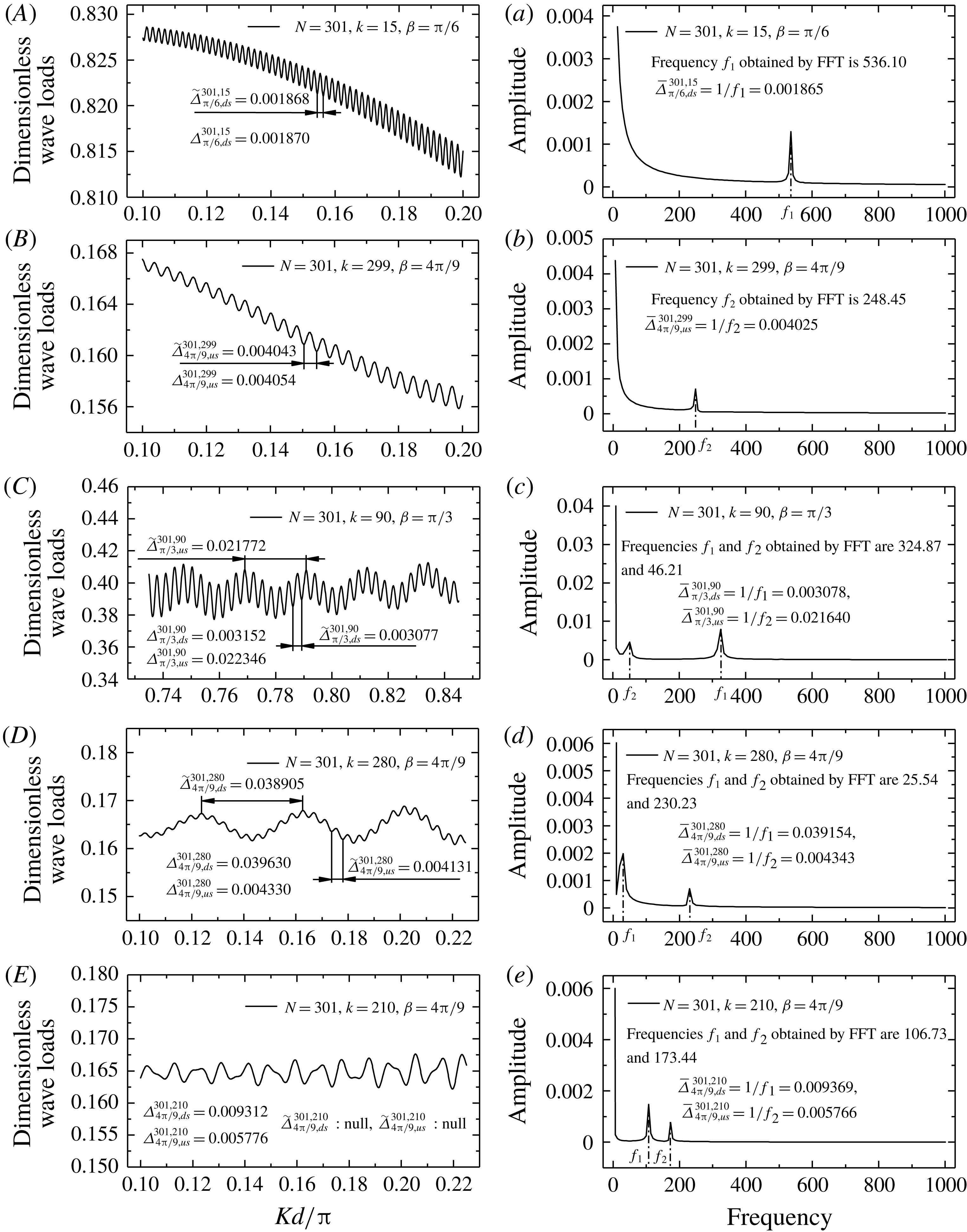
Examples for different scenarios when
 $\unicode[STIX]{x1D6FD}\neq 0$
. The fluctuation spacings shown here are 1000 times the real values. Spacings
 $\unicode[STIX]{x1D6E5}_{\unicode[STIX]{x1D6FD},ds}^{N,k}$
and
 $\unicode[STIX]{x1D6E5}_{\unicode[STIX]{x1D6FD},us}^{N,k}$
are obtained using formulae (3.51) and (3.52). Spacings
 $\widetilde{\unicode[STIX]{x1D6E5}}_{\unicode[STIX]{x1D6FD},ds}^{N,k}$
and
 $\widetilde{\unicode[STIX]{x1D6E5}}_{\unicode[STIX]{x1D6FD},us}^{N,k}$
are obtained by measuring curves in figure 11(A–D). Spacings
 $\bar{\unicode[STIX]{x1D6E5}}_{\unicode[STIX]{x1D6FD},ds}^{N,k}$
and
 $\bar{\unicode[STIX]{x1D6E5}}_{\unicode[STIX]{x1D6FD},us}^{N,k}$
are obtained using results of FFT analysis for figure 11(A–E), as shown in figure 11(a–e).

Our computations show that the majority of the cases we calculated can be categorized as scenarios 1 and 2, and most of them can be categorized as scenario 1. For the other small numbers of cases, there are two (or there seems even no) constant fluctuation spacings in Region III. Scenarios 1 and 2 are two simple scenarios. For other scenarios, it is difficult to obtain the formula using the same technique. Equations (3.38) and (3.47)–(3.50) show that
 ${\mathcal{D}}_{n}^{k}(\unicode[STIX]{x1D705})$
is superposed by multiple trigonometric functions with slowly varying amplitudes. Then, it can be inferred that for scenarios other than scenarios 1 and 2, the fluctuation spacing in Region III can possibly be determined using (3.51) and (3.52). The difference is that the value should be calculated first using (3.51) and (3.52), and the smaller value should be taken as the minimum fluctuation spacing. By FFT analysis, we confirmed that in each scenario, the smaller of the values obtained using formulas (3.51) and (3.52) can be considered the minimum fluctuation spacing.
Scenario 3:
 $[2(N-k)+1](1+\cos \unicode[STIX]{x1D6FD})>[2(k-1)+1](1-\cos \unicode[STIX]{x1D6FD})\gg 4$
. In this scenario, although
 $\unicode[STIX]{x1D6EC}_{1}^{0}(\unicode[STIX]{x1D705})$
and
 $\unicode[STIX]{x1D6EC}_{2}^{0}(\unicode[STIX]{x1D705})$
oscillate more slowly than
 $\unicode[STIX]{x1D6EC}_{1}^{\unicode[STIX]{x03C0}}(\unicode[STIX]{x1D705})$
and
 $\unicode[STIX]{x1D6EC}_{2}^{\unicode[STIX]{x03C0}}(\unicode[STIX]{x1D705})$
,
 $[2(k-1)+1](1-\cos \unicode[STIX]{x1D6FD})\gg 4$
implies that the fluctuation spacing given by formula (3.52) is considerably smaller than the spacing between two adjacent spikes (multiple Regions III are separated by several spikes, where the spacing between two adjacent spikes is about 0.5). Hence, there are two distinct fluctuation spacings in Region III, where the smaller value is given by (3.51) and the larger value by (3.52). The minimum fluctuation spacing is the smaller value, which can be predicted using (3.51). An example (
 $N=301,k=90$
and
 $\unicode[STIX]{x1D6FD}=\unicode[STIX]{x03C0}/3$
) is shown in figure 11(C,c) and table 1 for scenario 3.
Scenario 4:
 $[2(k-1)+1](1-\cos \unicode[STIX]{x1D6FD})>[2(N-k)+1](1+\cos \unicode[STIX]{x1D6FD})\gg 4$
. This scenario is similar to scenario 3. There are two distinct fluctuation spacings in Region III, where the smaller spacing is given by (3.52) and the larger spacing by (3.51). The minimum fluctuation spacing is the smaller value, which can be predicted using formula (3.52). An example (
 $N=301,k=280$
and
 $\unicode[STIX]{x1D6FD}=4\unicode[STIX]{x03C0}/9$
) is shown in figure 11(D,d) and table 1 for scenario 4.
Scenario 5:
 $[2(N-k)+1](1+\cos \unicode[STIX]{x1D6FD})$
and
 $[2(k-1)+1](1-\cos \unicode[STIX]{x1D6FD})$
are of the same order of magnitude and are significantly greater than 4. This scenario is rare. In this scenario, the differences between the fluctuation characteristics of
 $\unicode[STIX]{x1D6EC}_{1}^{0}(\unicode[STIX]{x1D705})~(\unicode[STIX]{x1D6EC}_{2}^{0}(\unicode[STIX]{x1D705}))$
and
 $\unicode[STIX]{x1D6EC}_{1}^{\unicode[STIX]{x03C0}}(\unicode[STIX]{x1D705})~(\unicode[STIX]{x1D6EC}_{2}^{\unicode[STIX]{x03C0}}(\unicode[STIX]{x1D705}))$
are not large. Thus, the superposition of these functions no longer exhibits distinct regular fluctuation. It seems that the rules valid for scenarios 1–4 no longer apply to this scenario. It is difficult to identify clear fluctuation spacings directly from the curve of magnitude of wave load. However, FFT analysis will yield results similar to those obtained in scenarios 3 and 4. This suggests that the intrinsic mechanism for the irregular appearance of the curve of magnitude of wave load in scenario 5 is identical to those of scenarios 3 and 4. The fluctuation spacing in this scenario is redefined as the reciprocal of the frequency corresponding to the peaks in the results curve of FFT analysis. Such fluctuation spacing can still be predicted using formulae (3.51) and (3.52) if the results of FFT analysis are considered instead of the corresponding curves of magnitude of wave load. An example (
 $N=301,k=210$
and
 $\unicode[STIX]{x1D6FD}=4\unicode[STIX]{x03C0}/9$
) is shown in figure 11(E,e) and table 1 for scenario 5.


In fact, the differences in appearance among the curves of magnitude of wave load in all five scenarios are caused only by the relative size of
 $[2(N-k)+1](1+\cos \unicode[STIX]{x1D6FD})$
and
 $[2(k-1)+1](1-\cos \unicode[STIX]{x1D6FD})$
. In other words, the differences in appearance stem from the differences in the contributions of the last cylinder and the first cylinder in the array. Our computations show that scenario 1 is the most frequently encountered scenario, while scenario 5 is the least frequently encountered scenario. This suggests that the contribution of the last cylinder in the array is significant in most of the cases, and the contribution of the first cylinder is manifested in a few of the cases. Therefore, occasionally, there are two distinct fluctuation spacings in Region III for
 $\unicode[STIX]{x1D6FD}\neq 0$
. The smaller one is termed the minimum fluctuation spacing. It should be noted that for
 $\unicode[STIX]{x1D6FD}=0$
, as mentioned in § 3.2, only the contributions of the last cylinder are significant. There is only one fluctuation spacing, which is considerably smaller than the spacing between two adjacent spikes (
 ${\sim}0.5$
). In other words, there is only one scenario for
 $\unicode[STIX]{x1D6FD}=0$
, which is similar to scenario 1 for
 $\unicode[STIX]{x1D6FD}\neq 0$
.
Considering the discussions of all scenarios and synthesizing formulae (3.51) and (3.52), the minimum fluctuation spacing in Region III for
 $\unicode[STIX]{x1D6FD}\neq 0$
can be determined using the following formula:
 $$\begin{eqnarray}\unicode[STIX]{x1D6E5}_{\unicode[STIX]{x1D6FD}}^{N,k}=\text{min}\left\{\frac{2}{[2(N-k)+1](1+\cos \unicode[STIX]{x1D6FD})},\frac{2}{[2(k-1)+1](1-\cos \unicode[STIX]{x1D6FD})}\right\}.\end{eqnarray}$$
An example (
 $N=301$
) of the fluctuation spacing obtained using formulae (3.51) and (3.52) is shown in figure 12. The orange surface denotes the contributions of the last cylinder in the array, and the cyan surface denotes the contribution of the first cylinder in the array. In the majority of the cases, the orange surface is under the cyan surface.
4 Derivation of formulae for fluctuation spacings based on constructive/destructive interference and understanding of physical mechanism
In this section, we consider the constructive/destructive interference of waves. Then, we derive the formulae for predicting fluctuation spacings and reveal the underlying physical mechanism. Wave interference is encountered widely in many domains, for instance Young’s double-slit interference experiment for light waves in optics and Bragg diffraction in solid-state physics when X-rays are incident on the atoms of a crystalline system. When the diffraction waves interfere constructively (or destructively), the phase difference between the two waves is equal to an integer multiple of
 $2\unicode[STIX]{x03C0}$
(or odd multiple of
 $\unicode[STIX]{x03C0}$
), and the difference in path lengths between the two waves is an integer multiple of the wavelength (or odd multiple of half-wavelength); and vice versa.
4.1 Formula for the fluctuation spacing in head waves
In this subsection, we consider the constructive/destructive interference of diffracted waves for arrays of cylinders in head waves (
 $\unicode[STIX]{x1D6FD}=0$
). We rewrite
 $Kd/\unicode[STIX]{x03C0}$
as follows:
 $$\begin{eqnarray}\frac{Kd}{\unicode[STIX]{x03C0}}=\frac{R}{\unicode[STIX]{x1D706}},\end{eqnarray}$$
where
 $R=2d$
is the spacing between adjacent cylinders, and
 $\unicode[STIX]{x1D706}$
and
 $K=2\unicode[STIX]{x03C0}/\unicode[STIX]{x1D706}$
are the wavelength and wavenumber of water waves, respectively. Then, the curves of the magnitude of wave load versus the non-dimensional wavenumber
 $Kd/\unicode[STIX]{x03C0}$
transform into the curves of wave load versus
 $R/\unicode[STIX]{x1D706}$
. The diagram in figure 13 is of the same type as those shown in figures 1, 3 and 4. The abscissa
 $Kd/\unicode[STIX]{x03C0}$
in figures 1, 3 and 4 is replaced by
 $R/\unicode[STIX]{x1D706}$
in figure 13. Without loss of generality, it can be interpreted from figure 13 that the magnitude of wave loads fluctuates with the cylinder spacing
 $R$
when the wavelength remains unchanged.
Similar to the cases of Young’s double-slit interference of light waves and Bragg diffraction of X-rays, the magnitude of wave loads on cylinder
 $k$
reaches the local maximum/minimum when the diffraction waves emitted from cylinder
 $j$
and cylinder
 $k$
constructively/destructively interfere near cylinder
 $k$
. Hereinafter, we use the term peak/trough to denote the local maximum/minimum for brevity. Let
 $R_{p(1)}~(R_{v(1)})$
denote the cylinder spacing corresponding to the first peak (trough) point. Its value can be determined as follows:
 $$\begin{eqnarray}2(N-k)R_{p(1)}=\unicode[STIX]{x1D706},\end{eqnarray}$$
where subscripts ‘
 $p$
’ and ‘1’ denote a peak and the first peak, and
 $$\begin{eqnarray}2(N-k)R_{v(1)}=\frac{\unicode[STIX]{x1D706}}{2},\end{eqnarray}$$
where subscripts ‘
 $v$
’ and ‘1’ denote the trough and the first trough.
The reasons for obtaining (4.2) and (4.3) are as follows.
It is well known that for large
 $KR$
, the diffraction waves with curved wave crests can be regarded as plane waves of the same amplitude and wavelength (Simon Reference Simon1982; McIver & Evans Reference McIver and Evans1984). Each cylinder is distributed along the
 $x$
-axis in the present study. Thus, near cylinder
 $k$
, the cylindrical diffraction waves from other upstream/downstream cylinders can be regarded as progressive plane waves travelling in the positive/negative
 $x$
-direction when these cylindrical waves reach cylinder
 $k$
. Hereinafter, the abbreviations ‘PWpx’ and ‘PWnx’ are used for ‘progressive plane waves travelling in the positive
 $x$
-direction’ and ‘progressive plane waves travelling in the negative
 $x$
-direction’, respectively.
Schematic diagram of constructive/destructive interference of diffraction waves in head waves.

We first consider the path difference between PWnx of cylinder
 $k$
and that of other cylinders downstream of cylinder
 $k$
. When
 $2(N-k)R<\unicode[STIX]{x1D706}/2$
, even the path difference between the PWnx of the furthest cylinder downstream of cylinder
 $k$
(i.e. cylinder
 $N$
) and the PWnx of cylinder
 $k$
is less than half a wavelength. As shown in figure 13, the path difference between
 $P_{N}$
and
 $P_{k}$
is smaller than half a wavelength if
 $2(N-k)R<\unicode[STIX]{x1D706}/2$
. In other words, all PWnxs of the cylinders downstream of cylinder
 $k$
do not interfere with the Pwnx of cylinder
 $k$
constructively or destructively. When
 $2(N-k)R_{v(1)}=\unicode[STIX]{x1D706}/2$
, the path difference between the PWnx of cylinder
 $N$
and that of cylinder
 $k$
(i.e. path difference between
 $P_{N}$
and
 $P_{k}$
) is identical to half a wavelength, and destructive interference occurs. This case corresponds to the first trough
 $v(1)$
in the curve of magnitude of wave load; the corresponding cylinder spacing is
 $R_{v(1)}$
, as shown in figure 13. When
 $2(N-k)R_{p(1)}=\unicode[STIX]{x1D706}$
, the path difference between
 $P_{N}$
and
 $P_{k}$
is equal to one wavelength, and constructive interference occurs. This case corresponds to the first peak
 $p(1)$
in the curve of magnitude of wave load; the corresponding cylinder spacing is
 $R_{p(1)}$
, as shown in figure 13. As the cylinder spacing
 $R$
increases, constructive and destructive interferences occur alternately. This explains the alternation of peaks and troughs in the curve of magnitude of wave load, as shown in figures 1, 3, 4 and 13.
Second, the effects of cylinders upstream of cylinder
 $k$
are considered. Regardless of how
 $R$
changes, the path differences between the PWpx of cylinder
 $k$
and those of the other cylinders upstream of cylinder
 $k$
do not change. The path differences are always zero. Therefore, alternations of constructive interference (peak) and destructive interference (trough) do not occur. This shows that for
 $\unicode[STIX]{x1D6FD}=0$
, the diffraction waves originating from cylinders upstream of cylinder
 $k$
do not contribute to the fluctuation of magnitude of wave loads on cylinder
 $k$
. This phenomenon can be attributed entirely to the effects of diffraction waves originating from downstream cylinders.
Among all downstream cylinders, cylinder
 $N$
(the cylinder furthest downstream of cylinder
 $k$
) plays a key role in the fluctuation phenomenon. The simplest explanation is that cylinder
 $N$
is the furthest from cylinder
 $k$
, and the maximum path difference can be reached
 $(2(N-k)R>2(j-k)R,~k<j<N)$
for a given cylinder spacing
 $R$
. The path difference between
 $P_{N}$
and
 $P_{k}$
first satisfies the constructive/destructive interference condition. Thus, investigation of the variations in path difference between
 $P_{N}$
and
 $P_{k}$
with the cylinder spacing can help understand the alternation of constructive/destructive interference. The fluctuation spacing can then be obtained. The above explanation omits the contributions originating from cylinder
 $k+1$
to cylinder
 $N-1$
, which, as we will demonstrate later, has little effect on the outcome.
Now, we derive the formulae for determining the fluctuation characteristics. As shown in figure 13,
 $R_{p(s)}$
and
 $R_{p(s+1)}$
denote the cylinder spacings corresponding to the
 $s$
th and the (
 $s+1$
)th peaks in Region III, respectively. Symbol
 $\unicode[STIX]{x1D6FF}R_{p}$
denotes the difference between
 $R_{p(s+1)}$
and
 $R_{p(s)}$
, that is,
 $\unicode[STIX]{x1D6FF}R_{p}=R_{p(s+1)}-R_{p(s)}$
. Symbols
 $R_{v(s)}$
and
 $R_{v(s+1)}$
denote the cylinder spacings corresponding to the
 $s$
th and the (
 $s+1$
)th troughs in Region III, respectively. Symbol
 $\unicode[STIX]{x1D6FF}R_{v}$
denotes the difference between
 $R_{v(s+1)}$
and
 $R_{v(s)}$
, that is,
 $\unicode[STIX]{x1D6FF}R_{v}=R_{v(s+1)}-R_{v(s)}$
. The peaks indicate the occurrence of constructive interference. It is easy to recognize that the path differences corresponding to the
 $s$
th and the (
 $s+1$
)th peaks are equal to the
 $s$
and the
 $s+1$
multiples of the wavelength. Consideration of the path difference between
 $P_{N}$
and
 $P_{k}$
leads to
 $$\begin{eqnarray}\displaystyle & \displaystyle 2(N-k)R_{p(s)}=s\unicode[STIX]{x1D706}, & \displaystyle\end{eqnarray}$$
 $$\begin{eqnarray}\displaystyle & \displaystyle 2(N-k)\left(R_{p(s)}+\unicode[STIX]{x1D6FF}R_{p}\right)=(s+1)\unicode[STIX]{x1D706}. & \displaystyle\end{eqnarray}$$
Subtracting (4.4) from (4.5) gives
 $$\begin{eqnarray}\frac{\unicode[STIX]{x1D6FF}R_{p}}{\unicode[STIX]{x1D706}}=\frac{1}{2(N-k)}.\end{eqnarray}$$
Similarly, the occurrence of destructive interference at the
 $s$
th and the (
 $s+1$
)th troughs leads to
 $$\begin{eqnarray}\displaystyle & \displaystyle 2(N-k)R_{v(s)}=(2s-1)\frac{\unicode[STIX]{x1D706}}{2}, & \displaystyle\end{eqnarray}$$
 $$\begin{eqnarray}\displaystyle & \displaystyle 2(N-k)\left(R_{v(s)}+\unicode[STIX]{x1D6FF}R_{v}\right)=(2s+1)\frac{\unicode[STIX]{x1D706}}{2}, & \displaystyle\end{eqnarray}$$
 $$\begin{eqnarray}\displaystyle & \displaystyle \frac{\unicode[STIX]{x1D6FF}R_{v}}{\unicode[STIX]{x1D706}}=\frac{1}{2(N-k)}. & \displaystyle\end{eqnarray}$$
It is apparent that
 $$\begin{eqnarray}\frac{\unicode[STIX]{x1D6FF}R_{p}}{\unicode[STIX]{x1D706}}=\frac{\unicode[STIX]{x1D6FF}R_{v}}{\unicode[STIX]{x1D706}}=\frac{\unicode[STIX]{x1D6FF}R}{\unicode[STIX]{x1D706}}=\unicode[STIX]{x1D6FF}\left(\frac{Kd}{\unicode[STIX]{x03C0}}\right)=\frac{1}{2(N-k)}.\end{eqnarray}$$
This means the horizontal distance between any pair of adjacent peaks (or troughs) is the constant
 $1/[2(N-k)]$
. Here
 $\unicode[STIX]{x1D6FF}(Kd/\unicode[STIX]{x03C0})$
is the horizontal distance in terms of the non-dimensional wavenumber, which is the fluctuation spacing
 $\hat{\unicode[STIX]{x1D6E5}}_{0}^{N,k}$
:
 $$\begin{eqnarray}\hat{\unicode[STIX]{x1D6E5}}_{0}^{N,k}=\frac{1}{2(N-k)}.\end{eqnarray}$$
Equation (4.11) is slightly different from (3.37), so
 $\hat{\unicode[STIX]{x1D6E5}}_{0}^{N,k}$
is used here instead of
 $\unicode[STIX]{x1D6E5}_{0}^{N,k}$
in (3.37). The reasons underlying the differences between the two equations will be explained in § 4.3.
Furthermore, the abscissae of every peak and trough in Region III can be obtained. The abscissae of the first trough and the first peak, given by (4.3) and (4.2), are
 $R_{v(1)}/\unicode[STIX]{x1D706}=1/[4(N-k)]$
and
 $R_{p(1)}/\unicode[STIX]{x1D706}=1/[2(N-k)]$
, respectively. Considering (4.10), the abscissae of the
 $s$
th peak and the
 $s$
th trough can be obtained as
 $$\begin{eqnarray}\displaystyle & \displaystyle \frac{R_{p(s)}}{\unicode[STIX]{x1D706}}=\frac{s}{2(N-k)}, & \displaystyle\end{eqnarray}$$
 $$\begin{eqnarray}\displaystyle & \displaystyle \frac{R_{v(s)}}{\unicode[STIX]{x1D706}}=\frac{2s-1}{4(N-k)}. & \displaystyle\end{eqnarray}$$
4.2 Formula for the fluctuation spacing in oblique waves
Unlike the situation of
 $\unicode[STIX]{x1D6FD}=0$
, the situation of
 $\unicode[STIX]{x1D6FD}\neq 0$
is more complex. The path differences between the PWpx of cylinder
 $k$
and those of the other cylinders upstream of cylinder
 $k$
are not equal to zero. Thus, the cylinders upstream of cylinder
 $k$
contribute to the fluctuation spacing.
The cylinder spacings corresponding to the
 $s$
th and the (
 $s+1$
)th peaks are
 $R_{p(s)}^{\unicode[STIX]{x1D6FD}}$
and
 $R_{p(s+1)}^{\unicode[STIX]{x1D6FD}}$
, respectively. Symbol
 $\unicode[STIX]{x1D6FF}R_{p}^{\unicode[STIX]{x1D6FD}}$
denotes the difference between
 $R_{p(s+1)}^{\unicode[STIX]{x1D6FD}}$
and
 $R_{p(s)}^{\unicode[STIX]{x1D6FD}}$
, that is,
 $\unicode[STIX]{x1D6FF}R_{p}^{\unicode[STIX]{x1D6FD}}=R_{p(s+1)}^{\unicode[STIX]{x1D6FD}}-R_{p(s)}^{\unicode[STIX]{x1D6FD}}$
. The cylinder spacings corresponding to the
 $s$
th and the (
 $s+1$
)th troughs are
 $R_{v(s)}^{\unicode[STIX]{x1D6FD}}$
and
 $R_{v(s+1)}^{\unicode[STIX]{x1D6FD}}$
, respectively. Symbol
 $\unicode[STIX]{x1D6FF}R_{v}^{\unicode[STIX]{x1D6FD}}$
denotes the difference between
 $R_{v(s+1)}^{\unicode[STIX]{x1D6FD}}$
and
 $R_{v(s)}^{\unicode[STIX]{x1D6FD}}$
, that is,
 $\unicode[STIX]{x1D6FF}R_{v}^{\unicode[STIX]{x1D6FD}}=R_{v(s+1)}^{\unicode[STIX]{x1D6FD}}-R_{v(s)}^{\unicode[STIX]{x1D6FD}}$
. The superscript
 $\unicode[STIX]{x1D6FD}$
denotes the incidence angle. Because both the PWpx of the cylinders upstream of cylinder
 $k$
and the PWnx of the cylinders downstream of cylinder
 $k$
are considered below, the superscripts or subscripts ‘
 $us$
’ and ‘
 $ds$
’ (‘upstream’ and ‘downstream’) are added to denote the variables related to PWpx and PWnx, respectively. For example,
 $R_{p(s)}^{\unicode[STIX]{x1D6FD},us}$
denotes the cylinder spacing corresponding to the
 $s$
th peak determined by considering the path difference between the PWpx of cylinder
 $k$
and that of the other cylinders upstream of cylinder
 $k$
;
 $R_{p(s)}^{\unicode[STIX]{x1D6FD},ds}$
denotes the cylinder spacing corresponding to the
 $s$
th peak determined by considering the path difference between the PWnx of cylinder
 $k$
and that of the other cylinders downstream of cylinder
 $k$
. As shown in figure 14(a), considering the path difference between the PWpx of the first cylinder in the array and that of cylinder
 $k$
(i.e. the path difference between
 $P_{1}$
and
 $P_{k}$
), when they interfere constructively/destructively, we have
 $$\begin{eqnarray}\displaystyle & \displaystyle (k-1)(1-\cos \unicode[STIX]{x1D6FD})R_{p(s)}^{\unicode[STIX]{x1D6FD},us}=s\unicode[STIX]{x1D706}, & \displaystyle\end{eqnarray}$$
 $$\begin{eqnarray}\displaystyle & \displaystyle (k-1)(1-\cos \unicode[STIX]{x1D6FD})\left(R_{p(s)}^{\unicode[STIX]{x1D6FD},us}+\unicode[STIX]{x1D6FF}R_{p}^{\unicode[STIX]{x1D6FD},us}\right)=(s+1)\unicode[STIX]{x1D706}, & \displaystyle\end{eqnarray}$$
 $$\begin{eqnarray}\displaystyle & \displaystyle (k-1)(1-\cos \unicode[STIX]{x1D6FD})R_{v(s)}^{\unicode[STIX]{x1D6FD},us}=(2s-1)\frac{\unicode[STIX]{x1D706}}{2}, & \displaystyle\end{eqnarray}$$
 $$\begin{eqnarray}\displaystyle & \displaystyle (k-1)(1-\cos \unicode[STIX]{x1D6FD})\left(R_{v(s)}^{\unicode[STIX]{x1D6FD},us}+\unicode[STIX]{x1D6FF}R_{v}^{\unicode[STIX]{x1D6FD},us}\right)=(2s+1)\frac{\unicode[STIX]{x1D706}}{2}, & \displaystyle\end{eqnarray}$$
 $$\begin{eqnarray}\displaystyle & \displaystyle \frac{\unicode[STIX]{x1D6FF}R_{p}^{\unicode[STIX]{x1D6FD},us}}{\unicode[STIX]{x1D706}}=\frac{\unicode[STIX]{x1D6FF}R_{v}^{\unicode[STIX]{x1D6FD},us}}{\unicode[STIX]{x1D706}}=\frac{\unicode[STIX]{x1D6FF}R^{\unicode[STIX]{x1D6FD},us}}{\unicode[STIX]{x1D706}}=\unicode[STIX]{x1D6FF}\left(\frac{Kd}{\unicode[STIX]{x03C0}}\right)=\frac{1}{(k-1)(1-\cos \unicode[STIX]{x1D6FD})}. & \displaystyle\end{eqnarray}$$
Figure 14 shows a schematic diagram of constructive interference in oblique waves. Diagrams of destructive interference are similar and are omitted for simplicity.
The abscissae of the
 $s$
th peak and the
 $s$
th trough in Region III, determined by considering the contributions of the cylinders upstream of cylinder
 $k$
, are obtained as
 $$\begin{eqnarray}\displaystyle & \displaystyle \frac{R_{p(s)}^{\unicode[STIX]{x1D6FD},us}}{\unicode[STIX]{x1D706}}=\frac{s}{(k-1)(1-\cos \unicode[STIX]{x1D6FD})}, & \displaystyle\end{eqnarray}$$
 $$\begin{eqnarray}\displaystyle & \displaystyle \frac{R_{v(s)}^{\unicode[STIX]{x1D6FD},us}}{\unicode[STIX]{x1D706}}=\frac{2s-1}{2(k-1)(1-\cos \unicode[STIX]{x1D6FD})}. & \displaystyle\end{eqnarray}$$
Schematic diagram of constructive interference in oblique waves. (a) Contributions of cylinders upstream of cylinder
 $k$
. (b) Contributions of cylinders downstream of cylinder
 $k$
.

Equations (4.14)–(4.18) express the contributions of the cylinders upstream of cylinder
 $k$
. Next, the contributions of the cylinders downstream of cylinder
 $k$
are considered. As shown in figure 14(b), considering the path difference between the PWnx of the last cylinder in the array and that of cylinder
 $k$
(i.e. the path difference between
 $P_{N}$
and
 $P_{k}$
), when they interfere constructively/destructively, we have
 $$\begin{eqnarray}\displaystyle & \displaystyle (N-k)(1+\cos \unicode[STIX]{x1D6FD})R_{p(s)}^{\unicode[STIX]{x1D6FD},ds}=s\unicode[STIX]{x1D706}, & \displaystyle\end{eqnarray}$$
 $$\begin{eqnarray}\displaystyle & \displaystyle (N-k)(1+\cos \unicode[STIX]{x1D6FD})\left(R_{p(s)}^{\unicode[STIX]{x1D6FD},ds}+\unicode[STIX]{x1D6FF}R_{p}^{\unicode[STIX]{x1D6FD},ds}\right)=(s+1)\unicode[STIX]{x1D706}, & \displaystyle\end{eqnarray}$$
 $$\begin{eqnarray}\displaystyle & \displaystyle (N-k)(1+\cos \unicode[STIX]{x1D6FD})R_{v(s)}^{\unicode[STIX]{x1D6FD},ds}=(2s-1)\frac{\unicode[STIX]{x1D706}}{2}, & \displaystyle\end{eqnarray}$$
 $$\begin{eqnarray}\displaystyle & \displaystyle (N-k)(1+\cos \unicode[STIX]{x1D6FD})\left(R_{v(s)}^{\unicode[STIX]{x1D6FD},ds}+\unicode[STIX]{x1D6FF}R_{v}^{\unicode[STIX]{x1D6FD},ds}\right)=(2s+1)\frac{\unicode[STIX]{x1D706}}{2}, & \displaystyle\end{eqnarray}$$
 $$\begin{eqnarray}\displaystyle & \displaystyle \frac{\unicode[STIX]{x1D6FF}R_{p}^{\unicode[STIX]{x1D6FD},ds}}{\unicode[STIX]{x1D706}}=\frac{\unicode[STIX]{x1D6FF}R_{v}^{\unicode[STIX]{x1D6FD},ds}}{\unicode[STIX]{x1D706}}=\frac{\unicode[STIX]{x1D6FF}R^{\unicode[STIX]{x1D6FD},ds}}{\unicode[STIX]{x1D706}}=\unicode[STIX]{x1D6FF}\left(\frac{Kd}{\unicode[STIX]{x03C0}}\right)=\frac{1}{(N-k)(1+\cos \unicode[STIX]{x1D6FD})}. & \displaystyle\end{eqnarray}$$
The abscissae of the
 $s$
th peak and the
 $s$
th trough in Region III, determined by considering the contributions of the cylinders downstream of cylinder
 $k$
, are obtained as
 $$\begin{eqnarray}\displaystyle & \displaystyle \frac{R_{p(s)}^{\unicode[STIX]{x1D6FD},ds}}{\unicode[STIX]{x1D706}}=\frac{s}{(N-k)(1+\cos \unicode[STIX]{x1D6FD})}, & \displaystyle\end{eqnarray}$$
 $$\begin{eqnarray}\displaystyle & \displaystyle \frac{R_{v(s)}^{\unicode[STIX]{x1D6FD},ds}}{\unicode[STIX]{x1D706}}=\frac{2s-1}{2(N-k)(1+\cos \unicode[STIX]{x1D6FD})}. & \displaystyle\end{eqnarray}$$
Similar to § 3.3, we take the smaller of the values obtained using (4.18) and (4.25) as the minimum fluctuation spacing, and the formula for determining the minimum fluctuation spacing in Region III for
 $\unicode[STIX]{x1D6FD}\neq 0$
can be obtained as
 $$\begin{eqnarray}\hat{\unicode[STIX]{x1D6E5}}_{\unicode[STIX]{x1D6FD}}^{N,k}=\text{min}\left\{\frac{1}{(N-k)(1+\cos \unicode[STIX]{x1D6FD})},\frac{1}{(k-1)(1-\cos \unicode[STIX]{x1D6FD})}\right\}.\end{eqnarray}$$
Here
 $1/[(N-k)(1+\cos \unicode[STIX]{x1D6FD})]$
denotes the contribution of the last cylinder in the array and
 $1/\left[(k-1)(1-\cos \unicode[STIX]{x1D6FD})\right]$
denotes the contribution of the first cylinder in the array. Equation (4.28), obtained by considering constructive/destructive interference, corresponds to (3.53) based on the interaction theory. Equation (4.28) is slightly different from (3.53), so
 $\hat{\unicode[STIX]{x1D6E5}}_{\unicode[STIX]{x1D6FD}}^{N,k}$
is used here instead of
 $\unicode[STIX]{x1D6E5}_{\unicode[STIX]{x1D6FD}}^{N,k}$
in (3.53). The reason for the difference between the two equations will be explained in § 4.3.
In addition, the abscissae of every peak and trough in Region III can be obtained as
 $$\begin{eqnarray}\displaystyle & \displaystyle \frac{\hat{R}_{p(s)}^{\unicode[STIX]{x1D6FD}}}{\unicode[STIX]{x1D706}}=\text{min}\left\{\frac{s}{(N-k)(1+\cos \unicode[STIX]{x1D6FD})},\frac{s}{(k-1)(1-\cos \unicode[STIX]{x1D6FD})}\right\}, & \displaystyle\end{eqnarray}$$
 $$\begin{eqnarray}\displaystyle & \displaystyle \frac{\hat{R}_{v(s)}^{\unicode[STIX]{x1D6FD}}}{\unicode[STIX]{x1D706}}=\text{min}\left\{\frac{2s-1}{2(N-k)(1+\cos \unicode[STIX]{x1D6FD})},\frac{2s-1}{2(k-1)(1-\cos \unicode[STIX]{x1D6FD})}\right\}. & \displaystyle\end{eqnarray}$$
4.3 Further discussions for formulae of fluctuation spacings
Equations (4.11) and (4.28) are the fluctuation spacing formulae we obtained by considering constructive/destructive interference. There are slight differences between (4.11)/(4.28) and (3.37)/(3.53). The reasons for these differences are discussed in this subsection.
The situation of
 $\unicode[STIX]{x1D6FD}=0$
is discussed first. At position
 $x_{k}~(x_{k}<0)$
upstream of cylinder
 $k$
, the diffraction potential of cylinder
 $k$
and those of the other cylinders downstream of cylinder
 $k$
are added up as follows:
 $$\begin{eqnarray}\mathop{\sum }_{j=k}^{N}\text{e}^{-\text{i}\unicode[STIX]{x1D714}t}\mathop{\sum }_{n=-\infty }^{\infty }A_{n}^{j}Z_{n}\text{H}_{n}\left[KR(j-k)+K|x_{k}|\right].\end{eqnarray}$$
For cylinders located in the interior region far from the ends, the unknown coefficient satisfies
 $A_{n}^{j}=\text{e}^{\text{i}KR(j-1)}A_{n}$
, where
 $A_{n}$
denotes the coefficient of the first cylinder (see Linton & Evans Reference Linton and Evans1993; Maniar & Newman Reference Maniar and Newman1997). By replacing the Hankel function with its asymptotic expression, equation (4.31) can be simplified as
 $$\begin{eqnarray}A\text{e}^{-\text{i}(Kx_{k}+\unicode[STIX]{x1D714}t)}\mathop{\sum }_{j=k}^{N}\sqrt{\frac{1}{j-k-x_{k}/R}}\text{e}^{-\text{i}2KR(j-k)},\end{eqnarray}$$
where
 $$\begin{eqnarray}A=\text{e}^{\text{i}KR(k-1)}\text{e}^{-\text{i}(\unicode[STIX]{x03C0}/4)}\sqrt{\frac{2}{\unicode[STIX]{x03C0}KR}}\left(\mathop{\sum }_{n=-\infty }^{\infty }A_{n}Z_{n}\text{i}^{-n}\right).\end{eqnarray}$$
Although expression (4.32) is approximate, it can reveal the mechanism underlying the differences discussed in this subsection. The series in (4.32) can be rewritten as
 $$\begin{eqnarray}\displaystyle & & \displaystyle \mathop{\sum }_{j=k}^{N}\sqrt{\frac{1}{j-k-x_{k}/R}}\text{e}^{-\text{i}2KR(j-k)}=\sqrt{\frac{1}{-x_{k}/R}}\nonumber\\ \displaystyle & & \displaystyle \qquad +\,\frac{\text{i}}{2\sin (KR)}\left\{\sqrt{\frac{1}{1-x_{k}/R}}\text{e}^{\text{i}KR}-\sqrt{\frac{1}{N-k-x_{k}/R}}\text{e}^{\text{i}KR[2(N-k)+1]}+E\right\},\qquad\end{eqnarray}$$
where
 $$\begin{eqnarray}E=\mathop{\sum }_{j=2}^{N-k}\left(\sqrt{\frac{1}{j-1-x_{k}/R}}-\sqrt{\frac{1}{j-x_{k}/R}}\right)\text{e}^{\text{i}KR2(j-1)}.\end{eqnarray}$$
Similar to the discussion of (3.22), the effect of
 $E$
can be omitted. Then, equation (4.32) becomes
 $$\begin{eqnarray}\displaystyle & & \displaystyle A\text{e}^{-\text{i}(Kx_{k}+\unicode[STIX]{x1D714}t)}\left\{\sqrt{\frac{1}{-x_{k}/R}}+\frac{1}{2\sin (KR)}\sqrt{\frac{1}{1-x_{k}/R}}\text{e}^{\text{i}[K(2\times R/2)+(\unicode[STIX]{x03C0}/2)]}\right.\nonumber\\ \displaystyle & & \displaystyle \qquad \left.\text{}+\,\frac{1}{2\sin (KR)}\sqrt{\frac{1}{N-k-x_{k}/R}}\text{e}^{\text{i}[2K(N+(1/2)-k)R-(\unicode[STIX]{x03C0}/2)]}\right\}.\end{eqnarray}$$
Actually, expression (4.36) represents the superposition of the three PWnxs. The first term is the PWnx of cylinder
 $k$
; the second term can be understood as the PWnx of cylinder
 $\unicode[STIX]{x1D702}_{0}$
; and the third term can be understood as the PWnx of cylinder
 $\unicode[STIX]{x1D70E}_{0}$
. The positions of cylinders
 $\unicode[STIX]{x1D702}_{0}$
and
 $\unicode[STIX]{x1D70E}_{0}$
are
 $R/2$
and
 $(N+1/2-k)R$
downstream of cylinder
 $k$
, respectively. The phase differences between the PWnxs of cylinder
 $\unicode[STIX]{x1D702}_{0}$
(or
 $\unicode[STIX]{x1D70E}_{0}$
) and the PWnx of cylinder
 $k$
are
 $2K(R/2)$
(or
 $2K(N+1/2-k)R$
). The path differences between these two PWnxs and the PWnx of cylinder
 $k$
are
 $2(R/2)$
and
 $2(N+1/2-k)R$
, respectively. Expression (4.36) indicates that the sum of
 $N-k$
PWnxs emitted from cylinders
 $k+1,k+2,\ldots ,N$
is equivalent to the superposition of the two PWnxs emitted from cylinder
 $\unicode[STIX]{x1D702}_{0}$
and
 $\unicode[STIX]{x1D70E}_{0}$
, as shown in figure 15(a). Similar to the discussions in § 4.1, cylinder
 $\unicode[STIX]{x1D70E}_{0}$
(the cylinder furthest downstream of cylinder
 $k$
) plays a key role in the fluctuation phenomenon. Considering the path difference between
 $P_{\unicode[STIX]{x1D70E}_{0}}$
and
 $P_{k}$
, formula (4.11) is revised as
 $$\begin{eqnarray}\unicode[STIX]{x1D6E5}_{0}^{N,k}=\frac{1}{2(N-k)+1}.\end{eqnarray}$$
Formula (4.37) is identical to formula (3.37). In other words, derivation based on constructive/destructive interference can yield a fluctuation spacing formula identical to that obtained using the interaction theory, so long as all the contributions originating from cylinder
 $k+1,k+2,\ldots ,N$
are included. The total effect of the contributions of these cylinders can be obtained by considering a new cylinder array, in which cylinder
 $N$
(cylinder
 $k+1$
) is moved towards the right (left) by distance
 $R/2$
and the other cylinders removed (i.e. cylinder
 $N$
(cylinder
 $k+1$
) is replaced with cylinder
 $\unicode[STIX]{x1D70E}_{0}$
(cylinder
 $\unicode[STIX]{x1D702}_{0}$
), and only cylinders
 $\unicode[STIX]{x1D70E}_{0}$
and
 $\unicode[STIX]{x1D702}_{0}$
are retained downstream of cylinder
 $k$
, as shown in figure 15
a).
It should be noted that the constant
 $-\unicode[STIX]{x03C0}/2$
in the third term of expression (4.36) does not contribute to fluctuation spacing, although it changes the abscissae of the peaks and troughs slightly. Consideration of the phase difference between
 $P_{\unicode[STIX]{x1D70E}_{0}}$
and
 $P_{k}$
(including the constant
 $-\unicode[STIX]{x03C0}/2$
) leads to
 $$\begin{eqnarray}2\left(N+\frac{1}{2}-k\right)R_{p(s)}K-\frac{\unicode[STIX]{x03C0}}{2}=s\unicode[STIX]{x1D706}K.\end{eqnarray}$$
Then, the abscissa of the
 $s$
th peak is obtained as
 $$\begin{eqnarray}\frac{R_{p(s)}}{\unicode[STIX]{x1D706}}=\frac{s+1/4}{2(N-k)+1}.\end{eqnarray}$$
Similarly, the abscissa of the
 $s$
th trough is
 $$\begin{eqnarray}\frac{R_{v(s)}}{\unicode[STIX]{x1D706}}=\frac{(2s-1)+1/2}{4(N-k)+2}.\end{eqnarray}$$
The formula (4.39) explains the linear relationship shown in figure 7(b). When
 $N-k\gg 1/2$
, the differences between formulae (4.39)/(4.40) and formulae (4.12)/(4.13) are small for most s because
 $s\gg 1/4$
and
 $2s-1\gg 1/2$
when
 $s\geqslant 3$
. The difference between the abscissa of the
 $s$
th and the
 $(s+1)$
th peaks (troughs) gives the fluctuation spacing, which is identical to the value obtained using formula (4.37).
Schematic diagram of propagation path of wave incidence and diffraction. (a) Contributions of cylinders downstream of the
 $k$
th cylinder in head waves (
 $\unicode[STIX]{x1D6FD}=0$
). (b) Contributions of cylinders downstream of the
 $k$
th cylinder in oblique waves (
 $\unicode[STIX]{x1D6FD}\neq 0$
). (c) Contributions of cylinders upstream of the
 $k$
th cylinder in oblique waves (
 $\unicode[STIX]{x1D6FD}\neq 0$
).

For
 $\unicode[STIX]{x1D6FD}\neq 0$
, as mentioned earlier, contributions of the downstream and the upstream cylinders should be considered. At the position
 $x_{k}~(x_{k}<0)$
upstream of cylinder
 $k$
, considering the sum of the diffraction potentials of cylinder
 $k$
and other cylinders downstream of cylinder
 $k$
and performing an analysis similar to that for
 $\unicode[STIX]{x1D6FD}=0$
, we can get the counterparts of formulae (4.32), (4.33), (4.36), (4.37), (4.39) and (4.40) for
 $\unicode[STIX]{x1D6FD}\neq 0$
as follows. The sum of the diffraction potentials is
 $$\begin{eqnarray}B\text{e}^{-\text{i}(Kx_{k}+\unicode[STIX]{x1D714}t)}\mathop{\sum }_{j=0}^{N-k}\sqrt{\frac{1}{j-x_{k}/R}}\text{e}^{\text{i}KRj(1+\cos \unicode[STIX]{x1D6FD})},\end{eqnarray}$$
where
 $$\begin{eqnarray}B=\text{e}^{\text{i}KR(k-1)\cos \unicode[STIX]{x1D6FD}}\text{e}^{-\text{i}(\unicode[STIX]{x03C0}/4)}\sqrt{\frac{2}{\unicode[STIX]{x03C0}KR}}\left(\mathop{\sum }_{n=-\infty }^{\infty }A_{n}Z_{n}\text{i}^{-n}\right).\end{eqnarray}$$
Expression (4.41) can be rewritten as
 $$\begin{eqnarray}\displaystyle & & \displaystyle B\text{e}^{-\text{i}(Kx_{k}+\unicode[STIX]{x1D714}t)}\left\{\sqrt{\frac{1}{-x_{k}/R}}+\frac{1}{2\sin \left[\frac{1}{2}KR(1+\cos \unicode[STIX]{x1D6FD})\right]}\left[\sqrt{\frac{1}{1-x_{k}/R}}\text{e}^{\text{i}[(1/2)KR(1+\cos \unicode[STIX]{x1D6FD})+(\unicode[STIX]{x03C0}/2)]}\right.\right.\nonumber\\ \displaystyle & & \displaystyle \qquad \text{}\left.\left.+\sqrt{\frac{1}{N-k-x_{k}/R}}\text{e}^{\text{i}\left\{(1/2)KR(1+\cos \unicode[STIX]{x1D6FD})[2(N-k)+1]-(\unicode[STIX]{x03C0}/2)\right\}}\right]\right\}.\end{eqnarray}$$
The fluctuation spacing owing to the downstream cylinders is given as
 $$\begin{eqnarray}\unicode[STIX]{x1D6E5}_{\unicode[STIX]{x1D6FD},ds}^{N,k}=\frac{1}{(N+1/2-k)(1+\cos \unicode[STIX]{x1D6FD})}.\end{eqnarray}$$
The abscissa of the
 $s$
th peak (or trough) owing to the downstream cylinders is given as
 $$\begin{eqnarray}\displaystyle \frac{R_{p(s)}^{\unicode[STIX]{x1D6FD},ds}}{\unicode[STIX]{x1D706}}=\frac{s+1/4}{(N+1/2-k)(1+\cos \unicode[STIX]{x1D6FD})}, & & \displaystyle\end{eqnarray}$$
or
 $$\begin{eqnarray}\displaystyle \frac{R_{v(s)}^{\unicode[STIX]{x1D6FD},ds}}{\unicode[STIX]{x1D706}}=\frac{(2s-1)+1/2}{2(N+1/2-k)(1+\cos \unicode[STIX]{x1D6FD})}. & & \displaystyle\end{eqnarray}$$
Formula (4.44) is identical to formula (3.51). The counterparts of cylinders
 $\unicode[STIX]{x1D70E}_{0}$
and
 $\unicode[STIX]{x1D702}_{0}$
, and
 $P_{\unicode[STIX]{x1D70E}_{0}}$
are cylinders
 $\unicode[STIX]{x1D70E}_{1}$
and
 $\unicode[STIX]{x1D702}_{1}$
, and
 $P_{\unicode[STIX]{x1D70E}_{1}}$
, as shown in figure 15(b). When
 $N-k\gg 1/2$
, the differences between formulae (4.45)/(4.46) and formulae (4.26)/(4.27) are small for most s (
 $s\geqslant 3$
).
Next, the contributions of upstream cylinders are considered. At the position
 $x_{k}~(x_{k}>0)$
downstream of cylinder
 $k$
, considering the sum of the diffraction potentials of cylinder
 $k$
and other cylinders upstream of cylinder
 $k$
and performing a similar analysis, we can get the counterparts of formulae (4.41)–(4.46) as follows. The sum of the diffraction potentials is
 $$\begin{eqnarray}C\text{e}^{\text{i}(Kx_{k}-\unicode[STIX]{x1D714}t)}\mathop{\sum }_{j=1}^{k}\sqrt{\frac{1}{k-j+x_{k}/R}}\text{e}^{-\text{i}KRj(1-\cos \unicode[STIX]{x1D6FD})},\end{eqnarray}$$
where
 $$\begin{eqnarray}C=\text{e}^{-\text{i}KR(k-\cos \unicode[STIX]{x1D6FD})}\text{e}^{-\text{i}(\unicode[STIX]{x03C0}/4)}\sqrt{\frac{2}{\unicode[STIX]{x03C0}KR}}\left(\mathop{\sum }_{n=-\infty }^{\infty }A_{n}Z_{n}\text{i}^{-n}\right).\end{eqnarray}$$
Expression (4.47) can be rewritten as
 $$\begin{eqnarray}\displaystyle & & \displaystyle C\text{e}^{\text{i}(Kx_{k}-\unicode[STIX]{x1D714}t)}\left\{\!\sqrt{\frac{1}{x_{k}/R}}+\frac{\text{1}}{2\sin \left[\frac{1}{2}KR(1-\cos \unicode[STIX]{x1D6FD})\right]}\left[\sqrt{\frac{1}{k-1+x_{k}/R}}\text{e}^{\text{i}[-(1/2)KR(1-\cos \unicode[STIX]{x1D6FD})-(\unicode[STIX]{x03C0}/2)]}\right.\right.\nonumber\\ \displaystyle & & \displaystyle \quad \text{}\left.\left.+\,\sqrt{\frac{1}{1+x_{k}/R}}\text{e}^{\text{i}\{-(1/2)KR(1-\cos \unicode[STIX]{x1D6FD})[2(k-1)+1]+(\unicode[STIX]{x03C0}/2)\}}\right]\right\}.\end{eqnarray}$$
The fluctuation spacing owing to the upstream cylinders is given as
 $$\begin{eqnarray}\unicode[STIX]{x1D6E5}_{\unicode[STIX]{x1D6FD},us}^{N,k}=\frac{1}{(k-1/2)(1-\cos \unicode[STIX]{x1D6FD})}.\end{eqnarray}$$
The abscissa of the
 $s$
th peak (or trough) owing to the upstream cylinders is given as
 $$\begin{eqnarray}\frac{R_{p(s)}^{\unicode[STIX]{x1D6FD},us}}{\unicode[STIX]{x1D706}}=\frac{s-1/4}{(k-1/2)(1-\cos \unicode[STIX]{x1D6FD})},\end{eqnarray}$$
or
 $$\begin{eqnarray}\frac{R_{v(s)}^{\unicode[STIX]{x1D6FD},us}}{\unicode[STIX]{x1D706}}=\frac{(2s-1)-1/2}{2(k-1/2)(1-\cos \unicode[STIX]{x1D6FD})}.\end{eqnarray}$$
Formula (4.50) is identical to formula (3.52). The counterparts of cylinders
 $\unicode[STIX]{x1D70E}_{1}$
and
 $\unicode[STIX]{x1D702}_{1}$
, and
 $P_{\unicode[STIX]{x1D70E}_{1}}$
are cylinders
 $\unicode[STIX]{x1D70E}_{2}$
and
 $\unicode[STIX]{x1D702}_{2}$
, and
 $P_{\unicode[STIX]{x1D70E}_{2}}$
, as shown in figure 15(c). When
 $k\gg 1$
, the differences between formulae (4.51)/(4.52) and formulae (4.19)/(4.20) are small for most s (
 $s\geqslant 3$
).
As shown in figure 11(C,D), there may be two obvious constant fluctuation spacings in Region III of the curve of magnitude of wave load for
 $\unicode[STIX]{x1D6FD}\neq 0$
. Now we can reveal the physical mechanism. One fluctuation spacing stems from the constructive/destructive interference between diffraction waves originating from cylinder
 $N$
and cylinder
 $k$
; the other one stems from the constructive/destructive interference between diffraction waves originating from cylinder 1 and cylinder
 $k$
. The combined effects of the contributions of cylinders other than cylinder
 $N$
and 1 are non-significant because their contributions almost cancel each other out. The collective contributions of cylinders downstream (or upstream) of cylinder
 $k$
are equivalent to those of a new cylinder array. In the new array associated with downstream cylinders, cylinder
 $k+1$
(cylinder
 $N$
) is moved towards the left (right) by distance
 $R/2$
; cylinders
 $k+2,k+3,\ldots ,N-1$
are removed. While in another new array associated with upstream cylinders, cylinder 1 (cylinder
 $k-1$
) is moved towards the left (right) by distance
 $R/2$
; cylinders
 $2,3,\ldots ,k-2$
are removed. The physical mechanism for
 $\unicode[STIX]{x1D6FD}=0$
is the same as the influencing mechanism of downstream cylinders when
 $\unicode[STIX]{x1D6FD}\neq 0$
.
By taking the smaller of the values obtained using equations (4.44) and (4.50) as the minimum fluctuation spacing, the formula for determining the minimum fluctuation spacing in Region III for
 $\unicode[STIX]{x1D6FD}\neq 0$
can be obtained as follows:
 $$\begin{eqnarray}\unicode[STIX]{x1D6E5}_{\unicode[STIX]{x1D6FD}}^{N,k}=\text{min}\left\{\frac{1}{(N+1/2-k)(1+\cos \unicode[STIX]{x1D6FD})},\frac{1}{(k-1/2)(1-\cos \unicode[STIX]{x1D6FD})}\right\},\end{eqnarray}$$
which is identical to (3.53).
The abscissae of every peak and trough in Region III are
 $$\begin{eqnarray}\displaystyle & \displaystyle \frac{R_{p(s)}^{\unicode[STIX]{x1D6FD}}}{\unicode[STIX]{x1D706}}=\text{min}\left\{\frac{s+1/4}{(N+1/2-k)(1+\cos \unicode[STIX]{x1D6FD})},\frac{s-1/4}{(k-1/2)(1-\cos \unicode[STIX]{x1D6FD})}\right\}, & \displaystyle\end{eqnarray}$$
 $$\begin{eqnarray}\displaystyle & \displaystyle \frac{R_{v(s)}^{\unicode[STIX]{x1D6FD}}}{\unicode[STIX]{x1D706}}=\text{min}\left\{\frac{(2s-1)+1/2}{2(N+1/2-k)(1+\cos \unicode[STIX]{x1D6FD})},\frac{(2s-1)-1/2}{2(k-1/2)(1-\cos \unicode[STIX]{x1D6FD})}\right\}. & \displaystyle\end{eqnarray}$$
To verify the formulae for the abscissae of the peaks and troughs in Region III, figure 16 shows comparisons of the measured values of
 $\widetilde{R}_{p(s)}/\unicode[STIX]{x1D706}$
,
 $\widetilde{R}_{v(s)}/\unicode[STIX]{x1D706}$
,
 $\widetilde{R}_{p(s)}^{\unicode[STIX]{x1D6FD}}/\unicode[STIX]{x1D706}$
and
 $\widetilde{R}_{v(s)}^{\unicode[STIX]{x1D6FD}}/\unicode[STIX]{x1D706}$
with the values of
 $R_{p(s)}/\unicode[STIX]{x1D706}$
,
 $R_{v(s)}/\unicode[STIX]{x1D706}$
,
 $R_{p(s)}^{\unicode[STIX]{x1D6FD}}/\unicode[STIX]{x1D706}$
and
 $R_{v(s)}^{\unicode[STIX]{x1D6FD}}/\unicode[STIX]{x1D706}$
predicted using formulae (4.39), (4.40), (4.54) and (4.55), respectively, for
 $\unicode[STIX]{x1D6FD}=0$
and
 $\unicode[STIX]{x1D6FD}\neq 0$
. The blank areas in figure 16(a) are Regions I and II. The agreement between the measured and predicted values is good. For about 90 % (95 %, 98 %) of the peaks and troughs in Region III, the errors are smaller than 1 % (2 %, 5 %). This suggests that the formulae (4.39), (4.40), (4.54) and (4.55) can predict accurately most of the abscissae of the peaks and troughs in Region III.
Comparisons of measured values of
 $\widetilde{R}_{p(s)}/\unicode[STIX]{x1D706}$
,
 $\widetilde{R}_{v(s)}/\unicode[STIX]{x1D706}$
,
 $\widetilde{R}_{p(s)}^{\unicode[STIX]{x1D6FD}}/\unicode[STIX]{x1D706}$
and
 $\widetilde{R}_{v(s)}^{\unicode[STIX]{x1D6FD}}/\unicode[STIX]{x1D706}$
and the values of
 $R_{p(s)}/\unicode[STIX]{x1D706}$
,
 $R_{v(s)}/\unicode[STIX]{x1D706}$
,
 $R_{p(s)}^{\unicode[STIX]{x1D6FD}}/\unicode[STIX]{x1D706}$
and
 $R_{v(s)}^{\unicode[STIX]{x1D6FD}}/\unicode[STIX]{x1D706}$
predicted using formulae (4.39), (4.40), (4.54) and (4.55): (a)
 $N=51,k=26,\unicode[STIX]{x1D6FD}=0,a/d=1/4$
; (b)
 $N=301$
,
 $k=90$
,
 $\unicode[STIX]{x1D6FD}=\unicode[STIX]{x03C0}/3$
,
 $a/d=1/4$
.

There is one more thing to make clear. The phenomena in Regions I and II are associated with non-trivial solutions of homogeneous equations (eigenvalue problems). The present study shows that the fluctuation phenomenon in Region III is related to the solutions of inhomogeneous equations, not to the solutions of the aforementioned eigenvalue problem.
5 Application prospects and conclusions
Before concluding this paper, we will first discuss the engineering significance of the present study. After examining a large number of computations, we found that the relative differences in the ordinates of adjacent peaks and troughs in the curve of magnitude of wave load are large at times. According to our calculation results, the relative difference in Region III can reach 20 %. Thus, when calculating wave load, if the calculation step length of the abscissa is not sufficiently small, the calculation error of wave load in this region may reach 20 % or higher. Such a calculation error has no effect on the safety evaluation of ‘one-time failure’ of a structure, which is determined based on the spike load in Region I. From the viewpoint of fatigue failure owing to cyclic loads, however, this calculation error is significant. The calculation of fatigue life considers the comprehensive contributions of wave loads in a certain frequency range (while for one-time failure analysis, only the maximum wave load corresponding to the trapped mode must be considered). Any error in wave load may significantly and negatively affect the accuracy of fatigue life estimation. The reasons are as follows. To illustrate the problem, a cylinder array in waves is considered a linear system. When the fatigue life of a linear system is analysed, the response spectral density function of the alternating stress process is equal to the spectral density of the incident wave multiplied by the square of the modulus of the transfer function of the system. The natural frequencies of the elastic modes of offshore cylinder arrays are significantly higher than those of wave frequencies, so the transfer function for an alternating stress can be obtained by multiplying the transfer function of the wave load, as shown in figures 1, 3 and 4, with a certain coefficient. If the error in the transfer function of the wave load is large owing to selection of an inappropriate calculation step size, the error in the alternating stress transfer function will be large as well, and the error will increase after squaring (for example, if the error in the modulus of transfer function is 10 %, the error in its square will increase to about 20 %; if the error is 20 %, the error in its square will increase to 36 %). Thus, the accurate stress range distribution will not be obtained, which will affect the accuracy of fatigue life assessment. The trapped mode frequency of the system is generally designed to be far from the frequency band with high wave energy, which means the stress range corresponding to Region III accounts for a large proportion of the contribution to fatigue damage. Therefore, accurate calculation of the wave loads in Region III is very important for accurate assessment of fatigue life.
When calculating the curve of magnitude of wave load (transfer function of wave load), if the step size is too large, the peak value of the fluctuation in Region III may be missed, resulting in a dangerously large error. If the step size is too small, the calculation time will increase greatly for arrays consisting of many cylinders. Formulae (4.37) (or (3.37)) and (4.53) (or (3.53)) presented in this study can be used to easily predict the minimum fluctuation spacing of the curve of magnitude of wave load before performing calculations to effectively guide step size selection. Hence, these formulae are of practical use from the viewpoint of obtaining the magnitude of wave load efficiently and for fatigue analysis.
In other words, the contributions of Region III affect the fatigue life estimation. And hence they should be determined accurately. To avoid missing the peak point of the fluctuation in Region III, the step size must at least be smaller than the minimum fluctuation spacing
 $\unicode[STIX]{x1D6E5}_{0}^{N,k}$
(or
 $\unicode[STIX]{x1D6E5}_{\unicode[STIX]{x1D6FD}}^{N,k}$
). According to our calculation experience, the relative error in the curve of magnitude of wave load can be smaller than 1 % when the step length
 $\unicode[STIX]{x1D6E5}_{0}^{N,k}/5-\unicode[STIX]{x1D6E5}_{0}^{N,k}/10$
(or
 $\unicode[STIX]{x1D6E5}_{\unicode[STIX]{x1D6FD}}^{N,k}/5-\unicode[STIX]{x1D6E5}_{\unicode[STIX]{x1D6FD}}^{N,k}/10$
) is selected for cases with different parameter combinations. Thus, before starting the calculation, we can calculate
 $\unicode[STIX]{x1D6E5}_{0}^{N,k}$
(or
 $\unicode[STIX]{x1D6E5}_{\unicode[STIX]{x1D6FD}}^{N,k}$
) using formulae (4.37) (or (3.37)) or (4.53) (or (3.53)) and then select a value between
 $\unicode[STIX]{x1D6E5}_{0}^{N,k}/5$
and
 $\unicode[STIX]{x1D6E5}_{0}^{N,k}/10$
(or between
 $\unicode[STIX]{x1D6E5}_{\unicode[STIX]{x1D6FD}}^{N,k}/5$
and
 $\unicode[STIX]{x1D6E5}_{\unicode[STIX]{x1D6FD}}^{N,k}/10$
) as the step size. Thereafter, we can obtain the magnitude of wave load with high accuracy without increasing the calculation time unnecessarily.
In addition, we can quickly obtain the upper and lower envelopes of Region III using the formulae (4.39) (or (4.54)) and (4.40) (or (4.55)). The abscissae of the local extreme points can be first calculated using these formulae. Second, the ordinates (i.e. the magnitude of wave load) corresponding to these abscissae can be calculated. Thereafter, the positions of these local extreme points can be determined. Finally, the upper and lower envelopes of Region III can be obtained by connecting these extreme points. The total number of extreme points is
 $O[\unicode[STIX]{x1D6EF}\times (N-k)]$
or
 $O[\unicode[STIX]{x1D6EF}\times k]$
, where
 $\unicode[STIX]{x1D6EF}$
is the upper limit of the
 $Kd/\unicode[STIX]{x03C0}$
of interest. Thus, the computation cost of obtaining the upper and lower envelopes is very low. Therefore, determining the upper and lower envelopes can serve as a fast and inexpensive way to obtain the upper and lower bounds of the magnitude of wave load in Region III.
Finally, we summarize the whole paper.
The curve of magnitude of wave load acting on a certain cylinder in a long but finite array in the presence of incident waves is divided into three regions in this study. Several spikes corresponding to the trapped modes are collectively termed Region I, a sequence of secondary peaks and intermediate troughs near Region I is termed Region II and the regions other than Regions I and II are grouped into Region III. In-depth understanding of the common phenomena in Regions I and II has been presented in many previous reports. However, for Region III, this is not the case. In Region III, the fluctuation of the curve of magnitude of wave load is complex. The curve seems to be too intricate to understand. There are very few studies of the fluctuation phenomena in Region III. In the present study, we found that the fluctuations in Region III are actually regular, and their characteristics can be predicted using simple analytical formulae.
We found that in Region III, the horizontal distance
 $\unicode[STIX]{x1D6E5}$
between two adjacent local maximum/minimum points is constant and does not change with non-dimensional wavenumbers. Spacing
 $\unicode[STIX]{x1D6E5}$
is termed the minimum fluctuation spacing, which is related only to the total number of cylinders
 $N$
, identification number
 $k$
indicating the position of a cylinder and wave incidence angle
 $\unicode[STIX]{x1D6FD}$
.
Using two methods (i.e. the interaction theory and constructive/destructive interference), we proved that the minimum fluctuation spacing
 $\unicode[STIX]{x1D6E5}$
of the magnitude of wave load acting on the
 $k$
th cylinder can be predicted using equation (4.37) (the same as (3.37)) for
 $\unicode[STIX]{x1D6FD}=0$
and using equation (4.53) (the same as (3.53)) for
 $\unicode[STIX]{x1D6FD}\neq 0$
. Moreover, we presented formulae for determining the abscissae of every peak and trough in Region III, namely equations (4.39) and (4.40) for
 $\unicode[STIX]{x1D6FD}=0$
and equations (4.54) and (4.55) for
 $\unicode[STIX]{x1D6FD}\neq 0$
. Comparisons between the values predicted using the formulae presented in this study and the measured values obtained from computation results verify the correctness of the proposed formulae. The fact that the formulae derived from the two methods are identical verifies the correctness of the proposed formulae from another aspect.
We revealed the intrinsic mechanism of the fluctuation phenomenon in Region III. For
 $\unicode[STIX]{x1D6FD}\neq 0$
, when the diffraction waves emitted from cylinder
 $N$
(cylinder 1) and cylinder
 $k$
interfere constructively/destructively, peaks/troughs of the magnitude of wave load acting on cylinder
 $k$
occur. This means that the two cylinders located the furthest upstream and downstream of cylinder
 $k$
play important roles in the fluctuation phenomenon. For
 $\unicode[STIX]{x1D6FD}=0$
, only cylinder
 $N$
(the furthest cylinder downstream from cylinder
 $k$
) plays a key role. The fluctuation phenomenon in Region III is related to the solutions of inhomogeneous equations, as opposed to the solution of eigenvalue problem as in the cases of Regions I and II. The present study of Region III complements the existing understanding of the characteristics of the magnitude of wave load, and it helps us fully understand variations in all parts of the entire curve of magnitude of wave load.
The results of this study have engineering significances. The formulae for determining the fluctuation spacings in Region III can be used to obtain the curve of magnitude of wave load with high accuracy without performing large amounts of computations. The formulae for determining the abscissae of the peaks and troughs in Region III can be used to obtain the envelopes of the curve of magnitude of wave load with very low computational cost.
Acknowledgements
This study was supported by the National Natural Science Foundation of China (grant nos 11672306, 51490673), the Strategic Priority Research Program of the Chinese Academy of Sciences (grant no. XDB22020101) and the 13th Five-year Informatization Plan of the Chinese Academy of Sciences (grant no. XXH13506).