



Let
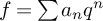 $f = \sum a_nq^n$
and
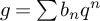 $g = \sum b_nq^n$
be primitive holomorphic modular cuspforms for
 $\Gamma _0(N),$
of weights k and l, with nebentypus characters
 $\chi $
and
 $\psi ,$
respectively. Let
 ${\mathbb Q}(f,g)$
be the number field obtained by adjoining the Fourier coefficients
 $\{a_n\}$
and
 $\{b_n\}$
to
 ${\mathbb Q}.$
Assume that
 $k> l.$
A well-known theorem of Shimura [Reference Shimura34] says that for
 $D_N(s, f,g),$
the degree-
 $4$
Rankin–Selberg L-function attached to the pair
 $(f,g)$
, and for any integer m with
 $l \leq m < k,$
we have
 $D_N(m,f,g) \approx (2\pi i)^{l+1-2m} \, {\mathfrak g}(\psi ) \, u^+(f)u^-(f),$
where
 $\approx $
means equality up to an element of
 ${\mathbb Q}(f,g)$
,
 $u^\pm (f)$
are the two periods attached to f by Shimura, and
 ${\mathfrak g}(\psi )$
is the Gauss sum of
 $\psi .$
The result may be refined and stated as a reciprocity law. The integers
 $l \leq m < k$
are all the critical points for
 $D_N(s, f,g).$
There are no critical points if
 $l = k.$
Suppose
 $k \geq l+2$
, and we look at two successive critical values; then the only change in the right-hand side is
 $(2\pi i)^{-2}$
, which is accounted for by the
 $\Gamma $
-factors at infinity. Suppose
 $L(s, f \times g)$
denotes the completed degree-
 $4 L$
-function attached to
 $(f,g)$
. Then we deduce
 $ L(l, f \times g) \ \approx \ L(l+1, f \times g) \ \approx \ \cdots \ \approx \ L(k-1, f \times g). $
The above result is a statement for L-functions for
 $\mathrm {GL}_2 \times \mathrm {GL}_2$
over
 ${\mathbb Q}.$
Shimura also generalized this to Hilbert modular forms [Reference Shimura35] (i.e., for
 $\mathrm {GL}_2 \times \mathrm {GL}_2$
over a totally real field
 $F).$
Since
 $(\mathrm {GL}_2 \times \mathrm {GL}_2)/\Delta \mathrm {GL}_1 \simeq \mathrm {GSO}(4),$
one may construe Shimura’s result as a theorem for the degree-
 $4 L$
-functions for certain orthogonal groups in four variables. The main theorem of this paper (see Theorem 1 below) generalises Shimura’s result as above to L-functions for
 $\mathrm {GL}_1 \times \mathrm {O}(2n)$
over a totally real number field F for an even positive integer n. The principal innovation of this article is that it offers new results on the arithmetic properties of L-functions for classical groups, outside the framework of general linear groups, via the Langlands–Shahidi theory of automorphic L-functions. We generalise the work of Harder and the second author [Reference Harder and Raghuram16] to study Eisenstein cohomology for
 $\mathrm {O}(2n+2)$
, while using Arthur’s classification [Reference Arthur1] as refined by Atobe–Gan [Reference Atobe and Gan2] for even orthogonal groups, to give a cohomological interpretation to certain aspects of the Langlands–Shahidi machinery [Reference Shahidi33].
We consider the split orthogonal group
 $\mathrm {O}(2n)$
defined by the matrix
 $J_{2n}$
(see (4)) which has
 $1$
’s along the anti-diagonal and
 $0$
’s elsewhere. For now, we let
 $G = \mathrm {Res_{F/{\mathbb Q}}}(\mathrm { O}(2n)/F)$
be the group over
 ${\mathbb Q}$
given by Weil restriction of scalars from
 $F/{\mathbb Q}$
. (Later, G will be a bigger orthogonal group and
 $\mathrm {Res_{F/{\mathbb Q}}}(\mathrm {O}(2n)/F)$
will be an almost simple factor of the Levi quotient of a particular parabolic subgroup of G.) Let
 ${\mathbb A}$
denote the adèle ring of
 ${\mathbb Q}$
, and
 ${\mathbb A}_f$
be the finite adèles. For an open-compact subgroup
 $K_f$
of
 $G({\mathbb A}_f)$
we denote the adèlic locally symmetric space with level structure
 $K_f$
by
 ${\mathcal S}^{G}_{K_f}.$
These notions are defined in Section 1. Let T be the restriction of scalars of the diagonal torus in
 $\mathrm {O}(2n)$
. We take a large enough finite Galois extension E of
 ${\mathbb Q}$
containing a copy of F. Let
 $\lambda \in X^*(T \times E)$
be a dominant integral weight, and
 ${\mathcal M}_{\lambda ,E}$
be the algebraic finite-dimensional absolutely irreducible representation of
 $G \times E$
with highest weight
 $\lambda $
. Let
 $\widetilde {{\mathcal M}}_{\lambda ,E}$
be the associated sheaf of E-vector spaces on
 ${\mathcal S}^{G}_{K_f}.$
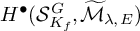
A fundamental object of study is the cohomology
 $H^{\bullet } ({\mathcal S}^{G}_{K_f}, \widetilde {{\mathcal M}}_{\lambda ,E})$
of the space
 ${\mathcal S}^{G}_{K_f}$
with coefficients in the sheaf
 $\widetilde {\mathcal {M}}_{\lambda ,E}.$
A basic tool to study these cohomology groups is the long exact sequence attached to the Borel–Serre compactification
 $\overline {\mathcal S}^{G}_{K_f} = {\mathcal S}^{G}_{K_f} \cup \partial {\mathcal S}^{G}_{K_f}:$
 $$ \begin{align*}\cdots \xrightarrow{} {H^{\bullet}_{c}({\mathcal S}^{G}_{K_f}, \widetilde{{\mathcal M}}_{\lambda,E} )} \xrightarrow{\mathfrak{i}^{\bullet}} H^{\bullet} ({\mathcal S}^{G}_{K_f}, \widetilde{{\mathcal M}}_{\lambda,E} ) \xrightarrow{\mathfrak{r}^{\bullet}} H^{\bullet} (\partial {\mathcal S}^{G}_{K_f}, \widetilde{{\mathcal M}}_{\lambda,E} ) \xrightarrow{\partial^{\bullet}} H^{\bullet}_c({\mathcal S}^{G}_{K_f}, \widetilde{{\mathcal M}}_{\lambda,E} ) \xrightarrow{} \cdots\end{align*} $$
This is a sequence of
 $\mathcal H^{G}_{K_{f}}$
-modules, where
 $\mathcal H^{G}_{K_{f}}$
is a suitable Hecke-algebra over
 ${\mathbb Q}$
defined as the restricted tensor-product of local Hecke algebras. For a finite set S of places including the archimedean and ramified places, we let
 $\mathcal H^{G,S}$
denote the central subalgebra of
 $\mathcal H^{G}_{K_{f}}$
by taking the restricted tensor product over all places not in S. We often consider the above cohomology groups as modules over
 $\mathcal H^{G,S}$
.
Inner (or interior) cohomology
 $H^{\bullet }_{!}$
is defined as the image of
 $\mathfrak {i}^{\bullet }$
(i.e., the image of cohomology with compact supports inside total cohomology), and complementary to it is Eisenstein cohomology defined as the image of
 $\mathfrak {r}^{\bullet }$
(i.e., image of the total cohomology in the cohomology of the boundary). In Section 3.1, we define strongly-inner cohomology
 $H^{\bullet }_{!!}$
which is a subspace of
 $H^{\bullet }_{!}.$
The definition is motivated by [Reference Harder and Raghuram16], where strongly-inner cohomology is defined for
 $\mathrm {GL}_N/F$
having the virtue that under any embedding
 $\iota : E \to {\mathbb C}$
, rendering the context transcendental, strongly-inner cohomology base-changes to cuspidal cohomology. However, the general linear group dealt with in [Reference Harder and Raghuram16] is misleadingly simple. In the context of orthogonal groups, we appeal to Arthur’s classification of the discrete spectrum as expounded by Atobe–Gan [Reference Atobe and Gan2] and offer a definition of strongly-inner cohomology defined over E which captures an essential part of the cuspidal cohomology of G (see Defintion 25). If
 $\sigma _f$
is a
 $\mathcal H^{G}_{K_{f}}$
-module appearing in
 $H^{\bullet }_{!!}$
, then for any embedding
 $\iota : E \to {\mathbb C}$
, there is a cuspidal automorphic representation
 ${}^\iota \sigma $
of
 $\mathrm {O}(2n)$
over F such that (i)
 ${}^\iota \sigma $
is globally generic for a pre-specified Whittaker datum
 $\psi $
; (ii) the Arthur parameter
 $\Psi ({}^{\iota }\sigma )$
of
 ${}^\iota \sigma $
is a cuspidal representation of
 $\mathrm {GL}_{2n}/F$
; (iii) for each archimedean place v of F,
 ${}^{\iota }\sigma _v$
is the
 $\psi _{v}$
-generic discrete series representation of
 $\mathrm {O}(n,n)({\mathbb R})$
(recall that n is even) in the local L-packet defined by the weight
 ${}^{\iota }\mu ^{v}$
; (iv)
 $({}^\iota \sigma )_f^{{}^\circ C_f} = \sigma _f \otimes _{E, \iota } {\mathbb C}$
as
 $\mathcal H^{G}_{K_{f}}$
-modules over
 ${\mathbb C}.$
It is part of the defining property of strongly-inner cohomology that it provides a rational structure to an essential part of cuspidal cohomology of G. Strongly-inner cohomology is an ad hoc replacement of Clozel’s results [Reference Clozel11] on rational structure on cuspidal cohomology for
 $\mathrm {GL}_n.$
Let
 $\chi ^{\circ }$
be a finite order Hecke character of F taking values in
 $E,$
and d be an integer. Let
 $\chi $
stand for the algebraic Hecke character of F with values in E which for an embedding
 $\iota : E \to {\mathbb C}$
gives a continuous homomorphism
 ${}^\iota \chi : F^\times \backslash {\mathbb A}_F^\times \to {\mathbb C}^\times $
of the form
 ${}^\iota \chi = {}^\iota \chi ^\circ \otimes |\ |^{-d}.$
For a strongly-inner Hecke summand
 $\sigma _f$
, given the cuspidal automorphic representation
 ${}^\iota \sigma $
as above, we consider the degree-
 $2n$
completed L-function
 $L(s, {}^\iota \chi \times {}^\iota \sigma ).$
This L-function should be construed as the Langlands–Shahidi L-function (see case
 $(D_{n,i})$
of Appendix A in Shahidi’s book [Reference Shahidi33]) attached to any summand in the restriction of
 ${}^\iota \sigma $
to
 $\mathrm {SO}(2n)/F$
and the character
 ${}^\iota \chi .$
An integer m is said to be critical for
 $L(s, {}^\iota \chi \times {}^\iota \sigma )$
if the L-factors at infinity on either side of the functional equation are regular at
 $s = m.$
Our main result on rationality properties of critical values of
 $L(s, {}^\iota \chi \times {}^\iota \sigma )$
is the following:
Theorem 1. Let
 $\mu \in X^*(T \times E)$
be a dominant integral weight; suppose
 $\mu = (\mu ^\tau )_{\tau : F \to E}$
, with
 $\mu ^\tau = (\mu ^\tau _1,\dots , \mu ^\tau _n)$
,
 $\mu ^\tau _j \in {\mathbb Z},$
and
 $\mu ^\tau _1 \geq \cdots \geq \mu ^\tau _{n-1} \geq |\mu ^\tau _n|.$
Define
 $$ \begin{align*}\mu_{\mathrm{min}} \ := \ \min \{\ |\mu^\tau_n| \ \}_{\tau : F \to E}. \end{align*} $$
Assume that
 $\mu _{\mathrm {min}} \geq 1.$
Let
 $\sigma _f$
be a Hecke summand appearing in the strongly-inner cohomology of
 $\mathrm {O}(2n)/F$
with coefficients in
 $\widetilde {{\mathcal M}}_{\mu ,E}.$
For an embedding
 $\iota : E \to {\mathbb C}$
, let
 ${}~^{\iota }\sigma $
be the cuspidal automorphic representation of
 $\mathrm {O}(2n)/F.$
Let
 $\chi {}^\circ $
be a finite-order Hecke character of F that takes values in E and
 $d \in {\mathbb Z},$
giving a character
 ${}^\iota \chi = {}^\iota \chi ^\circ \otimes |\ |^{-d}$
as above. We have
-
(i) The critical set of
 $L(s, {}^\iota \chi \times {}^\iota \sigma )$
is given by the
$2 \mu _{\mathrm {min}}$
consecutive integers The critical set is independent of
$$ \begin{align*}\{d+1-\mu_{\mathrm{min}}, \ d+2-\mu_{\mathrm{min}}, \ \ldots \ , \ d+\mu_{\mathrm{min}}-1, \ d+\mu_{\mathrm{min}} \}. \end{align*} $$
$\iota .$


Since
 $L(s, {}^\iota \chi \times {}^\iota \sigma ) = L(s - d, {}^\iota \chi ^\circ \times {}^\iota \sigma )$
, for rationality of critical values, we consider the critical values of
 $L(s, {}^\iota \chi ^\circ \times {}^\iota \sigma )$
without any loss of generality.
-
(ii) The assumption
$\mu _{\mathrm {min}} \geq 1$
guarantees the existence of at least two successive critical points. Suppose m and
$m+1$
are critical and
$m \neq 0$
. Then we have The above conclusion is also valid for
$$ \begin{align*}\frac{L(m, {}^\iota\chi^\circ \times {}^\iota \sigma) }{L(m+1, {}^\iota\chi^\circ \times {}^\iota \sigma)} \ \in \ \iota(E). \end{align*} $$
$m=0$
provided we assume furthermore that
${}^\iota \sigma $
is tempered at all finite places.
-
(iii) For every
$\eta \in \mathrm {Gal}(\bar {{\mathbb Q}}/ {\mathbb Q})$
, we have the reciprocity law:
$$ \begin{align*}\eta \left( \frac{L(m, {}^\iota\chi^\circ \times {}^\iota \sigma)}{L(m+1, {}^\iota\chi^\circ \times {}^\iota \sigma)}\right) \ = \ \frac{L(m, {}^{\eta\circ\iota}\chi^\circ \times {}^{\eta\circ\iota} \sigma)}{L(m+1, {}^{\eta\circ\iota}\chi^\circ \times {}^{\eta\circ\iota}\sigma)}. \end{align*} $$


The calculation of the critical set in
 $(i)$
follows from knowing the Langlands parameter of discrete series representations, which, together with the archimedean case of the local Langlands correspondence, gives us the local L-factor at infinity. See Section 4.2.
For the rest of the theorem, we follow the general framework of [Reference Harder and Raghuram16]; however, we encounter serious difficulties in that we are working with an orthogonal group and not a general linear group. For
 $(ii)$
and
 $(iii)$
, as in [Reference Harder and Raghuram16], there is an underlying combinatorial lemma (Section 5) which says that we need to prove a rationality result for one specific ratio of critical values for a general family, and then the result automatically follows for all ratios of successive critical values. The critical set calculation gives that the combinatorial condition
 $$ \begin{align} 1 - \mu_{\mathrm{min}} \ \leq \ -(d+n) \ \leq \ \mu_{\mathrm{min}} - 1 \end{align} $$
is equivalent to the fact that
 $s = -n$
and
 $s = 1-n$
are critical for
 $L(s, {}^\iota \chi \times {}^\iota \sigma ).$
Under this condition, we prove
 $$ \begin{align} \frac{L(-n, {}^\iota\chi \times {}^\iota \sigma) }{L(1-n, {}^\iota\chi \times {}^\iota \sigma)} \ \in \ \iota(E) \end{align} $$
and also prove a reciprocity law as in
 $(iii)$
for this particular ratio; then both
 $(ii)$
and
 $(iii)$
of the theorem follow by letting d vary as long as the combinatorial condition (2) is satisfied. It turns out that the constraint imposed on d by the inequalities in (2) exactly captures every successive ratio of critical values for
 $L(s, {}^\iota \chi ^\circ \times {}^\iota \sigma ),$
no more and no less!
The technical heart of the proof of (3) concerns rank-one Eisenstein cohomology for
 $\mathrm {O}(2n+2)/F$
and Langlands’s constant term theorem viewed in terms of maps in cohomology. Changing notations, henceforth we let
 $G = \mathrm {Res}_{F/{\mathbb Q}}(\mathrm {O}(2n+2)/F),$
and
 $P = \mathrm {Res}_{F/{\mathbb Q}}(P_0),$
where
 $P_0$
is the maximal parabolic subgroup of
 $\mathrm {O}(2n+2)/F$
whose Levi quotient is
 $M_0 = \mathrm {GL}_1/F \times \mathrm {O}(2n)/F.$
The combinatorial lemma also gives that the algebraically and parabolically induced representation
 ${}^{\mathrm {a}}\mathrm {Ind}_{P({\mathbb A}_f)}^{G({\mathbb A}_f)}(\chi _f \times \sigma _f)$
appears in the cohomology of the boundary in a very special degree; this involves combinatorial subtleties on Kostant representatives in Weyl groups. We prove a ‘Manin–Drinfeld principle’ (Theorem 69), which says that this induced representation together with its partner across an intertwining operator splits off as an isotypic component; this theorem uses results of Arthur and Atobe–Gan on the classification of the discrete spectrum for orthogonal groups. We then prove our main theorem on rank-one Eisenstein cohomology (Theorem 80), which says that the image of Eisenstein cohomology in this isotypic component is analogous to a line in a two-dimensional plane. If one passes to a transcendental situation using an embedding
 $\iota : E \to {\mathbb C}$
, then via Langlands’s constant term theorem, the slope of this line is the required ratio of L-values.
There are certain archimedean problems that need to be solved. First, Harish-Chandra’s classification of discrete series representations works best for a connected semisimple Lie group. For us, the (almost-)simple factor of the Levi group
 $M_0({\mathbb R})$
is
 $\mathrm {O}(n,n)({\mathbb R})$
, the real split orthogonal group, whose group of connected components has order
 $4$
. The action of this group of connected components on relative Lie algebra cohomology of the discrete series representation of
 $\mathrm {O}(n,n)({\mathbb R})^\circ = \mathrm {SO}(n,n)({\mathbb R})^\circ $
necessitates some arduous book-keeping; this is reviewed in Section 2 and applied later in 6.6.6. Next, we need a delicate analysis of the rationality properties of archimedean representations and intertwining operators; see Section 6.6. As in other contexts involving Eisenstein cohomology ([Reference Harder and Raghuram16], [Reference Raghuram29]), the point of evaluation
 $s = -n$
being a critical point, and if we are on the right of the unitary axis (see Section 6.5), then from general results of Casselman–Shahidi [Reference Casselman and Shahidi9], it follows that the induced representations at hand are irreducible and the standard intertwining operator is well-defined and finite at this point. We show in Proposition 62 that the map induced in relative Lie algebra cohomology by the archimedean standard intertwining operator contributes, up to nonzero rational numbers, the ratio of local archimedean L-values in (3).
As mentioned earlier, what is new in this article is that it represents the first serious study of the arithmetic properties of L-functions for classical groups, outside the framework of general linear groups, via a cohomological interpretation of certain parts of the Langlands–Shahidi theory of L-functions [Reference Shahidi33]. We expect our methods to pave the way to study the arithmetic of other families of automorphic L-functions. For
 $n=2,$
our results specialize to results of Shimura; however, for all even
 $n \geq 4$
, the results are new. A technically subtle point, the full import of which we had not appreciated in our announcement [Reference Bhagwat and Raghuram5], is our use of
 $\mathrm {O}(2n)$
and not
 $\mathrm {SO}(2n)$
; Arthur’s classification [Reference Arthur1] of the discrete spectrum for
 $\mathrm {SO}(2n)$
is only up to conjugation by the ambient
 $\mathrm {O}(2n)$
; this was finessed by Atobe and Gan [Reference Atobe and Gan2], who gave a satisfactory classification for the discrete spectrum for
 $\mathrm {O}(2n).$
In Section 9.3, amplifying on a comment made in [Reference Bhagwat and Raghuram5], we explain the need to work intrinsically with
 $\mathrm {O}(2n)$
, and not transfer to
 $\mathrm {GL}(2n)$
, to prove our main theorem on the special values of L-functions. Finally, our theorem on the rationality of ratios of successive critical values is compatible with Deligne’s conjecture [Reference Deligne and Ogus12] on the critical values of motivic L-functions. The reader is referred to the article of Deligne and the second author [Reference Deligne and Raghuram13], which gives a motivic explanation for a growing body of results on ratios of successive critical values including the main result of this article.
1 Preliminaries on the cohomology of orthogonal groups
1.1 The base field and algebraic groups
Let F be a totally real number field of degree
 $\mathsf {r}_F = [F: {\mathbb Q}].$
Let
 $\Sigma _F := \mathrm {Hom}(F, {\mathbb R}) = \mathrm {Hom}(F,{\mathbb C})$
be the set of all embeddings of F into
 ${\mathbb R}$
or
 ${\mathbb C},$
and denote by
 $S_{\infty }$
the set of archimedean places of F. Of course,
 $S_\infty $
is in bijection with
 $\Sigma _F.$
The completion of F at any place v is denoted
 $F_v.$
For
 $v \in S_{\infty }$
, we identify
 $F_{v}$
with
 ${\mathbb R}$
. Let
 $n = 2r \geq 2$
be an even integer. Let
 $G_{0} = \mathrm {O}(2n+2) / F$
be the split orthogonal group defined by the equation
 ${}^\intercal g~ J_{2n+2}~ g = J_{2n+2} $
, where
 ${}^\intercal g$
is the transpose of g, and for any positive integer m, the matrix
 $J_{m}$
is given by
 $$ \begin{align} J_{m} = \left( \begin{array}{ccc} & & 1 \\ & \unicode{x22F0} \\ 1 & & \end{array} \right)_{m \times m}. \end{align} $$
When the size m is clear from context, we will denote
 $J_m$
simply by
 $J.$
The subgroup
 $B_{0}$
consisting of all upper triangular matrices in
 $G_{0}$
defines a Borel subgroup of
 $G_0$
. Let
 $T_{0} \subset B_{0}$
be a split torus of
 $G_0$
consisting of the diagonal matrices. Let
 $N_0$
be the unipotent radical of
 $T_0$
in
 $B_0$
. So we have
 $B_0 = T_0 N_0$
. Let
 $G = R_{F / {\mathbb Q}} (G_{0} / F)$
be the group obtained by the Weil restriction of scalars to
 ${\mathbb Q}$
. Similarly, for
 $B_0$
,
 $T_0,$
and
 $N_0$
, we denote the
 ${\mathbb Q}$
-groups obtained from by restriction of scalars by B,
 $T,$
and N, respectively.
1.2 The groups at infinity
The group of real points of G is given by
 $$ \begin{align*}G({\mathbb R}) = \prod \limits_{v \in S_{\infty}} G(F_v) = \prod \limits_{v \in S_{\infty}} \mathrm{O}(n+1,n+1)({\mathbb R}). \end{align*} $$
The map
 $g \mapsto {}^\intercal g^{-1}$
defines a Cartan involution on
 $G({\mathbb R})$
, and its fixed points define a maximal compact subgroup
 $K_{\infty }$
of
 $G({\mathbb R})$
:
 $$ \begin{align*}K_{\infty} \ \simeq \ \prod \limits_{v \in S_{\infty}} \mathrm{O}(n+1)({\mathbb R}) \times \mathrm{O}(n+1)({\mathbb R}). \end{align*} $$
To describe this isomorphism explicitly, consider the map
 $$ \begin{align*}h : \mathrm{O}(n+1)({\mathbb R}) \times \mathrm{O}(n+1)({\mathbb R}) \ \longrightarrow \ \mathrm{O}(n+1,n+1)({\mathbb R}), \end{align*} $$
which is defined by
 $$ \begin{align} (k, l) \mapsto h(k, l) = \dfrac{1}{2} \begin{pmatrix} k + J l J & k J - J l \\ J k - l J & J k J + l \end{pmatrix}, \end{align} $$
where
 $k,l \in \mathrm {O}(n+1)({\mathbb R}),$
that is, they satisfy
 ${}^\intercal k \cdot k = I_{n+1} = {}^\intercal l \cdot l,$
and J in the formula above is
 $J_{n+1}.$
We leave it to the reader to check that h is a homomorphism and that the image of h lies in
 $\mathrm {O}(n+1,n+1)({\mathbb R})$
; that is, the map h gives an embedding of
 $\mathrm {O}(n+1)({\mathbb R}) \times \mathrm {O}(n+1)({\mathbb R}) \hookrightarrow \mathrm {O}(n+1,n+1)({\mathbb R})$
. For
 $v \in S_{\infty }$
, let
 $K_{v}$
be the image of
 $\mathrm {O}(n+1)({\mathbb R}) \times \mathrm {O}(n+1)({\mathbb R})$
inside
 $G_{v}$
, and put
 $K_{\infty } = \prod \limits _{v \in S_{\infty }}K_{v}$
; its connected component of the identity is
 $K^{\circ }_{\infty }$
, which is isomorphic to
 $\prod \limits _{v \in S_{\infty }} \mathrm {SO}(n+1)({\mathbb R}) \times \mathrm {SO}(n+1)({\mathbb R})$
and the component groups
 $ \pi _{0}(G({\mathbb R})) = \pi _{0}(K_{\infty }) \ \simeq \ ({\mathbb Z}/ 2{\mathbb Z} \times {\mathbb Z}/ 2{\mathbb Z})^{\mathsf {r_F}}.$
For any
 $m \geq 1$
, let’s write
 $\delta _m = \mathrm {diag}(-1,1,\dots ,1),$
and put
 $\mathrm {SO}(m)({\mathbb R})^\dagger := \mathrm {SO}(m)({\mathbb R})\delta _m.$
Then
 $\mathrm {SO}(m)({\mathbb R})$
and
 $\mathrm {SO}(m)({\mathbb R})^\dagger $
are the connected components of
 $\mathrm {O}(m)({\mathbb R}).$
For
 $v \in S_\infty $
, define a subgroup
 $\overline {K}_{v}$
of
 $K_v$
by
 $$ \begin{align} \overline {K}_{v} \ := \ h(\mathrm{SO}(n+1)({\mathbb R}) \times \mathrm{SO}(n+1)({\mathbb R})) \cup h(\mathrm{SO}(n+1)({\mathbb R})^\dagger \times \mathrm{SO}(n+1)({\mathbb R})^\dagger) \end{align} $$
and let
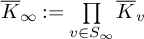 $\overline {K}_{\infty } : = \prod \limits _{v \in S_{\infty }} \overline {K}_{v} $
. The component group of
 $\overline {K}_{\infty }$
will be described later and will be used in the context of boundary cohomology.
1.3 Adèlic locally symmetric spaces
Let
 ${\mathbb A}$
be the ring of adèles of
 ${\mathbb Q}$
, and
 ${\mathbb A}_f$
denote the finite adèles. Let
 $K_{f} = \prod \limits _{v \notin S_{\infty }} K_v \subset G({\mathbb A}_{f})$
be an open compact subgroup. We will work with the adèlic symmetric space for G defined by
 $$ \begin{align*}{\mathcal S}^{G}: = G({\mathbb A}) / \overline{K}_{\infty} K_{f} = G({\mathbb R})/\overline{K}_{\infty} \times G({\mathbb A}_f)/K_{f}.\end{align*} $$
The discrete subgroup
 $G({\mathbb Q})$
of
 $G({\mathbb A})$
acts properly discontinuously on
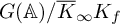 $G({\mathbb A}) / \overline {K}_{\infty } K_{f} $
. The adèlic locally symmetric space
 ${\mathcal S}^{G}_{K_{f}}$
, with level structure
 $K_{f} $
is the quotient space given by
 $$ \begin{align*}G({\mathbb A}) / \overline{K}_{\infty} K_{f} \twoheadrightarrow G({\mathbb Q}) \backslash G({\mathbb A}) /\overline{K}_{\infty} K_{f}. \end{align*} $$
Note the technical artifice of dividing by
 $\overline {K}_{\infty }$
; this will be useful later (see Section 6.6.6). In principle, we can divide by any subgroup in between
 $K_\infty ^\circ $
and
 $K_\infty .$
When we associate similar locally symmetric spaces for Levi subgroups of G, and compute the action of the group of components on the cohomology of a discrete series representation, in preparation to describe parts of the cohomology of the Borel–Serre boundary, then the virtue of dividing by
 $\overline {K}_\infty $
will become clear. The level structure
 $K_f$
will be assumed to be neat, which ensures that for any
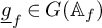 $\underline g_f \in G({\mathbb A}_f)$
, the discrete subgroup
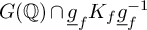 $G({\mathbb Q}) \cap \underline g_f K_f \underline g_f^{-1}$
of
 $G({\mathbb R})$
is torsion free. Given any open compact subgroup
 $K_f$
, we may pass to a subgroup of finite index which is neat. Later, we will also assume that
 $K_f$
is a principal congruence subgroup (see 7.2.2).
1.4 The character module and dominant integral weights
Let E be a ‘large enough’ finite Galois extension of
 ${\mathbb Q}$
such that
 $\mathrm {Hom}(F, {\mathbb R}) = \mathrm {Hom}(F, E)$
. The meaning of ‘large enough’ is usually clear from the context; we will want some Hecke summands in inner cohomology to split over E. Let
 $X^{\ast }(T \times E) = \mathrm {Hom}_{\mathrm {alg}} (T \times E, \mathbb G_m)$
be the group of characters of
 $T \times E.$
We have
 $$ \begin{align*}X^*(T \times E) = \bigoplus_{\tau : F \to E} X^{\ast}(T_{0} \times_{F, \tau} E). \end{align*} $$
A character
 $\lambda \in X^*(T \times E),$
also called an integral weight for T, will be written in the above decomposition as
 $\lambda = (\lambda ^\tau )_{\tau : F \to E},$
with
 $\lambda ^\tau \in X^*(T_0 \times _{F,\tau } E) = \mathrm {Hom}_{\mathrm {alg}} (T_0 \times _{F,\tau } E, \mathbb G_m);$
furthermore, we write
 $\lambda ^{\tau } = (\lambda _0^{\tau }, \lambda _1^{\tau }, \ldots , \lambda _n^{\tau }),$
with integrality of
 $\lambda $
meaning that
 $\lambda ^\tau _j \in {\mathbb Z}$
, and describe its values on elements of the diagonal torus by
 $$ \begin{align*}\lambda^{\tau}(\text{diag} [ t_0, \ldots, t_n, t_n^{-1}, \ldots, t_{0}^{-1} ]) \ = \ \prod \limits_{i=0}^{n} t_i^{\lambda_i^{\tau}}. \end{align*} $$
The Galois group
 $\mathrm {Gal} (E / {\mathbb Q})$
acts on
 $X^{\ast }(T \times E)$
by
 $ ({}^{\eta } \lambda )^{\tau } : = \lambda ^{\eta ^{-1} \circ \tau },$
for all
 $\lambda \in X^{\ast }(T \times E), \tau : F \to E$
, and
 $\eta \in \mathrm {Gal} (E / {\mathbb Q}).$
An integral weight
 $\lambda = (\lambda ^{\tau })_{\tau : F \rightarrow E} \in X^{\ast }(T \times E)$
is said to be a dominant with respect to Borel subgroup B if for all
 $\tau : F \to E$
, we have
 $$ \begin{align*}\lambda_0^{\tau} \geq \lambda_1^{\tau} \geq \ldots \geq \lambda_{n-1}^{\tau} \geq |\lambda_{n}^{\tau}|. \end{align*} $$
We denote the set of dominant integral weights for T by
 $X^{\ast }_{+}(T \times E)$
.
1.5 The sheaf
$\widetilde {\mathcal M}_{\lambda , E}$
and its cohomology

1.5.1
Let
 $G^{\circ } = \mathrm {Res}_{F/{\mathbb Q}}(\mathrm {SO}(2n+2)/F)$
denote the connected component of the identity of
 $G.$
Given
 $\lambda = (\lambda ^{\tau })_{\tau : F \rightarrow E} \in X^{\ast }_+(T \times E)$
as above, let
 $(\rho _{\lambda }, \mathcal N_{\lambda , E})$
be the absolutely irreducible finite-dimensional representation of the group
 $G^{\circ } \times E$
with highest weight
 $\lambda $
. Consider the induced representation
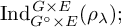 $\mathrm {Ind}^{\, G \times E }_{G^{\circ } \times E} (\rho _{\lambda });$
we denote its representation space as
 $\mathcal M_{\lambda , E}$
. We may parse
 ${\mathcal M}_{\lambda , E}$
over the embeddings
 $\tau : F \to E$
as follows: let
 $\mathcal N_{\lambda ^{\tau }, E}$
be the absolutely irreducible finite-dimensional representation of
 $\mathrm {SO}(2n+2) \!\times _{F, \tau }\!E$
with highest weight
 $\lambda ^{\tau }$
; induce
 $\mathcal N_{\lambda ^{\tau }, E}$
to a representation
 ${\mathcal M}_{\lambda ^{\tau }, E}$
of
 $\mathrm {O}(2n+2) \!\times _{F, \tau }\!E$
. Then
 $$ \begin{align*} {\mathcal M}_{\lambda, E} = \bigotimes_{\tau: F \rightarrow E} \mathcal M_{\lambda^{\tau}, E}. \end{align*} $$
The tensor product is of E-vector spaces.
1.5.2
Consider the quotient map
 $ \pi : G(\mathbb A) / \overline {K}_{\infty } K_{f} \rightarrow G({\mathbb Q}) \backslash G(\mathbb A) / \overline {K}_{\infty } K_{f} $
. The representation
 ${\mathcal M}_{\lambda ,E}$
gives a sheaf
 $\widetilde {\mathcal M}_{\lambda ,E}$
of E-vector spaces on the space
 ${\mathcal {S}}^G_{K_{f}}$
defined as follows: the sections over any open subset V of
 ${\mathcal {S}}^G_{K_{f}}$
are given by
 $$ \begin{align*} \widetilde{\mathcal M}_{\lambda,E}(V) \ := \ \{s: \pi^{-1}(V) \rightarrow \mathcal M_{\lambda,E} \ | \ s\text{ is smooth, and} \\ s(\gamma \underline x) = \rho_{\lambda}(\gamma) s(\underline x), \ \forall~\gamma \in G({\mathbb Q}), \ \underline x \in \pi^{-1}(V) \}, \end{align*} $$
where, smooth means locally constant at non-archimedean places, and infinitely differentiable at the archimedean places.
1.5.3
Analogous to [Reference Harder and Raghuram16, Lem. 2.3], we need to ask the following question: Under what conditions is the sheaf
 $\widetilde {\mathcal {M}}_{\lambda , E}$
nonzero? In our context, this has an easy answer: Suppose
 $Z_0$
is the center of
 $G_0$
and
 $Z = \mathrm {Res}_{F/{\mathbb Q}}(Z_0)$
, then
 $Z({\mathbb Q}) = Z_0(F) = \{\pm I\}$
. It is easy to see that
 $Z({\mathbb Q}) \cap \overline {K}_\infty $
is trivial. Hence, we deduce that the sheaf
 $\widetilde {\mathcal {M}}_{\lambda , E}$
is nonzero. Of course, since the center is finite, and since we may replace
 $K_f$
by a finite-index subgroup, we are guaranteed that
 $Z({\mathbb Q}) \cap \overline {K}_\infty K_f$
is trivial.
1.6 The cohomology of
$\widetilde {\mathcal M}_{\lambda , E}$

1.6.1
A fundamental object of interest is the cohomology
 $H^\bullet (\mathcal {S}^G_{K_f}, \widetilde {\mathcal {M}}_{\lambda , E})$
of the space
 $\mathcal {S}^G_{K_f}$
with coefficients in the sheaf
 $\widetilde {\mathcal {M}}_{\lambda , E}.$
At this point, the reader is referred to [Reference Harder and Raghuram16, Sect. 2.3] for generalities on these cohomology groups. We will be brief here in an effort to make this article reasonably self-contained. Let
 $\mathcal {H}^G_{K_f} = C^\infty _c(G({\mathbb A}_f)/ \! \!/K_f)$
be the set of all locally constant and compactly supported bi-
 $K_f$
-invariant
 ${\mathbb Q}$
-valued functions on
 $G({\mathbb A}_f).$
Take the Haar measure on
 $G({\mathbb A}_f)$
to be the product of local Haar measures, and for every prime p, the local measure is normalized so that
 $\mathrm {vol}(G({\mathbb Z}_p)) = 1.$
Then
 $\mathcal {H}^G_{K_f}$
is a
 ${\mathbb Q}$
-algebra under convolution. We have an action of
 $\pi _0(G({\mathbb R})) \times \mathcal {H}^G_{K_f}$
on
 $H^\bullet (\mathcal {S}^G_{K_f}, \widetilde {\mathcal {M}}_{\lambda , E}).$
Functorial properties of the sheaves
 $\widetilde {\mathcal {M}}_{\lambda , E}$
upon changing the field E are relevant for Galois actions on the cohomology groups
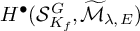 $H^\bullet (\mathcal {S}^G_{K_f}, \widetilde {\mathcal {M}}_{\lambda , E})$
, and also for the relation of these cohomology groups with automorphic forms using an embedding
 $\iota : E \to {\mathbb C}$
that gives a map
 $\iota ^\bullet : H^\bullet (\mathcal {S}^G_{K_f}, \widetilde {\mathcal {M}}_{\lambda , E}) \to H^\bullet (\mathcal {S}^G_{K_f}, \widetilde {\mathcal {M}}_{{}^\iota \!\lambda , {\mathbb C}}).$
The embedding
 $\iota $
gives a bijection
 $\iota _* : \mathrm {Hom}(F,E) \to \mathrm {Hom}(F,{\mathbb C})$
via composition. The weight
 ${}^\iota \!\lambda $
may be described by
 ${}^\iota \!\lambda = (({}^\iota \!\lambda )^\tau )_{\tau : F \to {\mathbb C}}$
where
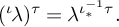 $({}^\iota \!\lambda )^\tau = \lambda ^{\iota _*^{-1}\tau }.$
1.6.2 A long exact sequence.
Let
 $ \bar {\mathcal {S}}^G_{K_f}$
be the Borel–Serre compactification of
 $\mathcal {S}^G_{K_f}$
; that is,
 $ \bar {\mathcal {S}}^G_{K_f} = \mathcal {S}^G_{K_f} \cup \partial \mathcal {S}^G_{K_f}$
, where the boundary is stratified as
 $\partial \mathcal {S}^G_{K_f} = \cup _P \partial _P\mathcal {S}^G_{K_f},$
with P running through the
 $G({\mathbb Q})$
-conjugacy classes of proper parabolic subgroups defined over
 ${\mathbb Q}$
. (See Borel–Serre [Reference Borel and J-P7].) The sheaf
 $\widetilde {\mathcal {M}}_{\lambda , E}$
on
 $\mathcal {S}^G_{K_f}$
naturally extends to a sheaf on
 $ \bar {\mathcal {S}}^G_{K_f}$
that we also denote by
 $\widetilde {\mathcal {M}}_{\lambda , E}$
. The inclusion
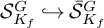 $\mathcal {S}^G_{K_f} \hookrightarrow \bar {\mathcal {S}}^G_{K_f}$
is a homotopy equivalence, and hence, the restriction from
 $ \bar {\mathcal {S}}^G_{K_f}$
to
 $\mathcal {S}^G_{K_f}$
induces an isomorphism in cohomology
 The cohomology of the boundary
 $H^\bullet (\partial \mathcal {S}^G_{K_f}, \widetilde {\mathcal {M}}_{\lambda , E})$
and the cohomology with compact supports
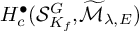 $H^\bullet _c(\mathcal {S}^G_{K_f}, \widetilde {\mathcal {M}}_{\lambda , E})$
are naturally modules for
 $ \pi _0(G({\mathbb R})) \times \mathcal {H}^G_{K_f}.$
We have the following long exact sequence of
 $\pi _0(G({\mathbb R})) \times \mathcal {H}^G_{K_f}$
-modules:
 $$ \begin{align*}\cdots \longrightarrow H^\bullet_c(\mathcal{S}^G_{K_f}, \widetilde{\mathcal{M}}_{\lambda, E})\stackrel{\mathfrak{i}^\bullet}{\longrightarrow} H^\bullet( \bar{\mathcal{S}}^G_{K_f}, \widetilde{\mathcal{M}}_{\lambda,E})\stackrel{\mathfrak{r}^\bullet}{\longrightarrow } &H^\bullet(\partial \mathcal{S}^G_{K_f}, \widetilde{\mathcal{M}}_{\lambda,E}) \\&\quad\ \ \ \xrightarrow{\partial^{\bullet}}H^{\bullet}_c(\mathcal{S}^G_{K_f}, \widetilde{\mathcal{M}}_{\lambda,E}) \longrightarrow \cdots . \end{align*} $$
1.6.3 Inner and Eisenstein cohomology.
The image of cohomology with compact supports inside the full cohomology is called inner or interior cohomology and is denoted
 $H^{\bullet }_{\, !}(\mathcal {S}^G_{K_f}, \widetilde {\mathcal {M}}_{\lambda , E}) := \mathrm {Image}(\mathfrak {i}^\bullet ).$
Complementary to inner cohomology is Eisenstein cohomology, defined as
 $H^\bullet _{\mathrm {Eis}}(\partial {\mathcal {S}^G_{K_f}}, \widetilde {\mathcal {M}}_{\lambda ,E}) := \mathrm {Image}(\mathfrak {r}^\bullet ).$
Let us note that neither inner cohomology nor Eisenstein cohomology is not an honest-to-goodness cohomology theory; however, the terminology is very convenient and helps with our geometric intuition with the nature of the cohomology classes therein. Functorial properties on changing the base field E apply verbatim to the cohomology groups
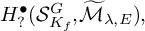 $H^\bullet _?(\mathcal {S}^G_{K_f}, \widetilde {\mathcal {M}}_{\lambda ,E}),$
where
 $? \in \{empty, c,!,\partial \};$
by
 $H^\bullet _\partial (\mathcal {S}^G_{K_f}, \widetilde {\mathcal {M}}_{\lambda ,E})$
we mean
 $H^\bullet (\partial {\mathcal {S}^G_{K_f}}, \widetilde {\mathcal {M}}_{\lambda ,E}).$
1.6.4 Cohomology of a boundary stratum
$\partial _P\mathcal {S}^G_{K_f}$
.

There is a spectral sequence whose
 $E_1^{pq}$
-term is built from the cohomology of various boundary strata
 $\partial _P\mathcal {S}^G_{K_f}$
that converges to the cohomology of
 $\partial {\mathcal {S}^G_{K_f}}$
(see [Reference Harder and Raghuram16, Sect. 4.1]). For the moment, P will denote any (representative of a
 $G({\mathbb Q})$
-conjugacy class of a) proper maximal parabolic subgroup of G, but from Section 1.7, it will denote a particular parabolic subgroup. The cohomology of any individual boundary strata
 $\partial _P\mathcal {S}^G_{K_f}$
is described in terms of representations induced from the cohomology of the Levi quotient of that boundary strata; we will briefly recall the essentials here while referring the reader to [Reference Harder and Raghuram16, Sect. 4.2] for more details. It is convenient to pass to the limit over all open-compact subgroups
 $K_f$
and define
 $$ \begin{align*}H^\bullet(\partial_P\mathcal{S}^G, \widetilde{\mathcal{M}}_{\lambda,E}) \ := \ \varinjlim_{K_f} \, H^\bullet(\partial_P\mathcal{S}^G_{K_f}, \widetilde{\mathcal{M}}_{\lambda,E}),\\[-20pt] \end{align*} $$
on which there is an action of
 $G({\mathbb A}_f)$
; for a given
 $K_f$
, we may retrieve
 $H^\bullet (\partial _P\mathcal {S}^G_{K_f}, \widetilde {\mathcal {M}}_{\lambda ,E})$
by taking the
 $K_f$
invariants:
 $H^\bullet (\partial _P\mathcal {S}^G, \widetilde {\mathcal {M}}_{\lambda ,E})^{K_f}.$
Let
 $\kappa _P : P \to P/U_P = M_P$
be the canonical map from P onto its Levi quotient
 $M_P$
by going modulo its unipotent radical
 $U_P.$
Define
 $K^{M_P}_\infty = \kappa _P(P({\mathbb R}) \cap \overline {K}_\infty );$
later, we will carefully analyse the inner structure of
 $K^{M_P}_\infty ,$
for a particular maximal parabolic subgroup. For any level structure
 $C_f \subset M_P({\mathbb A}_f)$
, define a locally symmetric space
 $$ \begin{align} \underline{\mathcal{S}}^{M_P}_{C_f} \ = \ M_P({\mathbb Q}) \backslash M_P({\mathbb A}) / K^{M_P}_\infty C_f. \end{align} $$
Again, it is convenient to pass to the limit over all open-compact subgroups
 $C_f;$
define
 $$ \begin{align*}H^\bullet(\underline{\mathcal{S}}^{M_P}, \widetilde{\mathcal{M}}) \ := \ \varinjlim_{C_f} \, H^\bullet(\underline{\mathcal{S}}^{M_P}_{C_f}, \widetilde{\mathcal{M}}). \end{align*} $$
We recall Proposition 4.2 of loc.cit.:
Proposition 8. The cohomology of the boundary stratum for P is given by
 $$ \begin{align*}H^\bullet(\partial_P\mathcal{S}^G, \widetilde{\mathcal{M}}_{\lambda,E}) \ = \ {}^{\mathrm{a}}\mathrm{Ind}_{\pi_0(P({\mathbb R})) \times P({\mathbb A}_f)}^{\pi_0(G({\mathbb R})) \times G({\mathbb A}_f)} \left( H^\bullet (\underline{\mathcal{S}}^{M_P}, \widetilde{H^\bullet(\mathfrak{u}_P, {\mathcal M}_{\lambda,E})} ) \right), \end{align*} $$
where the notations are as follows: The Lie algebra of
 $U_P$
is
 $\mathfrak {u}_P$
;
 $H^\bullet (\mathfrak {u}_P, {\mathcal M}_{\lambda ,E})$
is the Lie algebra cohomology of
 ${\mathcal M}_{\lambda ,E}$
that is naturally an
 $M_P$
-module giving us a sheaf on
 $\underline {\mathcal {S}}^{M_P}_{C_f};$
the cohomology group on the right-hand side is a module for
 $\pi _0(M_P({\mathbb R})) \times M_P({\mathbb A}_f);$
note that
 $\pi _0(M_P({\mathbb R})) = \pi _0(P({\mathbb R}))$
;
 ${}^{\mathrm {a}}\mathrm {Ind}$
stands for algebraic, or un-normalized, induction which is the usual notion for
 $P({\mathbb A}_f)$
to
 $G({\mathbb A}_f)$
, whereas induction from
 $\pi _0(P({\mathbb R}))$
to
 $\pi _0(G({\mathbb R}))$
means that we take invariants under the kernel of the canonical map
 $\pi _0(P({\mathbb R})) \to \pi _0(G({\mathbb R})).$
A celebrated theorem of Kostant [Reference Kostant23] asserts that as an
 $M_P \times E$
-module, one has a multiplicity-free decomposition
 $$ \begin{align} H^q(\mathfrak{u}_P, {\mathcal M}_{\lambda, E}) \ \simeq \ \bigoplus_{\substack{w \in W^P \\ l(w) = q}} {\mathcal M}_{w \cdot \lambda, E}, \end{align} $$
where
 $W^P$
is a special subset of the Weyl group of G consisting of all Kostant representatives (see Section 5.2 below), and for any element w in the Weyl group,
 $l(w)$
will denote its length defined in terms of simple reflections; the twisted action of w on a weight
 $\lambda $
is denoted
 $w \cdot \lambda ;$
see Section 5.1. When P is of the form
 $\mathrm {Res}_{F/{\mathbb Q}}(P_0)$
for a parabolic subgroup
 $P_0$
of
 $G_0$
, the elements of
 $W^P$
and the above decomposition of unipotent cohomology can be parsed over
 $\tau : F \to E$
as described in [Reference Harder and Raghuram16, Sect. 4.2.2]. Now, Proposition 8 together with (9) gives the following.
Proposition 10. The cohomology of
 $\partial _P\mathcal {S}^G$
is given by
 $$ \begin{align*}H^q(\partial_P\mathcal{S}^G, \widetilde{\mathcal{M}}_{\lambda, E}) \ = \ \bigoplus_{w \in W^P} {}^{\mathrm{a}}\mathrm{Ind}_{\pi_0(P({\mathbb R})) \times P({\mathbb A}_f)}^{\pi_0(G({\mathbb R})) \times G({\mathbb A}_f)} \left(H^{q - l(w)}(\underline{\mathcal{S}}^{M_P}, \widetilde{\mathcal{M}}_{w \cdot \lambda, E}) \right). \end{align*} $$
We will be especially interested in certain summands in the cohomology in some special degrees of the boundary stratum
 $\partial _P\mathcal {S}^G$
for one particular maximal parabolic subgroup P of G that we describe in the next subsection.
1.7 The root system for
$G_0$
and the maximal parabolic subgroup
$P_0$


The root system for
 $G_0$
with respect to the split torus
 $T_0$
is given by
 $\Delta _{G_0}: = \left\{ \pm e_i \pm e_j: 0 \leq i < j \leq n \right\},$
where
 $e_i$
is defined by
 $e_i (\text {diag} [ t_0, \ldots , t_n, t_n^{-1}, \ldots , t_{0}^{-1} ])= t_i$
for each
 $0 \leq i \leq n$
. The positive roots with respect to the Borel subgroup
 $B_0$
are
 $\Delta ^{+}_{G_0} = \left\{ e_i \pm e_j: 0 \leq i < j \leq n \right\}$
. Half the sum of positive roots for
 $G_0$
is
 $$ \begin{align*}{{\boldsymbol{\rho}}}_{G_{0}} = \sum \limits_{j=0}^{n} (n-j) e_j = ne_0 + (n-1) e_1 \ldots + 1e_{n-1} + 0e_n. \end{align*} $$
The simple roots are
 $$\begin{align*}\Pi_{G_0} \ := \ \{ \alpha_0 = e_0 - e_1, \ \ \alpha_1 = e_1 - e_2, \ \ \ldots \ \, \ \alpha_{n-1} = e_{n-1} - e_n, \ \ \alpha_n = e_{n-1} + e_n\}. \end{align*}$$
Henceforth, we let
 $P_0$
be the maximal parabolic subgroup of
 $G_0$
corresponding to deleting the first simple root
 $\alpha _0 = e_0 - e_1$
. The unipotent radical of
 $P_0$
is given by
 $$ \begin{align*}U_{P_0}= \left\{ u_{y_1, y_2, \ldots, y_{2n}} = \left( \begin{array}{ccccccc} 1 & y_1 & y_2 & \ldots & y_{2n} & 0 \\ & 1 & & & &-y_{2n} \\ & & 1 & & & -y_{2n-1} \\ & & & \ddots & & \vdots \ \\ & & & & \ddots & -y_{1} \\ & & & & & 1 \end{array}\right) \ \ | \ \ y_1,\dots,y_{2n} \in \mathbb G_{a} \right\}. \end{align*} $$
The Levi decomposition is
 $P_0 = M_{P_0} U_{P_0},$
where
 $$ \begin{align*}M_{P_0} = P_0 / U_{P_0} \cong A_0 \times {}^{\circ}M_{P_0}, \quad A_0 \cong \mathrm{GL}_1/F, \quad {}^{\circ}M_{P_0} \cong \mathrm{O}(2n)/ F. \end{align*} $$
In matrix form,
 $M_{P_0}$
is given by
 $$ \begin{align*}M_{P_0} = \left\{ \left( \begin{array}{ccc} x&& \\ &g& \\&&x^{-1} \end{array} \right) \ | \ x \in \mathrm{GL}(1), \ g \in \mathrm{O}(2n) \right\}. \end{align*} $$
We put
 $P = \mathrm {Res}_{F/{\mathbb Q}}(P_0).$
Then
 $M_P = \mathrm {Res}_{F/{\mathbb Q}}(M_{P_0})$
is its Levi quotient. The parabolic subgroup P of G being fixed, we often drop P from the notation. The diagonal torus
 $T_0$
of
 $G_0$
is contained in
 $M_0 := M_{P_0}$
, and we can write it as
 $T_0 = A_0 \times {}^\circ T_0$
, where
 ${}^\circ T_0$
is the diagonal torus in
 ${}^{\circ }M_0 := {}^\circ M_{P_0}.$
After restricting scalars from F to
 ${\mathbb Q}$
, we have
 $T = A \times {}^\circ T.$
The discussions about locally symmetric spaces, finite-dimensional algebraic representations, the corresponding sheaves and their cohomology for G are all applicable mutatis mutandis to
 ${}^\circ \! M := {}^\circ \! M_P = \mathrm {Res}_{F/{\mathbb Q}}({}^\circ \! M_{P_0}).$
1.8 Dimensions of certain adèlic locally symmetric spaces
Some piquant numerology involving various dimensions plays a role in our cohomology computations; for later use, we record some relevant dimensions. For notational simplicity, we will henceforth denote the groups
 $M_{P_0}/F$
and
 $^\circ M_{P_0}/F$
by
 $M_0$
and
 $^\circ M_{0}$
, respectively. The dimension of the locally symmetric space
 $\mathcal {S}^G_{K_f}$
for
 $G = \mathrm {Res}_{F/{\mathbb Q}}(\mathrm {O}(2n+2)/F)$
with level structure
 $K_f$
is
 $$ \begin{align*}\mathrm{dim}(\mathcal S^G_{K_f}) \ = \ \mathsf{r_F} \cdot (n+1)^2. \end{align*} $$
The dimension of its Borel–Serre boundary
 $\partial \mathcal S^G_{K_f}$
is
 $$ \begin{align*}\mathrm{dim}(\partial \mathcal S^G_{K_f}) \ = \ \mathsf{r_F} \cdot (n+1)^2 - 1. \end{align*} $$
Now consider
 $^{\circ }\!M = \mathrm {Res}_{F/{\mathbb Q}}(\mathrm {O}(2n)/F)$
; the connected component of the identity of the maximal compact subgroup
 $K_{{}^\circ \!M({\mathbb R})}$
of
 ${}^\circ \!M({\mathbb R})$
is
 $$ \begin{align*}K^{\circ}_{{}^\circ\!M({\mathbb R})} \ = \ \prod \limits_{\tau \in \Sigma_F} \mathrm{SO}(n) \times \mathrm{SO}(n), \end{align*} $$
and for any open-compact subgroup
 $K_{{}^{\circ }\!M_f}$
of
 ${}^{\circ }\!M({\mathbb A}_f)$
, we define
 $$ \begin{align} {\mathcal S}^{{}^\circ\!M}_{K_{{}^{\circ}\!M_f}} \ = \ {}^{\circ}\!M({\mathbb Q}) \backslash {}^{\circ}\!M({\mathbb A}) / K^{\circ}_{{}^\circ\!M({\mathbb R})} K_{{}^{\circ}\!M_f}. \end{align} $$
Whereas for
 $\mathcal {S}^G_{K_f}$
we divided by
 $\overline {K}_\infty $
which is in between the full maximal compact subgroup at infinity and its connected component, for
 $\mathrm {dim}(S^{{}^{\circ }\!M}_{K_{{}^{\circ }\!M_f}})$
, we divide by the connected component of the maximal compact subgroup at infinity. We have
 $$ \begin{align*}\mathrm{dim}({\mathcal S}^{{}^{\circ}\!M}_{K_{{}^{\circ}\!M_f}}) \ = \ \mathsf{r_F} \cdot n^2, \end{align*} $$
and its middle dimension (since n is even) is
 $$ \begin{align*}q_m \ := \ \dfrac{1}{2} ~\mathrm{dim} ~\mathcal S^{^{\circ}M}_{K_{{}^{\circ}M,f}} \ = \ \dfrac{ \mathsf{r_F} \cdot n^2}{2}. \end{align*} $$
This particular middle-dimension is interesting since it is only in this middle-degree that a discrete series representation of
 ${}^{\circ }M({\mathbb R})$
has nontrivial cohomology.
Write
 $M = A \times {}^{\circ }\!M$
, where
 $A = \mathrm {Res}_{F/{\mathbb Q}}(\mathrm {GL}_1)$
. Note that A contains a copy of
 $\mathbb G_m/{\mathbb Q}$
, which we denote by S. We have the group of real points:
 $$ \begin{align*}A({\mathbb R}) = \prod \limits_{\tau \in \Sigma_F} {\mathbb R}^{\times}, \quad {}^{\circ}\!M({\mathbb R}) = \prod \limits_{\tau \in \Sigma_F} \mathrm{O}(n,n)({\mathbb R}), \quad M({\mathbb R}) = A({\mathbb R}) \times {}^{\circ}\!M({\mathbb R}). \end{align*} $$
The group
 $S({\mathbb R}) = {\mathbb R}^\times $
sits diagonally in
 $A({\mathbb R})$
. Let
 $\kappa _P : P \to P/U_P = M$
be the canonical surjection. Let
 $C_f$
be the open compact subgroup of
 $M({\mathbb A}_f)$
defined by
 $$ \begin{align*}C_f = \kappa_P (K_f \cap P({\mathbb A}_f)). \end{align*} $$
We suppose that
 $K_f$
is such that we can write
 $C_f = B_f \times {}^{\circ }C_f,$
for an open compact subgroup
 $B_f$
of
 $A({\mathbb A}_f)$
and an open compact subgroup
 ${}^{\circ }C_f$
of
 ${}^{\circ }M({\mathbb A}_f)$
. Define the locally symmetric space for A as
 $$ \begin{align*}{\mathcal S}^{A}_{B_f} \ := \ A({\mathbb Q}) \backslash A({\mathbb A}) / S({\mathbb R})^{\circ}B_f \ = \ F^{\times} \backslash {\mathbb A}_{F}^{\times} / S({\mathbb R})^{\circ}B_f; \quad \dim({\mathcal S}^{A}_{B_f}) = \mathsf{r}_F-1, \end{align*} $$
and the locally symmetric space for M as
 $$ \begin{align} {\mathcal S}^{M}_{C_f} \ := \ {\mathcal S}^{A}_{B_f} \times {\mathcal S}^{{}^{\circ}\!M}_{{}^{\circ}C_f}. \end{align} $$
Hence, we see
 $$ \begin{align*}\dim({\mathcal S}^{M}_{C_f}) \ = \ \mathsf{r}_F -1 + \mathsf{r}_F \cdot n^2 \ = \ 2q_m + \mathsf{r}_F -1. \end{align*} $$
For later use, we denote
 $$ \begin{align} \begin{aligned} q_b \ & := \ q_m \ = \ \mathsf{r}_F \cdot n^2/2, \\ q_t \ & := \ q_m + \mathsf{r}_F -1 \ = \ \mathsf{r}_F \cdot n^2/2 + \mathsf{r}_F -1. \end{aligned} \end{align} $$
Note:
 $q_b + q_t = \dim ({\mathcal S}^{M}_{C_f}).$
Furthermore, let’s denote
 $$ \begin{align} \begin{aligned} \mathfrak{q}_b \ & := \ q_b + \tfrac{1}{2}\dim(U_P) \ = \ \mathsf{r}_F(n^2/2 + n), \\ \mathfrak{q}_t \ & := \ q_t + \tfrac{1}{2}\dim(U_P) \ = \ \mathsf{r}_F(n^2/2 + n +1)-1. \end{aligned} \end{align} $$
Note:
 $\mathfrak {q}_b + \mathfrak {q}_t = \mathrm {dim}(\partial \mathcal S^G_{K_f}).$
The subscripts
 $b, m$
and t are meant to suggest ‘bottom’, ‘middle’ and ‘top’.
1.9 Cohomology of spaces associated to the Levi subgroup
$M_P$

There is a delicate interplay between the various ‘locally symmetric spaces’ attached to the Levi quotient
 $M_P$
of our parabolic subgroup
 $P.$
As before, we abbreviate
 $M_P$
as
 $M.$
Here, we clarify the mutual relationship between these spaces and their cohomology. Fix a level structure
 $C_f \subset M({\mathbb A}_f)$
which we assume to be of the form
 $B_f \times {}^\circ \!C_f$
as in the previous subsection. Define
 $\tilde {{\mathcal S}}^{A}_{B_f} := A({\mathbb Q}) \backslash A({\mathbb A}) /B_f,$
and let
 $\theta _{A} : \tilde {{\mathcal S}}^{A}_{B_f} \to {\mathcal S}^{A}_{B_f}$
denote the canonical map which is a
 $S({\mathbb R})^\circ $
-fibration. Now define
 $$ \begin{align} \tilde{{\mathcal S}}^{M}_{C_f} \ := \ \tilde{{\mathcal S}}^{A}_{B_f} \times {\mathcal S}^{{}^{\circ}\!M}_{{}^{\circ}C_f}, \end{align} $$
which comes with the fibration
 $\theta _{M} : \tilde {{\mathcal S}}^{M}_{C_f} \to {\mathcal S}^{M}_{C_f},$
defined as
 $\theta _M = \theta _A \times 1_{{\mathcal S}^{{}^{\circ }\!M}_{{}^{\circ }C_f}}.$
We have the following spaces:
-
•
${\mathcal S}^{M}_{C_f}$
; defined in (12); it is the space that we can best refer to as the locally symmetric space attached to M. -
•
$\tilde {{\mathcal S}}^{M}_{C_f}$
, defined in (15); it comes with the fibration
$\theta _M : \tilde {{\mathcal S}}^{M}_{C_f} \to {\mathcal S}^{M}_{C_f}.$
-
•
$\underline {\mathcal {S}}^{M}_{C_f}$
, defined in (7); note that we have a finite-cover
$\tilde {{\mathcal S}}^{M}_{C_f} \to \underline {\mathcal {S}}^{M_P}_{C_f}$
whose fibre is the kernel of the map
$\pi _0(M({\mathbb R})) \to \pi _0(G({\mathbb R})).$






Let us clarify the relation between the cohomology groups attached to these spaces and a sheaf
 $\widetilde {\mathcal {M}}$
(which for us will be of the form
 $\widetilde {\mathcal {M}}_{\mu ,E}$
for a dominant integral weight
 $\mu $
for M) that is defined compatibly on all these three spaces. Denote
 $$ \begin{align} \overline{\pi_0}(M({\mathbb R})) \ := \ \mathrm{Kernel}\left(\pi_0(M({\mathbb R})) \to \pi_0(G({\mathbb R})) \right). \end{align} $$
In the description of the cohomology of a boundary stratum (see Proposition 10), one is naturally led to the cohomology of
 $\underline {\mathcal {S}}^{M}_{C_f}$
, which is related to the cohomology of
 $\tilde {{\mathcal S}}^{M}_{C_f}$
via
 $$ \begin{align} H^\bullet(\underline{\mathcal{S}}^{M}_{C_f}, \widetilde{\mathcal{M}}) \ = \ H^\bullet(\tilde{{\mathcal S}}^{M}_{C_f}, \widetilde{\mathcal{M}})^{\overline{\pi_0}(M({\mathbb R}))}. \end{align} $$
Next, the cohomology of the locally symmetric space
 ${\mathcal S}^{M}_{C_f}$
can be pulled back, via the map induced by
 $\theta _{M}$
, to the cohomology of
 $\tilde {{\mathcal S}}^{M}_{C_f}$
; that is, we have a map
 $$ \begin{align} \theta_M^* : H^\bullet({\mathcal S}^{M}_{C_f}, \widetilde{\mathcal{M}}) \ \to \ H^\bullet(\tilde{{\mathcal S}}^{M}_{C_f}, \widetilde{\mathcal{M}}). \end{align} $$
2 Discrete series representations and relative Lie algebra cohomology
For an archimedean place v of F, in this section, we review some basics for discrete series representations of
 ${}^{\circ }\!M_{P_0}(F_v)$
, which is the real split even orthogonal group
 $\mathrm {O}(n,n)({\mathbb R}).$
Some care needs to be exercised because of the disconnectedness of
 $\mathrm {O}(n,n)({\mathbb R}).$
We are especially interested in the action of its group of connected components on relative Lie algebra cohomology of discrete series representations.
2.1 Discrete series representations for a connected semisimple Lie group
We briefly review the general theory which is due to Harish-Chandra, and we refer the reader to Borel–Wallach [Reference Borel and Wallach8, II.5] for more details and references. Just for this subsection, we let G stand for a connected semisimple Lie group, and K a maximal compact subgroup of
 $G.$
Let
 $\mathfrak g$
and
 $\mathfrak k$
be the Lie algebras of G and K, respectively. Denote their complexfications as
 $\mathfrak {g}_{\mathbb C}$
and
 $\mathfrak {k}_{\mathbb C},$
respectively. Suppose that
 $\mathrm {rank}(G) = \mathrm {rank}(K)$
. Let
 $\mathfrak h$
be a Cartan subalgebra of both
 $\mathfrak g$
and
 $\mathfrak k$
, and
 $\mathfrak h_{{\mathbb C}}$
its complexification. Let
 $\Phi $
be the root system of
 $\mathfrak g_{{\mathbb C}}$
with respect to
 $\mathfrak h_{{\mathbb C}}$
and let
 $P(\Phi )$
be the weight lattice for
 $\Phi $
. A weight
 $\Lambda \in P(\Phi )$
is called regular if
 $\langle \Lambda , \alpha \rangle \neq 0 ~\text {for any} ~\alpha \in \Phi .$
A regular weight
 $\Lambda $
gives a positive system of roots and their half-sum:
 $$ \begin{align*}\Phi^+: = \{ \alpha \in \Phi: \langle \Lambda, \alpha \rangle> 0 \}, \quad {\boldsymbol{\rho}}: = \dfrac{1}{2} \sum \limits_{\alpha \in \Phi^+ } \alpha. \end{align*} $$
Denote the set of compact roots by
 $\Phi _K$
; a compact root is a root whose rootspace lies in
 $\mathfrak k_{{\mathbb C}}$
. The positive system
 $\Phi ^+$
gives a positive system for compact roots and their half-sum:
 $$ \begin{align*}\Phi^+_K: = \Phi_K \cap \Phi^+; \quad {\boldsymbol{\rho}}_K: = \frac{1}{2} \sum \limits_{\alpha \in \Phi^+_K } \alpha. \end{align*} $$
Let  be the Harish-Chandra isomorphism for the center
 $Z(\mathfrak U(\mathfrak g_{{\mathbb C}}))$
of the enveloping algebra
 $\mathfrak U(\mathfrak g_{{\mathbb C}})$
of
 $\mathfrak g_{{\mathbb C}};$
the Weyl group of G is denoted
 $W_G.$
For each regular weight
 $\Lambda \in P(\Phi )$
, we can associate a discrete series representation
 $\pi _{\Lambda }$
of G such that
-
(1) The infinitesimal character of
$\pi _{\Lambda }$
is
$\chi _{\Lambda }$
defined by
$\chi _{\Lambda }(z) = \Lambda (\gamma (z)), \forall z \in Z(\mathfrak U(\mathfrak g_{{\mathbb C}})).$
Thus,
$\pi _{\Lambda }$
and
$\pi _{\Lambda '}$
have same infinitesimal character if and only if there is
$w \in W_G$
such that
$w\lambda = \lambda '$
. -
(2) The lowest K-type of
${\pi _{\Lambda }}|_{K}$
has multiplicity one and its highest weight (called the Blattner parameter) is given by
$ \Lambda + {\boldsymbol {\rho }} - 2{\boldsymbol {\rho }}_K$
. -
(3) The representations
$\pi _{\Lambda }$
and
$\pi _{\Lambda '}$
are equivalent if there is
$w \in W_K,$
the Weyl group of K, such that
$w\Lambda = \Lambda '$
.








The following proposition describes the cohomology of a discrete series representation; see [Reference Borel and Wallach8, Prop. II.5.3].
Proposition 19. Let
 $(\pi _{\Lambda }, V)$
be a discrete series representation as above. Let
 $V_K$
be the
 $(\mathfrak g, K)$
-module of K-finite vectors in V. Let
 ${\mathcal M}$
be a finite-dimensional complex irreducible representation of G whose contragredient is denoted
 ${\mathcal M}^{\mathsf {v}}.$
-
(1) If the highest weight of
${\mathcal M} \neq \Lambda - {\boldsymbol {\rho }}$
, then
$\mathrm {Ext}^{\bullet }_{\mathfrak g, \mathfrak k} ({\mathcal M}, V_K) = 0.$
-
(2) If the highest weight of
${\mathcal M} = \Lambda - {\boldsymbol {\rho }}$
, then
$\mathrm {Ext}^{j}_{\mathfrak g, \mathfrak k} ({\mathcal M}, V_K) = 0,$
unless
$j = \tfrac {1}{2}\, \mathrm {dim}(G/K),$
and in this ‘middle-degree’ it is one-dimensional. -
(3) The relative Lie algebra cohomology
$H^{\bullet }(\mathfrak g, \mathfrak k;\, {\mathcal M}^{\mathsf {v}} \otimes H)$
is nonvanishing only when the highest weight of
${\mathcal M}$
is
$\Lambda - {\boldsymbol {\rho }}$
and the degree
$\bullet = \tfrac {1}{2}\, \mathrm {dim}(G/K)$
. In this case, it is one-dimensional and supported on the Blattner parameter.





2.2 Discrete series representations of orthogonal groups
Fix an archimedean place v of
 $F.$
Just for this Section 2.2, for brevity, we introduce these notations:
 ${}^\circ \!M := {}^{\circ }\!M_{P_0 v} = {}^{\circ }\!M_{P_0}(F_v) = \mathrm {O}(n,n)({\mathbb R}),$
the real split even orthogonal group;
 ${}^\circ \! M^\circ := {}^{\circ }\!M_{P_0 v}^\circ = \mathrm {SO}(n,n)({\mathbb R})^\circ ,$
the connected component of identity in
 ${}^\circ \!M$
;
 $K := K_{{}^{\circ }\!M_{P_0 v}} = \{g \in M \ | \ {}^{\intercal }g\,g = I_{2n} \}$
, the maximal compact subgroup of
 ${}^\circ \!M$
;
 $K^\circ := K_{{}^{\circ }\!M_{P_0 v}}^\circ ,$
the connected component of identity in
 $K,$
 ${}^{\circ }\mathfrak m$
the Lie algebra of
 ${}^\circ \!M$
or of
 ${}^\circ \!M^\circ $
, and
 $\mathfrak k$
the Lie algebra of K or of
 $K^\circ $
.
2.2.1 Representatives for the group of connected components.
The compact group K is isomorphic to
 $\mathrm {O}(n)({\mathbb R}) \times \mathrm {O}(n)({\mathbb R})$
, the isomorphism being the map h defined in (5), but after replacing
 $n+1$
by n. Inclusion induces an equality
 $\pi _0(K) = \pi _0({}^{\circ }\!M)$
of component groups; we give explicit representatives for elements of these component groups. Recall that
 $\delta _n = \mathrm {diag}(-1,1,\dots ,1)$
. Then
 $\pi _0(\mathrm {O}(n)({\mathbb R})) = \{I_n, \delta _n\}.$
Further, if
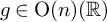 $g \in \mathrm {O}(n)({\mathbb R})$
, then clearly,
 $J_n\,g\,J_n \in \mathrm {O}(n)({\mathbb R}).$
Hence,
 $J_n \, \delta _n \, J_n$
also represents the nontrivial element of
 $\pi _0(\mathrm {O}(n)({\mathbb R})).$
We take as representatives for the connected components of
 $\mathrm {O}(n)({\mathbb R}) \times \mathrm {O}(n)({\mathbb R})$
the elements
 $$ \begin{align*}\{(I_n,I_n), \ (I_n, \delta_n), \ (J_n\delta_n J_n, I_n), \ (J_n\delta_n J_n, \delta_n)\}. \end{align*} $$
For any integer
 $m \geq 1$
, let
 $$ \begin{align} s_{2m}: = \begin{pmatrix} I_{m-1} & & \\ & -I_2 & \\ & & I_{m-1} \end{pmatrix}, \quad \text{and} \quad \kappa_{2m} : = \begin{pmatrix} I_{m-1} & & \\ & J_2 & \\ & & I_{m-1} \end{pmatrix}. \end{align} $$
One can check that
 $h(I_n,\delta _n) = \kappa _{2n}$
, and
 $h(J_n\delta _n J_n, \delta _n) = s_{2n}.$
Furthermore, one sees
 $$ \begin{align*}\kappa_{2n} \in \mathrm{O}(n,n)({\mathbb R}) \setminus \mathrm{SO}(n,n)({\mathbb R}), \quad s_{2n} \in \mathrm{SO}(n,n)({\mathbb R}) \setminus \mathrm{SO}(n,n)({\mathbb R})^{\circ}. \end{align*} $$
The component group
 $\pi _0(K)$
of K (as also
 $\pi _0({}^{\circ }M)$
of
 ${}^{\circ }M$
) is isomorphic to
 ${\mathbb Z}/2{\mathbb Z} \times {\mathbb Z}/2{\mathbb Z},$
and as representatives, we take
 $$ \begin{align*}\left\{I_{2n}, \ s_{2n}, \ \kappa_{2n}, \ s_{2n} \kappa_{2n} \right\}. \end{align*} $$
Note that
 $s_{2n} \kappa _{2n} = \kappa _{2n}s_{2n}.$
2.2.2 Compact Cartan subgroups and subalgebras.
At the level of Lie algebras, the same map h gives us
 $\mathfrak t_K$
, a compact Cartan subalgebra that is shared by both
 ${}^\circ \mathfrak {m}$
and
 $\mathfrak k_{{}^\circ \!M}$
, the Lie algebras of
 ${}^{\circ }\!M$
and
 $K,$
respectively. Let
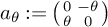 $a_{\theta }: = \left(\begin {smallmatrix} 0 & -\theta \\ \theta & 0 \end {smallmatrix}\right)$
for
 $\theta \in {\mathbb R}$
. Given
 $\theta _1, \ldots , \theta _n \in {\mathbb R}$
, let k and l be elements of
 ${\mathfrak s \mathfrak o}(n)$
, the Lie algebra of the compact
 $\mathrm {SO}(n)({\mathbb R})$
, defined by
 $$ \begin{align*}k = \begin{pmatrix} a_{\theta_1} && \\ &\ddots& \\ && a_{\theta_{r}} \end{pmatrix}, \quad l = \begin{pmatrix} a_{\theta_{r +1}} && \\ &\ddots& \\ && a_{\theta_{n}} \end{pmatrix}; \quad \text{recall that }n = 2r. \end{align*} $$
Then, we check that
 $$ \begin{align*}h(k,l) = \begin{pmatrix} a_{(\theta_1-\theta_n)/2} &&&&& a_{(\theta_1+\theta_n)/2}J_{2} \\ & \ddots && &\unicode{x22F0} & \\ && a_{(\theta_r-\theta_{r+1})/2} & \quad a_{(\theta_r+\theta_{r+1})/2}J_2 && \\ \\ && a_{-(\theta_r+\theta_{r+1})/2} J_2 & \quad a_{(\theta_{r+1}-\theta_{r})/2} && \\ & \unicode{x22F0} && & \ddots & \\ a_{-(\theta_1+\theta_n)/2}J_2 &&&&& a_{(\theta_n-\theta_1)/2} \end{pmatrix}. \end{align*} $$
Reparameterizing our variables,
 $$ \begin{align*}t_1 = \frac{\theta_1-\theta_n}{2}, \ \ \ t_2 = \frac{\theta_1+\theta_n}{2}, \ \ \dots, \ \ \ t_{n-1} = \frac{\theta_r-\theta_{r+1}}{2}, \ \ \ t_n = \frac{\theta_r+\theta_{r+1}}{2}, \end{align*} $$
we can describe the elements of the compact Cartan subalgebra as
 $$ \begin{align*}\mathfrak{t}_K \ = \ \left\{X_{t_1,\dots,t_n} := \begin{pmatrix} a_{t_1} &&&&& a_{t_2}J_{2} \\ & \ddots && &\unicode{x22F0} & \\ && a_{t_{n-1}} & \quad a_{t_n}J_2 && \\ && a_{-t_n} J_2 & \quad a_{-t_{n-1}} && \\ & \unicode{x22F0} && & \ddots & \\ a_{-t_2}J_2 &&&&& a_{-t_1} \end{pmatrix} \ | \ t_1, \dots, t_n \in {\mathbb R} \right\}. \end{align*} $$
Let
 $T_K$
be the analytic subgroup associated to
 $\mathfrak t_K$
inside
 $K^{\circ }$
. Consider the complexification
 $\mathfrak t_{K,{\mathbb C}}$
of
 $\mathfrak t_K$
; its elements are of the form
 $ X_{t_1, \ldots , t_n},$
where
 $t_j \in {\mathbb C}$
. It can be observed that all
 $ X_{t_1,\dots ,t_n} \in \mathfrak t_{K,{\mathbb C}}$
are simultaneously conjugate to elements of the complexified diagonal algebra
 $\mathfrak t_{{\mathbb C}}$
. The conjugating matrix can be taken in
 $\mathrm {O}(n,n)({\mathbb C})$
. Under this correspondence, the matrix
 $ X_{t_1,\dots ,t_n} \in \mathfrak t_{K,{\mathbb C}}$
is conjugate to the diagonal matrix
 $\mathrm {diag}[{\mathbf i}\theta _1, \ldots , {\mathbf i}\theta _n, -{\mathbf i}\theta _n, \ldots , -{\mathbf i}\theta _1] \in \mathfrak t_{{\mathbb C}}.$
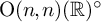
2.2.3 Roots and compact roots for
$\mathrm {O}(n,n)({\mathbb R})^\circ $
.
Recalling that
 ${\mathbf i}{\mathbb R}$
is the Lie algebra of the circle group
 $S^1$
, we define the linear functionals
 $e_i^K : \mathfrak t_K \to {\mathbf i} {\mathbb R},$
for
 $1 \leq i \leq n,$
as
 $$ \begin{align} \begin{aligned} e_1^K (X_{t_1,\dots,t_n}) & := \ {\mathbf i}(t_1 + t_2) = {\mathbf i} \theta_1, \quad e_2 ^K(X_{t_1,\dots,t_n}) : = \ {\mathbf i}(t_1 - t_2) = -{\mathbf i} \theta_n, \\ & \vdots \\ e_{n-1}^K (X_{t_1,\dots,t_n}) &: = \ {\mathbf i}(t_{n-1}+t_n) = {\mathbf i} \theta_r, \quad e_n^K (X_{t_1,\dots,t_n}) := {\mathbf i}(t_{n-1}-t_n) = -{\mathbf i} \theta_{r+1}. \end{aligned} \end{align} $$
It is clear then that
 $\{e_1^K,e_3^K,\dots ,e_{n-1}^K\}$
(resp.,
 $\{e_2^K,e_4^K,\dots ,e_n^K\}$
) are the linear functionals corresponding to the first (resp., second) summand of
 $\mathfrak {so}(n) \oplus \mathfrak {so}(n).$
The root system
 $\Phi $
of
 ${}^{\circ }\mathfrak {m}_{\mathbb C}$
with respect to
 $\mathfrak t_{K,{\mathbb C}}$
is given by
 $$ \begin{align*}\Phi = \{ \pm e_i^K \pm e_j^K \ | \ 1 \leq i < j \leq n \}. \end{align*} $$
The set of all compact roots
 $\Phi _K$
is
 $$ \begin{align*}\Phi_K = \{ \pm e_i^K \pm e_j^K \ | \ 1 \leq i < j \leq n, \ \ i \equiv j \ (\text{mod} \ 2)\}. \end{align*} $$
The weight lattice is given by
 $$ \begin{align*}P_{\Phi}: = \{ \sum \limits_{1 \leq j \leq n} a_j e_j^K \ | \ a_j \in {\mathbb Z} \}. \end{align*} $$
An element
 $\Lambda = \sum \limits _{1 \leq j \leq n} a_j e_j^K \in P_{\Phi }$
is regular if and only if
 $\langle \Lambda , \alpha \rangle \neq 0$
for all
 $\alpha \in \Phi $
, which is equivalent to
 $ a_i \neq \pm a_j$
for all
 $i \neq j.$
2.2.4 Weyl groups.
Let
 $W_{{}^\circ \! M}$
and
 $W_{K}$
be the Weyl groups of
 ${}^\circ \!M$
and K, respectively. Recall that for an even integer
 $2m$
, the Weyl group of the root system of type
 $D_m$
is isomorphic to
 $\{\pm 1\}^{m-1} \ltimes S_m$
, which is the subgroup of the group
 $\{\pm 1\}^m \ltimes S_m$
of all signed permutations where the total number negative signs is even. For us, this applies to
 ${}^\circ \!M = \mathrm {O}(n,n)({\mathbb R})$
, and also to each of the two factors of
 $K \simeq \mathrm {O}(2r) \times \mathrm {O}(2r).$
In particular,
 $W_{K}$
is a subgroup of
 $W_{ {}^\circ \!M}$
of index
 $ 2 (n!)/(r!)^2$
.
2.2.5 Discrete series representations of
${}^\circ \!M^\circ = \mathrm {SO}(n,n)({\mathbb R})^\circ $
.

The group
 $W_{{}^\circ \! M}$
acts on the regular elements in
 $P_{\Phi }$
. There is a bijective correspondence between the
 $W_{K}$
orbits of regular elements in
 $P_{\Phi }$
and equivalence classes of discrete series representations of
 ${}^\circ \!M^\circ $
. Fix a regular
 $\Lambda .$
Define
 ${{\boldsymbol {\rho }}}^c$
to be the half-sum of all roots
 $\alpha $
for which
 $\langle \Lambda , \alpha \rangle> 0$
and define
 ${\boldsymbol {\rho }}_K^c$
to be the half-sum of all compact roots
 $\alpha $
for which
 $\langle \Lambda , \alpha \rangle> 0$
. Let
 $\pi _{\Lambda }$
be the discrete series representation of the connected simple group
 ${}^\circ \!M^\circ $
associated to a regular element
 $\Lambda $
under the above bijective correspondence. The infinitesimal character of
 $\pi _{\Lambda }$
is
 $\chi _{\Lambda },$
and the Blattner parameter of
 $\pi _{\Lambda }$
is
 $\Lambda + {\boldsymbol {\rho }}^c - 2{\boldsymbol {\rho }}_K^c$
.
2.2.6 Dominant weights, discrete series and cohomology.
Let
 $\mu _1, \ldots , \mu _n$
be integers such that
 $\mu _1 \geq \mu _2 \geq \ldots \geq \mu _{n-1} \geq | \mu _{n} |$
. Furthermore, we will assume that
 $|\mu _n| \geq 1.$
Define
 $\Lambda $
by
 $$ \begin{align*}\Lambda = \sum \limits_{1 \leq j \leq n} (\mu_j + n - j) \, e_j^K. \end{align*} $$
Thus,
 $ \Lambda $
is a regular element of
 $P_{\Phi }$
and the set of roots
 $\alpha $
for which
 $\langle \Lambda , \alpha \rangle> 0$
is precisely the set
 $\{ e_i ^K\pm e_j^K\ | \ 1 \leq i < j \leq n \}$
. So
 ${\boldsymbol {\rho }}^c = \sum \limits _{1 \leq j \leq n} ( n - j) \, e_j^K$
and
 $$ \begin{align*}\Lambda - {\boldsymbol{\rho}}^c = \sum \limits_{1 \leq j \leq n} \mu_j \, e_j^K \ =: \ \mu. \end{align*} $$
Let
 $D_{\mu }$
be a discrete series representation of
 ${}^\circ \! M^{\circ } = \mathrm {SO}(n,n)({\mathbb R})^\circ $
equivalent to
 $\pi _{\Lambda }$
. By an abuse of notation, we also denote the
 $({}^{\circ }\mathfrak {m}, K^\circ )$
-module of
 $K^\circ $
-finite vectors by
 $D_{\mu }$
. Let
 $\mathcal N_{\mu }$
be the finite-dimensional irreducible representation of
 ${}^\circ \!M = \mathrm {SO}(n,n)({\mathbb R})$
with highest weight
 $\mu $
with respect to the maximal compact torus
 $T_K$
. Let us bear in mind that the representation
 ${\mathcal N}_\mu $
admits a
 ${\mathbb Q}$
-structure since it comes from a purely algebraic theory of highest weight modules for the real points of the split algebraically connected algebraic group
 $\mathrm {SO}(n,n)$
. For any even positive integer
 $2m$
, since the dimension of
 $\mathrm {SO}(2m)$
is
 $m(2m-1),$
we see that the dimension of the symmetric space
 $\mathrm {O}(n,n)({\mathbb R})/(\mathrm {O}(n) \times \mathrm {O}(n))$
is
 $n^2.$
From Proposition 19, we conclude that
 $$ \begin{align*}H^{q}({}^{\circ}{\mathfrak m}, {\mathfrak k};\, D_{\mu} \otimes \mathcal N_{\mu}^{\mathsf{v}} ) = \begin{cases} 0 & \text{if }q \neq q_0 := \dfrac{n^2}{2}\text{, and} \\ {\mathbb C} & \text{if }q = q_0. \end{cases} \end{align*} $$
Note that
 $\mathcal {N}_\mu $
is a self-dual representation (i.e.,
 $\mathcal N_{\mu }^{\mathsf {v}} = \mathcal N_{\mu });$
see, for example, [Reference Balasubramanyam and Raghuram3, Lem. 5.0.2].
2.2.7 The action of the group of connected components on cohomology.
As noted in Section 2.2.1,
 $s_{2n} \in \mathrm {SO}(n,n)({\mathbb R}) \backslash \mathrm {SO}(n,n)({\mathbb R})^{\circ }$
and
 $\kappa _{2n} \in \mathrm {O}(n,n)({\mathbb R}) \backslash \mathrm {SO}(n,n)({\mathbb R})$
generate the group of connected components of
 $K.$
The actions of
 $s_{2n}$
and
 $\kappa _{2n}$
on
 $\mathfrak t_K$
and on the weights
 $e_j^K$
are given by
-
•
$\mathrm {Ad}(\kappa _{2n})$
maps
$X_{t_1, \ldots , t_n}$
to
$X_{t_1, \ldots , t_{n-2}, t _{n}, t_{n-1}},$
and thus,
$$ \begin{align*}\mathrm{Ad}(\kappa_{2n}) \cdot e_j^K = e_j^K, \ 1 \leq j \leq n-1, \quad \mathrm{Ad}(\kappa_{2n}) \cdot e_n^K = - e_n^K. \end{align*} $$
-
•
$\mathrm {Ad}(s_{2n})$
maps
$X_{t_1, \ldots , t_n}$
to
$X_{t_1, \ldots , t_{n-2}, -t _{n-1}, -t_{n}},$
and thus,
$$ \begin{align*}\mathrm{Ad}(s_{2n}) \cdot e_j ^K= e_j^K, \ 1 \leq j \leq n-2, \quad \mathrm{Ad}(s_{2n}) \cdot e_{n-1}^K = - e_{n-1}^K, \quad \mathrm{Ad}(s_{2n}) \cdot e_n^K = - e_n^K. \end{align*} $$


In particular,
 $\mathrm {Ad}(\kappa _{2n})$
is not the effect of an element of
 $W_{{}^\circ \!M}.$
Also,
 $\mathrm {Ad}(s_{2n})$
is obtained by the action of an element of
 $W_{{}^{\circ }\!M}$
; however, from Section 2.2.3, it follows that it is not realizable via
 $W_{K}.$
Since
 $|\mu _n| \geq 1$
, we conclude that the discrete series representations
 $$ \begin{align*}\{D_{\mu}, \quad {}^{s_{2n}}\!D_{\mu}, \quad {}^{\kappa_{2n}}\!D_{\mu}, \quad {}^{ s_{2n} \, \kappa_{2n}}\!D_{\mu}\} \end{align*} $$
obtained by conjugating by representatives of the group of connected components of
 ${}^\circ \!M$
are pairwise not equivalent to each other. It follows that
 $$ \begin{align*}\mathbb D_{\mu} \ := \ \mathrm{Ind}^{\mathrm{O}(n,n)({\mathbb R})}_{\mathrm{SO}(n,n)({\mathbb R})^{\circ}}(D_{\mu}) \end{align*} $$
is an irreducible representation of
 $\mathrm {O}(n,n)({\mathbb R})$
. Furthermore, its restriction to
 $\mathrm {SO}(n,n)({\mathbb R})^{\circ }$
is given by
 $$ \begin{align*}{\mathbb D_{\mu}}|_{\mathrm{SO}(n,n)({\mathbb R})^{\circ}} \ = \ D_{\mu} \ \oplus \ {}^{s_{2n}}\!D_{\mu} \ \oplus \ D_{^{\kappa_{2n}} \mu} \ \oplus \ {}^{s_{2n}}\!D_{^{\kappa_{2n}} \mu}, \end{align*} $$
after noting that
 ${}^{\kappa _{2n}}\!D_{\mu } = D_{^{\kappa _{2n}} \mu }$
by using the action of the torus on a highest weight vector, where if
 $\mu = \mu _1 \, e_1^K + \cdots + \mu _n \, e_n^K ,$
then
 ${}^{\kappa _{2n}}\mu = \mu _1 \, e_1^K + \cdots + \mu _{n-1} \, e_{n-1}^K - \mu _n \, e_n^K.$
If we restrict
 ${\mathbb D}_\mu $
to the intermediate subgroup
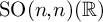 $\mathrm {SO}(n,n)({\mathbb R})$
, the four representations fuse two at a time to give a multiplicity free direct sum of two irreducible representations of
 $\mathrm {SO}(n,n)({\mathbb R}):$
 $$ \begin{align*}{\mathbb D_{\mu}}|_{\mathrm{SO}(n,n)({\mathbb R})} \ = \ \mathcal D_{\mu} \oplus \mathcal D_{^{\kappa_{2n}}\mu}, \end{align*} $$
where,
 $$ \begin{align*}\mathcal D_{\mu}|_{\mathrm{SO}(n,n)({\mathbb R})^{\circ}} \ := \ D_{\mu} \oplus {}^{s_{2n}}\!D_{\mu}, \ \ \text{and} \ \ \mathcal D_{{}^{\kappa_{2n}}\mu}|_{\mathrm{SO}(n,n)({\mathbb R})^{\circ}} \ := \ D_{{}^{\kappa_{2n}}\mu} \oplus {}^{s_{2n}}\!D_{{}^{\kappa_{2n}}\mu}. \end{align*} $$
For the finite-dimensional coefficient systems, let’s define
 $$ \begin{align*}\mathcal M_{\mu} \ := \ \mathrm{Ind}^{\mathrm{O}(n,n)({\mathbb R})}_{\mathrm{SO}(n,n)({\mathbb R})^{\circ}} (\mathcal N_{\mu}). \end{align*} $$
Restricting back to
 $\mathrm {SO}(n,n)({\mathbb R})^{\circ }$
, we get
 $$ \begin{align*}{\mathcal M}_{\mu}|_{\mathrm{SO}(n,n)({\mathbb R})^{\circ}} \ = \ {\mathcal N}_\mu \ \oplus \ {}^{\kappa_{2n}}{\mathcal N}_\mu \end{align*} $$
since
 ${\mathcal N}_\mu $
is an irreducible representation of
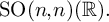 $\mathrm {SO}(n,n)({\mathbb R}).$
Now we observe that the cohomology
 $H^{q_0}({}^{\circ }{\mathfrak m}, {\mathfrak k};\, \mathbb D_{\mu } \otimes \mathcal M_{\mu })$
is a direct sum of four one-dimensional cohomology spaces:
 $$ \begin{align} H^{q_0}({}^{\circ}{\mathfrak m}, {\mathfrak k};\, D_{\mu} \otimes \mathcal N_{\mu} ) &\ \oplus \ H^{q_0}({}^{\circ}{\mathfrak m}, {\mathfrak k};\, {}^{s_{2n}}D_{\mu} \otimes \mathcal N_{\mu} ) \ \oplus \nonumber\\ &H^{q_0}({}^{\circ}{\mathfrak m}, {\mathfrak k};\,D_{{}^{\kappa_{2n}} \mu} \otimes \mathcal N_{^{\kappa_{2n}} \mu} ) \ \oplus \ H^{q_0}({}^{\circ}{\mathfrak m}, {\mathfrak k};\, {}^{s_{2n}} D_{^{\kappa_{2n}} \mu} \otimes \mathcal N_{^{\kappa_{2n}} \mu} ). \end{align} $$
2.2.8 The parameter of the discrete series representation
${\mathbb D_{\mu }}$
.

Let us recall some preliminaries on the Weil group of
 ${\mathbb R}$
:
 $W_{\mathbb R} = {\mathbb C}^\times \cup j\cdot {\mathbb C}^\times ,$
with
 $jzj^{-1} = \bar {z}$
for
 $z \in {\mathbb C}^\times .$
For an integer
 $\ell $
, define
 $\chi _\ell : {\mathbb C}^\times \to {\mathbb C}^\times $
as
 $\chi _\ell (z) = (z/\bar {z})^{\ell /2}$
or
 $\chi _\ell (re^{i\theta }) = e^{i\ell \theta }$
for
 $z = re^{i\theta } \in {\mathbb C}^\times .$
Define
 $I(\ell )$
to be the
 $2$
-dimensional induced representation
 $\mathrm {Ind}_{{\mathbb C}^\times }^{W_{\mathbb R}}(\chi _\ell ).$
Then
 $I(\ell ) \simeq I(-\ell )$
;
 $I(\ell )$
is irreducible if
 $\ell \neq 0$
;
 $I(0) = 1\!\!1 \oplus \mathrm {sgn}.$
Now, given
 $\mu $
as above with
 $\mu _1 \geq \cdots \geq \mu _{n-1} \geq |\mu _n|$
, put
 $$ \begin{align} \ell_1 = 2(\mu_1+n-1), \ \ \ell_2 = 2(\mu_2+n-2), \ \ \dots \ \ , \ \ell_{n-1} = 2(\mu_{n-1}+1), \ \ \ell_n = 2|\mu_n|. \end{align} $$
The Langlands parameter of
 ${\mathbb D_{\mu }}$
is the homomorphism
 $\varphi ({\mathbb D}_\mu ) : W_{\mathbb R} \to \mathrm {O}(2n)({\mathbb C})$
defined by
 $$ \begin{align*}{\mathbb C}^\times \ni z \mapsto (a_1,\dots,a_n,a_n^{-1},\dots,a_1^{-1}), \quad a_i = (z/\bar{z})^{\ell_i/2}; \quad j \mapsto J_{2n}. \end{align*} $$
This follows from from the very general [Reference Borel6, Ex. 10.5]; for the particular example at hand, see also [Reference Raghuram and Sarnobat30, Sect. 5.4]. The parameter is a direct sum of n induced representations:
 $$ \begin{align} \varphi({\mathbb D}_\mu) \ = \ I(\ell_1) \oplus \cdots \oplus I(\ell_{n-1}) \oplus I(\ell_n). \end{align} $$
Since
 $|\mu _n| \geq 1,$
each
 $\ell _i> 0,$
ensuring the irreducibility of the n-summands.
Let us add a comment that will be relevant in the next section. The parameter
 $\varphi ({\mathbb D}_\mu )$
thought of as a parameter of a representation of
 $\mathrm {GL}_{2n}({\mathbb R})$
, does not parametrise a cohomological representation. However, after any half-integral Tate twist – namely, for any
 $k \in {\mathbb Z}$
– the parameter
 $\varphi ({\mathbb D}_\mu ) \otimes |\ |^{(2k+1)/2}$
is indeed a parameter of a cohomological representation of
 $\mathrm {GL}_{2n}({\mathbb R}).$
See, for example, [Reference Raghuram27, 2.4.1.2].
2.2.9 Choice of a generic representation in L-packet.
We fix a Whittaker datum
 $\psi $
(i.e., a nontrivial additive character on the unipotent radical of the standard Borel subgroup of
 $^\circ M$
that is nontrivial on all simple root spaces). For a weight
 $\mu = (\mu ^v)_{v \in S_{\infty }}$
and an archimedean place v, consider the discrete series representation
 ${\mathbb D}_{\mu ^{v}} $
of
 $\mathrm {O}(n,n)({\mathbb R})$
as in Section 2.2.7. In the local L-packet (which is also a local A-packet in our context) of
 ${\mathbb D}_{\mu ^{v}} $
, there is a unique discrete series representation
 ${\mathbb D}^{\dagger }_{\mu ^{v}}$
which is
 $\psi _v$
-generic – that is, has a local Whittaker model with respect to
 $\psi _v$
. In Section 3.1, we consider this representation
 ${\mathbb D}^{\dagger }_{\mu ^{v}}$
while defining the strongly inner cohomology.
3 Strongly inner cohomology
We return to the global notations from Section 1. In particular, recall that
 ${}^{\circ }\!M_0 \cong \mathrm {O}(2n)/ F$
, and
 ${}^\circ \!M = \mathrm {Res}_{F/{\mathbb Q}}({}^\circ \!M_0).$
3.1 Strongly inner cohomology
Let
 $\mu \in X^*_+({}^\circ T \times E)$
be a dominant integral weight for
 ${}^\circ \!M.$
Recall that
 $\mu = (\mu ^\tau )_{\tau \in \mathrm {Hom}(F,E)},$
where
 $\mu ^\tau $
is an n-tuple of integers ordered as
 $\mu ^\tau _1 \geq \mu ^\tau _2 \geq \cdots \geq \mu ^\tau _{n-1} \geq |\mu ^\tau _n|.$
Define
 $$ \begin{align*}\mu_{\mathrm{min}} \ := \ \mathrm{min} \{ \, |\mu_n^{\tau} | \ : \ \tau \in \mathrm{Hom}(F,E) \}. \end{align*} $$
We henceforth assume that
 $\mu _{\mathrm {min}} \geq 1.$
For an open-compact subgroup
 ${}^\circ C_f$
of
 ${}^\circ \!M({\mathbb A}_f)$
, consider the sheaf
 $ \widetilde {\mathcal M}_{\mu ,E}$
on
 ${\mathcal S}^{{}^{\circ }\!M}_{{}^\circ C_f}.$
The inner cohomology
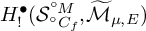 $H^{\bullet }_{!} (\mathcal S^{{}^\circ \! M}_{{}^{\circ }C_{f}}, \widetilde {\mathcal M}_{\mu ,E})$
is a module for the Hecke algebra
 ${\mathcal H}^{^{\circ }\!M}_{^{\circ }C_{f}} = \otimes _{v \notin S_\infty } {\mathcal H}^{^{\circ }\!M_{v}}_{^{\circ }C_{v}}$
over
 ${\mathbb Q}$
. Let S be a finite set of places containing
 $S_\infty $
, the ramified places of
 $F,$
and any place where
 ${}^{\circ }C_v$
is a proper subgroup of the maximal compact subgroup. Then,
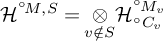 ${\mathcal H}^{{}^{\circ }\!M, S} = \mathbin {\mathop {\otimes }\limits _{v \notin S}} {\mathcal H}^{^{\circ }\!M_{v}}_{^{\circ }C_{v}}$
is a central subalgebra of
 ${\mathcal H}^{^{\circ }\!M}_{^{\circ }C_{f}}.$
We consider inner cohomology as a
 ${\mathcal H}^{^{\circ }\!M}_{^{\circ }C_{f}}$
-module. It is a general fact that inner cohomology is semi-simple as a Hecke module. Define
 $\mathrm {Coh}_{!}(^{\circ }\!M, \mu /E, {}^{\circ }C_{f})$
as the isomorphism classes of absolutely simple modules
 $\sigma _f$
over E (these are necessarily finite-dimensional E-vector spaces) which appear in
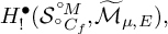 $H^{\bullet }_{!} (\mathcal S^{^{\circ }\!M}_{^{\circ }C_{f}}, \widetilde {\mathcal M}_{\mu ,E}),$
and inner cohomology is decomposed as the sum of such isotypic components
 $$ \begin{align*}H^{\bullet}_{!} (\mathcal S^{{}^{\circ}\!M}_{{}^{\circ}C_{f}}, \widetilde{\mathcal M}_{\mu,E}) \ = \ \bigoplus_{\sigma_f \in \mathrm{Coh}_{!}(M, \mu/E, {}^{\circ}C_{f})} H^{\bullet}_{!} (\mathcal S^{{}^{\circ}\!M}_{{}^{\circ}C_{f}}, \widetilde{\mathcal M}_{\mu,E}) (\sigma_f); \end{align*} $$
by taking E large enough we can guarantee that the full isotypic component of a particular
 $\sigma _f$
appears as a summand. Each
 $\sigma _f$
is isotypic as a
 ${\mathcal H}^{{}^{\circ }\!M, S}$
-module.
Towards defining the strongly inner spectrum
 $\mathrm {Coh}_{!!}(^{\circ }\!M, \mu /E, {}^{\circ }C_{f})$
, we fix once and for all a Whittaker datum
 $\psi $
for
 ${}^{\circ }\!M$
which is a nontrivial additive character on the unipotent radical of the standard Borel subgroup which is nontrivial on all simple root spaces. We also recall Arthur’s classification, as finessed by Atobe–Gan [Reference Atobe and Gan2], of the discrete (and hence cuspidal) spectrum of
 $^{\circ }\!M({\mathbb A}) = \mathrm {O}(2n)({\mathbb A}_F)$
in terms of automorphic representations of
 $\mathrm {GL}_{2n}({\mathbb A}_F)$
; the Arthur parameter of an irreducible automorphic representation
 $\varsigma $
appearing in the discrete spectrum of
 $^{\circ }\!M({\mathbb A})$
will be denoted
 $\Psi (\varsigma ).$
Let us also recall some notation from Section 1.6.1: an embedding
 $\iota : E \to {\mathbb C}$
gives an identification
 $X^*({}^\circ T \times E) \to X^*({}^\circ T \times {\mathbb C})$
that we denote
 $\mu \mapsto {}^\iota \mu .$
For
 $\mu = (\mu ^\tau )_{\tau : F \to E},$
identifying
 $\mathrm {Hom}(F,{\mathbb C})$
with
 $S_\infty ,$
and since
 $\iota $
induces a bijection
 $\mathrm {Hom}(F,E) \to \mathrm {Hom}(F,{\mathbb C}) = S_\infty $
via composition, for
 $v \in S_\infty $
, the v-th component
 ${}^\iota \mu _v$
is
 $\mu ^{\iota ^{-1}v}.$
Definition 25. Let
 $\mu \in X^*({}^\circ T \times E)$
be a dominant integral weight for
 ${}^\circ \!M.$
Assume that
 $\mu _{\mathrm {min}} \geq 1.$
For an open compact subgroup
 ${}^{\circ }C_f$
, the strongly inner spectrum of
 ${}^{\circ }\!M$
for the weight
 $\mu $
, denoted
 $\mathrm {Coh}_{!!}(^{\circ }\!M, \mu /E, {}^{\circ }C_f)$
, consists of those
 $\sigma _f \in \mathrm {Coh}_{!}(^{\circ }\!M, \mu /E, {}^{\circ }C_f)$
for which there exists an
 $\iota : E \rightarrow {\mathbb C}$
and a cuspidal automorphic representation
 $\varsigma $
of
 ${}^{\circ }\!M({\mathbb A}) = \mathrm {O}(2n)({\mathbb A}_F)$
such that
-
(i)
$\varsigma $
is globally generic with respect to
$\psi $
, -
(ii) the Arthur parameter
$\Psi (\varsigma )$
of
$\varsigma $
is a cuspidal representation of
$\mathrm {GL}_{2n}({\mathbb A}_F)$
, -
(iii) for all
$v \in S_{\infty },$
the v-th component
$\varsigma _v$
is
$\mathbb D^{\dagger }_{{}^\iota \!\mu _v}$
, the
$\psi _v$
-generic discrete series representation of
$\mathrm {O}(n,n)({\mathbb R})$
determined by
${}^\iota \!\mu _v$
(see Section 2.2.9), and -
(iv)
$\varsigma _f^{{}^{\circ }C_f} \cong \sigma _f \otimes _{E, \iota } {\mathbb C} $
as
${\mathcal H}^{^{\circ }\!M}_{^{\circ }C_{f}}$
-modules over
${\mathbb C}.$


Since the Arthur parameter
 $\Psi (\varsigma )$
is cuspidal, we know from [Reference Atobe and Gan2, Prop. 7.2] that
 $\varsigma $
appears in the cuspidal spectrum of
 ${}^\circ \!M$
with multiplicity one, and we let
 $V_\varsigma $
denote the representation space of
 $\varsigma $
inside of the space of cusp forms of
 ${}^\circ \!M$
. In the above definition, condition (i) pins down every local component
 $\varsigma _v$
in its local A-packet; however, there can be other cuspidal automorphic representations in the same global A-packet as
 $\varsigma $
and satisfying (iv). This is further elaborated upon in Section 3.3 below.
Define strongly inner cohomology as the space spanned by the isotypic components of strongly-inner Hecke-modules:
 $$ \begin{align*}H^{\bullet}_{!!}(\mathcal S^{^{\circ}\!M}_{^\circ C_{f}}, \widetilde {\mathcal M}_{\mu,E}) \ := \ \bigoplus_{\sigma_f \in \mathrm{Coh}_{!!}(^{\circ} \!M, \mu, {}^\circ C_{f})} H^{\bullet}_{!}(\mathcal S^{^{\circ}\!M}_{^\circ C_{f}}, \widetilde {\mathcal M}_{\mu,E}) (\sigma_f). \end{align*} $$
For brevity, denote
 $\mathrm {Coh}_{*}(^{\circ }\!M, \mu /E, {}^{\circ }C_{f})$
by
 $\mathrm {Coh}_{*}(^{\circ }\!M, \mu ),$
for
 $* \in \{!, !!\}$
, with the level structure
 ${}^{\circ }C_{f}$
and the field of coefficients E being understood.
The definition of strongly inner spectrum (and so also strongly inner cohomology) seemingly needs an embedding
 $\iota : E \to {\mathbb C}$
to invoke concepts of automorphic representation theory; however, we show independence of
 $\iota $
in the next subsection.
3.2 Galois equivariance
Let
 $\mu \in X^*({}^\circ T \times E)$
with
 $\mu _{\mathrm {min}} \geq 1,$
and
 $\sigma _f \in \mathrm {Coh}_{!!}(^{\circ }\!M, \mu ).$
For
 $\iota : E \to {\mathbb C}$
, let
 $\varsigma $
be the cuspidal automorphic representation of
 $^\circ \!M({\mathbb A}) = \mathrm {O}(2n)({\mathbb A}_F)$
as in Definition 25 above. The image of an
 $\iota : E \to {\mathbb C}$
lands in
 $\bar {{\mathbb Q}}$
, and we may further compose this with
 $\eta \in \mathrm {Gal}(\bar {{\mathbb Q}}/ {\mathbb Q}).$
We wish to understand what happens when we replace
 $\iota $
by
 $\eta \circ \iota $
; for this we need to be able to consider the Galois conjugate of a cuspidal representation of
 $\mathrm {O}(2n)({\mathbb A}_F)$
satisfying
 $(i)-(iii)$
of Definition 25. We show in this subsection that there is a cuspidal automorphic representation
 ${}^\eta \varsigma $
of
 $^\circ \!M({\mathbb A}) = \mathrm {O}(2n)({\mathbb A}_F)$
which is globally generic with respect to the same Whittaker datum
 $\psi ,$
and
 $({}^\eta \varsigma )_v = \varsigma _{\eta ^{-1}\circ v}$
for
 $v \in S_{\infty }$
, and whose Arthur parameter is
 $\Psi ({}^\eta \varsigma ) = {}^\eta (\Psi (\varsigma ) \otimes |\ |^{-1/2}) \otimes |\ |^{1/2}.$
Since
 $\varsigma $
is cuspidal and for
 $v \in S_\infty $
the local representation
 $\varsigma _v$
being a discrete series representation of
 $\mathrm {O}(n,n)({\mathbb R})$
, it follows that
 $\varsigma _f$
contributes to cuspidal cohomology (i.e.,
 $\varsigma _f$
appears as a Hecke-summand of
 $H^\bullet _{\mathrm {cusp}}(\mathcal S^{^{\circ }\!M}_{{}^\circ C_{f}}, \widetilde {\mathcal M}_{{}^\iota \mu ,{\mathbb C}})).$
(The reader is referred to [Reference Harder and Raghuram16, Sect. 3.2] for basics on cuspidal and square-integrable cohomology; although the reference is for general linear groups, the discussion in there applies mutatis mutandis to orthogonal groups.) But, cuspidal cohomology is contained inside inner cohomology which admits a natural rational structure since it is sheaf-theoretically defined, and so we may consider the effect of a Galois element on the latter. Furthermore, inner cohomology is contained in square-integrable cohomology which is captured by the discrete spectrum of
 $\mathrm {O}(2n)/F$
. This is summarised in the diagram:

that is, the
 $\eta $
-conjugate of
 $\varsigma _f,$
denoted
 ${}^\eta \varsigma _f,$
appears in inner-cohomology for the conjugated sheaf, and so also in square-integrable cohomology. Hence, there exists an automorphic representation
 $\delta $
that contributes to the global discrete spectrum of
 $\mathrm {O}(2n)/F$
such that
 $$ \begin{align*}\delta_f \ = \ {}^\eta\varsigma_f, \end{align*} $$
and furthermore,
 $\delta _\infty $
has nonvanishing relative Lie algebra cohomology with respect to the coefficient system
 ${\mathcal M}_{{}^{\eta \circ \iota }\mu ,{\mathbb C}},$
giving us the following equality of infinitesimal characters:
 $$ \begin{align*}\chi_{\delta_v} \ = \ \chi_{{\mathcal M}_{({}^{\eta\circ\iota}\mu)_v,{\mathbb C}}} \ = \ \chi_{{\mathcal M}_{({}^{\iota}\mu)_{\eta^{-1}v,{\mathbb C}}}} = \chi_{\varsigma_{\eta^{-1}v}}. \end{align*} $$
Since
 $\delta $
is in the discrete spectrum, we have its Arthur parameter
 $\Psi (\delta ).$
We claim that
 $\Psi (\delta )$
is a cuspidal representation of
 $\mathrm {GL}_{2n}({\mathbb A}_F).$
Now,
 $\Psi (\varsigma )$
is not of cohomological type on
 $\mathrm {GL}_{2n}({\mathbb A}_F)$
; however, as remarked in Section 2.2.8, after a half-integral Tate-twist, it becomes cohomological, and we know from Clozel [Reference Clozel11] that there is a Galois action on cohomological cuspidal representations of
 $\mathrm {GL}_{2n}({\mathbb A}_F)$
(i.e., we have the cuspidal representation
 ${}^\eta (\Psi (\varsigma ) \otimes |\ |^{-1/2})).$
For almost all v (where the local representations are unramified), we have
 $$ \begin{align*} \Psi( \delta)_v \ &= \ \Psi(\delta_v) \ = \ \Psi({}^\eta\varsigma_v) \\ &= \ \left({}^\eta(\Psi(\varsigma)_v \otimes |\ |^{-1/2})_v \otimes |\ |_v^{1/2}\right) \ = \ \left({}^\eta(\Psi(\varsigma) \otimes |\ |^{-1/2}) \otimes |\ |^{1/2}\right)_v, \end{align*} $$
where the third equality is an easy calculation with unramified principal series representations of
 $\mathrm {GL}_{2n}(F_v)$
. Hence, we have two Arthur parameters
 $\Psi _1 := \Psi ( \delta )$
and
 $\Psi _2 := {}^\eta (\Psi (\varsigma ) \otimes |\ |^{-1/2}) \otimes |\ |^{1/2}$
such that
 $\Psi _2$
cuspidal and
 $\Psi _{1,v} = \Psi _{2,v}$
for almost all v. Hence
 $\Psi _1 = \Psi _2,$
and in particular,
 $\Psi _1$
is also cuspidal. Let us record this as
 $$ \begin{align} \Psi( \delta) \ = \ {}^\eta(\Psi(\varsigma) \otimes |\ |^{-1/2}) \otimes |\ |^{1/2}. \end{align} $$
The Arthur parameter
 $\Psi ( \delta )$
for
 $\mathrm {O}(2n)$
is cuspidal, and so a partial symmetric square L-function,
 $L^S(s, \mathrm {Sym}^2, \Psi ( \delta )),$
has a pole at
 $s=1$
, and by the backward lifting (see Soudry [Reference Soudry36] and the references therein), there exists a unique globally
 $\psi $
-generic cuspidal representation
 $ \delta '$
of
 $\mathrm {O}(2n)$
whose local components transfer almost everywhere to the local components of
 $\Psi ( \delta ).$
Let
 $\Psi ( \delta ')$
be the Arthur parameter of
 $ \delta '$
. Once again, we have two Arthur parameters,
 $\Psi ( \delta )$
and
 $\Psi ( \delta '),$
that agree almost everywhere, and one of them is cuspidal, and hence so is the other, and they are equal; that is, we have
 $$ \begin{align} \Psi( \delta) \ = \ \Psi( \delta'). \end{align} $$
Fix
 $v \in S_\infty $
. Consider the local component
 $\delta ^{\prime }_v$
. We have
 $$ \begin{align*}\Psi(\delta^{\prime}_v) = \Psi(\delta')_v =\left(^{\eta}\!(\Psi(\varsigma) \otimes |\ |^{-1/2}) \otimes |\ |^{1/2}\right)_{v} = \Psi(\varsigma)_{\eta^{-1}v} = \Psi(\varsigma_{\eta^{-1}v}). \end{align*} $$
Hence,
 $\delta ^{\prime }_v$
and
 $\varsigma _{\eta ^{-1}v} = \mathbb {D}^{\dagger }_{{}^\iota \!\mu _{\eta ^{-1}v}}$
are in the same A-packet and indeed in the same L-packet; but
 $\delta ^{\prime }_v$
is also locally generic with respect to
 $\psi _v$
; hence,
 $\delta ^{\prime }_v = \mathbb {D}^{\dagger }_{{}^\iota \!\mu _{\eta ^{-1}v}} = \mathbb {D}^{\dagger }_{{}^{\eta \circ \iota }\!\mu _{v}}.$
Definition 28. Let
 $\varsigma $
be a cuspidal automorphic representation of
 $\mathrm {O}(2n)({\mathbb A}_F)$
that satisfies
 $(i)-(iii)$
of Definition 25. For
 $\eta \in \mathrm {Gal}(\bar {{\mathbb Q}}/ {\mathbb Q}),$
define the
 $\eta $
conjugate of
 $\varsigma $
, denoted
 ${}^\eta \varsigma $
, as the cuspidal representation
 $\delta '$
as above. Then
 ${}^\eta \varsigma $
satisfies
 $(i)-(iii)$
of Definition 25, where the highest weight for
 ${}^\eta \varsigma $
in
 $(iii)$
is the
 $\eta $
-conjugate of the highest weight for
 $\varsigma .$
The Arthur parameters are related by
 $$ \begin{align*}\Psi({}^\eta\varsigma) \ = \ {}^\eta(\Psi(\varsigma) \otimes |\ |^{-1/2}) \otimes |\ |^{1/2}. \end{align*} $$
Now we can see the independence of
 $\iota $
in Definition 25, in that if the conditions
 $(i)-(iv)$
hold for one embedding
 $\iota : E \to {\mathbb C}$
, then they hold for any embedding
 $\iota : E \to {\mathbb C}.$
Indeed, given some other
 $\iota ' : E \to {\mathbb C}$
, there is an
 $\eta \in \mathrm {Gal}(\bar {{\mathbb Q}}/ {\mathbb Q}),$
such that
 $\iota ' = \eta \circ \iota .$
Given a cuspidal representation
 $\varsigma $
attached to the data
 $\{\sigma _f, \iota \}$
, then the cuspidal representation
 ${}^\eta \varsigma $
is attached to the data
 $\{\sigma _f, \iota ' = \eta \circ \iota \}.$
3.3 The inner structure of an isotypic component of strongly inner cohomology
For
 $\sigma _f \in \mathrm {Coh}_{!!}(^\circ M, \mu )$
and
 $\iota : E \rightarrow {\mathbb C}$
, we wish to describe
 $$ \begin{align*}H^{\bullet}_{!!}(\mathcal S^{^{\circ}\!M}_{^\circ C_{f}}, \widetilde {\mathcal M}_{\mu,E}) (\sigma_f)\otimes_{E, \iota} {\mathbb C}. \end{align*} $$
Let
 ${\mathcal A}_2({}^\circ M) = {\mathcal A}_2\left( {}^{\circ } M({\mathbb Q}) \backslash {}^{\circ } M(\mathbb A) \right)$
denote the automorphic discrete spectrum of
 ${}^\circ M;$
see [Reference Atobe and Gan2, Sec. 6.7] for the definition of
 ${\mathcal A}_2({}^\circ M)$
. Inside,
 ${\mathcal A}_2({}^\circ M)$
is the cuspidal spectrum which we denote
 ${\mathcal A}_{\mathrm {cusp}}({}^\circ M) = {\mathcal A}_{\mathrm {cusp}} \left( {}^{\circ } M({\mathbb Q}) \backslash {}^{\circ } M(\mathbb A) \right).$
Consider the representation
 ${}^{\iota } \sigma : = \varsigma $
in Definition 25. There exist finitely many inequivalent cuspidal automorphic representations
 ${}^\iota \sigma = {}^\iota \sigma _{1},\ldots , {}^\iota \sigma _{l}$
of
 ${}^\circ \!M({\mathbb A})$
all having the same Arthur parameter as
 ${}^\iota \sigma ,$
and so appearing with multiplicity one in
 ${\mathcal A}_2({}^\circ M)$
([Reference Atobe and Gan2, Prop. 7.2]), indeed, appearing with multiplicity one in
 ${\mathcal A}_{\mathrm {cusp}}$
, and whose finite-parts are uniquely determined since
 ${}^\iota \sigma _{j,f}^{{}^\circ C_{f}} \cong \sigma _f \otimes _{E,\iota } {\mathbb C};$
however, for the archimedean components (i.e., for
 $v \in S_\infty $
),
 ${}^\iota \sigma _{j, v}$
can vary in the A-packet, or in this case, L-packet of
 $\varsigma _v$
which consists of discrete series representations determined by
 ${}^\iota \mu _v.$
For each
 $1 \leq j \leq l$
, we fix
 $$ \begin{align} \Phi_j \in \mathrm{Hom}_{(^\circ \mathfrak m({\mathbb R}), K^\circ_{{}^\circ\!M({\mathbb R})}) \times ^\circ M(\mathbb A_f)} \left( ^\iota \sigma_j, \ {\mathcal A}^2_{\mathrm{cusp}} \left( {}^{\circ} M({\mathbb Q}) \backslash ^{\circ} M(\mathbb A) \right) \right), \end{align} $$
which is unique up to scalars by the multiplicity-one property; denote
 $\Phi _j({}^\iota \sigma _j) = V_{{}^\iota \sigma _j}.$
The base-change to
 ${\mathbb C}$
via
 $\iota $
of the strongly-inner isotypic component of
 $\sigma _f$
takes the shape
 $$ \begin{align} H^{\bullet}_{!!}(\mathcal S^{^{\circ}\!M}_{^\circ C_{f}}, \widetilde {\mathcal M}_{\mu,E}) (\sigma_f)\otimes_{E, \iota} {\mathbb C} \ \ \cong \ \ \bigoplus_{j=1}^l H^\bullet({}^\circ \mathfrak m({\mathbb R}), K^\circ_{{}^\circ\!M({\mathbb R})}; \, V_{{}^\iota \sigma_j}^{{}^\circ C_{f}} \otimes {\mathcal M}_{{}^\iota\mu, {\mathbb C}}). \end{align} $$
Using the inverse of
 $\Phi _j$
in the j-th summand, we also have
 $$ \begin{align} H^{\bullet}_{!!}(\mathcal S^{^{\circ}\!M}_{^\circ C_{f}}, \widetilde {\mathcal M}_{\mu,E}) (\sigma_f)\otimes_{E, \iota} {\mathbb C} \ \cong \ \bigoplus_{j=1}^l H^\bullet({}^\circ \mathfrak m({\mathbb R}), K^\circ_{{}^\circ\!M({\mathbb R})}; \, {}^\iota \sigma_{j, \infty} \otimes {\mathcal M}_{{}^\iota\mu, {\mathbb C}}) \otimes {}^\iota \sigma_j^{{}^\circ C_{f}}. \end{align} $$
Note that for all
 $v \in S_{\infty }$
and
 $1 \leq j \leq l$
, we have
 $\Psi (^\iota \sigma _{j,v}) = \Psi ({\mathbb D}^{\dagger }_{\mu ^{v}})$
. From (31), it is clear that an absolutely simple Hecke-module represented by
 $\sigma _f$
, after base-change to
 ${\mathbb C}$
via
 $\iota $
, appears with finite-multiplicity in cuspidal cohomology. Later, in the context of the standard intertwining operator, we will simultaneously consider the cuspidal representations
 $^{\iota } \sigma _j$
and
 $^{\kappa _{2n}} { ^{\iota } \sigma _j}$
. Since
 $\kappa _{2n} \in {}^\circ M,$
we have
 $^{\iota } \sigma _j \cong {}^{\kappa _{2n}} { ^{\iota } \sigma _j}$
, and their representation spaces in the space of cusp forms are the same:
 $\Phi _j({}^{\iota } \sigma _j) = \Phi _j(^{\kappa _{2n}} { ^{\iota } \sigma _j}),$
or
 $V_{{}^{\iota } \sigma _j} = V_{{}^{\kappa _{2n}\iota } \sigma _j}.$
Also, for
 $1 \leq j,j' \leq l$
, if
 $j \neq j'$
, then the representations
 ${}^\iota \sigma _{j}$
and
 ${}^\iota \sigma _{j'}$
being inequivalent, implies that there is some
 $v \in S_\infty $
such that the local representations
 ${}^\iota \sigma _{j, v}$
and
 ${}^\iota \sigma _{j', v}$
are inequivalent. In particular,
 ${}^{\kappa _{2n} \iota } \sigma _j$
is not equivalent to
 ${}^{\iota } \sigma _{j'}.$
4 Critical set for L-functions for orthogonal groups
4.1 L-functions for orthogonal groups
Let
 $\mu \in X^*({}^\circ T \times E)$
be a dominant integral weight for
 ${}^\circ \!M$
with
 $\mu _{\mathrm {min}} \geq 1,$
and
 $\sigma _f \in \mathrm {Coh}_{!!}(^{\circ }M, \mu ).$
For
 $\iota : E \to {\mathbb C}$
, the cuspidal representation
 $\varsigma $
of Definition 25 will be henceforth denoted
 ${}^\iota \sigma .$
Let
 $\chi ^{\circ }$
be a finite order Hecke character of F taking values in
 $E,$
and d be an integer. Let
 $\chi $
stand for the algebraic Hecke character of F with values in E which gives a continuous homomorphism
 ${}^\iota \chi : F^\times \backslash {\mathbb A}_F^\times \to {\mathbb C}^\times $
of the form
 ${}^\iota \chi = {}^\iota \chi ^\circ \otimes |\ |^{-d}.$
The purpose of this section is to understand the critical set for the degree-
 $2n$
Langlands L-function
 $L(s, {}^\iota \chi \times {}^\iota \sigma ).$
For a place v of F, the local representation
 ${}^\iota \sigma _v$
is a representation of
 $\mathrm {O}(2n)(F_v)$
, and its restriction to
 $\mathrm {SO}(2n)(F_v)$
can be irreducible or a sum of two irreducible constituents that are mutually
 $\kappa _{2n}$
-conjugates since
 $\kappa _{2n} \in \mathrm {O}(2n)(F_v) \setminus \mathrm {SO}(2n)(F_v)$
. From Theorems 3.5, 3.6, 3.9 and 3.10 of Atobe–Gan [Reference Atobe and Gan2], we get an L-parameter for
 $\mathrm {O}(2n)(F_v)$
. Then we consider the degree-
 $2n$
local Langlands–Shahidi L-function
 $L_v(s, {}^\iota \chi _v \times {}^\iota \sigma _v)$
attached to the data
 ${}^\iota \chi _v$
and this L-parameter (corresponding to case (
 $D_{n,i}$
) of [Reference Shahidi33, App. A]). The global L-function is defined as a Euler product:
 $L(s, {}^\iota \chi \times {}^\iota \sigma ) = \prod _v L_v(s, {}^\iota \chi _v \times {}^\iota \sigma _v).$
The analytic properties of this L-function are well-understood by the Langlands–Shahidi machinery for which we refer the reader to Shahidi’s book [Reference Shahidi33].
4.2 Critical points for Rankin–Selberg L-functions for orthogonal groups
The infinite part of
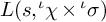 $L(s, {}^\iota \chi \times {}^\iota \sigma )$
is a product over archimedean places:
 $$\begin{align*}L_\infty(s, {}^\iota\chi \times {}^\iota\sigma) \ := \ \prod \limits_{v \in S_\infty} L(s, {}^\iota\chi_{v} \times {}^\iota\sigma_v). \end{align*}$$
An integer m is said to be a critical for
 $L(s, {}^\iota \chi \times {}^\iota \sigma )$
if both
 $$ \begin{align*}L_\infty(s, {}^\iota\chi \times {}^\iota\sigma) \ \ \mathrm{and}\ \ L_\infty(1-s, {}^\iota\chi^{-1} \times {}^\iota\sigma^{\mathsf{v}}) \end{align*} $$
are holomorphic at
 $s=m$
, where
 ${}^\iota \sigma ^{\mathsf {v}}$
is the contragredient of
 ${}^\iota \sigma .$
The purpose of this subsection is to determine all such critical integers.
Proposition 32. Let the notations be as in the first paragraph of Section 4.1. The critical set for the degree-
 $2n L$
-function
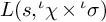 $L(s, {}^\iota \chi \times {}^\iota \sigma )$
is the contiguous set of
 $2\mu _{\min }$
integers:
 $$ \begin{align*}\left\{ 1+d-\mu_{\mathrm{min}}, ~ 2+d-\mu_{\mathrm{min}}, \ \dots \ , \ d+\mu_{\mathrm{min}}\right\}. \end{align*} $$
Since
 $\mu _{\mathrm {min}} \geq 1$
, there are at least two successive critical integers. The critical set is independent of
 $\iota $
.
Proof. For
 $v \in S_\infty $
, the local representation
 ${}^\iota \sigma _v$
is the discrete series representation
 ${\mathbb D}_{{}^\iota \!\mu ^{v}}$
of
 $\mathrm {O}(n,n)({\mathbb R}).$
As before, identifying
 $S_\infty $
with
 $\mathrm {Hom}(F,{\mathbb C})$
, we have
 ${}^\iota \!\mu ^{v} = \mu ^{\iota ^{-1}v}.$
For given v and
 $\iota ,$
let’s denote
 $\iota ^{-1}v$
by
 $\tau .$
Recall that
 $\mu ^\tau _1 \geq \cdots \geq \mu ^\tau _{n-1} \geq |\mu ^\tau _n| \geq 1.$
We know the Langlands parameter of
 ${}^\iota \sigma _v$
from (24). Also, the local component at v of the character
 $\chi $
may be expressed as
 $\chi _v = |\ |^{-d} \mathrm {sgn}^{\epsilon _v}$
with
 $\epsilon _v \in \{0,1\}.$
Recall that the
 $2$
-dimensional irreducible representation
 $I(\ell )$
of
 $W_{\mathbb R}$
is invariant under twisting by the sign character (i.e.,
 $I(\ell ) \otimes \mathrm {sgn} = I(\ell )).$
Recall also ([Reference Knapp22]) that the local L-factor attached to
 $I(\ell )$
is
 $2(2{\boldsymbol {\pi }})^{-(s+|\ell |/2)}\Gamma (s+|\ell |/2).$
Putting these together, and recalling
 $\ell ^\tau _j$
in terms of
 $\mu ^\tau _j$
from (23), we get the local L-factor at v as
 $$ \begin{align} L(s, {}^\iota\chi_{v} \times {}^\iota\sigma_v) &= \ L(s-d, {}^\iota\chi^\circ_{v} \times {}^\iota\sigma_v) \nonumber\\ & = 2^{n} \prod \limits_{j=1}^{n} (2 {\boldsymbol{\pi}})^{-(s-d+ |\mu_j^\tau| + n - j)} ~\Gamma(s-d+ |\mu_j^\tau| + n - j). \end{align} $$
To compute the critical integers, powers of
 $2$
and exponential terms – since they are holomorphic and nonvanishing everywhere – are not relevant. Ignoring such terms, we write
 $L(s, {}^\iota \chi _{v} \times {}^\iota \sigma _v) \approx \prod _{j=1}^{n} \Gamma (s-d+ |\mu _j^\tau | + n - j).$
Taking the product over
 $v \in S_\infty $
, which on the right-hand side will be taking the product over all
 $\tau : F \to E$
, we get
 $$ \begin{align*}L_\infty(s, {}^\iota\chi \times {}^\iota\sigma) \ \approx \ \prod_{\tau : F \to E} \, \prod_{j=1}^{n} \, \Gamma(s-d+ |\mu_j^\tau| + n - j). \end{align*} $$
Similarly, on the dual side we get
 $$ \begin{align*}L_\infty(1-s, {}^\iota\chi^{-1} \times {}^\iota\sigma^{\mathsf{v}}) \ \approx \ \prod_{\tau : F \to E} \, \prod_{j=1}^{n} \, \Gamma(1-s+d+ |\mu_j^\tau| + n - j). \end{align*} $$
We see that m is critical if and only if for all
 $\tau : F \to E$
and all
 $1 \leq j \leq n$
, both the conditions are satisfied:
-
•
$m-d+ | \mu _j^\tau |+ n - j \geq 1$
; -
•
$ 1 - m + d + |\mu _j^\tau | + n - j \geq 1$
.


Since
 $ \mu _1^\tau +n-1 \> \ \mu _2^\tau +n- 2 \ > \ \cdots \ > \ |\mu _n^\tau | \ \geq \ \mu _{\mathrm {min}},$
we see that the conditions are equivalent to
 $1 - \mu _{\mathrm {min}} \ \leq \ m-d \ \leq \ \mu _{\mathrm {min}}.$
We draw the following two easy corollaries of Proposition 32:
Corollary 34. The integers
 $-n$
and
 $1-n$
are critical for
 $L(s, {}^\iota \chi \times {}^\iota \sigma )$
if and only if
 $$ \begin{align*} 1 - \mu_{\mathrm{min}} \ \leq \ -(d+n) \ \leq \ \mu_{\mathrm{min}} - 1. \end{align*} $$
Corollary 35. If the inequalities in Corollary 34 hold, then
 $$ \begin{align*}\frac{L_\infty(-n, {}^\iota\chi \times {}^\iota\sigma)}{L_\infty(1-n, {}^\iota\chi \times {}^\iota\sigma)} \ \approx_{{\mathbb Q}^{\times}} \ {\boldsymbol{\pi}}^{n \textsf{r}_{\textsf{F}}}, \end{align*} $$
where
 $\approx _{{\mathbb Q}^{\times }}$
means equality up to a nonzero rational number.
Proof. Use the functional equation
 $\Gamma (s+1) = s \Gamma (s)$
and (33).
5 Kostant representatives and a combinatorial lemma
As in [Reference Harder and Raghuram16], we have a philosophically meaningful combinatorial lemma which says that the combinatorial condition in Corollary 34 that guarantees the successive integers
 $-n$
and
 $1-n$
to be critical for
 $L(s, {}^\iota \chi \times {}^\iota \sigma )$
is equivalent to the existence of some very special elements in the Weyl group of
 $G = \mathrm {Res}_{F/{\mathbb Q}}(\mathrm {O}(2n+2)/ F).$
This lemma will ultimately allow us to consider a particular induced representation in the cohomology of the Borel–Serre boundary of a locally symmetric space for G, thus permitting us to invoke the machinery of Eisenstein cohomology. Interestingly, the proof of the combinatorial lemma, which was challenging for general linear groups, is relatively easy in the situation of our orthogonal group G and the particular parabolic subgroup P we are interested in.
5.1 Weyl group
Recall our notation that
 $n = 2r$
, and
 $G_0 = \mathrm {O}(2n+2)/ F$
. The Weyl group
 $W_{G_0}$
is isomorphic to the subgroup of the group
 $\mathfrak {S}_{n+1} \rtimes ({\mathbb Z}/2{\mathbb Z})^{n+1}$
of signed permutations consisting of all signed permutations of
 $n+1$
symbols with an even number of sign changes. An element
 $w \in W_{G_0}$
permutes the
 $e_j$
’s according to the corresponding signed permutation.
Recall the maximal parabolic subgroup
 $P_0$
of
 $G_0$
from Section 1.7 corresponding to deleting the simple root
 $\alpha _0.$
Let
 $w_{P_{0}} $
be the unique element of
 $W_{G_0}$
such that
 $w_{{P_{0}}}( \Pi _{G_{0}} \setminus \{ \alpha _0\}) \subset \Pi _{G_{0}}$
and
 $w_{P_0}( \alpha _{0}) < 0$
. Observe that
 ${P_{0}}$
is self associate, and we have
 $$ \begin{align*}w_{{P_{0}}}(\Pi_{G_{0}} \setminus \{ \alpha_0 \}) = \Pi_{G_{0}} \setminus \{ \alpha_0\} ~ \text{and}~w_{P_{0}}(\Delta_{U{_{0}}}) = - \Delta_{U_{0}}, \end{align*} $$
where
 $\Delta _{U_{0}}$
is the set of positive roots with root spaces in
 $\mathfrak {u}_{P_0} = \mathrm {Lie}(U_{P_0}).$
The element
 $w_{P_0}$
is the signed permutation:
 $$ \begin{align*}e_0 \mapsto -e_0, \quad e_i \mapsto e_i \ \ \mathrm{for} \ \ 1 \leq i \leq n-1, \quad e_n \mapsto -e_n. \end{align*} $$
The element
 $w_{P_0}$
can be factorised as a product in terms of the simple reflections
 $\mathsf {s}_{\alpha _{j}}$
as
 $$ \begin{align} w_{P _{0}} \ = \ \mathsf{s}_{\alpha_{0}} ~\mathsf{s}_{\alpha_{1}} ~\cdots ~ \mathsf{s}_{\alpha_{n-3}} ~ \mathsf{s}_{\alpha_{n-2}} ~\mathsf{s}_{\alpha_{n}} ~\mathsf{s}_{\alpha_{n-1}} \mathsf{s}_{\alpha_{n-2}} ~\cdots~ \mathsf{s}_{\alpha_{1}} ~\mathsf{s}_{\alpha_{0}}. \end{align} $$
The length of
 $w_{P _{0}}$
is
 $l(w_{P _{0}}) = 2n = \dim (U_{P_0}).$
The Weyl group of
 $G \times E$
factors as a product
 $$ \begin{align*}W_{G \times E} \ = \ \prod \limits_{\tau: F \rightarrow E} \, W_{G_0 \times_{F, \tau} E}, \end{align*} $$
where each
 $W_{G_0 \times _{F, \tau } E}$
is isomorphic to
 $W_{G_{0}}$
. Sometimes, we abbreviate
 $W_{G_0 \times _{F, \tau } E}$
as
 $W^\tau .$
The element
 $w_P \in W_{G \times E}$
is
 $(w_{P_0}^\tau )_{\tau : F \to E}$
, where each
 $w_{P_0}^\tau $
is the copy of
 $w_{P_0}$
in
 $W_{G_0 \times _{F, \tau } E}.$
The length of
 $w_{P}$
is
 $l(w_{P}) = 2n \mathsf {r}_F = \dim (U_P).$
The twisted action of
 $w \in W_{G \times E}$
on
 $\lambda \in X^{\ast }(T \times E)$
is given by
 $w \cdot \lambda : = (w^{\tau } \cdot \lambda ^\tau )_{\tau : F \rightarrow E},$
where
 $$ \begin{align*}w^{\tau} \cdot \lambda^{\tau} \ := \ w^{\tau} (\lambda^{\tau} + {\boldsymbol{\rho}}_{G^{\tau}_{0}}) - {\boldsymbol{\rho}}_{G^{\tau}_0}. \end{align*} $$
5.2 Kostant representatives
Let
 $\Pi _{M_{P_{0}}}$
denote the set of simple roots of the Levi quotient
 $M_{P_0}$
of
 $P_0.$
The set of Kostant representatives in
 $W_{G_0}$
corresponding to the parabolic subgroup
 $P_0$
is defined as
 $$ \begin{align*}W^{P_{0}} \ := \ \{ w \in W_{G_0} \ : \ w^{-1} \alpha> 0 \ \ \forall \alpha \in \Pi_{M_{P_{0}}} \}. \end{align*} $$
Now define the set of Kostant representatives in
 $W_{G \times E}$
corresponding to the parabolic subgroup P as
 $$ \begin{align*}W^{P} \ = \ \left\{ w = (w^{\tau}) \ : \ w^{\tau} \in {W^{\tau}}^{P_{0}^{\tau}} \right\}. \end{align*} $$
If
 $w_0 \in W^{P_{0}}$
, then for its length, we have
 $0 \leq \ell (w_0) \leq \dim (U_{P_0})$
, and hence, for
 $w \in W^P$
, we have
 $0 \leq \ell (w) \leq \dim (U_{P}).$
Recall that
 $\dim (U_{P_0}) = 2n$
is even.
Definition 37. We say
 $w_0 \in W^{P_{0}}$
is balanced if
 $\ell (w_0) = \tfrac {1}{2} \dim (U_{P_0}),$
and we say
 $w = (w^{\tau }) \in W^P$
is balanced if each
 $w^\tau $
is balanced (i.e.,
 $\ell (w^{\tau }) = \tfrac {1}{2} \dim (U_{P_{0}^{\tau }})$
for each
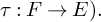 $\tau : F \to E).$
In the self-associate case of our parabolic subgroup P, a couple of self-bijections of
 $W^P$
with complementary lengths will be important. We record these in the following two propositions. (See Lemma 5.6 and Lemma 5.7 of [Reference Harder and Raghuram16], the proofs of which are totally general.)
Proposition 38. The map
 $w \mapsto w': = w_P\,w$
defines a bijection
 $W^P \rightarrow W^P$
such that
 $\ell (w) + \ell (w') = \mathrm {dim}(U_{P}).$
Hence, w is balanced if and only if
 $w'$
is balanced.
Let
 $w_{G_0}$
be the element of
 $W_{G_0}$
with longest length. As a signed permutation, it is
 $$ \begin{align*}e_i \mapsto -e_i \ \ \mathrm{for} \ \ 0 \leq i \leq n-1, \ \ \mathrm{and} \quad e_n \mapsto e_n. \end{align*} $$
(Since n is even, we have an even number of sign changes.) The element
 $w_G \in W_{G \times E}$
is
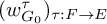 $(w_{G_0}^\tau )_{\tau : F \to E}$
, where each
 $w_{G_0}^\tau $
is the copy of
 $w_{G_0}$
in
 $W_{G_0 \times _{F, \tau } E}.$
Similarly, let
 $w_{M_0}$
be the element of
 $W_{M_{P_0}}$
of longest length which is given by
 $$ \begin{align*}e_i \mapsto -e_i \quad \mathrm{for} \ 1 \leq i \leq n. \end{align*} $$
We have
 $w_{M} = (w_{M_0}^\tau )_{\tau : F \to E},$
where
 $w_{M_0}^\tau $
is the copy of
 $w_{M_0}$
in
 $W_{G_0 \times _{F, \tau } E}.$
Proposition 39. The map
 $W^P \rightarrow W^P$
defined by
 $w \mapsto w^{\mathsf {v}}: = w_{M} \, w \, w_G$
is a bijection such that
 $\ell (w) + \ell (w^{\mathsf {v}}) = \dim (U_P).$
Hence, w is balanced if and only if
 $w^{\mathsf {v}}$
is balanced.
In the set of Kostant representatives
 $W^{P_0}$
, one can check that there are only two balanced elements
 $w^+$
and
 $w^{-}$
which are described below:
 $$ \begin{align*} \begin{aligned} &w^+: \quad e_i \mapsto e_{i+1} \quad \mathrm{for} \ 0 \leq i \leq n-1, \quad e_n \mapsto e_0; \\ &w^-: \quad e_i \mapsto e_{i+1} \quad \mathrm{for} \ 0 \leq i \leq n-2, \quad e_{n-1} \mapsto -e_n, \quad e_n \mapsto -e_0. \end{aligned} \end{align*} $$
It follows using the definitions of the self-bijections in the propositions above that
 $$ \begin{align*} \begin{aligned} & w^+{}' = w^-, \quad w^-{}' = w^+; \\ & w^+{}^{\mathsf{v}} = w^+, \quad w^-{}^{\mathsf{v}} = w^-. \end{aligned} \end{align*} $$
5.3 A Combinatorial lemma
Let the notations be as in the first paragraph of Section 4.1. The weight
 $\mu = (\mu ^\tau )_{\tau : F \to E} \in X^*_+({}^\circ \!T \times E)$
and the integer d give a weight
 $de_0 + \mu \in X^*(T\times E)$
whose
 $\tau $
-component is
 $de_0 + \mu ^\tau .$
Note that
 $de_0 + \mu $
need not be dominant as a weight for
 $G.$
Lemma 40 (Combinatorial lemma).
With notations as above, the following are equivalent:
-
(i)
$-n$
and
$1-n$
are critical points for the L-function
$L(s, {}^\iota \chi \times {}^\iota \sigma )$
; -
(ii)
$1 - \mu _{\mathrm {min}} \ \leq \ -(n+d) \ \leq \ \mu _{\mathrm {min}} - 1;$
-
(iii) There exists a balanced Kostant representative
$w \in W^P$
such that
$w^{-1} \cdot (de_0 + \mu )$
is a dominant integral weight for
$G.$


Proof. The equivalence
 $(i) \iff (ii)$
is exactly Corollary 34. It suffices to prove
 $(ii) \iff (iii)$
.
Suppose
 $(ii)$
holds. A calculation shows that
 $$ \begin{align*} \begin{aligned} (w^{+})^{-1} \cdot (de_0 + \mu^{\tau}) = (\mu_1^{\tau} -1)~ e_0 + \ldots + (\mu_n ^{\tau}- 1)~ e_{n-1} + (d+n)~ e_n, \\ (w^{-})^{-1} \cdot (de_0 + \mu^{\tau}) = (\mu^{\tau}_1 -1)~ e_0 + \ldots + (-\mu^{\tau}_n - 1)~ e_{n-1} - (d+n)~ e_n. \end{aligned} \end{align*} $$
For
 $\tau : F \to E$
, if
 $\mu ^{\tau }_n \geq 1$
, then take
 $w^{\tau } = w^+$
, and if
 $\mu ^\tau _n \leq -1$
, then take
 $w^{\tau } = w^-$
. Now put
 $w = (w^\tau )_{\tau : F \to E}$
, which is a balanced element of
 $W^P.$
For each
 $\tau $
, observe that
 $(w^\tau )^{-1} \cdot (de_0 + \mu ^\tau )$
is dominant; indeed, if
 $\mu ^{\tau }_n \geq 1$
, then
 $(ii)$
implies that
 $\mu _n ^{\tau }- 1 \geq |d+n|$
, rendering
 $(w^{+})^{-1} \cdot (de_0 + \mu ^{\tau })$
dominant, and if
 $\mu ^{\tau }_n \leq -1$
, then
 $(ii)$
implies that
 $-\mu _n ^{\tau }- 1 \geq |d+n|$
, rendering
 $(w^{-})^{-1} \cdot (de_0 + \mu ^{\tau })$
dominant. Hence
 $(iii)$
.
Conversely, if
 $(iii)$
holds for some balanced element w of
 $W^P,$
then for a given
 $\tau ,$
the above formulae tell us that the sign of
 $\mu _n^\tau $
determines if
 $w^\tau $
is
 $w^+$
or
 $w^-,$
and furthermore, that
 $1- |\mu ^{\tau }_n| \leq -(n+d) \leq |\mu ^{\tau }_n|-1.$
But this is true for all
 $\tau .$
Hence,
 $(ii)$
.
5.4 Consequences of the combinatorial lemma
Under the notations and conditions imposed by the Combinatorial Lemma (Lemma 40), let’s record some consequences on the effect of Kostant representatives related to
 $w,$
such as
 $w'$
,
 $w^{\mathsf {v}}$
and
 $w^{\mathsf {v}}{}'$
(see Proposition 38 and Proposition 39), on some weights related to
 $\lambda : = w^{-1} \cdot (de_0 + \mu ).$
For
 $\mu \in X^*({}^\circ \!T \times E)$
, define
 $\mu ^{\mathsf {v}} := -w_{M_{P}} \mu .$
Observe that
 $\mu ^{\mathsf {v}} = \mu ,$
reflecting the fact that the representation
 ${\mathcal M}_{\mu ,E}$
is self-dual. Similarly, for
 $\lambda \in X^*(T \times E)$
, define
 $\lambda ^{\mathsf {v}} : = -w_{G} \lambda .$
When
 $\lambda $
is dominant-integral, then
 $\lambda ^{\mathsf {v}}$
is the the highest weight of the dual of
 ${\mathcal M}_{\lambda ,E}$
. We omit the proof of the following proposition which is a straightforward calculation. The information in this proposition will be relevant when we deal with Poincaré duality for the cohomology of the Borel–Serre boundary.
Proposition 41. Under the notations and conditions of Lemma 40, for
 $\lambda : = w^{-1} \cdot (de_0 + \mu ),$
we have
-
(1)
$w' \cdot \lambda \ = \ (-d -2n) e_0 + ~^{\kappa _{2n}} \mu $
. -
(2)
$ w^{\mathsf {v}} \cdot \lambda ^{\mathsf {v}} \ = \ (-d-2n) e_0 + \mu ^{\mathsf {v}} \ = \ (-d-2n) e_0 + \mu $
. -
(3)
$w^{\mathsf {v}}{}' \cdot \lambda ^{\mathsf {v}} \ = \ d e_0 + {}^{\kappa _{2n}}\!\mu ^{\mathsf {v}} \ = \ d e_0 + {}^{\kappa _{2n}}\!\mu $
.


6 Arithmetic of intertwining operators
We continue with our global notations as in the first paragraph of Section 4.1. Since the embedding
 $\iota : E \to {\mathbb C}$
will be fixed throughout this section, we will allow ourselves, only for this section, an abuse of notation that will not cause any confusion: denote the cuspidal automorphic representation
 ${}^\iota \sigma $
of
 ${}^\circ \!M({\mathbb A}) = {}^\circ \!M_0({\mathbb A}_F) = \mathrm {O}(2n)({\mathbb A}_F)$
simply by
 $\sigma $
, and similarly, denote the Hecke character
 ${}^\iota \chi $
of F simply as
 $\chi $
which is of the form
 $ \chi ^\circ \otimes |\ |^{-d}$
for a finite-order character
 $\chi ^\circ .$
6.1 Induced representations
We begin by recalling the induced representations as set up in the Langlands–Shahidi machinery [Reference Shahidi33]. Recall that the Levi-quotient
 $M_0 = M_{P_0}$
of the maximal parabolic subgroup
 $P_0$
of
 $G_0$
corresponding to deleting the simple root
 $\alpha _0 = e_0 - e_1$
is explicitly given by
 $$ \begin{align*}M_0 = \left\{ m_{x,g} = \left(\begin{matrix} x & & \\ & g & \\ & & x^{-1}\end{matrix}\right) \ : \ x \in A_0 = \mathrm{GL}_1/F, \ \ g \in {}^{\circ}\!M_0 = \mathrm{O}(2n)/F \right\} = A_0 \times {}^\circ\!M_0. \end{align*} $$
We have the dual of the real Lie algebra
 ${\mathfrak a}^* = X^*(M_0) \otimes {\mathbb R} = X^*(A_0) \otimes {\mathbb R} = {\mathbb R} \, e_0.$
The set of roots whose root spaces appear in
 $U_{P_0}$
is
 $\{e_0 \pm e_i : 1 \leq i \leq n\}$
, and half their sum is
 ${\boldsymbol {\rho }}_{P_0} = n\, e_0.$
We have
 $\langle {\boldsymbol {\rho }}_{P_0}, \alpha _0 \rangle = 2 ({\boldsymbol {\rho }}_{P_0}, \alpha _0)/(\alpha _0, \alpha _0) = n.$
The fundamental weight
 $\tilde {\alpha }$
corresponding to
 $\alpha _0$
is
 $$ \begin{align*}\tilde{\alpha} \ = \ \langle {\boldsymbol{\rho}}_{P_0}, \alpha_0 \rangle^{-1} {\boldsymbol{\rho}}_{P_0} \ = \ e_0. \end{align*} $$
For any place v of F, the modular character
 $\delta _{P_0}$
at v given by the adjoint action of
 $M_{P_0}(F_v)$
on
 $U_{P_0}(F_v)$
is
 $\delta _{P_0, v}(m_{x,g}) = |x|_v^{2n}.$
At an adèlic level, it has the same form:
 $\delta _{P_0}(m_{x,g}) = |x|^{2n}.$
Hence,
 $\delta _{P_0}^{1/2} = |{\boldsymbol {\rho }}_{P_0}|.$
For
 $s \in {\mathbb C}$
, in the Langlands–Shahidi method, we start with the induced representation
 $I(s\tilde {\alpha }, \chi \otimes \sigma ),$
which we will denote simply as
 $I(s, \chi \times \sigma ),$
consisting of all smooth functions
 $f: G_0({\mathbb A}_F) \longrightarrow V_{\sigma }$
such that
 $$ \begin{align*}f(m_{x,g}uh ) \ = \ |x|^{n+s} \, \chi(x) \, \sigma(g) \, f(h), \end{align*} $$
for all
 $m_{x,g} \in M_{P_0}({\mathbb A}_F), \ u \in U_{P_0}({\mathbb A}_F), \ h \in G_0({\mathbb A}_F).$
In terms of normalised parabolically induced representations, we have
 $$ \begin{align*}I(s, \chi \times \sigma) \ = \ \mathrm{Ind}_{P({\mathbb A})}^{G({\mathbb A})} \left(\chi[s] \times \sigma \right), \end{align*} $$
where
 $\chi [s] = \chi \otimes |\ |^s.$
In terms of algebraically (un-normalised) parabolically induced representations, we have
 $$ \begin{align*}I(s, \chi \times \sigma) \ = \ {}^{\mathrm{a}}\mathrm{Ind}_{P({\mathbb A})}^{G({\mathbb A})} \left(\chi[s+n] \times \sigma \right). \end{align*} $$
In particular, observe that
 $$ \begin{align*}I(s, \chi \times \sigma)|_{s = -n} \ = \ {}^{\mathrm{a}}\mathrm{Ind}_{P({\mathbb A})}^{G({\mathbb A})} \left(\chi \times \sigma \right). \end{align*} $$
We designate
 $s = s_0 = -n$
as our point of evaluation. The algebraic induction works well for cohomological purposes, whereas the analytic theory of Langlands–Shahidi L-functions works well with normalised induction. In the arithmetic theory of L-functions, it is a necessary evil to go back and forth between these two forms of induction.
6.2 The standard intertwining operator
The weyl group element
 $w_{P_{0}}$
defined in Section 5.1 is realised by conjugation by the matrix in
 $\mathrm {O}(2n+2)$
:
 $$ \begin{align*}\tilde{w}_{P_0} \ = \ \begin{pmatrix} & & & & 1 \\ & I_{n-1} & & & \\ & & J_2 & & \\ & & & I_{n-1} & \\ 1 & & & & \end{pmatrix}. \end{align*} $$
We will denote
 $\tilde {w}_{P_0} $
simply as
 $w_{P_0}$
itself. The conjugation action of
 $w_{P_0}$
on the inducing representation is given by
 $w_{P_0}(\chi [s] \times \sigma ) = \chi ^{-1}[-s] \times {}^{\kappa _{2n}} \sigma ,$
where the element
 $\kappa _{2n}$
was defined in (20). The standard global intertwining operator
 $$ \begin{align*}T_{\mathrm{st}}(s, w_{P_0}, \chi \times \sigma) \ : \ I(s, \chi \times \sigma) \ \longrightarrow \ I(-s, \chi^{-1} \times {}^{\kappa_{2n}} \sigma) \end{align*} $$
is defined by the integral
 $$ \begin{align*}T_{\mathrm{st}}(s, w_{P_0}, \chi \times \sigma)(f)(g) \ = \ \int \limits_{U_P({\mathbb A})} f(w_{P_0}^{-1} \, u\, g) \, du. \end{align*} $$
We will denote
 $T_{\mathrm {st}}(s, w_{P_0}, \chi \times \sigma )$
simply by
 $T_{\mathrm {st}}(s, w_{P_0})$
or even just
 $T_{\mathrm {st}}(s).$
The intertwining operator
 $T_{\mathrm {st}}(s)$
is a product of local intertwining operators
 $$ \begin{align*}T_{\mathrm{st}}(s) \ = \ \otimes^{\prime}_v \, T_{\mathrm{st}, v}(s), \end{align*} $$
where the local operators are defined by analogous local integrals for each place
 $v $
of F. The global measure
 $du$
on
 $U_P({\mathbb A}) = U_{P_0}({\mathbb A}_F)$
is a product over the coordinates of
 $U_{P_0}$
of the additive measure
 $dx$
on
 ${\mathbb A}_F$
, which in turn is a product
 $\prod _v dx_v$
of local additive measures
 $dx_v$
on
 $F_v^+$
; for a finite place v, we normalise
 $dx_v$
by
 $\mathrm {vol}({\mathcal O}_v) = 1$
, where
 ${\mathcal O}_v$
is the ring of integers of
 $F_v$
, and for an archimedean v, we take
 $dx_v$
as the Lebesgue measure on
 ${\mathbb R}.$
6.3 Local intertwining operators at a non-archimedean place: unramified case
Since we are dealing with an algebraically disconnected group
 $\mathrm {O}(2n)$
and not the connected algebraic group
 $\mathrm {SO}(2n)$
, some brief comments are in order on local unramified representations. The reader is referred to [Reference Atobe and Gan2, Sect. 2.3] for further details. For a finite place v of F, let
 ${\mathcal O}_v$
be the ring of integers of
 $F_v$
,
 $\varpi _v$
a uniformizer, and
 $q_v$
the cardinality of the residue field
 ${\mathcal O}_v/\varpi _v{\mathcal O}_v$
. Assume that v is such that
 $\chi _v$
and
 $\sigma _v$
are unramified. The orthogonal space we consider is
 $F^{2n}$
with a basis
 $\{w_1,\dots ,w_n, w_n^*,\dots ,w_1^*\}$
, and the nondegenerate symmetric bilinear form on
 $F^{2n}$
is represented by the matrix
 $J_{2n}$
with respect to this basis. Consider the
 ${\mathcal O}_v$
-lattice
 $L_v$
in
 $F^{2n} \otimes F_v = F_v^{2n}$
spanned by this basis:
 $$ \begin{align*}L_v \ = \ {\mathcal O}_v w_1 \oplus \cdots \oplus {\mathcal O}_v w_n \oplus {\mathcal O}_v w_n^* \oplus \cdots \oplus {\mathcal O}_v w_1^*. \end{align*} $$
Let
 $K_v$
be the subgroup of
 $\mathrm {O}(2n)(F_v)$
that stabilizes the lattice
 $L_v$
. Then
 $K_v$
is a maximal compact subgroup of
 $\mathrm {O}(2n)(F_v)$
. We have
 $K_v = K_v^1 \ltimes \langle \kappa _{2n} \rangle $
, where
 $K_v^1 = K_v \cap \mathrm {SO}(2n)(F_v)$
is a maximal compact subgroup of
 $\mathrm {SO}(2n)(F_v)$
. We say an irreducible admissible representation
 $\pi $
(resp.,
 $\pi _1$
) of
 $\mathrm {O}(2n)(F_v)$
(resp.,
 $\mathrm {SO}(2n)(F_v)$
) is unramified if
 $\pi $
(resp.,
 $\pi _1$
) has a nonzero vector fixed by
 $K_v$
(resp.,
 $K_v^1$
). It is known in this case that
 $\dim (\pi ^{K_v}) = \dim (\pi _1^{K_v^1}) = 1.$
The nonzero vector fixed by
 $K_v$
(or
 $K_v^1$
) will be called a spherical vector. (The reader specifically interested in comparing our notations with [Reference Atobe and Gan2] will note that our
 $2n$
-dimensional orthogonal space is the
 $V_{2n}$
on p. 358 of loc.cit. with
 $c = d = 1.$
)
The relation between the local intertwining operator at a finite unramified place and local L-functions is a famous calculation of Langlands that generalises the classical Gindikin–Karpelevich formula. This is a well-known part of the Langlands–Shahidi machinery; we will briefly review the results as applied to our situation and refer the reader to Shahidi’s book [Reference Shahidi33] for more details. Let
 $f_v^\circ $
denote the normalised spherical vector in the local induced representation
 $I_v(s, \chi _v \times \sigma _v)$
– normalised by taking the value
 $1$
on the identity element. Similarly, let
 $\tilde {f}_v^\circ $
denote the normalised spherical vector in
 $I_v(-s, \chi _v^{-1} \times {}^{\kappa _{2n}}\sigma _v)$
. Then
 $$ \begin{align} T_{\mathrm{st}, v}(s)(f_v^\circ) = \frac{L_v(s, \chi_v \times \sigma_v)}{L_v(1+s, \chi_v \times \sigma_v)} \ \tilde{f}_v^\circ. \end{align} $$
Let us recall the local L-factor
 $L_v(s, \chi _v \times \sigma _v)$
. Suppose
 $\mathrm {diag}(\vartheta _{v,1},\dots ,\vartheta _{v,n}, \vartheta _{v,n}^{-1}, \dots , \vartheta _{v,1}^{-1}) \in \mathrm {O}(2n)({\mathbb C})$
represents the Satake parameter of
 $\sigma _v$
, and
 $\vartheta _v = \chi _v(\varpi _v)$
that of
 $\chi _v$
. Then we have
 $$ \begin{align*}L_v(s, \chi_v \times \sigma_v) \ = \ \prod_{j=1}^n \left((1- \vartheta_v \, \vartheta_{v,j}\, q_v^{-s}) (1- \vartheta_v\, \vartheta_{v,j}^{-1}\, q_v^{-s}) \right)^{-1}. \end{align*} $$
A subtle point to appreciate is the manner in which the complex variable s is inserted in the induced representation, via the
 $s\tilde {\alpha }$
, which has a bearing on the precise form of (42).
6.4 Langlands’s constant term theorem
So far in our discussion of intertwining operators, we did not talk about convergence issues. As is well-known, convergence is guaranteed in some half-plane, and one has a meromorphic continuation to all
 $s \in {\mathbb C}.$
The holomorphy of the intertwining operator, Eisenstein series, and holomorphy of global (partial) L-functions are all related by Langlands’s constant term theorem that we now recall. A section
 $f \in I(s, \chi \times \sigma )$
can be identified with the function
 $\underline {g} \mapsto f(\underline {g})(\underline {1})$
on
 $G({\mathbb A})$
, letting us embed
 The Eisenstein series associated to f is defined via Eisenstein summation for
 $\Re (s) \gg 0$
:
 $$ \begin{align*}\mathrm{Eis}_{P} (s,f)(\underline{g}) \ = \ \sum \limits_{\gamma \in P({\mathbb Q}) \backslash G({\mathbb Q})} f(\gamma \, \underline{g}), \end{align*} $$
giving us a map
 $ \mathrm {Eis}_{P}(s,-) : \mathcal {C}^{\infty }(P({\mathbb Q}) \backslash G({\mathbb A})) \rightarrow \mathcal {C}^{\infty }(G({\mathbb Q}) \backslash G({\mathbb A})). $
Next, we can take the constant term along P for
 $\phi \in \mathcal {C}^{\infty }(G({\mathbb Q}) \backslash G({\mathbb A}))$
defined by
 $$ \begin{align*}\mathcal F_P(\phi)(\underline{g}) = \int \limits_{U_P({\mathbb Q}) \backslash U_P({\mathbb A})} \phi(\underline u \, \underline g) \, d\underline u, \end{align*} $$
giving us a map
 $ \mathcal F_{P} : \mathcal {C}^{\infty }(G({\mathbb Q}) \backslash G({\mathbb A})) \to \mathcal {C}^{\infty }(P({\mathbb Q}) \backslash G({\mathbb A})). $
Langlands’s theorem gives a relation between the intertwining operator
 $T_{\mathrm {st}}(s)$
, the Eisenstein map
 $\mathrm {Eis}_{P}(s,-),$
and the constant term map
 $\mathcal {F}_{P}.$
The reader will note that the parabolic P under consideration is self-associate.
Theorem 43 (Langlands).
For
 $f \in I(s, \chi \times \sigma )$
we have
 $$ \begin{align*}\mathcal F_{P} ( \mathrm{Eis}_{P}(s,f)) = f + T_{st}(s)(f).\end{align*} $$
The program enunciated by Harder [Reference Harder15], and continued in [Reference Harder and Raghuram16], on Eisenstein cohomology and special values of L-functions, hinges on giving a cohomological interpretation to Langlands’s theorem.
6.5 Holomorphy of Eisenstein series at point of evaluation
We will be specifically interested in Langlands’s constant term theorem at our point of evaluation
 $s = -n.$
For this, we will need the holomorphy of
 $\mathrm {Eis}_{P}(s,f)$
at
 $s = -n.$
Now, suppose f is a pure tensor
 $f = \otimes ^{\prime }_v f_v$
, where for a place v outside a finite set S of places, which includes all the archimedean places and the non-archimedean places where both
 $\chi $
and
 $\sigma $
are ramified, the local vector
 $f_v$
is the normalised spherical vector
 $f_v^\circ $
. Then using (42) for all
 $v \notin S$
, we have
 $$ \begin{align*}T_{\mathrm{st}}(s)(f) \ = \ \frac{L^S(s, \chi \times \sigma)}{L^S(1+s, \chi \times \sigma)} \otimes_{v \in S} T_{\mathrm{st}, v}(s)(f_v) \otimes \otimes_{v \notin S} \tilde{f}_v^\circ, \end{align*} $$
where the partial L-function is defined by
 $L^S(s, \chi \times \sigma ) = \prod _{v \notin S} L_v(s, \chi _v \times \sigma _v).$
Holomorphy of
 $\mathrm {Eis}_{P}(s,f)$
is governed by nonvanishing of
 $L^S(1+s, \chi \times \sigma )$
in the denominator and the numerator
 $L^S(s, \chi \times \sigma )$
not having any poles. The definition below and the following theorem are motivated from [Reference Harder and Raghuram16, Sect. 6.3.6]:
Definition 44. For a dominant integral weight
 $\mu \in X^*({}^\circ T \times E)$
and an integer d, we say
 $(d, \mu )$
is on the right of the unitary axis if
 $-(n+d) \geq 0.$
Theorem 45. Suppose the notation is as in the beginning of Section6. Assume that
 $(d, \mu )$
is on the right of the unitary axis. Then for a section
 $f \in I(s, \chi \times \sigma )$
, the Eisenstein series
 $\mathrm {Eis}_{P}(s,f)$
is holomorphic at
 $s = -n.$
Recall that not only is
 $\sigma $
cuspidal, but its Arthur parameter
 $\Psi (\sigma )$
is cuspidal on
 $\mathrm {GL}_{2n}/F.$
The degree
 $2n L$
-function
 $L^S(s, \, \chi \times \sigma )$
is the same as the degree
 $2n$
standard L-function
 $L^S(s, \, \chi \times \Psi (\sigma ))$
for
 $\mathrm {GL}_{2n} \times \mathrm {GL}_1$
which is entire. Furthermore, if
 $-(n+d) \geq 0,$
then of course
 $1-(n+d) \geq 1,$
and
 $L^S(1-n, \, \chi \times \sigma ) = L^S(1-(n+d),\, \chi ^{\circ } \times \Psi (\sigma )) \neq 0$
by a well-known theorem of Jacquet–Shalika [Reference Jacquet and Shalika19]. The reader is referred to Harish-Chandra [Reference Harish-Chandra17] for general aspects of holomorphy of Eisenstein series when the data is to the right of the unitary axis.
6.6 Intertwining operators at an archimedean place
Throughout this subsection, we fix a place
 $v \in S_{\infty }$
; and recall that we have suppressed the
 $\iota : E \to {\mathbb C}$
in this section.
6.6.1 Irreducibility of induced representations.
We let
 $G_v = \mathrm {O}(n+1,n+1)({\mathbb R}),$
and
 $P_v = P_0(F_v) = P_0({\mathbb R})$
. Let
 $H_v:= \mathrm {SO}(n+1,n+1)({\mathbb R})$
and
 $P_{H_{v}} = P_v \cap H_v$
be the corresponding maximal parabolic subgroup of
 $H_v$
, and
 $P_{H_{v}}= M_{H_{v}} U_{P_v}$
be its Levi decomposition;
 $M_{H_{v}} = \mathrm {GL}_{1}({\mathbb R}) \times \mathrm {SO}(n,n)({\mathbb R}).$
We have the data
 $(\mu , d),$
with
 $\mu _{\mathrm {min}} \geq 1$
and satisfying the inequalities of the combinatorial data:
 $1 - \mu _{\mathrm {min}} \leq -(n+d) \leq \mu _{\mathrm {min}}-1.$
The local data consists of
 $\chi _v = \chi ^\circ _v[-d]$
(with
 $\chi ^\circ _v = \mathrm {sgn}^{\epsilon _v}$
a quadratic character of
 $\mathrm {GL}_{1}({\mathbb R})$
, where
 $\epsilon _v \in \{0,1\}$
), and
 $\sigma _v$
which is the discrete series representation
 ${\mathbb D}_{\mu ^{v}}$
of
 $^{\circ }M_{v} = \mathrm {O}(n,n)({\mathbb R})$
.
Proposition 46. Assume we are on the right of unitary axis (i.e.,
 $-(n+d) \geq 0$
). The induced representations
 $$ \begin{align*}\mathrm{Ind} _{P_{v}} ^{G_{v}}( \chi_{v}[-n] \times \sigma_v) \quad \mathrm{and} \quad \mathrm{Ind} _{P_{v}}^{G_{v}}( \chi_{v}^{-1}[n] \times {}^{\kappa_{2n}}\sigma_v) \end{align*} $$
are irreducible. The standard intertwining operator
 $T_{\mathrm {st},v}(s)|_{s = -n}$
is an isomorphism between these two induced modules.
Proof. The proof involves reducing to a well-known criterion of irreducibility of Casselman and Shahidi [Reference Casselman and Shahidi9] which is applicable to
 $H_v$
(and not
 $G_v$
). Recall that
 $\mathrm {Ind} _{P_{v}} ^{G_{v}}( \chi _{v}[-n] \times \sigma _v) = {}^{\mathrm {a}}\mathrm {Ind}_{P_{v}} ^{G_{v}}( \chi _{v} \times \sigma _v),$
and since
 $G_v = H_v P_v$
, we get
 $$ \begin{align*}\mathrm{Res}_{H_{v}} {}^{\mathrm{a}}\mathrm{Ind}_{P_{v}} ^{G_{v}}~( \chi_{v} \times \sigma_v) = ~^{a} \mathrm{Ind}_{P_{H_{v}}} ^{H_{v}}( \chi_{v} \times { \sigma_v}|_{H_v}). \end{align*} $$
We know that
 ${ \sigma _v}|_{ \mathrm {SO}(n,n)({\mathbb R})} = {\mathbb D}_{\mu _v}|_{ \mathrm {SO}(n,n)({\mathbb R})} = \mathcal D_{\mu _v} \oplus ~ \!^ {\kappa _{n}}\mathcal D_{\mu _v},$
where
 $\mathcal D_{\mu _v}$
and
 ${}^{\kappa _{2n}}\mathcal D_{\mu _v}$
are inequivalent irreducible representations of
 $\mathrm {SO}(n,n)({\mathbb R})$
. Thus,
 $$ \begin{align*}\mathrm{Res}_{H_{v}}{}^{\mathrm{a}}\mathrm{Ind}_{P_{v}} ^{G_{v}}( \chi_{v} \times \sigma_v) \ = \ {}^{\mathrm{a}}\mathrm{Ind}_{P_{H_{v}}} ^{H_{v}}( \chi_{v} \times \mathcal D_{\mu_v}) \ \oplus \ {}^{\mathrm{a}}\mathrm{Ind}_{P_{H_{v}}} ^{H_{v}}( \chi_{v} \times {}^{\kappa_{2n}}\mathcal D_{\mu_v}). \end{align*} $$
We show that both the summands on the right are irreducible representations of
 $H_v.$
Case 1) Suppose
 $-(n + d)> 0$
. The module
 ${}^{\mathrm {a}}\mathrm {Ind}_{P_{H_{v}}} ^{H_{v}}( \chi _{v} \times \mathcal D_{\mu _v})$
is the same as the induced module
 $I(s, \chi _{v}^\circ \times \mathcal D_{\mu _v})|_{s = -(n+d)}$
as defined in Section 6.1, but adapted to
 $H_v$
. Now, [Reference Casselman and Shahidi9, Prop. 5.3] says that this module is irreducible if and only if
 $L(1+n+d, \chi _{v}^\circ {}^{-1} \times \mathcal D_{\mu _v})^{-1} \neq 0.$
This condition that the inverse of the local L-factor not being zero is the same as the local L-factor
 $L(1+n, \chi _{v}^{-1} \times \mathcal D_{\mu _v})$
not being a pole, which is guaranteed by criticality of
 $s = -n.$
Case 2) Suppose
 $-(n + d) = 0$
. Since
 $s = -n$
is critical, we have
 $$ \begin{align*}L(-n, \, \chi_v \times \sigma_v) \ = \ L(-n-d, \, \chi_v^\circ \times \sigma_v) \ = \ L(0,\, \chi_v^\circ \times \sigma_v) \end{align*} $$
is finite; by the local functional equation, we get
 $L(1, \chi _v ^\circ {}^{-1}\times \sigma _v)$
is finite, which implies, as in the proof of Proposition 5.3 in [Reference Casselman and Shahidi9], that
 $\mathrm {Ind} _{P_{H_{v}}} ^{H_{v}} (\chi _{v}[-n] \times \mathcal D_{\mu _v})$
is irreducible.
Irreducibility of
 ${}^{\mathrm {a}}\mathrm {Ind}_{P_{H_{v}}} ^{H_{v}}( \chi _{v} \times {}^{\kappa _{2n}}\mathcal D_{\mu _v})$
is proved analogously.
We now show that the two summands
 ${}^{\mathrm {a}}\mathrm {Ind}_{P_{H_{v}}} ^{H_{v}}( \chi _{v} \times \mathcal D_{\mu _v})$
and
 ${}^{\mathrm {a}}\mathrm {Ind}_{P_{H_{v}}} ^{H_{v}}( \chi _{v} \times {}^{\kappa _{2n}}\mathcal D_{\mu _v})$
are conjugate by
 ${\kappa _{2n+2}} \in G_v \setminus H_v$
but not equivalent. This will show that
 $ {}^{\mathrm {a}}\mathrm {Ind} _{P_{v}} ^{G_{v}}( \chi _{v} \times \sigma _v)$
is irreducible. To see
 $$ \begin{align*}{}^{\kappa_{2n+2}} ({}^{\mathrm{a}}\mathrm{Ind}_{P_{H_{v}}} ^{H_{v}}( \chi_{v} \times \mathcal D_{\mu_v})) \ \cong \ {}^{\mathrm{a}}\mathrm{Ind}_{P_{H_{v}}} ^{H_{v}}( \chi_{v} \times {}^{\kappa_{2n}}\mathcal D_{\mu_v}), \end{align*} $$
observe that the map
 $f \mapsto \tilde {f}$
, where
 $\tilde {f}(h) = f(\kappa _{2n+2}^{-1} \, h \, \kappa _{2n+2}),$
gives the required
 $H_v$
-equivariant isomorphism. Suppose
 ${}^{\mathrm {a}}\mathrm {Ind}_{P_{H_{v}}}^{H_{v}}(\chi _{v} \times \mathcal D_{\mu _v})$
and
 ${}^{\mathrm {a}}\mathrm {Ind}_{P_{H_{v}}} ^{H_{v}}( \chi _{v} \times {}^{\kappa _{2n}}\mathcal D_{\mu _v})$
are equivalent. Then by Mackey theory, it means either
 $\mathcal D_{\mu _{v}} \cong ~^{\kappa _{2n}} \mathcal D_{\mu _{v}}$
or
 $^{w_{P_0}} (\chi _v \times \mathcal D_{\mu _{v}}) = \chi _{v} \times {}^{\kappa _{2n}} \mathcal D_{\mu _{v}}.$
The first condition is impossible since
 $\mu _{\mathrm {min}} \neq 0$
, which gives
 $\mathcal D_{\mu _{v}} \ncong {}^{\kappa _{2n}} \mathcal D_{\mu _{v}}.$
If the second condition is true, then since
 $^{w_{P_{0}}} (\chi _v \times \mathcal D_{\mu _{v}} )= \chi _v^{-1} \times ~ ^{\kappa _n} \mathcal D_{\mu _{v}}$
, we have
 $\chi _{v} = \chi _v^{-1},$
and hence
 $d =0$
, which is impossible as
 $-(n+d) \geq 0$
.
From Shahidi’s result [Reference Shahidi32] on local factors using Whittaker functionals, exactly as in the proof of [Reference Harder and Raghuram16, Prop. 7.24], we conclude that
 $T_{\mathrm {st}, v}(s, w_{P_0})$
is holomorphic at
 $s = -n$
and gives an isomorphism between the two induced modules.
6.6.2 Factorisation into rank-one intertwining operators.
By well-known theorems of Harish-Chandra and Casselman (see, for example, [Reference Wallach38]), the representation
 ${\mathbb D}_{\mu ^v}$
can be realised as a submodule of the principal series
 $$ \begin{align*}\mathrm{Ind}_{B_{{}^{\circ}\!{M_{P}}_v}}^{{}^{\circ}\!{M_{P}}_v} ( \chi_{1,v} \times \cdots \times \chi_{n,v}), \end{align*} $$
where
 $\chi _{j,v}$
is the character of
 ${\mathbb R}^{\times }$
defined as
 $$ \begin{align*}\chi_{j,v} (t) \ = \ |t|^{\mu^v_{j} +n-j} \mathrm{sgn}(t)^{\mu^v_{j}}, \quad \forall ~1 \leq j \leq n, \end{align*} $$
giving us the character
 $\chi _{1,v} \times \cdots \times \chi _{n,v}$
on the Borel subgroup
 $B_{{}^{\circ }\!{M_{P}}_v}$
of
 ${}^{\circ }\!{M_{P}}_v.$
For later use, we will call
 $\mu ^v_{j} +n-j$
the exponent of the character
 $\chi _{j,v}$
. Recall that
 $\chi _{v}$
is of the form:
 $\chi _{v}(t) = |t|^{-d} \mathrm {sgn}(t)^{\epsilon _{v}}$
. The induced modules on either side of the standard intertwining operator
 $T_{\mathrm {st},v}$
can be embedded into principal series representations as
 $$ \begin{align*}\mathrm{Ind} _{P_v}^{G_v}(\chi_{v}[s] \times {\mathbb D}_{\mu^v}) \ \hookrightarrow \ \mathrm{Ind}_{B_v}^{G_v} ( \chi_{v}[s] \times \chi_{1,v} \times \cdots \chi_{n-1,v} \times \chi_{n,v}); \end{align*} $$
note the use of normalised parabolic induction; and similarly,
 $$ \begin{align*}\mathrm{Ind} _{P_v}^{G_v}(\chi_{v}^{-1}[-s] \times {}^{\kappa_{2n}} {\mathbb D}_{\mu^v}) \ \hookrightarrow \ \mathrm{Ind}_{B_v}^{G_v}( \chi_{v}^{-1}[-s] \times \chi_{1,v} \times \cdots \times \chi_{n-1,v} \times \chi_{n,v}^{-1}). \end{align*} $$
For brevity, let’s denote
 $$ \begin{align} \varkappa_v \ := \ \chi_{v}[s] \times \chi_{1,v} \times \cdots \chi_{n-1,v} \times \chi_{n,v}, \end{align} $$
and hence,
 $w_{P_0}(\varkappa _v) = \chi _{v}^{-1}[-s] \times \chi _{1,v} \times \cdots \times \chi _{n-1,v} \times \chi _{n,v}^{-1}.$
The local intertwining operator
 $T_{\mathrm {st},v}(s, w_{P_0})$
can be extended to an intertwining operator between the principal series representations:
 $$ \begin{align*}A_v(w_{P_0}, \varkappa_v)\ : \ \mathrm{Ind} _{B_v}^{G_v}(\varkappa_v) \longrightarrow \ \mathrm{Ind}_{B_v}^{G_v}(w_{P_0}(\varkappa_v)), \end{align*} $$
where, for any Weyl group element
 $w \in W_{G_0},$
we define
 $A_v(w, \varkappa _v)$
by the integral
 $$ \begin{align*}A_v(w, \varkappa_v)(f)(g) \ = \ \int \limits_{U_{w}} f(w^{-1} \, u\, g) \, du, \quad U_{w} := U \cap w U^- w^{-1}. \end{align*} $$
Note that
 $U_w$
is the product of the root groups
 $U_\alpha $
corresponding to
 $\{\alpha> 0 : w^{-1}\alpha < 0\}.$
In particular,
 $U_{w_{P_0}} = U_{P_0}.$
Now, recall the factorisation in (36), which we rewrite as
 $$ \begin{align*}w_{P _{0}} \ = \ \mathsf{s}_{\alpha_{0}} ~\mathsf{s}_{\alpha_{1}} ~\cdots ~ \mathsf{s}_{\alpha_{n-3}} ~ \mathsf{s}_{\alpha_{n-2}} ~\mathsf{s}_{\alpha_{n}} ~\mathsf{s}_{\alpha_{n-1}} \mathsf{s}_{\alpha_{n-2}} ~\cdots~ \mathsf{s}_{\alpha_{1}} ~\mathsf{s}_{\alpha_{0}} \ =: \ \mathsf{s}_{2n} ~\mathsf{s}_{2n-1} ~ \cdots ~ \mathsf{s}_2 ~\mathsf{s}_1; \end{align*} $$
that is,
 $\mathsf {s}_j$
denotes the simple reflection appearing in j-th position from right in (36). A well-known lemma due to Langlands (see Shahidi [Reference Shahidi33, Lem. 4.2.1]) uses the above factorisation of
 $w_{P_0}$
to give a factorisation of the operator
 $A_v(w, \varkappa _v)$
into rank-one operators:
 $$ \begin{align} &A_v(w, \varkappa_v) \ = \nonumber\\ &\quad A_v(\mathsf{s}_{2n}, \, \mathsf{s}_{2n-1}\mathsf{s}_{2n-2}\dots \mathsf{s}_1\varkappa_v) \, \circ \, \cdots \, \circ \, A_v(\mathsf{s}_3, \, \mathsf{s}_2\mathsf{s}_1\varkappa_v) \, \circ \, A_v(\mathsf{s}_2, \, \mathsf{s}_1\varkappa_v) \, \circ \, A_v(\mathsf{s}_1, \, \varkappa_v). \end{align} $$
A few words of explanation can be helpful. (For more details, the reader is referred to Kim’s expository article [Reference Kim20, Thm. 6.2].) If
 $w = w_2w_1$
with
 $l(w) = l(w_2) + l(w_1),$
then the operator
 $A_v(w, \varkappa _v)$
factors as a cocyle
 $$ \begin{align*}A_v(w, \varkappa_v) = A_v(w_2, w_1\varkappa_v) \circ A_v(w_1, \varkappa_v), \end{align*} $$
and furthermore,
 $$ \begin{align*}\{\alpha> 0 : w^{-1}\alpha < 0\} = \{\alpha> 0 : w_1^{-1}\alpha < 0\} \cup w_1\{\alpha> 0 : w_2^{-1}\alpha < 0\}; \end{align*} $$
the union is disjoint. Let us enumerate the set
 $\Delta _{U_{0}}$
as follows:
 $$ \begin{align} \beta_1 = e_0 - e_1, ~\beta_2 = e_0 - e_2,& ~\ldots,~ \beta_n = e_0 - e_n, \nonumber\\ &\beta_{n+1} = e_0 + e_n, ~\beta_{n+2} = e_0+e_{n-1},~\ldots,~ \beta_{2n} = e_0 + e_1. \end{align} $$
In (48), the j-th integral is happening over the root-space corresponding to
 $\beta _j.$
The simplest nontrivial example can help to visualise the sequence of rank-one operators: take
 $n=2$
, and suppose
 $\chi _{v}[s] \times \chi _{1,v} \times \chi _{2,v},$
is a short-form notation for
 $\mathrm {Ind} _{B_v}^{G_v}(\varkappa _v)$
. Then (48) is the composition of the
 $4$
rank-one intertwining operators:
 $$ \begin{align*} \chi_{v}[s] \times \chi_{1,v} \times \chi_{2,v} \ \stackrel{\mathsf{s}_{\alpha_0}}{\longrightarrow} \ \chi_{1,v} \times &\chi_{v}[s]\times \chi_{2,v} \ \stackrel{\mathsf{s}_{\alpha_1}}{\longrightarrow} \ \chi_{1,v} \times \chi_{2,v} \times \chi_{v}[s] \ \\ &\stackrel{\mathsf{s}_{\alpha_2}}{\longrightarrow} \ \chi_{1,v} \times \chi_{v}^{-1}[-s] \times \chi_{2,v}^{-1} \ \stackrel{\mathsf{s}_{\alpha_0}}{\longrightarrow} \ \chi_{v}^{-1}[-s] \times \chi_{1,v} \times \chi_{2,v}^{-1}. \end{align*} $$
Each operator on the right-hand side of (48) is the induction to
 $G_v$
of an
 $\mathrm {SL}(2)$
intertwining operator – hence the adjective rank-one. We now collect some well-known facts about the
 $\mathrm {SL}(2)$
situation.
6.6.3 The
$\mathrm {SL}(2)$
calculation.

Just for this paragraph, we let
 $G=\mathrm {SL}_2({\mathbb R})$
and B be the standard Borel subgroup of all upper triangular matrices in G. For
 $z \in {\mathbb C}$
and
 $\epsilon \in \{ 0, 1\}$
, let
 $\chi = \chi _{z,\epsilon }$
be the character of the standard diagonal torus of G defined by
 $$ \begin{align*}\chi(\begin{smallmatrix} t & 0 \\ 0 & t^{-1} \end{smallmatrix}) \ = \ |t|^{z} \mathrm{sgn}(t)^{\epsilon} \quad \forall~t \in {\mathbb R}^{\times}. \end{align*} $$
If
 $\mathrm {Ind}_B^G(\chi )$
denotes the normalised induction from B to G of the character
 $\chi $
, then the standard intertwining operator
 $T_{\mathrm {st}}$
is defined between the spaces
 $\mathrm {Ind}_B^G(\chi ) \rightarrow \mathrm {Ind}_B^G (w(\chi ))$
, where
 $w = \left(\begin {smallmatrix} & -1 \\ 1 &\end {smallmatrix}\right)$
is the nontrivial element of Weyl group and
 $w(\chi ) = \chi _{-z,\epsilon }.$
For
 $m \in {\mathbb Z}$
, let
 $\vartheta _m$
be the character of
 $\mathrm {SO}(2)$
defined by
 $\left(\begin {smallmatrix} \cos \theta & -\sin \theta \\ \sin \theta & \cos \theta \end {smallmatrix} \right) \mapsto e^{{\boldsymbol i}m\theta },$
and suppose
 $V_m$
denotes the representation space of
 $\vartheta _m.$
The
 $\mathrm {SO}(2)$
-type
 $(\vartheta _m, V_m)$
appears in
 $\mathrm {Ind}_B^G(\chi )$
if and only if
 $m \equiv \epsilon\ \pmod {2}$
, and in which case it appears with multiplicity one; the same comment applies to
 $\mathrm {Ind}_B^G(w(\chi ))$
. Let
 $f_{\chi , \epsilon }$
(resp.,
 $f_{w(\chi ), \epsilon }$
) be the normalised (i.e., taking the value
 $1$
on the identity element
 $I_2$
of G) highest weight vector in the minimal
 $\mathrm {SO}(2)$
-type
 $V_{\epsilon }$
of
 $\mathrm {Ind}_B^G(\chi )$
(resp.,
 $\mathrm {Ind}_B^G(w(\chi ))$
). Then
 $T_{\mathrm {st}}$
maps
 $f_{\chi , \epsilon }$
to a scalar multiple of
 $f_{w(\chi ), \epsilon }$
. The scalar is computed by the integral
 $$ \begin{align*}T_{\mathrm{st}}f_{\chi, \epsilon}\left(\begin{pmatrix} 1 & 0 \\ 0 & 1 \end{pmatrix}\right) \ = \ \int \limits_{{\mathbb R}} f_{\chi, \epsilon} \left( \begin{pmatrix} & -1 \\ 1 &\end{pmatrix}^{-1} \begin{pmatrix} 1 & u \\ 0 & 1 \end{pmatrix}\right) ~du. \end{align*} $$
A standard calculation (see, for example, [Reference Harder and Raghuram16, Sect. 9.2.3, 9.2.4]) gives
 $$ \begin{align*}T_{\mathrm{st}} f_{\chi, \epsilon} \ = \ (-{\boldsymbol i})^{\epsilon} \frac{\Gamma(\frac{z + \epsilon}{2}) \Gamma(\frac{1}{2})} {\Gamma(\frac{z + \epsilon + 1}{2})} \, f_{w(\chi), \epsilon}. \end{align*} $$
Similarly, for
 $m \equiv \epsilon\ \pmod {2},$
and
 $f_{\chi , m}$
(resp.,
 $f_{w(\chi ), m}$
) the normalised weight vectors in the
 $\mathrm {SO}(2)$
-type
 $\vartheta _m$
of
 $\mathrm {Ind}_B^G(\chi )$
(resp.,
 $\mathrm {Ind}_B^G(w( \chi ))$
), we get
 $$ \begin{align} T_{st}(f_{\chi, m}) \ = \ (-{\boldsymbol i})^{m} \frac{\Gamma(\frac{1}{2}) ~\Gamma(\frac{z}{2} )~\Gamma(\frac{z+1}{2})} {\Gamma \left (\frac{z + 1 + m}{2} \right) \Gamma \left(\frac{z + 1 - m}{2} \right)} \, f_{w(\chi), m}. \end{align} $$
Let
 $m = 2k + \epsilon $
. Consider a rational function of the variable z, defined by
 $$\begin{align*}M(z)_{k} \ =\ \begin{cases} \dfrac{(z - \epsilon - 1)~ (z - \epsilon - 3)~ \cdots~ (z - \epsilon -(2k-1) ) } {(z + \epsilon + 1)~ (z + \epsilon + 3)~ \cdots~ (z + \epsilon + (2k-1) ) } &~\text{if}~k> 0, \\ \quad 1 &~\text{if}~k =0, \\ \quad \dfrac{(z + \epsilon - 1)~ (z + \epsilon - 3)~ \cdots~ (z + \epsilon +(2k + 1) ) } {(z - \epsilon + 1)~ (z - \epsilon + 3)~ \cdots~ (z - \epsilon - (2k +1) ) } &~\text{if}~k < 0. \end{cases} \quad \end{align*}$$
We can rewrite (50) as
 $$ \begin{align} T_{st}(f_{\chi, m}) \ = \ (-{\boldsymbol i})^{2k + \epsilon} ~ \frac{\Gamma(\frac{1}{2} )~\Gamma(\frac{z + \epsilon}{2})}{\Gamma(\frac{z + \epsilon + 1}{2})} ~M(z)_{k}~f_{w(\chi), m}. \end{align} $$
6.6.4 The intertwining operator on a highest weight vector of a lowest K-type.
Recall from Proposition 46 that the induced representations
 $$ \begin{align*}\mathscr{I}_v \ := \ \mathrm{Ind} _{P_{v}}^{G_{v}}(\chi_{v}[-n] \times {\mathbb D}_{\mu^v}) \quad \mathrm{and} \quad \tilde{\mathscr{I}}_v \ := \ \mathrm{Ind} _{P_{v}}^{G_{v}}(\chi_{v}^{-1}[n] \times {}^{\kappa_{2n}} {\mathbb D}_{\mu^v}) \end{align*} $$
are irreducible, and
 $T_{\mathrm {st}, v}(-n, w_{P_0})$
is an isomorphism between them. Fix a highest weight vector
 $\mathbf {f}_0$
of the lowest
 $K_v^{\circ }$
-type in
 $\mathscr {I}_v$
normalised such that
 $\mathbf {f}_0(1) = 1$
; this normalisation is possible as
 $\mathscr {I}_v $
is subrepresentation of a principal series representation. Similarly, fix
 $\tilde {\mathbf {f}}_0$
in
 $\tilde {\mathscr {I}}_v.$
There exists
 $c_v( \chi _v, \sigma _v) \in {\mathbb C}^{\times }$
such that
 $$ \begin{align*}T_{\mathrm{st},v}(-n, w_{P_0})(\mathbf{f}_0) \ = \ c_v(\chi_v, \sigma_v) \, \tilde{\mathbf{f}}_0. \end{align*} $$
Now we compute this scalar
 $c_v( \chi _v, \sigma _v)$
and relate it to a ratio of archimedean L-factors which, up to nonzero rational numbers, has the same form as (42); see Proposition 54 below.
Recall our notation:
 $\varkappa _v$
in (47), and
 $\{\beta _1,\dots , \beta _{2n}\}$
the roots defined in (49) whose root spaces generate
 $U_{P_0}.$
Fix
 $1 \leq j \leq 2n$
. Suppose
 $\beta _j^{\mathsf {v}}$
is the coroot corresponding to
 $\beta _j$
. Then
 $\langle \beta _{j}^{\mathsf {v}}, \varkappa _v \rangle $
denotes the exponent of the character
 $t \mapsto \varkappa _v(\beta _{j}^{\mathsf {v}}(t)).$
We have
 $$ \begin{align*}\langle \beta_{j}^{\mathsf{v}} , \varkappa_v \rangle = \begin{cases} -d -(\mu^v_j + n -j), & 1 \leq j \leq n, \\ -d + (\mu^v_{2n+1-j} -n-1+j), & n+1 \leq j \leq 2n. \end{cases} \end{align*} $$
Considering the action on
 $\mathrm {SO}(2)$
types as in (51), the j-th operator from the right in (48) can be written as
 $$ \begin{align} A_v(\mathsf{s}_j, \, \mathsf{s}_{j-1} \dots \mathsf{s}_2\mathsf{s}_1\varkappa_v) \ = \ \sqrt{{\boldsymbol{\pi}}} ~ \frac{ \Gamma \left( \dfrac{s+ \langle \beta_{j}^{\mathsf{v}}, \varkappa_v \rangle + \epsilon_{j} } {2} \right) }{ \Gamma \left( \dfrac{s+ \langle \beta_{j}^{\mathsf{v}}, \varkappa_v \rangle + \epsilon_{j} + 1} {2} \right)} \ M_{j}(s), \end{align} $$
where,
 $\epsilon _j \in \{0, 1\}$
is defined as
 $\epsilon _j \equiv \epsilon _0 + \mu ^v_j\ \pmod {2}$
for
 $1 \leq j \leq n$
, and
 $\epsilon _j: = \epsilon _{2n + 1- j}$
for
 $j \geq n+1$
, and
 $M_{j}(s)$
is the diagonal matrix with rows and columns indexed by
 $k \in {\mathbb Z}$
defined by
 $$ \begin{align*} \begin{aligned} \left( M_{j}(s) \right)_{0,0} & = (-{\boldsymbol i})^{\epsilon_j},\\ \left( M_{j}(s) \right)_{k,k} & = (-{\boldsymbol i})^{2k+ \epsilon_j} \prod \limits_{l=1}^{k} \dfrac{ {\left( s + \langle \beta_{j}^{\mathsf{v}}, \varkappa_v \rangle - \epsilon_j - (2l-1) \right)} }{ {\left( s + \langle \beta_{j}^{\mathsf{v}}, \varkappa_v \rangle + \epsilon_j + (2l -1) \right)}} \quad \text{if }k \geq 1,\\ \left( M_{j}(s) \right)_{k,k} & = (-{\boldsymbol i})^{2k+ \epsilon_j} \prod \limits_{l=1}^{-k} \dfrac{ {\left( s + \langle \beta_{j}^{\mathsf{v}}, \varkappa_v \rangle + \epsilon_j - (2l-1) \right)} }{ {\left( s + \langle \beta_{j}^{\mathsf{v}}, \varkappa_v \rangle - \epsilon_j + (2l -1) \right)}} \quad \text{if }k \leq -1. \end{aligned} \end{align*} $$
Note that up to the scaling factor
 $(-{\boldsymbol i})^{\epsilon _j}$
, the entries of
 $M_{j}(s)$
are in
 ${\mathbb Q}(s).$
Consider the effect of the composition of the operators in (52), for the factorisation in (48), at our point of evaluation
 $s =-n$
, on the highest weight vector of a lowest K-type. If
 $1 \leq j \leq n$
, then
 $$ \begin{align*}-n + \langle \beta_{j}^{\mathsf{v}}, \varkappa_v \rangle + \epsilon_{j} \ = \ -n + (-d - (\mu_j + n - j) + \epsilon_{j} \ \equiv \ d + j + \epsilon_{0}\ \pmod{2}, \end{align*} $$
and hence,
 $-n + \langle \beta _{j}^{\mathsf {v}}, \varkappa _v \rangle + \epsilon _{j}$
is even for exactly r values of j (either for
 $j = 1, 3, \ldots , n-1$
or for
 $j = 2, 4, \ldots , n$
), and it is odd for other r values of j. A similar analysis for all
 $j \geq n+1$
gives us that
 $-n + \langle \beta _{j}^{\mathsf {v}}, \varkappa _v \rangle + \epsilon _{j}$
is even for r many values of j and is odd for the remaining r values of j. In view of Proposition 32, we have for all
 $1 \leq j \leq n-1$
,
 $$ \begin{align*}1 - \mu^v_j \ \leq \ 1 - |\mu^v_n| \ \leq \ \ -(d+n) \ \ \leq \ |\mu^v_n| - 1 \ \leq \ \mu^v_j - 1. \end{align*} $$
So we have
 $$ \begin{align} \begin{aligned} &-n + \langle \beta_{j}^{\mathsf{v}}, \varkappa_v \rangle + \epsilon_{j} \leq 0 \quad \text{for}~n~\text{values of}~j,~\text{and} \\ &-n + \langle \beta_{j}^{\mathsf{v}}, \varkappa_v \rangle + \epsilon_{j} \geq 1\quad \text{for remaining}~n~\text{values of}~j. \end{aligned} \end{align} $$
Let us recall basic properties of the Gamma function: For
 $m \in {\mathbb Z}$
,
 $\Gamma (m) \in {\mathbb Z}_{>0}$
for
 $m \geq 1$
and has a simple pole with rational residue for
 $m \leq 0$
; these are all the poles;
 $\Gamma (z)$
is nonvanishing everywhere; and
 $\Gamma (m+ \frac {1}{2}) \in \sqrt {{\boldsymbol {\pi }}}~ {\mathbb Q}^{\times }.$
Consider
 $$ \begin{align*}\Phi(s) \ : = \ \prod \limits_{j=1}^{2n} \sqrt{{\boldsymbol{\pi}}} ~ \frac{ \Gamma \left( \dfrac{s+ \langle \beta_{j}^{\mathsf{v}}, \varkappa_v \rangle + \epsilon_{j} } {2} \right)} {\Gamma \left( \dfrac{s+ \langle \beta_{j}^{\mathsf{v}}, \varkappa_v \rangle + \epsilon_{j} + 1} {2} \right) }. \end{align*} $$
Then,
 $\Phi (s)$
is holomorphic at
 $s = -n$
since exactly r of the
 $\Gamma $
-factors in the numerator have a pole at
 $s = -n,$
and exactly r of the
 $\Gamma $
-factors in the denominator have a pole at
 $s = -n$
(due to the parity conditions on
 $-n + \langle \beta _{j}^{\mathsf {v}}, \varkappa _v \rangle + \epsilon _{j}$
and inequalities (53)). Note that the contribution from all factors of the type
 $(-{\boldsymbol i})^{2k+ \epsilon _j}$
is
 $\pm 1$
as
 $\epsilon _j = \epsilon _{2n + 1- j}$
for all j.
The calculation in preceding paragraphs, together with (33) as used in Corollary 35, proves the following proposition:
Proposition 54. For every
 $v \in S_{\infty }$
, the nonzero complex number
 $c_v( \chi _v, \sigma _v)$
defined by
 $T_{\mathrm {st},v}(-n, w_{P})(\mathbf {f}_0) = c_v( \chi _v, \sigma _v) \, \tilde {\mathbf {f}}_0$
satisfies
 $$ \begin{align*}c_v( \chi_v, \sigma_v) \ \approx_{{\mathbb Q}^{\times}} \ {\boldsymbol{\pi}}^{n} \ \approx_{{\mathbb Q}^{\times}} \ \frac{L(-n, \chi_{v} \times \sigma_v) }{L(1-n, \chi_{v} \times \sigma_v) }, \end{align*} $$
where,
 $\approx _{{\mathbb Q}^{\times }}$
means equality up to a nonzero rational number.
We now consider the map induced by
 $T_{\mathrm {st},v}(-n, w_{P})$
in cohomology, for which we need to understand the relative Lie algebra cohomology groups of the induced representations
 $\mathscr {I}_v$
and
 $\tilde {\mathscr {I}}_v.$
Although this is a well-known calculation due to Delorme (see Borel and Wallach [Reference Borel and Wallach8, Thm. III.3.3]) for connected real reductive groups, in our context of disconnected groups, it entails an arduous exercise in bookkeeping, towards which we need to first discuss the cohomology of the inducing data.
6.6.5 Cohomology of the inducing data
$\chi \times \sigma $
.

The Levi factor of the parabolic subgroup
 $P_v = P_0(F_v)$
of
 $G_v = G_0(F_v) = \mathrm {O}(n+1,n+1)({\mathbb R})$
will be denoted variously as
 $M_v = M_{P_v} = M_{P_0}(F_v) = A_v \times {}^\circ \! M_v$
, where
 $A_v = {\mathbb R}^\times $
and
 ${}^\circ \! M_v = \mathrm {O}(n,n)({\mathbb R}).$
Let us denote the maximal compact subgroup of
 ${}^\circ \! M_v$
by
 $K_{{}^\circ \! M_v},$
and their respective Lie algebras by
 ${}^\circ {\mathfrak m}_v$
and
 ${\mathfrak k}_{{}^\circ \! M_v}.$
The
 $({}^\circ {\mathfrak m}_v, {\mathfrak k}_{{}^\circ \! M_v})$
-cohomology of the discrete series representation
 ${\mathbb D}_{\mu ^v}$
was discussed in Section 2.2.7; let’s recall from (22), with notations adapted to the current notations:
 $$ \begin{align*} &H^{q_0}({}^\circ{\mathfrak m}_v, {\mathfrak k}_{{}^\circ \! M_v};\, {\mathbb D}_{\mu^v} \otimes \mathcal M_{\mu^v} ) \ = \\ &H^{q_0}({}^\circ{\mathfrak m}_v, {\mathfrak k}_{{}^\circ \! M_v};\, D_{\mu} \otimes \mathcal N_{\mu} ) \ \oplus \ H^{q_0}({}^\circ{\mathfrak m}_v, {\mathfrak k}_{{}^\circ \! M_v};\, {}^{s_{2n}}\!D_{\mu} \otimes \mathcal N_{\mu} ) \ \oplus \\ &H^{q_0}({}^\circ{\mathfrak m}_v, {\mathfrak k}_{{}^\circ \! M_v};\, D_{{}^{\kappa_{2n}} \mu} \otimes \mathcal N_{^{\kappa_{2n}} \mu} ) \ \oplus \ H^{q_0}({}^\circ{\mathfrak m}_v, {\mathfrak k}_{{}^\circ \! M_v};\, {}^{s_{2n}}\!D_{^{\kappa_{2n}} \mu} \otimes \mathcal N_{^{\kappa_{2n}} \mu} ), \end{align*} $$
where
 $q_0 = n^2/2$
is the middle-degree for the symmetric space
 ${}^\circ \! M_v/K_{{}^\circ \! M_v},$
and every summand on the right-hand side is one-dimensional. Furthermore, the group
 $\pi _0(K_{{}^\circ \! M_v})$
of connected components acts on
 $H^{q_0}({}^\circ {\mathfrak m}_v, {\mathfrak k}_{{}^\circ \! M_v};\, {\mathbb D}_{\mu ^v} \otimes \mathcal M_{\mu ^v})$
as the regular representation. Recall from (11) that
 ${\mathcal S}^{{}^\circ \!M}_{{}^{\circ }C_f} = {}^{\circ }\!M({\mathbb Q}) \backslash {}^{\circ }\!M({\mathbb A}) / K^{\circ }_{{}^\circ \!M({\mathbb R})} {}^{\circ }C_f$
; hence, we need to understand the relative Lie algebra cohomology group
 $H^q({}^\circ \!{\mathfrak m}({\mathbb R}), K^{\circ }_{{}^\circ \!M({\mathbb R})};\, \sigma _\infty \otimes {\mathcal M}_\mu ),$
as a
 $\pi _0({}^\circ \!M({\mathbb R}))$
-module, where,
 $\sigma _\infty = \otimes _{v \in S_\infty } \sigma _v.$
Using a Künneth theorem over the archimedean places
 $v \in S_\infty $
, we get that this cohomology group is nonzero if and only if
 $q = q_m = \mathsf {r}_F \cdot q_0 = \mathsf {r}_F \cdot n^2/2$
, and in this ‘middle-degree’, as a
 $\pi _0({}^\circ \!M({\mathbb R}))$
-module, we have
 $$ \begin{align*}H^{q_m}({}^\circ\!{\mathfrak m}({\mathbb R}), K^{\circ}_{{}^\circ\!M({\mathbb R})};\, \sigma_\infty \otimes {\mathcal M}_\mu) \ = \ \bigoplus_{\varepsilon \in \widehat{\pi_0({}^\circ\!M({\mathbb R}))}} \varepsilon; \end{align*} $$
that is, every character of
 $\pi _0({}^\circ \!M({\mathbb R}))$
appears exactly once.
Similarly, we denote the maximal compact subgroup of
 $A_v = {\mathbb R}^\times $
by
 $K_{A_v} = \{\pm 1\}$
and their respective Lie algebras by
 ${\mathfrak a}_v$
and
 ${\mathfrak k}_{A_v} = 0.$
The
 $({\mathfrak a}_v, {\mathfrak k}_{A_v})$
-cohomology, which of course is the same as the
 ${\mathfrak a}_v$
-cohomology, of the character
 $\chi _v = |\ |^{-d} \otimes \mathrm {sgn}^{\epsilon _v}$
is
 $$ \begin{align*}H^0({\mathfrak a}_v;\, \chi_v \otimes {\mathcal M}_d) \ = \ {\mathbb C} \, \mathrm{sgn}^{\epsilon_v+d}, \end{align*} $$
as a
 $\pi _0(A_v)$
-module, where
 ${\mathcal M}_d$
is the representation of
 $\mathrm {GL}_1$
given by
 $t \mapsto t^d.$
A locally symmetric space for A is of the form
 ${\mathcal S}^{A}_{B_f} = A({\mathbb Q}) \backslash A({\mathbb A}) / S({\mathbb R})^{\circ }B_f$
; hence, we need to understand the relative Lie algebra cohomology group
 $H^\bullet ({\mathfrak a}({\mathbb R}), S({\mathbb R})^\circ ;\, \chi _\infty \otimes {\mathcal M}_d).$
As an
 $S({\mathbb R})^\circ $
-module,
 $\chi _\infty \otimes {\mathcal M}_d = \otimes _v \, \mathrm {sgn}^{\epsilon _v + d}$
is the trivial representation. As is usual in such a context (see, for example, [Reference Raghuram and Shahidi31, Sect. 4]), let’s denote
 $\varepsilon _\chi = \otimes _v \, \mathrm {sgn}_v^{\epsilon _v+d}$
for the signature of
 $\chi ,$
construed as a character of
 $\pi _0(A({\mathbb R})).$
Note that the signature
 $\varepsilon _\chi $
keeps track of the local signature of the finite-part as well as the parity of the integer d accounting for the non-unitary part of the algebraic Hecke character
 $\chi $
. Let
 ${\mathfrak s}({\mathbb R}) = \mathrm {Lie}(S({\mathbb R})^\circ ).$
We have
 $$ \begin{align*}H^\bullet ({\mathfrak a}({\mathbb R}), S({\mathbb R})^\circ;\, \chi_\infty \otimes {\mathcal M}_d) \ = \ \wedge^\bullet({\mathfrak a}({\mathbb R})/{\mathfrak s}({\mathbb R}))^*, \end{align*} $$
on which
 $\pi _0(A({\mathbb R}))$
acts via
 $\varepsilon _\chi .$
In particular, the cohomology is one-dimensional in the extreme degrees
 $0$
and
 $\mathsf {r}_F-1.$
Putting the above discussions on the cohomology for
 ${}^\circ \!M({\mathbb R})$
and
 $A({\mathbb R})$
together via a Künneth theorem, in cohomology degrees
 $q \in \{q_b, q_t\}$
(see (13)), we have
 $$ \begin{align*}H^q\left({\mathfrak m}({\mathbb R}), S({\mathbb R})^\circ K^{\circ}_{{}^\circ\!M({\mathbb R})}; \, (\chi_\infty \otimes \sigma_\infty) \otimes {\mathcal M}_{de_0 + \mu}\right) \ = \ \bigoplus_{\varepsilon \in \widehat{\pi_0({}^\circ\!M({\mathbb R}))}} \varepsilon_\chi \otimes \varepsilon, \end{align*} $$
as a module for
 $\pi _0(M({\mathbb R})) = \pi _0(A({\mathbb R})) \times \pi _0({}^\circ \!M({\mathbb R})).$
Of course, the coefficient system
 ${\mathcal M}_{de_0 + \mu }$
stands for
 ${\mathcal M}_{de_0} \otimes {\mathcal M}_{\mu }.$
6.6.6 Cohomology of induced representations.
Assume the conditions in the combinatorial lemma hold for d and
 $\mu .$
Hence, we have a (unique) Kostant representative
 $w \in W^P$
such that
 $\lambda := w^{-1}\cdot (de_0 + \mu )$
is dominant. (Recall that the uniqueness of w comes from the proof of Lemma 40; the sign of
 $\mu ^v_n$
determines
 $w^v.$
) Recall from Section 1.2: for
 $v \in S_\infty $
,
 $K_v$
denotes the maximal compact subgroup of
 $G_0(F_v) = \mathrm {O}(n+1,n+1)({\mathbb R})$
; via the map h, we have
 $K_v \simeq \mathrm {O}(n+1)({\mathbb R}) \times \mathrm {O}(n+1)({\mathbb R}); \overline {K}_v$
is as in (6);
 $K_\infty = \prod _{v \in S_\infty } K_v$
and
 $\overline {K}_\infty = \prod _{v \in S_\infty } \overline {K}_v;$
note that
 $K_\infty ^\circ \subset \overline {K}_\infty \subset K_\infty .$
Our immediate aim is to describe
 $$ \begin{align*}H^{\mathfrak{q}}\left({\mathfrak g}({\mathbb R}), \overline{K}_\infty; \, {}^{\mathrm{a}}\mathrm{Ind}_{P({\mathbb R})}^{G({\mathbb R})}(\chi_\infty \otimes \sigma_\infty) \otimes {\mathcal M}_{\lambda}\right) \end{align*} $$
as a
 $\pi _0(G({\mathbb R}))$
-module, especially in cohomology degrees
 $\mathfrak {q} \in \{\mathfrak {q}_b, \mathfrak {q}_t\}$
(see (14)). Applying Künneth theorem over
 $v \in S_\infty $
, this is the same as
 $$ \begin{align} \bigoplus_{\sum_v \mathfrak{q}_v = \mathfrak{q}} \ \bigotimes_{v \in S_\infty} \ H^{\mathfrak{q}_v}\left({\mathfrak g}_0(F_v), \overline{K}_v; \, {}^{\mathrm{a}}\mathrm{Ind}_{P_0(F_v)}^{G_0(F_v)}(\chi_v \otimes \sigma_v) \otimes {\mathcal M}_{\lambda^v}\right). \end{align} $$
The basic tool to understand these cohomology groups is [Reference Borel and Wallach8, Thm. III.3.3], but in loc.cit. the ambient group is a connected reductive group, unlike our
 $G_0(F_v) = \mathrm {O}(n+1,n+1)({\mathbb R})$
, which has
 ${\mathbb Z}/2 \times {\mathbb Z}/2$
as its group of connected components, entailing a careful analysis of the relevant disconnected groups. We have
 $$ \begin{align*}\pi_0(G_0(F_v)) \ =\ \pi_0(K_v) \ = \ \{I_{2n+2}, \, s_{2n+2}, \, \kappa_{2n+2}, \, s_{2n+2}\kappa_{2n+2}\}. \end{align*} $$
Now, recall:
 $s_m = h(I_m, \delta _m)$
,
 $\kappa _m = h(J_m\delta _mJ_m, I_m)$
, and hence,
 $h(J_m\delta _mJ_m, \delta _m) = s_m\kappa _m.$
Hence,
 $\overline {K}_v$
is the group generated by
 $K_v^\circ $
and
 $s_{2n+2}\kappa _{2n+2}.$
To compute the
 $({\mathfrak g}_0(F_v), \overline {K}_v)$
-cohomology as in (55), we first compute the
 $({\mathfrak g}_0(F_v), K_v^\circ )$
-cohomology as a
 $\pi _0(K_v)$
-module, and then take invariants under the element
 $s_{2n+2}\kappa _{2n+2} \in \pi _0(K_v).$
There is still the action of
 $K_v/\overline {K}_v = {\mathbb Z}/2$
, the nontrivial element of which is represented by either
 $s_{2n+2}$
or by
 $\kappa _{2n+2}$
, on
 $({\mathfrak g}_0(F_v), \overline {K}_v)$
-cohomology. We have the following proposition:
Proposition 56. Recall
 $\mathfrak {q}_b$
from (14). In this degree, the cohomology group
 $$ \begin{align*}H^{\mathfrak{q}_b}\left({\mathfrak g}({\mathbb R}), \overline{K}_\infty; \, {}^{\mathrm{a}}\mathrm{Ind}_{P({\mathbb R})}^{G({\mathbb R})}(\chi_\infty \otimes \sigma_\infty) \otimes {\mathcal M}_{\lambda}\right) \end{align*} $$
is one-dimensional, on which
 $K_\infty /\overline {K}_\infty $
acts via the character
 $\varepsilon _\chi $
.
Proof. Since v is fixed, we will simply denote
 $G_0({\mathbb R}) = G_0(F_v), P_0({\mathbb R}) = P_0(F_v)$
, etc. By an easy exercise in Mackey theory, we have
 $$ \begin{align*}\mathrm{Res}_{G_0({\mathbb R})^\circ}\left({}^{\mathrm{a}}\mathrm{Ind}_{P_0({\mathbb R})}^{G_0({\mathbb R})}(\chi_v \otimes \sigma_v)\right) \ = \ {}^{\mathrm{a}}\mathrm{Ind}_{P_0({\mathbb R}) \cap G_0({\mathbb R})^\circ }^{G_0({\mathbb R})^\circ} \left(\mathrm{Res}_{M_0({\mathbb R}) \cap G_0({\mathbb R})^\circ}(\chi_v \otimes \sigma_v) \right), \end{align*} $$
since
 $G_0({\mathbb R}) = P_0({\mathbb R}) \cdot G_0({\mathbb R})^\circ $
and the parabolic subgroup
 $P_0({\mathbb R}) \cap G_0({\mathbb R})^\circ $
of
 $G_0({\mathbb R})^\circ $
has Levi decomposition
 $(M_0({\mathbb R}) \cap G_0({\mathbb R})^\circ ) \cdot U_{P_0({\mathbb R})},$
where the Levi factor
 $M_0({\mathbb R}) \cap G_0({\mathbb R})^\circ = (A_0({\mathbb R}) \times {}^\circ \!M_0({\mathbb R})) \cap G_0({\mathbb R})^\circ $
may be described as
 $$ \begin{align*}\left\{ m_{(x,g)} = \left(\begin{matrix} x & & \\ & g & \\ & & x^{-1}\end{matrix}\right) : \ x \in {\mathbb R}^\times, \ \ g \in \mathrm{O}(n,n)({\mathbb R}) \right\} \ \cap \ \mathrm{SO}(n+1,n+1)({\mathbb R})^\circ. \end{align*} $$
The inclusion
 $M_0({\mathbb R}) \hookrightarrow G_0({\mathbb R})$
induces at the level of
 $\pi _0$
a map that factors canonically as
 $$ \begin{align*}\pi_0(M_0({\mathbb R})) = M_0({\mathbb R})/M_0({\mathbb R})^\circ \ \twoheadrightarrow \ M_0({\mathbb R})/M_0({\mathbb R})\cap G_0({\mathbb R})^\circ \ \hookrightarrow \ G_0({\mathbb R})/G_0({\mathbb R})^\circ = \pi_0(G_0({\mathbb R})). \end{align*} $$
The group
 $M_0({\mathbb R})/M_0({\mathbb R})^\circ \simeq {\mathbb Z}/2 \times {\mathbb Z}/2 \times {\mathbb Z}/2$
is generated by the commuting involutions
 $$ \begin{align*}\{\tilde i_{2n} = m_{(-1, I_{2n})}, \quad \tilde s_{2n} = m_{(1, s_{2n})}, \quad \tilde \kappa_{2n} = m_{(1, \kappa_{2n})} \}, \end{align*} $$
and the group
 $G_0({\mathbb R})/G_0({\mathbb R})^\circ \simeq {\mathbb Z}/2 \times {\mathbb Z}/2$
is generated by
 $\{s_{2n+2}, \ \kappa _{2n+2}\}.$
The inclusion
 $M_0({\mathbb R}) \hookrightarrow \ G_0({\mathbb R})$
identifies
 $\tilde s_{2n} = s_{2n+2}, \ \tilde \kappa _{2n} = \kappa _{2n+2}.$
Hence,
 $\pi _0(M_0({\mathbb R})) \to \pi _0(G_0({\mathbb R}))$
is surjective; we conclude that
 $M_0({\mathbb R})/M_0({\mathbb R})\cap G_0({\mathbb R})^\circ \simeq G_0({\mathbb R})/G_0({\mathbb R})^\circ .$
Furthermore,
 $$ \begin{align*}\overline{\pi_0}(M_0({\mathbb R})) \ := \ \mathrm{Ker}\left(\pi_0(M_0({\mathbb R})) \to \pi_0(G_0({\mathbb R})) \right) \ = \ \{1, \tilde i_{2n}\,\tilde s_{2n}\}, \end{align*} $$
since
 $\tilde i_{2n}\,\tilde s_{2n} \in \mathrm {SO}(n+1) \times \mathrm {SO}(n+1).$
We have
 $$ \begin{align*}M_0({\mathbb R})\cap G_0({\mathbb R})^\circ \ = \ (A({\mathbb R})^\circ \times {}^\circ\!M_0({\mathbb R})^\circ) \, \bigsqcup \, \tilde i_{2n}\,\tilde s_{2n} (A({\mathbb R})^\circ \times {}^\circ\!M_0({\mathbb R})^\circ). \end{align*} $$
The restriction of
 $\chi _v \otimes \sigma _v$
to
 $A({\mathbb R})^\circ \times {}^\circ \!M_0({\mathbb R})^\circ $
is the sum
 $$ \begin{align*}|\ |_v^{-d} \otimes D_{\mu^v} \ \oplus \ |\ |_v^{-d} \otimes {}^{s_{2n}} \!D_{\mu^v} \ \oplus \ |\ |_v^{-d} \otimes {}^{\kappa_{2n}}\!D_{\mu^v} \ \oplus \ |\ |_v^{-d} \otimes {}^{s_{2n}\kappa_{2n}}\!D_{\mu^v} \end{align*} $$
of four inequivalent irreducible representations. When restricted to
 $M_0({\mathbb R})\cap G_0({\mathbb R})^\circ $
, the first two summands will fuse together via an intertwining corresponding to
 $\tilde i_{2n}\,\tilde s_{2n}$
to give an irreducible representation, which we will denote as
 $[\chi _v \otimes {\mathcal D}_{\mu ^v}];$
the element
 $\tilde i_{2n}$
will keep track of the parity of
 $\chi $
, and
 $\tilde s_{2n}$
intertwines
 $D_{\mu ^v}$
with
 ${}^{s_{2n}} \!D_{\mu ^v}.$
Similarly, the last two summands fuse together to give an inequivalent irreducible
 $[\chi _v \otimes {}^{\kappa _{2n}}{\mathcal D}_{\mu ^v}].$
We have
 $$ \begin{align} &\mathrm{Res}_{G_0({\mathbb R})^\circ}\left({}^{\mathrm{a}}\mathrm{Ind}_{P_0({\mathbb R})}^{G_0({\mathbb R})}(\chi_v \otimes \sigma_v)\right) \ = \nonumber\\ &{}^{\mathrm{a}}\mathrm{Ind}_{P_0({\mathbb R}) \cap G_0({\mathbb R})^\circ }^{G_0({\mathbb R})^\circ} \left( [\chi_v \otimes {\mathcal D}_{\mu^v}]\right) \ \oplus \ {}^{\mathrm{a}}\mathrm{Ind}_{P_0({\mathbb R}) \cap G_0({\mathbb R})^\circ }^{G_0({\mathbb R})^\circ} \left( [\chi_v \otimes {}^{\kappa_{2n}}{\mathcal D}_{\mu^v}]\right). \end{align} $$
For the coefficient system, we have
 $$ \begin{align*}\mathrm{Res}_{G_0({\mathbb R})^\circ}({\mathcal M}_{\lambda^v}) \ = \ {\mathcal N}_{\lambda^v} \oplus {}^{\kappa_{2n+2}}{\mathcal N}_{\lambda^v}, \end{align*} $$
where
 ${\mathcal N}_{\lambda ^v}$
is the irreducible representation of
 $\mathrm {SO}(n+1,n+1)({\mathbb R})$
with highest weight
 $\lambda ^v.$
For the coefficient systems for various relative Lie algebra cohomology groups considered here, the reader should always bear in mind Wigner’s lemma, which will clarify any possible confusion.
We will fix basis elements for the various one-dimensional spaces:
-
(i) For
$H^{q_0}({}^\circ {\mathfrak m}_v, {\mathfrak k}_{{}^\circ \! M_v};\, D_{\mu ^v} \otimes {\mathcal N}_{\mu ^v} ),$
fix
$\mathsf {z}_v$
as a generator. (See Section 2.2.6). -
(ii) For
$H^{q_m}({}^\circ {\mathfrak m}({\mathbb R}), K_{{}^\circ \! M({\mathbb R})}^\circ; \, D_{\mu } \otimes {\mathcal N}_{\mu } ),$
fix
$\mathsf {z} = \otimes _v \mathsf {z}_v,$
via Künneth theorem. -
(iii) For
$\wedge ^0({\mathfrak a}({\mathbb R})^*)$
, fix a generator
$\mathsf {a}_0$
. -
(iv) For
$H^{q_b}({\mathfrak m}({\mathbb R}), K_{M({\mathbb R})}^\circ; \, (\chi _\infty \otimes D_{\mu }) \otimes {\mathcal N}_{de_0+\mu } ),$
fix
$\mathsf {a}_0 \otimes \mathsf {z}.$


From the discussion above, we get
 $$ \begin{align*}H^{\mathfrak{q}_b}\left({\mathfrak g}({\mathbb R}), \overline{K}_\infty; \, {}^{\mathrm{a}}\mathrm{Ind}_{P({\mathbb R})}^{G({\mathbb R})}(\chi_\infty \otimes \sigma_\infty) \otimes {\mathcal M}_{\lambda}\right) \end{align*} $$
is one-dimensional that has for its generator, after applying [Reference Borel and Wallach8, Thm. III.3.3] to the cohomologies of the two summands of (57), the element
 $$ \begin{align} \left( \mathsf{a}_0 \otimes \mathsf{z} + \varepsilon_\chi \, \mathsf{a}_0 \otimes {}^{s_{2n}} \mathsf{z} \right) \ + \ {}^{s_{2n}\kappa_{2n}} \left( \mathsf{a}_0 \otimes \mathsf{z} + \varepsilon_\chi \, \mathsf{a}_0 \otimes {}^{s_{2n}} \mathsf{z} \right), \end{align} $$
where
 ${}^{s_{2n}} \mathsf {z} = \otimes _v {}^{s_{2n}} \mathsf {z}_v$
, and similarly for
 ${}^{\kappa _{2n}} \mathsf {z}$
and
 ${}^{s_{2n}\kappa _{2n}} \mathsf {z}.$
Note that the first term in the right-hand side (i.e.,
 $\left( \mathsf {a}_0 \otimes \mathsf {z} + \varepsilon _\chi \, \mathsf {a}_0 \otimes {}^{s_{2n}} \mathsf {z} \right))$
is a generator for the cohomology of first summand of (57); similarly, the second term of (58) is a generator for the cohomology of the second summand of (57). The generator in (58) may also be written as
 $$ \begin{align} \mathsf{a}_0 \otimes \mathsf{z} \ + \ \varepsilon_\chi \, \mathsf{a}_0 \otimes {}^{s_{2n}} \mathsf{z} \ + \ \mathsf{a}_0 \otimes {}^{s_{2n}\kappa_{2n}} \mathsf{z} \ + \ \varepsilon_\chi \, \mathsf{a}_0 \otimes {}^{\kappa_{2n}} \mathsf{z}, \end{align} $$
from which it is clear that either
 $s_{2n+2}$
or
 $\kappa _{2n+2}$
acts via
 $\varepsilon _\chi $
. This concludes the proof of Proposition 56.
Remark 60. The cohomology group as in Proposition56 but in degree
 $\mathfrak {q}_t$
defined in (14) is not one-dimensional if
 $F \neq {\mathbb Q}$
as we now explain. The argument goes exactly as in degree
 $\mathfrak {q}_b$
, but in degree
 $\mathfrak {q}_t$
, we will end up with the direct sum of the
 $\mathsf {r}_F$
-dimensional space
 $$ \begin{align*}H^{q_m}({}^\circ{\mathfrak m}({\mathbb R}), K_{{}^\circ \! M({\mathbb R})}^\circ; \, D_{\mu} \otimes {\mathcal N}_{\mu} ) \otimes \wedge^{\mathsf{r}_F-1}({\mathfrak a}({\mathbb R})^*) \end{align*} $$
and its appropriate conjugates by
 $s_{2n+2}$
and
 $\kappa _{2n+2}.$
This will be especially relevant when we consider Poincaré duality pairing between
 $H^{\mathfrak {q}_b}(\partial \mathcal {S}^G_{K_f}, \widetilde {\mathcal {M}}_{\lambda , E})$
and
 $H^{\mathfrak {q}_t}(\partial \mathcal {S}^G_{K_f}, \widetilde {\mathcal {M}}_{\lambda ^{\mathsf {v}}, E})$
in the proof of the Manin–Drinfeld principle in Theorem69.
6.6.7 Intertwining operator in cohomology.
Let
 $K_{v,0} = K_0 = \mathrm {O}(n+1) \times \mathrm {O}(n+1),$
as an algebraic group over
 ${\mathbb Q},$
where each factor
 $\mathrm {O}(n+1)$
is the orthogonal group preserving the quadratic form
 $x_1^2+\dots +x_{n+1}^2 = 1$
. We think of
 $K_{0}$
as embedded in
 $G_0$
via the map h. Then, of course,
 $K_{v,0}({\mathbb R}) = \mathrm {O}(n+1)({\mathbb R}) \times \mathrm {O}(n+1)({\mathbb R})$
is the compact Lie group which is embedded, via the map
 $h,$
as a maximal compact subgroup of
 $G_0(F_v) = \mathrm {O}(n+1,n+1)({\mathbb R}).$
Recall the vectors
 $\mathbf {f}_0 \in \mathscr {I}_v$
and
 $\tilde {\mathbf {f}}_0 \in \tilde {\mathscr {I}}_v,$
which are the normalised highest weight vectors of the lowest
 $K_v^\circ $
-type. Put
 $$ \begin{align*}\mathscr{I}^0_v \ \text{(resp., }\tilde{\mathscr{I}}^0_v) \ := \ {\mathbb Q}\text{-span of the }G_0({\mathbb Q})\text{-orbit of }\mathbf{f}_0\text{ (resp., }\tilde{\mathbf{f}}_0). \end{align*} $$
Then,
 $\mathscr {I}^0_v \otimes _{\mathbb Q} {\mathbb C} = \mathscr {I}_v,$
and
 $\tilde {\mathscr {I}}^0_v \otimes _{\mathbb Q} {\mathbb C} = \tilde {\mathscr {I}}_v.$
Furthermore, recall that
 $T_v(\mathbf {f}_0) = c_v \tilde {\mathbf { f}}_0$
, where
 $T_v = T_{\mathrm {st},v}(-n, w_{P})$
and
 $c_v = c_v( \chi _v, \sigma _v)$
as in Proposition 54. Define:
 $$ \begin{align*}T_v^0 \ := \ c_v^{-1} \, T_v. \end{align*} $$
Then,
 $T_v^0 : \mathscr {I}^0_v \to \tilde {\mathscr {I}}^0_v$
is an isomorphism of
 $G_0({\mathbb Q})$
-modules; and moreover, any such isomorphism is unique up to homotheties by
 ${\mathbb Q}^\times .$
Next, let
 ${\mathcal M}_{\lambda ^v}^0$
be a
 ${\mathbb Q}$
-structure on the finite-dimensional representation
 ${\mathcal M}_{\lambda ^v}$
which is stable under
 $G_0({\mathbb Q}).$
Let
 ${\mathfrak g}_{0}$
be the Lie algebra of
 $G_0$
; the split orthogonal group
 $G_0$
is defined over
 ${\mathbb Q}$
, and so
 ${\mathfrak g}_0$
is defined over
 ${\mathbb Q}$
. Let
 $\overline {K}_{v,0}$
be the subgroup of
 $\overline {K}_v$
generated by
 $K_{v,0}({\mathbb Q})$
and the element
 $s_{2n+2}\kappa _{2n+2}$
. Define
 $\mathfrak {q}_{b,v} = n^2/2 + n$
; then,
 $\sum _{v \in S_\infty } \mathfrak {q}_{b,v} = \mathfrak {q}_b.$
Consider the relative Lie algebra cohomology group
 $H^{\mathfrak {q}_{b,v}}({\mathfrak g}_{0}, \overline {K}_{v,0}; \, \mathscr {I}_v^0 \otimes {\mathcal M}_{\lambda ^v}^0),$
which is a
 ${\mathbb Q}$
-vector space. We have

A fortiori,
 $H^{\mathfrak {q}_{b,v}}({\mathfrak g}_{0}, \overline {K}_{0}; \mathscr {I}_v^0 \otimes {\mathcal M}_{\lambda ^v}^0),$
is a one-dimensional
 ${\mathbb Q}$
-vector space. Actually, the proof of Proposition 56 is purely algebraic and works over
 ${\mathbb Q}$
directly giving one-dimensionality. We fix a
 ${\mathbb Q}$
-basis element
 $[\mathscr {I}_v^0]$
which has the following form:
 $$ \begin{align*}[\mathscr{I}^0_v] \ = \ \sum \limits_{\underline{i}, \alpha} X^{\ast}_{\underline{i}} \otimes \phi^{0}_{\underline{i}, \alpha} \otimes w_{\alpha}, \end{align*} $$
where
 $\{X_i^{\ast }\}_i$
is a basis of
 $({\mathfrak g}_{0} / \mathfrak k_0)^{\ast }$
, and for a
 $\mathfrak {q}_{b,v}$
-tuple of indices
 $\underline {i} = (i_1,\dots , i_{\mathfrak {q}_{b,v}})$
, we put
 $X^{\ast }_{\underline {i}} = X^{\ast }_{i_1}\wedge \cdots \wedge X^{\ast }_{i_{\mathfrak {q}_{b,v}}}; \{ w_{\alpha } \}_\alpha $
is a basis of
 $ {\mathcal M}_{\lambda ^v, 0};$
and
 $\phi ^{0}_{\underline {i}, \alpha } \in \mathscr {I}^0_{v}$
. Similarly, we get a basis
 $[\tilde {\mathscr {I}}^0_v]$
of
 $H^{\mathfrak {q}_{b,v}}({\mathfrak g}_{0,v}, \overline {K}_{v}; \tilde {\mathscr {I}}_v \otimes {\mathcal M}_{\lambda ^v})$
that is, up to multiplying by a nonzero rational number, of the form
 $$ \begin{align*}[\tilde{\mathscr{I}}^0_v] \ = \ \sum \limits_{\underline{i}, \alpha} X^{\ast}_{\underline{i}} \otimes T_v^0(\phi^{0}_{\underline{i}, \alpha}) \otimes w_{\alpha}. \end{align*} $$
The intertwining operator
 $T_v$
, which is an isomorphism between the induced representations, induces a linear isomorphism
 $$ \begin{align*}T_v^\bullet : H^{\mathfrak{q}_{b,v}}({\mathfrak g}_{0,v}, \overline{K}_v; \, \mathscr{I}_v\otimes {\mathcal M}_{\lambda^v}) \ \to \ H^{\mathfrak{q}_{b,v}}({\mathfrak g}_{0,v}, \overline{K}_v; \, \tilde{\mathscr{I}}_v\otimes {\mathcal M}_{\lambda^v}), \end{align*} $$
and from the above discussion, we have
 $$ \begin{align} T_v^\bullet([\mathscr{I}^0_v]) \ \approx_{{\mathbb Q}^\times} \ c_v \, [\tilde{\mathscr{I}}^0_v]. \end{align} $$
Taking the tensor product over
 $v \in S_{\infty },$
we have a
 ${\mathbb Q}$
-basis element
 $[\mathscr {I}^0] := \mathbin {\mathop {\otimes }\limits _{v \in S_\infty } }[\mathscr {I}^0_v]$
of the one-dimensional space
 $$ \begin{align*}H^{\mathfrak{q}_b}\left({\mathfrak g}({\mathbb R}), \overline{K}_\infty; \, {}^{\mathrm{a}}\mathrm{Ind}_{P({\mathbb R})}^{G({\mathbb R})}(\chi_\infty \otimes \sigma_\infty) \otimes {\mathcal M}_{\lambda}\right). \end{align*} $$
Similarly,
 $[\tilde {\mathscr {I}}^0] := \mathbin {\mathop {\otimes }\limits _{v \in S_\infty } }[\tilde {\mathscr {I}}^0_v]$
generates the one-dimensional
 $$ \begin{align*}H^{\mathfrak{q}_b}\left({\mathfrak g}({\mathbb R}), \overline{K}_\infty; \, {}^{\mathrm{a}}\mathrm{Ind}_{P({\mathbb R})}^{G({\mathbb R})}(\chi_\infty^{-1}[2n] \otimes {}^{\kappa_{2n}}\sigma_\infty) \otimes {\mathcal M}_{\lambda}\right). \end{align*} $$
From (61) and Proposition 54, we get the following proposition:
Proposition 62. The local intertwining operators
 $T_{\mathrm {st},v}(-n, w_{P})$
, for
 $v \in S_{\infty },$
give an archimedean intertwining operator
 $T_{\mathrm {st}, \infty }: = \mathbin {\mathop {\otimes }\limits _{v \in S_\infty }} T_{\mathrm {st},v}$
that induces a linear isomorphism between the one-dimensional cohomology spaces:
 $$ \begin{align*} T_{\mathrm{st}, \infty}^{\bullet}: H^{\mathfrak{q}_b}\left({\mathfrak g}({\mathbb R}), \overline{K}_\infty; \, {}^{\mathrm{a}}\mathrm{Ind}_{P({\mathbb R})}^{G({\mathbb R})}(\chi_\infty \otimes \sigma_\infty) \otimes {\mathcal M}_{\lambda}\right) \ &\to \\ &\!\!\!\!\!\!\!\!\!\!\!\!\!\!\!\!\!\!\!\!\!\!\!\!\!\!\!\!\!\!\!\!\!\!\!\!\!\!\!\!\!\!\!\!\!\!\!\!\!\!\!\!\!\!\!\!\!\!\!\! H^{\mathfrak{q}_b}\left({\mathfrak g}({\mathbb R}), \overline{K}_\infty; \, {}^{\mathrm{a}}\mathrm{Ind}_{P({\mathbb R})}^{G({\mathbb R})}(\chi_\infty^{-1}[2n] \otimes {}^{\kappa_{2n}}\sigma_\infty) \otimes {\mathcal M}_{\lambda}\right). \end{align*} $$
Using the basis elements on either side, it is given by
 $$ \begin{align*}T_{\mathrm{st}, \infty}^{\bullet} ([\mathscr{I}^0] ) \ \approx_{{\mathbb Q}^\times} \ \frac{L_\infty(-n, \chi \times \sigma) }{L_\infty(1-n, \chi \times \sigma)} \, [\tilde{\mathscr{I}}^0], \end{align*} $$
where, as before,
 $\approx _{{\mathbb Q}^\times }$
means equality up to a nonzero rational number.
6.7 Local intertwining operators at a non-archimedean place: general case
We discuss certain arithmetic properties of a local standard intertwining operator at a nonarchimedean place v; by the ‘general case’ we mean that no distinction is made whether v is unramified or not, although the assertions below are used especially when v is ramified. This discussion is almost exactly as in [Reference Harder and Raghuram16, 7.3.2.1], and so we will be brief here just pointing to the important steps to take, and especially to one significant difference for orthogonal groups that requires the local hypothesis in
 $(ii)$
of Theorem 1.
The normalised standard intertwining operator is defined as
 $$ \begin{align} T_{\mathrm{norm}, v}(s) \ = \ \left(\frac{L(s, {}^\iota\chi_v \times {}^\iota\sigma_v)}{L(1+s, {}^\iota\chi_v \times {}^\iota\sigma_v)}\right)^{-1} T_{\mathrm{st}, v}(s). \end{align} $$
In the Langlands–Shahidi machinery, it is usual for the normalising factor to include the
 $\varepsilon $
-factor also (see, for example, [Reference Shahidi33, (9.1.2)]), but for us, the
 $\varepsilon $
-factor plays no role here, and so we use only the relevant local L-factors.
Proposition 64. The normalised operator
 $T_{\mathrm {norm}, v}(s)$
is holomorphic and nonvanishing for
 $\Re (s) \geq d + \tfrac 12$
. If, furthermore,
 ${}^\iota \sigma _v$
is tempered, then
 $T_{\mathrm {norm}, v}(s)$
is holomorphic and nonvanishing for
 $\Re (s) \geq d$
.
The first assertion is due to Wook Kim ([Reference Kim21, Sect. 5]), and the second assertion in the tempered case is due to Henry Kim (see [Reference Kim20, Prop. 12.3] and the references therein). The condition
 $\Re (s) \geq d + \tfrac 12$
, at our point of evaluation
 $s = -n$
, translates to
 $-n-d \geq 1/2$
and by integrality to
 $-n-d \geq 1;$
and
 $\Re (s) \geq d$
for
 $s = -n$
means
 $-n-d \geq 0.$
In the context of general linear groups [Reference Harder and Raghuram16, 7.3.2.1], one has a stronger statement due to Mœglin and Waldspurger [Reference Mœglin and J-L25, Prop. I.10] (see also [Reference Kim20, Prop. 12.4]), but this does not seem to be available for orthogonal groups. For us, the worst case scenario when
 $-n-d = 0$
necessitates the local tempered assumption. Therefore, we assume henceforth that
 $$ \begin{align} \text{either "}-n-d \geq 1\text{" or "}-n-d = 0\text{ and }{}^\iota\sigma\text{ is locally tempered at finite places," } \end{align} $$
to guarantee
 $T_{\mathrm {norm}, v}(-n)$
is finite and nonvanishing.
The rest of the discussion for a local nonarchimedean intertwining operator is analogous to [Reference Harder and Raghuram16, 7.3.2.1] and in fact works in much greater generality; see [Reference Raghuram28, Thm. 4.3.1]. One appeals to certain rationality results: (i) rationality for intertwining operators as in Waldspurger [Reference Waldspurger37, Thm. VI.1.1], and (ii) rationality for local factors as in Shahidi [Reference Shahidi33, Thm. 8.3.2, (2)], and one deduces that the normalised standard intertwining operator at the point of evaluation, under the assumptions delineated in (65), is the base-change via
 $\iota $
of an arithmetic intertwining operator; that is, one has
 $$ \begin{align} T_{\mathrm{norm}, v}(-n) \ = \ T_{\mathrm{arith}, v} \otimes_{E, \iota} 1_{\mathbb C}, \end{align} $$
where
 $T_{\mathrm {arith}, v}$
is an intertwining operator for modules over E:
 $$ \begin{align*}T_{\mathrm{arith}, v} \ : \ {}^{\mathrm{a}}\mathrm{Ind}_{P_{0,v}}^{G_{0,v}}(\chi_v \times \sigma_v)^{K_v} \ \to \ {}^{\mathrm{a}}\mathrm{Ind}_{P_{0,v}}^{G_{0,v}}(\chi_v^{-1}[2n] \times {}^{\kappa_{2n}}\sigma_v)^{K_v}. \end{align*} $$
7 The Manin–Drinfeld principle
This principle says that inside the cohomology of the boundary, there are certain Hecke stable subspaces that split off from the total boundary cohomology. We will first of all need to split strongly inner-cohomology for the Levi
 $M_P$
from its total cohomology.
7.1 A splitting principle for strongly-inner cohomology
Let
 $\mu \in X^*({}^\circ T \times E)$
be a dominant integral weight for
 ${}^\circ \!M$
with
 $\mu _{\mathrm {min}} \geq 1.$
Consider the cohomology of
 ${}^\circ \!M$
for the weight
 $\mu $
and a level structure
 ${}^\circ C_f \subset {}^\circ \!M({\mathbb A}_f).$
For a finite set S of places including
 $S_\infty $
and all ramified places, recall that
 ${\mathcal H}^{{}^\circ \!M, S}$
is a central subalgebra of
 ${\mathcal H}^{{}^\circ \!M}_{{}^\circ C_f}$
by taking the restricted tensor product of all the local spherical Hecke algebras outside of the places in S.
Proposition 67. Let
 $\mu $
be a dominant integral weight for
 ${}^\circ \!M.$
There exists a
 ${\mathcal H}^{{}^\circ \!M, S}$
-submodule
 $$ \begin{align*}H^{\bullet}_{c-!!} (\mathcal S^{^\circ M}_{^\circ C_{f}}, \widetilde{\mathcal M}_{\mu,E}) \ \subset \ H^{\bullet} (\mathcal S^{^\circ M}_{^\circ C_{f}}, \widetilde{\mathcal M}_{\mu,E}) \end{align*} $$
which is complementary to strongly-inner cohomology; that is., we have as
 ${\mathcal H}^{{}^\circ \!M, S}$
-modules
 $$ \begin{align*}H^{\bullet} (\mathcal S^{^\circ M}_{^\circ C_{f}}, \widetilde{\mathcal M}_{\mu,E}) \ = \ H^{\bullet}_{!!} (\mathcal S^{^\circ M}_{^\circ C_{f}}, \widetilde{\mathcal M}_{\mu,E}) \ \oplus \ H^{\bullet}_{c-!!} (\mathcal S^{^\circ M}_{^\circ C_{f}}, \widetilde{\mathcal M}_{\mu,E}). \end{align*} $$
Proof. For a commutative
 ${\mathbb Q}$
-algebra
 ${\mathcal A}$
, and an E-vector space V which is also a module for
 ${\mathcal A}$
, we let
 $\mathrm {Spec}_{\mathcal A}(V)$
stand for the set of
 ${\mathbb Q}$
-algebra homomorphisms
 $\chi : {\mathcal A} \to E$
that appear as generalised eigencharacters for the
 ${\mathcal A}$
-action on V. With this notation, to show that strongly-inner cohomology splits, we need to show that
 $$ \begin{align*}\mathrm{Spec}_{{\mathcal H}^{{}^\circ\!M, S}}(H^{\bullet}_{!!} (\mathcal S^{^\circ \!M}_{^\circ C_{f}}, \widetilde{\mathcal M}_{\mu,E}) ) \cap \mathrm{Spec}_{{\mathcal H}^{{}^\circ\!M, S}} \left(H^{\bullet}(\mathcal S^{^\circ \!M}_{^\circ C_{f}}, \widetilde{\mathcal M}_{\mu,E}) / H^{\bullet}_{!!} (\mathcal S^{^\circ \!M}_{^\circ C_{f}}, \widetilde{\mathcal M}_{\mu,E}) \right) \ =\ \emptyset. \end{align*} $$
If some
 $\tau _f \in \mathrm {Coh}_{!!}(^\circ M, \mu )$
appears in the intersection, then after a base change by
 $\iota : E \rightarrow {\mathbb C}$
, the finite part
 ${}^\iota \tau _f$
of the cuspidal automorphic representation
 ${}^\iota \tau $
appears in
 $H^{\bullet }(\mathcal S^{^\circ M}_{^\circ C_{f}}, \widetilde {\mathcal M}_{^\iota \mu ,{\mathbb C}}) / H^{\bullet }_{!!} (\mathcal S^{^\circ M}_{^\circ C_{f}}, \widetilde {\mathcal M}_{^\iota \mu ,{\mathbb C}}),$
and hence also in
 $$ \begin{align*}H^{\bullet} (\mathcal S^{^\circ M}_{^\circ C_{f}}, \widetilde{\mathcal M}_{^\iota\mu,{\mathbb C}}) / H^{\bullet}_{!} (\mathcal S^{^\circ M}_{^\circ C_{f}}, \widetilde{\mathcal M}_{^\iota\mu,{\mathbb C}}) = H^{\bullet}(\partial S^{^\circ M}_{^\circ C_{f}}, \widetilde{\mathcal M}_{^\iota \mu,{\mathbb C}}). \end{align*} $$
Therefore,
 $^\iota \tau $
is almost everywhere (i.e., outside of S) equivalent to a parabolically induced representation because any simple Hecke-subquotient of boundary cohomology is of this form as they build up the
 $E_1^{pq}$
terms of the spectral sequence converging to total boundary cohomology. But then this implies that
 $^\iota \tau $
is a CAP representation (CAP = ‘cuspidal associated to a parabolic’), which is not possible as one of the defining conditions for
 $\tau $
to be strongly-inner is that the Arthur parameter of
 $^\iota \tau $
is cuspidal (see, for example, [Reference Ginzburg, Jiang and Soudry14]).
For the torus A and for
 $d \in {\mathbb Z}$
, we define
 $H^q_{!!}(\mathcal S^{A}_{B_{f}}, \widetilde {\mathcal M}_{d,E}): = H^q(\mathcal S^{A}_{B_{f}}, \widetilde {\mathcal M}_{d,E})$
. It is nonzero and in fact one-dimensional only in the extremal degrees
 $q = 0 $
or
 $ q = \mathsf {r}_F-1$
. Define
 $$ \begin{align*}H^\bullet_{!!}(\mathcal S^{M}_{C_{f}}, \widetilde {\mathcal M}_{de_0+\mu,E}) : =H^{\bullet}_{!!}(\mathcal S^{A}_{B_{f}}, \widetilde {\mathcal M}_{d,E}) \otimes H^{\bullet}_{!!}(\mathcal S^{^{\circ}\!M}_{^\circ C_{f}}, \widetilde {\mathcal M}_{\mu,E}). \end{align*} $$
Similar to the splitting in Proposition 67, we get that
 $H^{\bullet }_{!!}(\mathcal S^{M}_{C_{f}}, \widetilde {\mathcal M}_{de_0+\mu ,E})$
splits from the total cohomology
 $H^{\bullet }(\mathcal S^{M}_{C_{f}}, \widetilde {\mathcal M}_{de_0 +\mu ,E}) $
as an
 ${\mathcal H}^{M, S}$
-module.
For general linear groups, the complementary module for strongly-inner cohomology is Eisenstein type (see [Reference Harder and Raghuram16, 5.1.2]). However, for orthogonal groups, strongly-inner cohomology after a base-change to
 ${\mathbb C}$
need not capture all of cuspidal cohomology, but captures that part of cuspidal cohomology that is somehow intrinsic to the orthogonal group–due to the requirement in Definition 25 that the Arthur parameter is cuspidal.
7.2 Manin–Drinfeld principle
7.2.1 Induced modules in boundary cohomology.
Let
 $\mu \in X^*({}^\circ T \times E)$
be a dominant integral weight for
 ${}^\circ \!M$
with
 $\mu _{\mathrm {min}} \geq 1,$
and
 $\sigma _f \in \mathrm {Coh}_{!!}(^{\circ }M, \mu ).$
Let
 $\chi $
be an algebraic Hecke character of F taking values in
 $E,$
and d be the integer such that for any
 $\iota : E \to {\mathbb C}$
, we get a continuous character
 ${}^\iota \chi : F^\times \backslash {\mathbb A}_F^\times \to {\mathbb C}^\times $
of the form
 ${}^\iota \chi = {}^\iota \chi ^\circ \otimes |\ |^{-d},$
and
 ${}^\iota \chi ^\circ $
is of finite-order.
Certain induced modules will appear frequently for which it will help to have a simplified notation. In what follows, we will freely use the facts that
 $\sigma _f^{\mathsf {v}} = \sigma _f$
and
 ${}^{\kappa _{2n}}\sigma _f = \sigma _f.$
First of all, we let
 $$ \begin{align*}H^{q_b}_{!!} \left({\mathcal S}^{M}, {\mathcal M}_{w \cdot \lambda, E} \right)^{\overline{\pi}_0(M({\mathbb R}))}[\chi_f \times \sigma_f] \end{align*} $$
stand for the
 $\chi _f \times \sigma _f$
isotypic component in
 $H^{q_b}_{!!} \left({\mathcal S}^{M}, {\mathcal M}_{w \cdot \lambda , E} \right)$
as an
 ${\mathcal H}^{M,S}$
-module on which
 $\overline {\pi }_0(M({\mathbb R}))$
acts trivially. We assume the combinatorial lemma holds for the data
 $(d, \mu ),$
and in particular, the properties of the Kostant representatives
 $w, w', w^{\mathsf {v}},$
and
 $w^{\mathsf {v}}{}'$
in Proposition 41 will be relevant below. Define
 $$ \begin{align} I_b^S(\chi_f, \sigma_f)_w \ := \ \left({}^{\mathrm{a}}\mathrm{Ind}^{\pi_0(G({\mathbb R})) \times G({\mathbb A}_f)}_{\pi_0(P({\mathbb R})) \times P({\mathbb A}_f)} \left( H^{q_b}_{!!} \left({\mathcal S}^{M}, {\mathcal M}_{w \cdot \lambda, E} \right)^{\overline{\pi}_0(M({\mathbb R}))} [\chi_f \times \sigma_f] \right)\ \right)^{K_{f}}. \end{align} $$
Similarly, define
 $$ \begin{align*}I_b^S(\chi_f^{-1}[2n], \sigma_f)_{w'} \ := \ \left({}^{\mathrm{a}}\mathrm{Ind}^{\pi_0(G({\mathbb R})) \times G({\mathbb A}_f)}_{\pi_0(P({\mathbb R})) \times P({\mathbb A}_f)} \left(H^{q_b}_{!!} \left({\mathcal S}^M, {\mathcal M}_{w' \cdot \lambda, E}\right)^{\overline{\pi}_0(M({\mathbb R}))} [\chi^{-1}_f[2n] \times {}^{\kappa_{2n}}\sigma_f]\right) \right)^{K_f}. \end{align*} $$
Both these are modules for
 ${\mathcal H}^{G,S}$
that appear in
 $H^{\mathfrak {q}_b}(\partial S^G_{K_{f}}, {\mathcal M}_{\lambda , E})$
; this needs a word of explanation. Using the map
 $\theta _M^* : H^\bullet ({\mathcal S}^{M}_{C_f}, \widetilde {\mathcal {M}}) \ \to \ H^\bullet (\tilde {{\mathcal S}}^{M}_{C_f}, \widetilde {\mathcal {M}})$
(see (18)), and passing to the limit over all
 $C_f$
, we embed
 $$ \begin{align*}H^{q_b}_{!!} \left({\mathcal S}^{M}, {\mathcal M}_{w \cdot \lambda, E} \right)^{\overline{\pi}_0(M({\mathbb R}))} [\chi_f \times \sigma_f] \ \hookrightarrow \ H^{q_b}_{!!} \left(\tilde{{\mathcal S}}^{M}, {\mathcal M}_{w \cdot \lambda, E} \right)^{\overline{\pi}_0(M({\mathbb R}))} [\chi_f \times \sigma_f], \end{align*} $$
which is an isomorphism, since on the A part we have cohomology in degree
 $0$
; that is,
 $\wedge ^0({\mathfrak a}/{\mathfrak s})^* \cong \wedge ^0({\mathfrak a})^*.$
From (17), we get
 $$ \begin{align*}H^{q_b}_{!!} \left(\tilde{{\mathcal S}}^{M}, {\mathcal M}_{w \cdot \lambda, E} \right)^{\overline{\pi}_0(M({\mathbb R}))} [\chi_f \times \sigma_f] \ = \ H^{q_b}_{!!} \left(\underline{{\mathcal S}}^{M}, {\mathcal M}_{w \cdot \lambda, E} \right)[\chi_f \times \sigma_f], \end{align*} $$
which upon inducing, that is, after applying
 ${}^{\mathrm {a}}\mathrm {Ind}^{\pi _0(G({\mathbb R})) \times G({\mathbb A}_f)}_{\pi _0(P({\mathbb R})) \times P({\mathbb A}_f)}$
, as in Proposition 10, is a summand in
 $H^{\mathfrak {q}_b}(\partial _P\mathcal {S}^G, \widetilde {\mathcal {M}}_{\lambda , E}),$
and taking
 $K_f$
-invariants lands us in
 $H^{\mathfrak {q}_b}(\partial S^G_{K_{f}}, {\mathcal M}_{\lambda , E}).$
There is a dual version of the induced modules using ‘top-degree’.
 $$\begin{align*}\begin{aligned} I_t^S(\chi_f^{-1}[2n], \sigma_f)_{w^{\mathsf{v}}} & \ := \ \left({}^{\mathrm{a}}\mathrm{Ind}^{\pi_0(G({\mathbb R})) \times G({\mathbb A}_f)}_{\pi_0(P({\mathbb R})) \times P({\mathbb A}_f)} \left(H^{q_t}_{!!} \left({\mathcal S}^M, {\mathcal M}_{w^{\mathsf{v}}\cdot \lambda^{\mathsf{v}}, E}\right)^{\overline{\pi}_0(M({\mathbb R}))} [\chi^{-1}_f[2n] \times \sigma_f^{\mathsf{v}}]\right) \right)^{K_f}, \\ & \\ I_t^S(\chi_f, \sigma_f)_{w^{\mathsf{v}}{}'} & \ := \ \left({}^{\mathrm{a}}\mathrm{Ind}^{\pi_0(G({\mathbb R})) \times G({\mathbb A}_f)}_{\pi_0(P({\mathbb R})) \times P({\mathbb A}_f)} \left( H^{q_t}_{!!} \left({\mathcal S}^{M}, {\mathcal M}_{w^{\mathsf{v}}{}' \cdot \lambda^{\mathsf{v}}, E} \right)^{\overline{\pi}_0(M({\mathbb R}))} [\chi_f \times {}^{\kappa_{2n}}\sigma_f^{\mathsf{v}}] \right)\ \right)^{K_{f}}. \end{aligned} \end{align*}$$
Both these are modules for
 ${\mathcal H}^{G,S}$
that appear in
 $H^{\mathfrak {q}_t}(\partial S^G_{K_{f}}, {\mathcal M}_{\lambda ^{\mathsf {v}}, E}).$
In this situation, it is similar to the above discussion on bottom-degree with one exception: the embedding
 $$ \begin{align*}H^{q_t}_{!!} \left({\mathcal S}^{M}, {\mathcal M}_{w \cdot \lambda, E} \right)^{\overline{\pi}_0(M({\mathbb R}))} [\chi_f \times \sigma_f] \ \hookrightarrow \ H^{q_t}_{!!} \left(\tilde{{\mathcal S}}^{M}, {\mathcal M}_{w \cdot \lambda, E} \right)^{\overline{\pi}_0(M({\mathbb R}))} [\chi_f \times \sigma_f], \end{align*} $$
is not an isomorphism if
 $F \neq {\mathbb Q}$
, since we only have an injection
 $\wedge ^{\mathsf {r}_F-1} ({\mathfrak a}/{\mathfrak s})^* \hookrightarrow \wedge ^{\mathsf {r}_F-1}({\mathfrak a})^*$
; see Remark 60.
7.2.2 Statement and proof of the Manin–Drinfeld principle.
The main theorem on isotypic components in boundary cohomology, called the Manin–Drinfeld principle, is the following theorem, that generalizes Theorem 5.12 of [Reference Harder and Raghuram16] from general linear groups dealt therein to our context of orthogonal groups. We will henceforth assume that the level structure
 $K_f$
is a neat open-compact subgroup of
 $G({\mathbb A}_f)$
of the form
 $K_f = \prod _{v \notin S_{\infty }} K_v,$
where
 $K_v = G(\mathcal O_v)$
for almost all
 $v,$
and for the finite set of ramified places (i.e., places where it is a proper subgroup of
 $G(\mathcal O_v)$
), we assume that
 $K_v$
is a principal congruence subgroup of
 $G(\mathcal O_v)$
; this is compatible with our previous requirement that
 $C_f = \kappa _P(K_f \cap P({\mathbb A}_f))$
is a product
 $B_f \times {}^\circ C_f$
.
Theorem 69.
-
(i) The
$\pi _0(G({\mathbb R})) \times {\mathcal H}^{G,S}$
-modules are finite-dimensional E-vector spaces, all of which have the same E-dimension, denoted
$$ \begin{align*}I_b^S(\chi_f, \sigma_f)_w, \ \ I_b^S(\chi_f^{-1}[2n], \sigma_f)_{w'}, \ \ I_t^S(\chi_f^{-1}[2n], \sigma_f)_{w^{\mathsf{v}}}, \ \mathrm{and} \ I_t^S(\chi_f, \sigma_f)_{w^{\mathsf{v}}{}'} \end{align*} $$
$\mathsf {k}.$
-
(ii) The direct sum
is a
$$ \begin{align*}I_b^S(\chi_f, \sigma_f)_w \ \oplus \ I_b^S(\chi_f^{-1}[2n], \sigma_f)_{w'} \end{align*} $$
$2\mathsf {k}$
-dimensional isotypic subspace of
$H^{\mathfrak {q}_b} (\partial {\mathcal S}^G_{K_{f}}, {\mathcal M}_{\lambda ,E}).$
Furthermore, there exists a
$\pi _0(G({\mathbb R})) \times {\mathcal H}^{G,S}$
-equivariant projection:
$$ \begin{align*}{\mathcal R}^{b}_{\chi_f, \sigma_f} \ : \ H^{q_b} (\partial {\mathcal S}^G_{K_{f}}, {\mathcal M}_{\lambda,E}) \longrightarrow I_b^S(\chi_f, \sigma_f)_w \ \oplus \ I_b^S(\chi_f^{-1}[2n], \sigma_f)_{w'}. \end{align*} $$
-
(iii) The direct sum
is a
$$ \begin{align*}I_t^S(\chi_f^{-1}[2n], \sigma_f)_{w^{\mathsf{v}}} \ \oplus \ I_t^S(\chi_f, \sigma_f)_{w^{\mathsf{v}}{}'} \end{align*} $$
$2\mathsf {k}$
-dimensional isotypic subspace of
$H^{\mathfrak {q}_t} (\partial {\mathcal S}^G_{K_{f}}, {\mathcal M}_{\lambda ^{\mathsf {v}},E}).$
Furthermore, there exists a
$\pi _0(G({\mathbb R})) \times {\mathcal H}^{G,S}$
-equivariant projection:
$$ \begin{align*}{\mathcal R}^{t}_{\chi_f, \sigma_f} \ : \ H^{\mathfrak{q}_t} (\partial {\mathcal S}^G_{K_{f}}, {\mathcal M}_{\lambda,E}) \ \longrightarrow \ I_t^S(\chi_f^{-1}[2n], \sigma_f)_{w^{\mathsf{v}}} \ \oplus \ I_t^S(\chi_f, \sigma_f)_{w^{\mathsf{v}}{}'}. \end{align*} $$


Proof. The proof of
 $(i)$
is purely local and is delineated as the following lemma:
Lemma 70. Recall the hypotheses on
 $K_f \subseteq G({\mathbb A}_f)$
as in the first paragraph of 7.2.2. We have
 $$ \begin{align*}\mathrm{dim}\left({}^{\mathrm{a}}\mathrm{Ind}^{G_f}_{P_f} (\chi_f \times \sigma_f)^{K_f}\right) \ = \ \mathrm{dim}\left({}^{\mathrm{a}}\mathrm{Ind}^{G_f}_{P_f}(\chi_f^{-1}[2n] \times {}^{\kappa_{2n}}\sigma_f)^{K_f}\right). \end{align*} $$
Proof. This is a purely local statement since the groups and the representations factor over the set of all finite places. For brevity, we will suppress the subscript v from
 $G_v$
,
 $P_v$
,
 $\chi _v$
,
 $\sigma _v$
,
 $K_v$
, etc. We need to prove
 $$ \begin{align*}\mathrm{dim}\left({}^{\mathrm{a}}\mathrm{Ind}^{G}_{P}(\chi \times \sigma)^K\right) \ = \ \mathrm{dim} \left({}^{\mathrm{a}}\mathrm{Ind}^{G}_{P}(\chi^{-1}[2n] \times {}^{\kappa_{2n}}\sigma)^K\right). \end{align*} $$
For v unramified, both sides are
 $1$
. The statement needs a proof only for ramified v (although for the proof, we do not need to make any distinction).
Recall Frobenius reciprocity ([Reference Bernstein and Zelevinskii4, Prop. 2.29]): If
 $\pi $
is an admissible representation of a reductive p-adic group G and K is an open compact subgroup, then
 $$ \begin{align*}\mathrm{Hom}_{K}({\mathbf 1}, \pi) \ \cong \ \mathrm{Hom}_G(\mathrm{ind}^G_K({\mathbf 1}), \pi), \end{align*} $$
where
 $\mathrm {ind}^G_K({\mathbf 1})$
is the compact induction of the trivial representation of K to G whose representation space os
 $\mathcal C_c^{\infty } (K \backslash G)$
. Secondly, let us recall the following version of Mackey theory (see [Reference Kutzko24]), which when applied to our situation reads
 $$ \begin{align} \mathrm{Hom}_{G}\left(\mathrm{ind}^G_K({\mathbf 1}), \, {}^{\mathrm{a}}\mathrm{Ind}_P^G(\tau) \right) \ = \ \bigoplus_{x \in P \backslash G / K} \mathrm{Hom}_{K \, \cap\, x^{-1}Px} (\mathbf 1, \tau^x), \end{align} $$
where
 $\tau $
is a tentative notation for either
 $\chi \times \sigma $
or
 $\chi ^{-1}[2n] \times {}^{\kappa _{2n}}\sigma .$
The summand on the right-hand side indexed by x can be conjugated by x, and we may rewrite this as
 $$ \begin{align} \mathrm{Hom}_{G}\left(\mathrm{ind}^G_K({\mathbf 1}), \, {}^{\mathrm{a}}\mathrm{Ind}^P_G(\tau) \right) = \bigoplus_{x \in P \backslash G / K} \mathrm{Hom}_{xK x^{-1} \cap P} (\mathbf 1, \tau) \ = \bigoplus_{x \in P \backslash G / K} V_{\tau}^{xKx^{-1} \cap P}. \end{align} $$
By the Iwasawa decomposition
 $G = P\cdot G({\mathcal O})$
(where
 ${\mathcal O}$
is our abbreviated notation for
 ${\mathcal O}_v$
in
 $F_v$
), every representative
 $x \in P \backslash G / K$
may be taken to be in
 $G({\mathcal O})$
. A principal congruence subgroup of
 $G({\mathcal O})$
being normal, from (71) and (72), we have
 $$ \begin{align} \mathrm{dim} \left({}^{\mathrm{a}}\mathrm{Ind}^P_G(\tau)^K \right) \ = \ | P \backslash G / K| \, \mathrm{dim}(V_{\tau}^{K \cap P}), \end{align} $$
where
 $V_\tau $
is the representation space of
 $\tau ,$
which is either
 $\chi \times \sigma $
or
 $\chi ^{-1}[2n] \times {}^{\kappa _{2n}}\sigma .$
Now K being principal congruence subgroup of G, it has an Iwahori factorisation:
 $$ \begin{align*}K \ = \ (K \cap U_{P^{-}}) \cdot (K \cap M_{P}) \cdot (K \cap U_{P}). \end{align*} $$
Hence,
 $K \cap P = (K \cap M_P) \cdot ( K \cap U_P).$
Furthermore,
 $\tau $
is a representation of
 $M_P$
that is inflated to P before inducing. Hence,
 $$ \begin{align} V_{\tau}^{K \cap P} = V_{\tau}^{K \cap M_P}. \end{align} $$
Since
 $M_P = \mathrm {GL}_1 \times \mathrm {O}(2n)$
, we may write
 $K \cap M_P = K_{\mathrm {GL}_1} \times {}^{\circ }K$
, with
 $K_{\mathrm {GL}_1} \subseteq {\mathcal O}^{\times }$
and
 $^{\circ }K \unlhd \mathrm {O}(2n) ({\mathcal O})$
. The character
 $\chi ^{-1}[2n]$
, restricted to
 ${\mathcal O}^{\times }$
is the same as
 $\chi ^{-1}$
, and hence, both are either trivial or nontrivial on
 $K_{\mathrm {GL}_1}$
simultaneously. Since
 $\sigma \cong {}^{\kappa _{2n}}\sigma $
, we get
 $$ \begin{align} \mathrm{dim} \left(V^{K \cap M_P}_{\chi \times \sigma}\right) = \mathrm{dim} \left(V^{K \cap M_P}_{\chi^{-1}[2n] \times {}^{\kappa_{2n}} \sigma}\right). \end{align} $$
The proof shows that the common dimension
 $\mathsf {k}$
of various E-vector spaces obtained in
 $(i)$
of Theorem 69 is of the form
 $l \mathsf {k'}$
, which follows from the description of the isotypic component of strongly inner cohomology as described in Section 3.3.
We now prove
 $(ii)$
of Theorem 69 and leave
 $(iii)$
to the reader as it is almost identical to the proof of
 $(ii)$
. Define the map
 ${\mathcal R}^{b}_{\chi _f, \sigma _f}$
by the following diagram, in which
 $[G]$
(resp.,
 $[P]$
) denotes
 $\pi _0(G({\mathbb R})) \times G({\mathbb A}_f)$
(resp.,
 $\pi _0(P({\mathbb R})) \times P({\mathbb A}_f)$
).

(The bottom horizontal arrow needs the word of explanation as in 7.2.1.) The rest of the proof is similar to, but finer than, the proof of Proposition 67. We need to show that
 $$ \begin{align} \mathrm{Spec}_{{\mathcal H}^{G,S}} \left(I_b^S(\chi_f, \sigma_f)_w \oplus I_b^S(\chi_f^{-1}[2n], \sigma_f)_{w'}\right) ~\cap~ \mathrm{Spec}_{{\mathcal H}^{G,S}}\left(\mathrm{Ker}(R^{b}_{\chi_f, \sigma_f})\right) \ = \ \emptyset. \end{align} $$
Towards this, suppose we have a simple
 ${\mathcal H}^{G,S}$
-module that occurs as a subquotient of
 $H^{\mathfrak {q}_b} (\partial {\mathcal S}^G_{K_{f}}, {\mathcal M}_{\lambda ,E} )$
and whose
 ${\mathcal H}^{G,S}$
-eigencharacter appears in
 $$ \begin{align*}\mathrm{Spec}_{{\mathcal H}^{G,S}}\left(I_b^S(\chi_f, \sigma_f)_w \oplus I_b^S(\chi_f^{-1}[2n], \sigma_f)_{w'}\right). \end{align*} $$
Then using Proposition 10, for some
 $\iota : E \rightarrow {\mathbb C}$
, there exists a proper parabolic subgroup R of G with Levi quotient
 $M_R$
which is the restriction of scalars from F to
 ${\mathbb Q}$
of
 $$ \begin{align*}\mathrm{GL}_{n_1}/F \times \cdots \times \mathrm{GL}_{n_k}/F \times \mathrm{O}(\ell, \ell)/F, \end{align*} $$
and there exist cuspidal automorphic representations
 $\tau _i$
of
 $\mathrm {GL}_{n_i}({\mathbb A}_F)$
and
 $\xi $
of
 $\mathrm {O}(\ell , \ell )({\mathbb A}_F)$
such that the action of
 ${\mathcal H}^{G,S}$
on
 $(\mathrm {Ind}_{R({\mathbb A})}^{G({\mathbb A})}(\tau _1 \times \tau _2 \times \cdots \tau _k \times \xi ))^{K_f}$
is via the same eigencharacter as its action on
 $(\mathrm {Ind}_{P({\mathbb A})}^{G({\mathbb A})}({}^\iota \chi [-n] \times {}^\iota \sigma _j))^{K_f},$
for some
 $1 \leq j \leq n$
. In other words,
 $$ \begin{align*} \mathrm{Ind}_{R({\mathbb A})}^{G({\mathbb A})}(\tau_1 \times \tau_2 \times \cdots \tau_k \times \xi) \ \cong_{\mathrm{a.e.}} \ \mathrm{Ind}_{P({\mathbb A})}^{G({\mathbb A})}({}^\iota\chi[-n] \times {}^\iota\sigma_{j}), \end{align*} $$
where
 $\cong _{\mathrm {a.e.}}$
means the local modules are equivalent for all
 $v \notin S.$
Suppose
 $\Psi (\xi )$
is the Arthur parameter for
 $\xi $
. Then the Arthur parameters on both sides of the above equation are related as
 $$ \begin{align*}(\boxplus_{i=1}^{k} \tau_i) \ \boxplus \ \Psi(\xi) \ \boxplus \ (\boxplus_{i=1}^{k} \tau_i ^{\mathsf{v}}) \ \ = \ \ {}^\iota \chi[-n] \ \boxplus \ \Psi({}^\iota \sigma_j) \ \boxplus \ {}^\iota \chi^{-1}[n]. \end{align*} $$
Using Jacquet and Shalika [Reference Jacquet and Shalika18, Thm. 4.4], we conclude
 $\ell = n, \ k =1, \ R = P,$
and
 $\Psi (\xi ) = \Psi ({}^\iota \sigma _j)$
. Then using Arthur [Reference Arthur1] and Atobe–Gan [Reference Atobe and Gan2], we conclude that either
 $\xi \cong _{\mathrm {a.e.}} {}^\iota \sigma _j$
or
 $\xi \cong _{\mathrm {a.e.}} {}^{\kappa _{2n} \iota } \sigma _j \cong {}^\iota \sigma _j;$
furthermore, we also get
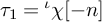 $\tau _1 = {}^\iota \chi [-n] $
or
 $ {}^\iota \chi ^{-1}[n].$
This proves that
 $I_b^S(\chi _f, \sigma _f)_w \oplus I_b^S(\chi _f^{-1}[2n], \sigma _f)_{w'}$
is isotypic in
 $H^{\mathfrak {q}_b} (\partial {\mathcal S}^G_{K_{f}}, {\mathcal M}_{\lambda ,E})$
. Furthermore, recalling that in the definition of the modules
 $I_b^S(\chi _f, \sigma _f)_w$
and
 $I_b^S(\chi _f^{-1}[2n], \sigma _f)_{w'}$
we first take the isotypic components of
 $\chi _f \times \sigma _f$
and
 $\chi _f^{-1}[2n] \times {}^{\kappa _{2n}}\sigma _f$
and then induce, the same argument as above proves (77).
8 Rank-one Eisenstein cohomology
An indispensable tool for our main theorem on Eisenstein cohomology is Poincaré duality which gives that the image of total cohomology in the cohomology of the boundary is in fact a maximal isotropic subspace. We briefly review Poincaré duality in our context and refer the reader to [Reference Harder and Raghuram16, Sect. 6.1] for more details.
8.1 Poincaré duality
The maps in the long exact sequence in cohomology from 1.6.2 relate Poincaré duality for
 ${\mathcal S}^G_{K_{f}}$
and
 $\partial {\mathcal S}^G_{K_{f}}$
as in the following diagram:

where
 $\textsf {d} := \mathrm {dim}( {\mathcal S}^G_{K_{f}})$
and
 $ \textsf {d}-1= \mathrm {dim}( \partial {\mathcal S}^G_{K_{f}})$
, and the duality maps are the horizontal arrows. Define Eisenstein cohomology as
 $$ \begin{align*}H^q_{\mathrm{Eis}}(\partial {\mathcal S}^G_{K_{f}},\widetilde {\mathcal M}_{\lambda,E}) \ := \ \text{Image}\left(H^{q} ( {\mathcal S}^G_{K_{f}}, \widetilde{\mathcal M}_{\lambda,E})\xrightarrow{\mathfrak r^{\bullet}} H^q (\partial {\mathcal S}^G_{K_{f}}, \widetilde{\mathcal M}_{\lambda,E})\right). \end{align*} $$
It follows from the above diagram as in [Reference Harder and Raghuram16, Prop. 6.1] that
 $H^q_{\mathrm {Eis}}(\partial {\mathcal S}^G_{K_{f}}, {\mathcal M}_{\lambda ,E})$
is a maximal isotropic subspace of boundary cohomology; that is,
 $$ \begin{align} H^q_{\mathrm{Eis}}(\partial {\mathcal S}^G_{K_{f}},\widetilde {\mathcal M}_{\lambda,E}) = H^{\mathsf{d} - 1 -q}_{\mathrm{Eis}}((\partial {\mathcal S}^G_{K_{f}}, \widetilde{\mathcal M}_{\lambda^{\mathsf{v}},E})^{\perp}. \end{align} $$
8.2 The main theorem on rank-one Eisenstein cohomology
The following theorem is the generalization of Theorem 6.2 of [Reference Harder and Raghuram16] to our context of orthogonal groups:
Theorem 80. Define the images of Eisenstein cohomology under the Hecke-equivariant maps
 ${\mathcal R}$
of Theorem69 as
 $$ \begin{align*}\mathfrak{I}_b^S(\chi_f, \sigma_f) \ := \ {\mathcal R}^{b}_{\chi_f, \sigma_f}(H^{\mathfrak{q}_b}_{\mathrm{Eis}}(\partial {\mathcal S}^G, \widetilde{\mathcal{M}}_{\lambda,E})^{K_f}), \end{align*} $$
 $$ \begin{align*}\mathfrak{I}_t^S(\chi_f, \sigma_f) \ := \ {\mathcal R}^{t}_{\chi_f, \sigma_f}(H^{\mathfrak{q}_t}_{\mathrm{Eis}}(\partial {\mathcal S}^G, \widetilde{\mathcal{M}}_{\lambda^{\mathsf{v}},E})^{K_f}). \end{align*} $$
We have the following:
-
(i)
$\mathfrak {I}_b^S(\chi _f, \sigma _f)$
is a
$\mathsf {k}$
-dimensional subspace of
$$ \begin{align*}I_b^S(\chi_f, \sigma_f)_w \ \oplus \ I_b^S(\chi_f^{-1}[2n], \sigma_f)_{w'}. \end{align*} $$
-
(ii)
$\mathfrak {I}_t^S(\chi _f, \sigma _f)$
is a
$\mathsf {k}$
-dimensional subspace of
$$ \begin{align*}I_t^S(\chi_f^{-1}[2n], \sigma_f)_{w^{\mathsf{v}}} \ \oplus \ I_t^S(\chi_f, \sigma_f)_{w^{\mathsf{v}}{}'}. \end{align*} $$


Proof. The proof is very similar to the proof of Theorem 6.2 of [Reference Harder and Raghuram16] with some fine differences; we adumbrate the proof while explaining such differences and refer the reader to loc.cit. for more details. There are two steps. The first step (as in [Reference Harder and Raghuram16, 6.2.2.1]) is to show that these images are at least
 $\mathsf {k}$
-dimensional; this is achieved after a base-change via an
 $\iota \in \mathrm {Hom}(E,{\mathbb C})$
and showing the resulting spaces are at least
 $\mathsf {k}$
-dimensional. Suppose
 $(d, \mu )$
is on the right of unitary axis. To begin, we describe the base-change to
 ${\mathbb C}$
via
 $\iota $
of
 $I_b^S(\chi _f, \sigma _f)_w$
; similar descriptions apply to the other induced modules in (i) and (ii). Tensoring (68) by
 ${\mathbb C}$
via
 $\iota $
, using (30) for the inducing data, and Proposition 56, we get
 $$ \begin{align} I_b^S(\chi_f, \sigma_f)_w \otimes_{E, \iota} {\mathbb C} \ \cong \ \bigoplus_{j=1}^l H^{\mathfrak{q}_b}\left({\mathfrak g}({\mathbb R}), \overline{K}_\infty; \ {}^{\mathrm{a}}\mathrm{Ind}_{P({\mathbb A})}^{G({\mathbb A})}({}^\iota\chi \otimes V_{{}^\iota\sigma_j})^{K_f} \otimes {\mathcal M}_{{}^\iota\lambda}\right), \end{align} $$
where the j-th summand, using the inverse of
 $\Phi _j$
in the inducing data, is equivalent to
 $$ \begin{align*}H^{\mathfrak{q}_b}\left({\mathfrak g}({\mathbb R}), \overline{K}_\infty; \ {}^{\mathrm{a}}\mathrm{Ind}_{P({\mathbb R})}^{G({\mathbb R})}({}^\iota\chi_\infty \otimes {}^\iota\sigma_{j, \infty}) \otimes {\mathcal M}_{{}^\iota\lambda}\right) \otimes {}^{\mathrm{a}}\mathrm{Ind}_{P({\mathbb A}_f)}^{G({\mathbb A}_f)}({}^\iota\chi_f \otimes {}^\iota\sigma_{j,f})^{K_f}, \end{align*} $$
with the relative Lie algebra cohomology group being one-dimensional. Similarly, we have
 $$ \begin{align*}I_b^S(\chi_f^{-1}[2n], \sigma_f)_w \otimes_{E, \iota} {\mathbb C} \ \cong \ \bigoplus_{j=1}^l H^{\mathfrak{q}_b}\left({\mathfrak g}({\mathbb R}), \overline{K}_\infty; \ {}^{\mathrm{a}}\mathrm{Ind}_{P({\mathbb A})}^{G({\mathbb A})}({}^\iota\chi^{-1}[2n] \otimes V_{{}^{\kappa_{2n}\iota}\sigma_j})^{K_f} \otimes {\mathcal M}_{{}^\iota\lambda}\right). \end{align*} $$
For each j, for brevity, we let
 $T_{\mathrm {st},j}^\bullet $
denote the map induced by applying the functor
 $H^{\mathfrak {q}_b}\left({\mathfrak g}({\mathbb R}), \overline {K}_\infty; \, - \otimes {\mathcal M}_{{}^\iota \lambda } \right)$
to the standard intertwining operator
 $T_{\mathrm {st}}(-n, w_{P}, {}^\iota \chi \times {}^\iota \sigma _j)$
:
 $$ \begin{align*}H^{\mathfrak{q}_b}\left({\mathfrak g}({\mathbb R}), \overline{K}_\infty; \, - \otimes {\mathcal M}_{{}^\iota\lambda} \right)(T_{\mathrm{st}}(-n, w_{P}, {}^\iota\chi \times {}^\iota\sigma_j)). \end{align*} $$
Using Theorem 43 and Section 3.3, we see that
 $\mathfrak {I}_b^S(\chi _f, \sigma _f) \otimes _{E,\iota } {\mathbb C}$
at least contains all cohomology classes of the form
 $$ \begin{align} \left\{ \left(f_1, \ldots, f_l \right), \ \left((f_1 + T_{\mathrm{st},1}^\bullet(f_1)), \ldots, (f_l + T_{\mathrm{st},l}^\bullet(f_l))\right) \right\}, \end{align} $$
where
-
(1)
$f_j \in H^{\mathfrak {q}_b}\left({\mathfrak g}({\mathbb R}), \overline {K}_\infty; \ {}^{\mathrm {a}}\mathrm {Ind}_{P({\mathbb A})}^{G({\mathbb A})}({}^\iota \chi \otimes V_{{}^\iota \sigma _j})^{K_f} \otimes {\mathcal M}_{{}^\iota \lambda }\right);$
-
(2)
$(f_1, \ldots , f_l) \in I_b^S(\chi _f, \sigma _f)_w \otimes _{E,\iota } {\mathbb C} ;$
and -
(3)
$\left( (f_1 + T_{\mathrm {st},1}^\bullet (f_1)), \ldots , (f_l + T_{\mathrm {st},l}^\bullet (f_l)) \, \right) \in I_b^S(\chi _f^{-1}[2n], \sigma _f)_{w'} \otimes _{E,\iota } {\mathbb C}.$


Hence,
 $\dim _E(\mathfrak {I}_b^S(\chi _f, \sigma _f)) = \dim _{\mathbb C}(\mathfrak {I}_b^S(\chi _f, \sigma _f) \otimes _{E,\iota } {\mathbb C}) \geq \dim _{\mathbb C}(I_b^S(\chi _f, \sigma _f)_w \otimes _{E,\iota }{\mathbb C}) = \mathsf {k}.$
If
 $(d, \mu )$
is on the left of unitary axis, then
 $(-d-2n, {}^{\kappa _{2n}} \mu )$
is on the right of unitary axis, and hence, by working with the intertwining maps
 $T_{\mathrm {st}}(n, w_{P_0}, {}^\iota \chi ^{-1}[-2n] \times {}^{\kappa _{2n} \iota }\sigma _j)$
, we get the desired result. Similarly, we also get
 $\mathfrak {I}_t^S(\chi _f, \sigma _f)$
is at least
 $\mathsf {k}$
-dimensional. (In [Reference Harder and Raghuram16], by strong multiplicity-one for general linear groups, we have
 $l = 1$
; however, for orthogonal groups, in general,
 $l> 1$
, and this necessitates extra care in the final proof in Section 9.2.)
The second step (as in [Reference Harder and Raghuram16, 6.2.2.2]) involves the Poincaré duality pairing (78) to show that both are exactly
 $\textsf {k}$
-dimensional E-vector spaces; one of the fine differences alluded to concerns the setting up of the relevant exercise in linear algebra to make this conclusion, which we now discuss. For brevity, let
 ${\mathcal V} = I_b^S(\chi _f, \sigma _f)_w \ \oplus \ I_b^S(\chi _f^{-1}[2n], \sigma _f)_{w'}$
and
 ${\mathcal W} = I_t^S(\chi _f^{-1}[2n], \sigma _f)_{w^{\mathsf {v}}} \ \oplus \ I_t^S(\chi _f, \sigma _f)_{w^{\mathsf {v}}{}'}.$
Since,
 ${\mathcal V} \subset H^{\mathfrak {q}_b}(\partial {\mathcal S}^G, \widetilde {\mathcal {M}}_{\lambda ,E})^{K_f}$
and
 ${\mathcal W} \subset H^{\mathfrak {q}_t}(\partial {\mathcal S}^G, \widetilde {\mathcal {M}}_{\lambda ^{\mathsf {v}},E})^{K_f}$
, the Poincaré duality pairing in the bottom horizontal arrow in (78) restricts to a pairing on
 $(\ , \ ) : {\mathcal V} \times {\mathcal W} \to E.$
This pairing need not be perfect in general, but in our situation, the induced map
 ${\mathcal V} \to {\mathcal W}^*$
is injective. This is because in the bottom-degree we have all possible occurrences of
 $\chi _f \times \sigma _f$
accounted for, which is reflected by
 $\wedge ^0{\mathfrak a}^*$
being one-dimensional. In contrast, in the top-degree, we would have
 $\wedge ^{\mathsf {r}_F-1}{\mathfrak a}^*,$
which is
 $\mathsf {r}_F$
-dimensional that is greater than one if
 $F \neq {\mathbb Q}$
; see Remark 60. Now, for brevity, let
 $\mathfrak {I}_b = \mathfrak {I}_b^S(\chi _f, \sigma _f) \subset {\mathcal V}$
and
 $\mathfrak {I}_t := \mathfrak {I}_t^S(\chi _f, \sigma _f) \subset {\mathcal W}.$
From (79), we have
 $(\mathfrak {I}_b, \mathfrak {I}_t) = 0.$
The injective map
 ${\mathcal V} \to {\mathcal W}^*$
induces an injection
 $\mathfrak {I}_b \to ({\mathcal W}/\mathfrak {I}_t)^*$
. Together with the conclusion of the first step, we get
 $$ \begin{align*}\mathsf{k} \ \leq \ \dim(\mathfrak{I}_b) \ \leq \ \dim({\mathcal W}/\mathfrak{I}_t)^* \ \leq \ \mathsf{k}, \end{align*} $$
giving us
 $\mathsf {k} = \dim (\mathfrak {I}_b) = \dim (\mathfrak {I}_t).$
The above theorem is best appreciated by pretending
 $\mathsf {k} = 1$
, in which case, it says that the image of total Eisenstein cohomology, via the rank-one Eisenstein cohomology for P, inside a
 $2$
-dimensional isotypic subspace is one-dimensional (i.e., a line in a
 $2$
-dimensional vector space over E). The slope of this line is an element of E, which after passing to a transcendental situation is related to a ratio of L-values, hence giving us a rationality result for that ratio; this is the essence of the proof of our main theorem on special values of L-functions.
The embedding
 $\Phi _j$
in (29) of the cuspidal representation
 ${}^\iota \sigma _j$
into the space of cusp forms on
 ${}^\circ M$
, which we recall is unique up to a nonzero complex number, is used in the above proof. However, since the same
 $\Phi _j$
shows up on either side of the intertwining operator
 $$ \begin{align*}T_{\mathrm{st}}(-n, w_{P}, {}^\iota\chi \times {}^\iota\sigma_j) : {}^{\mathrm{a}}\mathrm{Ind}_{P({\mathbb A})}^{G({\mathbb A})}\left({}^\iota\chi \otimes \Phi_j({}^\iota\sigma_j)\right) \ \longrightarrow \ {}^{\mathrm{a}}\mathrm{Ind}_{P({\mathbb A})}^{G({\mathbb A})}\left({}^\iota\chi^{-1}[2n] \otimes \Phi_j({}^{\kappa_{2n}\iota}\sigma_j)\right), \end{align*} $$
we deduce that the map
 $T_{\mathrm {st},j}^\bullet $
independent of the choice of
 $\Phi _j.$
9 Proof of the main theorem on L-values
We are now in a position to give a proof of Theorem 1.
9.1 ‘Right Vs Left’ of the unitary axis
As in Section 6, just for this subsection, the
 $\iota : E \to {\mathbb C}$
is fixed and so, for brevity, we suppress it from notation. In Section 9.2, we will show, under the condition
 $1 - \mu _{\mathrm {min}} \leq -(d+n) \leq \mu _{\mathrm {min}} -1$
for
 $(d,\mu )$
, an algebraicity result for the ratio
 $$ \begin{align*}\frac{L(-n, \, \chi \times \sigma)}{L(1-n, \, \chi \times \sigma)} \ = \ \frac{L(-n-d, \, \chi^\circ \times \sigma)}{L(1-n-d, \, \chi^\circ \times \sigma)} \end{align*} $$
when
 $(d, \mu )$
is on the right of the unitary axis (i.e., when
 $-(d+n) \geq 0$
). The above restrictions on
 $-(d+n)$
together gives
 $0 \leq -(n+d) \leq \mu _{\mathrm {min}} - 1.$
Letting d vary within these bounds, we get an algebraicity theorem for the ratios:
 $$ \begin{align} \left\{ \frac{L(0, \, \chi^\circ \times \sigma)}{L(1, \, \chi^{\circ} \times \sigma)}, \ \ \frac{L(1, \, \chi^\circ \times \sigma)}{L(2, \, \chi^{\circ} \times \sigma)}, \ \ \dots \ , \ \ \frac{L(\mu_{\mathrm{min}}-1, \, \chi^\circ \times \sigma)}{L(\mu_{\mathrm{min}}, \, \chi^{\circ} \times \sigma)} \right\}. \end{align} $$
The critical set
 $\{ 1- \mu _{\mathrm {min}}, \, 2- \mu _{\mathrm {min}}, \dots , \mu _{\mathrm {min}}\}$
for
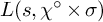 $L(s,\, \chi ^{\circ } \times \sigma )$
contains
 $2\mu _{\mathrm {min}}-1$
pairs of successive integers, and (83) covers only
 $\mu _{\mathrm {min}}$
successive pairs. For the remaining
 $\mu _{\mathrm {min}}-1$
ratios of successive L-values,
 $$ \begin{align} \left\{\frac{L(1-\mu_{\mathrm{min}}, \, \chi^\circ \times \sigma)}{L(2-\mu_{\mathrm{min}}, \, \chi^{\circ} \times \sigma)}, \ \ \dots \ , \ \ \frac{L(-1, \, \chi^\circ \times \sigma)}{L(0, \, \chi^{\circ} \times \sigma)} \right\}, \end{align} $$
we can start from the other side of the intertwining operator:
 $$ \begin{align*}T_{\mathrm{st}}(s)|_{s = -n} \ : \ {}^{\mathrm{a}}\mathrm{Ind}_{P({\mathbb A})}^{G({\mathbb A})} \left(\chi \times \sigma \right) \ \longrightarrow \ {}^{\mathrm{a}}\mathrm{Ind}_{P({\mathbb A})}^{G({\mathbb A})} \left(\chi^{-1}[2n] \times {}^{\kappa_{2n}}\sigma \right); \end{align*} $$
that is, we consider the standard intertwining operator
 $$ \begin{align*}T_{\mathrm{st}}(s, w_{P_0}, \chi^{-1} \times {}^{\kappa_{2n}} \sigma) \ : \ I(s, \chi^{-1} \times {}^{\kappa_{2n}} \sigma ) \ \longrightarrow \ I(-s, \chi \times \sigma) \end{align*} $$
at its point of evaluation which is
 $s = n$
. If
 $(d,\mu )$
corresponds to
 $(\chi , \sigma )$
, then
 $(-d-2n, {}^{\kappa _{2n}}\mu )$
corresponds to
 $(\chi ^{-1}[2n] , {}^{\kappa _{2n}}\sigma ).$
Since, locally,
 ${}^{\kappa _{2n}}(\mu _1, \dots , \mu _{n-1}, \mu _n) = (\mu _1, \dots , \mu _{n-1}, -\mu _n),$
we deduce that
 $\mu _{\mathrm {min}} = ({}^{\kappa _{2n}}\mu )_{\mathrm {min}}.$
The condition
 $1 - \mu _{\mathrm {min}} \leq -(d+n) \leq \mu _{\mathrm {min}} -1$
imposed by the combinatorial lemma for
 $(d,\mu )$
is identical to the those on
 $(-d-2n, {}^{\kappa _{2n}}\mu ).$
Next, if
 $(d,\mu )$
is on the left of the unitary axis (i.e., if
 $-(d+n) < 0$
which is
 $(d+n) \geq 1$
), then for
 $(-d-2n, {}^{\kappa _{2n}}\mu )$
, we have
 $-(-d-2n)-n \geq 1$
, or that
 $(-d-2n, {}^{\kappa _{2n}}\mu )$
is strictly to the right of its unitary axis, giving us an algebraicity theorem for
 $$ \begin{align*}\frac{L(n, \, \chi^{-1} \times {}^{\kappa_{2n}} \sigma )}{L(1+n, \, \chi^{-1} \times {}^{\kappa_{2n}} \sigma )} \ = \ \frac{L(n+d, \, \chi^\circ{}^{-1} \times {}^{\kappa_{2n}} \sigma )}{L(1+n+d, \, \chi^\circ{}^{-1} \times {}^{\kappa_{2n}} \sigma )}. \end{align*} $$
So when
 $(d, \mu )$
is on the left of the unitary axis, together with the combinatorial lemma, the restrictions are
 $1 \ \leq \ d+n \ \leq \ \mu _{\mathrm {min}}-1$
; and if we let d vary within this range, we get an algebraicity theorem for the ratios of L-values:
 $$ \begin{align} \left\{ \frac{L(1, \, \chi^\circ{}^{-1} \times {}^{\kappa_{2n}} \sigma )}{L(2, \, \chi^\circ{}^{-1} \times {}^{\kappa_{2n}} \sigma )}, \ \ \dots \ , \ \ \frac{L(\mu_{\mathrm{min}}-1, \, \chi^\circ{}^{-1} \times {}^{\kappa_{2n}} \sigma )}{L(\mu_{\mathrm{min}}, \, \chi^\circ{}^{-1} \times {}^{\kappa_{2n}} \sigma )} \right\}. \end{align} $$
To compare the lists in (84) and (85), we use the global functional equation
 $$ \begin{align*}L(s, \, \chi^\circ \times \sigma) \ = \ \varepsilon(s, \, \chi^\circ \times \sigma) L(1-s, \, \chi^\circ{}^{-1} \times \sigma^{\mathsf{v}}), \end{align*} $$
together with the easy observations (i)
 ${}^{\kappa _{2n}} \sigma = \sigma $
since
 $\kappa _{2n} \in \mathrm {O}(2n)$
, and (ii)
 $\sigma ^{\mathsf {v}} = \sigma $
since both are nearly equivalent (as easy observation on their Satake parameters), having the same cuspidal Arthur parameter and being globally generic with respect to the same Whittaker datum. The global
 $\varepsilon $
-factor is a product of local
 $\varepsilon $
-factors. At a non-archimedean place v, the local
 $\varepsilon $
-factor is of the form
 $W(\chi _v \times \sigma _v)\, q_v^{(1/2 -s)(c_v)}$
where
 $W(\chi _v \times \sigma _v)$
is the local root number and
 $c_v$
is the sum of conductoral exponents of the data. Thus, the ratio of local
 $\varepsilon $
-factors at two successive integers is a nonzero rational number. At an archimedean place, the local
 $\varepsilon $
-factor is a constant. Hence, the ratio of global
 $\varepsilon $
-factors at two successive integers is a nonzero rational number. Finally, we note all the individual L-values in (84) and (85) are nonvanishing, since
 $L(s, \chi ^\circ \times \Psi (\sigma )) \neq 0$
for any integer value of s, by the unitarity of
 $\Psi (\sigma )$
and
 $\chi ^\circ $
, and appealing to the theorem of Jacquet–Shalika [Reference Jacquet and Shalika19]. We get the equalities
 $$ \begin{align*} \frac{L(1, \, \chi^\circ{}^{-1} \times {}^{\kappa_{2n}} \sigma )}{L(2, \, \chi^\circ{}^{-1} \times {}^{\kappa_{2n}} \sigma )} \ \approx_{{\mathbb Q}^\times} \ &\frac{L(0, \, \chi^\circ \times \sigma)}{L(-1, \, \chi^{\circ} \times \sigma)}, \ \ \dots \ \ , \\ &\qquad \frac{L(\mu_{\mathrm{min}}-1, \, \chi^\circ{}^{-1} \times {}^{\kappa_{2n}} \sigma )}{L(\mu_{\mathrm{min}}, \, \chi^\circ{}^{-1} \times {}^{\kappa_{2n}} \sigma )} \ \approx_{{\mathbb Q}^\times} \ \frac{L(2-\mu_{\mathrm{min}}, \, \chi^\circ \times \sigma)}{L(1-\mu_{\mathrm{min}}, \, \chi^{\circ} \times \sigma)}, \end{align*} $$
which show that an algebraicity result for the ratios of L-values in (85) implies an algebraicity result for the (reciprocals of the) ratios of L-values in (84).
9.2 Conclusion of proof
We need to prove that when
 $(d, \mu )$
is on the right of the unitary axis and also satisfies the condition imposed by the combinatorial lemma (i.e, when
 $0 \leq -(d+n) \leq \mu _{\mathrm {min}} -1),$
then
 $L(-n, \, {}^\iota \chi \times {}^\iota \sigma )/L(1-n, \ {}^\iota \chi \times {}^\iota \sigma ) \in \iota (E),$
and that for all
 $\eta \in \mathrm {Gal}(\bar {{\mathbb Q}}/ {\mathbb Q})$
, we have the reciprocity law as in
 $(iii)$
of Theorem 1.
From Theorem 80, we have
 $\mathfrak {I}_b^S(\chi _f, \sigma _f)$
is a
 $\mathsf {k}$
-dimensional subspace inside the
 $2 \mathsf {k}$
-dimensional space
 $I_b^S(\chi _f, \sigma _f)_w \ \oplus \ I_b^S(\chi _f^{-1}[2n], \sigma _f)_{w'}.$
From the proof of Theorem 80, it follows that we have an E-linear map
 $T_{\mathrm {Eis}} := T_{\mathrm {Eis}}(\chi _f, \sigma _f) : I_b^S(\chi _f, \sigma _f)_w \ \to \ I_b^S(\chi _f^{-1}[2n], \sigma _f)_{w'},$
such that
 $$ \begin{align} \mathfrak{I}_b^S(\chi_f, \sigma_f) \ = \ \left\{ (\xi, \, \xi + T_{\mathrm{Eis}}(\xi) \ | \ \xi \in I_b^S(\chi_f, \sigma_f)_w \right\}. \end{align} $$
Take
 $\iota : E \rightarrow {\mathbb C},$
and base change to
 ${\mathbb C}$
via
 $\iota $
to consider the map
 $T_{\mathrm {Eis}} \otimes _{E,\iota } 1_{\mathbb C}$
.
The domain and codomain of
 $T_{\mathrm {Eis}} \otimes _{E,\iota } 1_{\mathbb C}$
have l many summands (for the domain, see (81), with a similar description for the codomain), and it seems like we have a period matrix, but from the proof of Theorem 80 (see especially (82)), it follows that
 $T_{\mathrm {Eis}} \otimes _{E,\iota } 1_{\mathbb C}$
is the ‘diagonal matrix’
 $(\mathbf {1}_j + T_{\mathrm {st},j}^\bullet )_{j=1}^{l};$
the notation for the j-th term being clear from context. We contend that this diagonal matrix, up to the ratio of critical values
 $L(-n, {}^\iota \chi \times {}^\iota \sigma )/L(1-n, {}^\iota \chi \times {}^\iota \sigma )$
is
 $\iota (E)$
-rational; this is the essence of the rest of the proof.
For
 $v \in S_{\infty }$
, and
 $1 \leq j \leq l$
, the local representation
 $^{\iota } \sigma _{j,v}$
is a discrete series representation in the same L-packet of
 ${\mathbb D}_{\mu ^{v}}^\dagger $
; hence, for all
 $1 \leq j \leq l$
, we get an equality of the archimedean L-factors
 $L(s, {}^\iota \chi _v \times {}^\iota \sigma _{j,v}) = L(s, {}^\iota \chi _v \times {}^\iota \sigma _{v}).$
Whence, from Proposition 62, for each
 $1 \leq j \leq l,$
we have the relative Lie algebra cohomology classes at infinity,
 $[\mathscr {I}^0_j]$
and
 $[\tilde {\mathscr {I}}^0_j],$
and that
 $$ \begin{align*}T_{\mathrm{st}, j, \infty}^{\bullet} ([\mathscr{I}^0_j] ) \ \approx_{{\mathbb Q}^\times} \ \frac{L_\infty(-n, {}^\iota\chi \times {}^\iota\sigma_{j}) }{L_\infty(1-n, {}^\iota\chi \times {}^\iota\sigma_{j})} [\tilde{\mathscr{I}}^0_j] \ = \ \frac{L_\infty(-n, {}^\iota\chi \times {}^\iota\sigma) }{L_\infty(1-n, {}^\iota\chi \times {}^\iota\sigma)} [\tilde{\mathscr{I}}^0_j]. \end{align*} $$
Let us define a map
 $$ \begin{align*} T_{\mathrm{loc}, j, \infty}^{\bullet} : H^{\mathfrak{q}_b}\left({\mathfrak g}({\mathbb R}), \overline{K}_\infty; \, {}^{\mathrm{a}}\mathrm{Ind}_{P({\mathbb R})}^{G({\mathbb R})}({}^\iota\chi_\infty \otimes {}^\iota\sigma_{j, \infty}) \otimes {\mathcal M}_{{}^\iota\!\lambda,{\mathbb C}}\right) \ &\to \\ &\hspace{-120pt} H^{\mathfrak{q}_b}\left({\mathfrak g}({\mathbb R}), \overline{K}_\infty; \, {}^{\mathrm{a}}\mathrm{Ind}_{P({\mathbb R})}^{G({\mathbb R})}({}^\iota\chi_\infty^{-1}[2n] \otimes {}^\iota{}^{\kappa_{2n}}\sigma_{j, \infty}) \otimes {\mathcal M}_{{}^\iota\!\lambda,{\mathbb C}}\right), \end{align*} $$
which is characterised by
 $T_{\mathrm {loc}, j, \infty }^{\bullet } ([\mathscr {I}^0_j]) \ \approx _{{\mathbb Q}^\times } \ [\tilde {\mathscr {I}}^0_j]$
and such that
 $$ \begin{align} T_{\mathrm{st}, j, \infty}^{\bullet} \ = \ \frac{L_\infty(-n, {}^\iota\chi \times {}^\iota\sigma) }{L_\infty(1-n, {}^\iota\chi \times {}^\iota\sigma)} T_{\mathrm{loc}, j, \infty}^{\bullet}. \end{align} $$
For
 $v \notin S_\infty $
, we have
 ${}^\iota \sigma _{j,v} = {}^\iota \sigma _v.$
In particular, the discussion for the standard intertwining operator for the j-th summand is independent of j, and we suppress the subscript j for what follows at finite places.
For
 $v \notin S$
(recall that S includes
 $S_\infty $
and all finite ramified places), if
 $f_v^0$
and
 $\tilde {f_v^0}$
are the normalised spherical vectors, respectively, then from (42) at our point of evaluation
 $s = -n$
, we get
 $$ \begin{align*}T_{\mathrm{st},v} (f_v^\circ) = \dfrac{L(-n, ~\!\!^\iota \chi_v \times~\!\! ^\iota\sigma_{v})}{L(1-n, ~\!\!^\iota \chi_v \times~\!\! ^\iota\sigma_{v})} \tilde{f}_v^\circ. \end{align*} $$
For
 $v \notin S$
, define
 $$ \begin{align*}T_{\mathrm{loc},v} : = \left( \dfrac{L(-n, {}^\iota \chi_v \times {}^\iota\sigma_v)}{L(1-n, {}^\iota \chi_v \times {}^\iota\sigma_v)} \right)^{-1} T_{\mathrm{st},v}, \end{align*} $$
which is characterised by
 $T_{\mathrm {loc},v}(f_v^\circ ) = \tilde {f}_v^\circ .$
It is clear then that
 $T_{\mathrm {loc},v}$
is the base change via
 $\iota $
of a map defined over E (i.e., there exists an E-linear map
 $T_{\mathrm { loc},v,0} $
such that
 $T_{\mathrm {loc},v} = T_{\mathrm {loc},v,0} \otimes _{E, \iota } 1_{{\mathbb C}}).$
Now define
 $T^S_{\mathrm {loc}} = \otimes _{v \notin S} T_{\mathrm {loc},v}$
and
 $T^S_{\mathrm {loc},0} = \otimes _{v \notin S} T_{\mathrm {loc},v,0};$
we have
 $$ \begin{align*}T^S_{\mathrm{loc}} = T^S_{\mathrm{loc},0} \otimes_{E, \iota} 1_{{\mathbb C}}. \end{align*} $$
Putting together the discussion for
 $v \notin S$
, we have
 $$ \begin{align} T_{\mathrm{st}}^S \ := \ \bigotimes_{v \notin S} T_{\mathrm{st},v} \ = \ \dfrac{L^{S}(-n, {}^\iota \chi \times {}^\iota\sigma)}{L^{S}(1-n, {}^\iota \chi \times {}^\iota\sigma)} \left(T^S_{\mathrm{loc},0} \otimes_{E, \iota} 1_{{\mathbb C}} \right), \end{align} $$
where
 $L^{S}(s, {}^\iota \chi \times {}^\iota \sigma ) = \prod _{v \notin S} L^{S}(s, {}^\iota \chi _v \times {}^\iota \sigma _v)$
is the partial L-function.
For
 $v \in S \setminus S_\infty $
, the normalised intertwining operator in (63) and its arithmetic version in (66) can be put together, while invoking the hypothesis in (65), to give (for any
 $1 \leq j \leq l$
),
 $$ \begin{align} T_{\mathrm{st}, v}(-n) \ = \ \left( \dfrac{L(-n, {}^\iota \chi_v \times {}^\iota\sigma_v)}{L(1-n, {}^\iota \chi_v \times {}^\iota\sigma_v)} \right) \, T_{\mathrm{arith}, v} \otimes_{E, \iota} 1_{\mathbb C}. \end{align} $$
Putting these calculations together, while partitioning the set of all places as the disjoint union
 $S_\infty \cup (S\setminus S_\infty ) \cup \{v : v \notin S\}$
, we have
 $$ \begin{align} T_{\mathrm{Eis}}(\chi_f, \sigma_f) \otimes_{E,\iota} 1_{{\mathbb C}} \ = \ \left(\mathbf{1}_j, \ (T_{\mathrm{st}, j, \infty}^{\bullet} \ \otimes \ (\otimes_{v \in S \setminus S_{\infty}} T_{\mathrm{st},v}) \ \otimes \ (T_{\mathrm{st}}^S) \right)_{1 \leq j \leq l}. \end{align} $$
Let
 $T_{\mathrm {Eis}}^1(\chi _f, \sigma _f) := T_{\mathrm {Eis}}(\chi _f, \sigma _f) - \mathbf {1}$
. Using (87), (88), (89), and (90), we get
 $$ \begin{align} &T_{\mathrm{Eis}}^1(\chi_f, \sigma_f) \otimes_{E,\iota} 1_{{\mathbb C}} \nonumber\\ &\quad =\dfrac{L(-n, {}^\iota \chi \times {}^\iota\sigma)}{L(1-n, {}^\iota \chi \times {}^\iota\sigma)} \ \left(\left( T_{\mathrm{loc}, j, \infty}^{\bullet} \otimes_E T^S_{\mathrm{loc},0} \otimes_E (\otimes_{v \in S\setminus S_\infty} T_{\mathrm{arith}, v}) \right) \otimes_{E, \iota} 1_{\mathbb C} \right)_{1 \leq j \leq l}. \end{align} $$
It follows that
 $$ \begin{align*}\dfrac{L(-n, {}^\iota \chi \times {}^\iota\sigma)}{L(1-n, {}^\iota \chi \times {}^\iota\sigma)} \in \iota(E). \end{align*} $$
For Galois equivariance in
 $(iii)$
of Theorem 1, consider the action of
 $\eta \in \mathrm {Gal}(\bar {{\mathbb Q}} / {\mathbb Q})$
on
 $\iota \in \mathrm {Hom}(E, \bar {{\mathbb Q}}) = \mathrm {Hom}(E, {\mathbb C})$
by
 $\eta _{\ast }(\iota ) = \eta \circ \iota $
. We hit the diagram in (76) by
 $\eta $
, and by functoriality of the cohomology groups as in [Reference Harder and Raghuram16, 2.3.3], we get
 $$ \begin{align*}\eta^{\bullet}(T_{\mathrm{Eis}}^1(\chi_f, \sigma_f)) \ = \ T_{\mathrm{Eis}}^1({}^\eta\chi_f, {}^\eta\sigma_f). \end{align*} $$
For brevity, let’s put
 $T_{\mathrm {loc}}(\chi _f, \sigma _f) = \left( T_{\mathrm {loc}, j, \infty }^{\bullet } \otimes _E T^S_{\mathrm {loc},0} \otimes _E (\otimes _{v \in S\setminus S_\infty } T_{\mathrm {arith}, v}) \right)_j$
for what shows up in the right-hand side of (91), and also put
 $$ \begin{align*}\mathscr{L}({}^\iota \chi \times {}^\iota\sigma) \ = \ L(-n, {}^\iota \chi \times {}^\iota\sigma)/L(1-n, {}^\iota \chi \times {}^\iota\sigma). \end{align*} $$
Then, we may rewrite (91), while using
 $\iota $
to base-change to
 $\bar {{\mathbb Q}}$
, as
 $$ \begin{align*}T_{\mathrm{Eis}}^1(\chi_f, \sigma_f) \otimes_{E,\iota} 1_{\bar{{\mathbb Q}}} \ = \ T_{\mathrm{loc}}(\chi_f, \sigma_f) \otimes_{E,\iota} \mathscr{L}({}^\iota \chi \times {}^\iota\sigma) 1_{\bar{{\mathbb Q}}}. \end{align*} $$
On the one hand, we have
 $$ \begin{align*} &(1\otimes \eta) \circ (T_{\mathrm{Eis}}^1(\chi_f, \sigma_f) \otimes_{E,\iota} 1_{\bar{{\mathbb Q}}}) \ = \ \eta^{\bullet}(T_{\mathrm{Eis}}^1(\chi_f, \sigma_f)) \otimes_{E, \eta \circ \iota} \eta \ = \\ &T_{\mathrm{Eis}}^1({}^\eta\chi_f, {}^\eta\sigma_f) \otimes_{E, \eta \circ \iota} \eta \ = \ T_{\mathrm{loc}}({}^\eta\chi_f, {}^\eta\sigma_f) \otimes_{E, \eta \circ \iota} \mathscr{L}({}^{\eta\circ\iota} \chi \times {}^{\eta\circ\iota}\sigma) \eta, \end{align*} $$
and on the other hand, we have
 $$ \begin{align*} &(1\otimes \eta) \circ (T_{\mathrm{Eis}}^1(\chi_f, \sigma_f) \otimes_{E,\iota} 1_{\bar{{\mathbb Q}}}) \ = \ (1\otimes \eta) \circ (T_{\mathrm{loc}}(\chi_f, \sigma_f) \otimes_{E,\iota} \mathscr{L}({}^\iota \chi \times {}^\iota\sigma) 1_{\bar{{\mathbb Q}}}) \ = \\ &\eta^\bullet T_{\mathrm{loc}}(\chi_f, \sigma_f) \otimes_{E, \eta \circ \iota} \eta(\mathscr{L}({}^\iota \chi \times {}^\iota\sigma)) \eta \ = \ T_{\mathrm{loc}}({}^\eta\chi_f, {}^\eta\sigma_f) \otimes_{E, \eta \circ \iota} \eta(\mathscr{L}({}^\iota \chi \times {}^\iota\sigma)) \eta. \end{align*} $$
We conclude
 $\eta (\mathscr {L}({}^\iota \chi \times {}^\iota \sigma )) \ = \ \mathscr {L}({}^{\eta \circ \iota } \chi \times {}^{\eta \circ \iota }\sigma ).$
This concludes the proof of Theorem 1.
9.3 A final comment
Let us amplify a remark made in [Reference Bhagwat and Raghuram5] that it is important to prove the main theorem at the level of L-functions for
 $\mathrm {GL}_1 \times \mathrm {O}(2n)$
, and not as L-functions for
 $\mathrm {GL}_1 \times \mathrm {GL}_{2n}$
after transferring from
 $\mathrm {O}(2n)$
to
 $\mathrm {GL}_{2n}$
. This is already seen in the context of Shimura’s theorem on the special values of Rankin–Selberg L-functions for elliptic modular forms (see [Reference Shimura34], Theorem 1,(iv), and Theorem 4) because (i) the Langlands transfer,
 $f \boxtimes g,$
of a pair of elliptic modular forms f and g of distinct weights, is a cuspidal representation of
 $\mathrm {GL}_4$
that does not see the Petersson norm
 $\langle f, f \rangle $
of only one of the constituents; and (ii) for an L-function
 $L(s, \pi )$
with
 $\pi $
cuspidal on
 $\mathrm {GL}_4/{\mathbb Q}$
, successive L-values would see two periods
 $c^+(\pi )$
and
 $c^-(\pi )$
attached to
 $\pi $
, and in the automorphic world, it is not a priori clear that if
 $\pi $
came via transfer from
 $\mathrm {GL}_2 \times \mathrm {GL}_2$
, then
 $c^+(\pi ) \approx c^-(\pi ).$
More generally, one may ask whether the main result of [Reference Harder and Raghuram16] applied to
 $\mathrm {GL}_1 \times \mathrm {GL}_{2n}$
implies the main result of this paper after using Langlands functoriality. This would be the case if we could prove that the relative periods
 $\Omega ^\varepsilon (\Psi (\sigma ))$
in [Reference Harder and Raghuram16] attached to the cuspidal representation
 $\Psi (\sigma )$
of
 $\mathrm {GL}_{2n}$
are trivial because of
 $\Psi (\sigma )$
being a transfer from a cuspidal
 $\sigma $
on
 $\mathrm {O}(2n)$
. It seems likely that one could prove such a period relation generalizing the recent results of Chen [Reference Chen10] together with the period relations proved in [Reference Raghuram26] and [Reference Raghuram and Shahidi31]. Be that as it may, it is worthwhile to work intrinsically in the context of orthogonal groups because the special values of L-functions and the structure of cohomology groups have a symbiotic relationship; the reader is referred to the introduction of [Reference Harder and Raghuram16] for an elaboration of this philosophical principle.
Acknowledgements
We dedicate this paper to Günter Harder who pioneered the use of Eisenstein cohomology to study the special values of L-functions. We are grateful for his constant enthusiasm and encouragement during this project, which would not have been possible without the insights obtained in [Reference Harder and Raghuram16]. We thank Michael Harris and Freydoon Shahidi for their interest and encouragement. We are grateful to Wee Teck Gan for helpful correspondence on Arthur parameters for orthogonal groups and Galois actions, and for drawing our attention to his work with Atobe that turned out to be crucial. C.B. acknowledges support from his research grants INSPIRE faculty award IFA-11MA-5 of Department of Science and Technology, Government of India, and Early Career Research Award ECR/2016/001642. Both C.B. and A.R. acknowledge support from MATRICS research grants MTR/2018/000102 and MTR/2018/000918, respectively, from the Science and Engineering Research Board, Department of Science and Technology, Government of India.
Competing interest
The authors have no competing interests to declare.



