1 Introduction
There is a vast variety of natural and technical processes that lead to the formation of turbulent plumes. They range in scale from relatively small chimney plumes to volcanic eruptions (Turner Reference Turner1986; Woods Reference Woods2010) and atmospheric convection. The latter case is of special interest due to the important role that cumulus convection plays in the climate and weather (and hence also in the modelling thereof, de Rooy et al. Reference de Rooy, Bechtold, Fröhlich, Hohenegger, Jonker, Mironov, Siebesma, Teixeira and Yano2013). The first account on the subject by Zeldovich (Reference Zeldovich1937) dates back many decades, and consequently an enormous body of related literature has accumulated over time. Summaries of this work are given in the reviews of List (Reference List1982), Woods (Reference Woods2010) and Hunt & Van den Bremer (Reference Hunt and Van den Bremer2011). We will present only a short overview of the work closely related to the current investigation.
When the governing equations are integrated across the cross-stream plane, the only way in which turbulence affects the mean flow is in the form of entrainment which needs to be modelled to obtain a closed set of equations. Following Morton, Taylor & Turner (Reference Morton, Taylor and Turner1956), this is achieved by hypothesizing that
 $$\begin{eqnarray}u_{e}=\unicode[STIX]{x1D6FC}{\hat{w}},\end{eqnarray}$$
which models the unknown entrainment velocity
 $u_{e}$
as a fraction
 $\unicode[STIX]{x1D6FC}$
of the bulk velocity
 ${\hat{w}}$
(see § 2 for exact definitions).
One way to make progress beyond mere measurements of
 $\unicode[STIX]{x1D6FC}$
is to study constraints imposed on the entrainment coefficient by the integral conservation equations for mass, momentum and energy. We will refer to this approach as integral entrainment analysis in the following. This type of analysis originates from the early work of Priestley & Ball (Reference Priestley and Ball1955) and Morton et al. (Reference Morton, Taylor and Turner1956), and related studies were published later by Fox (Reference Fox1970) and Kaminski, Tait & Carazzo (Reference Kaminski, Tait and Carazzo2005). A recent series of papers (Craske & van Reeuwijk Reference Craske and van Reeuwijk2015, Reference Craske and van Reeuwijk2016; van Reeuwijk & Craske Reference van Reeuwijk and Craske2015) provides a comprehensive overview on the subject. In particular, van Reeuwijk & Craske (Reference van Reeuwijk and Craske2015) stress the difference between an entrainment relation and entrainment models. While the latter are based on modelling assumptions (such as the entrainment models by Priestley & Ball (Reference Priestley and Ball1955) and Morton et al. (Reference Morton, Taylor and Turner1956)), the entrainment relation can be derived directly from the integral conservation equations for the mean flow, requiring no additional simplifications or assumptions. It can be interpreted as a consistency requirement between the entrainment rate and the mean conservation equations.
However, by its nature, the integral framework treats the actual entrainment process as a black box and hence falls short of providing direct information on the small-scale mechanisms that give rise to turbulent entrainment. A purpose of the present study is therefore to elucidate the entrainment process locally, i.e. with focus on the sharp interface that is observed to separate the turbulent plume from the non-turbulent surroundings in instantaneous snapshots of the flow. This aspect of the present study is in line with a string of research that scrutinizes the flow in the proximity of the turbulent/non-turbulent interface (TNTI), which originated from the seminal contribution of Corrsin & Kistler (Reference Corrsin and Kistler1954). Many of the findings on this matter are summarized in a review by da Silva et al. (Reference da Silva, Hunt, Eames and Westerweel2014). Of special relevance to the present investigation are the studies on the so-called local entrainment velocity
 $v_{n}$
, which describes the motion of the TNTI relative to the fluid and was first introduced by Holzner & Lüthi (Reference Holzner and Lüthi2011) (see § 2 for an exact definition). Aspects of
 $v_{n}$
have been studied in shear-free turbulence (Holzner & Lüthi Reference Holzner and Lüthi2011) and jets experimentally (Wolf et al.
Reference Wolf, Lüthi, Holzner, Krug, Kinzelbach and Tsinober2012, Reference Wolf, Holzner, Lüthi, Krug, Kinzelbach and Tsinober2013) and numerically (van Reeuwijk & Holzner Reference van Reeuwijk and Holzner2014; Watanabe et al.
Reference Watanabe, Sakai, Nagata, Ito and Hayase2014). Moreover, Krug et al. (Reference Krug, Holzner, Lüthi, Wolf, Kinzelbach and Tsinober2015) report measurements of
 $v_{n}$
in a gravity current, where the presence of buoyancy causes a stable stratification across the TNTI, pioneering the study of the TNTI in flows containing an active scalar. Along with van Reeuwijk & Holzner (Reference van Reeuwijk and Holzner2014), Krug et al. (Reference Krug, Holzner, Lüthi, Wolf, Kinzelbach and Tsinober2015) were also the first to successfully relate the volumetric flux across the TNTI to bulk entrainment metrics.
Building on these results, the goal of the present study is to investigate what role buoyancy plays in the entrainment process in a flow featuring an unstable buoyancy configuration. We will address this problem globally using the integral framework as well as locally employing the interface-based approach. Especially for the local analysis, it has proven beneficial in numerical studies of momentum-driven flows to simulate a planar temporally evolving problem instead of the spatially evolving flow. In a similar vein, we will base our results on direct numerical simulations of planar temporal plumes. While spatial planar plumes are well known in the literature (e.g. van den Bremer & Hunt Reference van den Bremer and Hunt2014; Paillat & Kaminski Reference Paillat and Kaminski2014), the concept of temporal plumes is somewhat unfamiliar. The flow will therefore be discussed in detail in § 2, and the set-up of the simulations is presented in § 3. The section on theory (§ 2) also contains an outline of the global entrainment analysis applied to the temporal case (§ 2.3.1), which reveals simplifications with respect to the spatial flow, as well as the necessary background for the interface-based entrainment analysis (§ 2.3.2). We present general flow statistics in § 4 and results related to entrainment in § 5, followed by a discussion (§ 6) and a summary of the findings (§ 7).
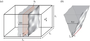
(a) Schematic set-up of the planar temporal plume, in contrast to the classical stationary spatially evolving flow (b). The sources of buoyancy are marked in red. For the temporal case, the initial buoyancy distribution
 $b_{0}(y)$
is given in (3.1).

2 Theory
2.1 Governing equations
The plume equations comprise conservation equations for volume, streamwise momentum and buoyancy. Within the Boussinesq approximation and for uniform background density
 $\unicode[STIX]{x1D70C}_{0}$
, this set is given by
 $$\begin{eqnarray}\displaystyle & \displaystyle \unicode[STIX]{x1D735}\boldsymbol{\cdot }\boldsymbol{u}=0, & \displaystyle\end{eqnarray}$$
 $$\begin{eqnarray}\displaystyle & \displaystyle \frac{\unicode[STIX]{x2202}w}{\unicode[STIX]{x2202}t}+\boldsymbol{u}\boldsymbol{\cdot }\unicode[STIX]{x1D735}w=-\frac{\unicode[STIX]{x2202}p}{\unicode[STIX]{x2202}z}+\unicode[STIX]{x1D708}\unicode[STIX]{x1D6FB}^{2}w+b, & \displaystyle\end{eqnarray}$$
 $$\begin{eqnarray}\displaystyle & \displaystyle \frac{\unicode[STIX]{x2202}b}{\unicode[STIX]{x2202}t}+\boldsymbol{u}\boldsymbol{\cdot }\unicode[STIX]{x1D735}b=\unicode[STIX]{x1D705}\unicode[STIX]{x1D6FB}^{2}b, & \displaystyle\end{eqnarray}$$
where
 $\boldsymbol{u}\equiv (u,v,w)$
denotes the velocity vector with components in the transverse, cross-stream and longitudinal directions respectively,
 $p$
is the kinematic pressure (with the hydrostatic balance subtracted),
 $\unicode[STIX]{x1D708}$
is the kinematic viscosity and
 $\unicode[STIX]{x1D705}$
is the buoyancy diffusivity. Further, the buoyancy force is given by
 $b\equiv g(\unicode[STIX]{x1D70C}_{0}-\unicode[STIX]{x1D70C})/\unicode[STIX]{x1D70C}_{0}$
, where
 $g$
is the gravitational acceleration and
 $\unicode[STIX]{x1D70C}$
denotes the local density.
2.2 Temporal plumes
The basic concept of the temporal plume is shown in figure 1(a). Unlike in the classical case where the flow evolves in space (i.e. along the streamwise coordinate
 $z$
, see figure 1
b), the mean-flow state in the temporal plume is only a function of time
 $t$
. Especially for a study targeting the dynamics in the vicinity of the TNTI, this set-up is advantageous since all averages can simply be taken across the entire numerical domain without the need to account for different mean-flow states, since
 $z$
and
 $x$
are homogeneous directions. In addition, there are numerical benefits from being able to employ a spectrally accurate code with triply periodic boundary conditions. It is for the same reasons that temporally evolving flows have been quite popular in the numerical study of the TNTI in momentum-driven flows (Bisset, Hunt & Rogers Reference Bisset, Hunt and Rogers2002; Mathew & Basu Reference Mathew and Basu2002; da Silva & Pereira Reference da Silva and Pereira2008; van Reeuwijk & Holzner Reference van Reeuwijk and Holzner2014).
We start the flow from a thin initial buoyancy distribution that is homogeneous in the
 $x$
- and
 $z$
-directions (see § 3.1 for details). Along with the periodic boundary conditions in all directions, this implies that for the mean field, only gradients with respect to the cross-stream (
 $y$
-) direction can be non-zero. Defining an average over the two homogeneous directions (
 $x$
and
 $z$
) such that, e.g.,
 $w(\boldsymbol{x},t)=\overline{w}(y,t)+w^{\prime }(\boldsymbol{x},t)$
, it immediately follows from (2.1) that
 $\overline{v}=\text{const.}=0$
. The averaged equation for the streamwise momentum equation reads
 $$\begin{eqnarray}\frac{\unicode[STIX]{x2202}\overline{w}}{\unicode[STIX]{x2202}t}+\frac{\unicode[STIX]{x2202}\overline{v^{\prime }w^{\prime }}}{\unicode[STIX]{x2202}y}=\unicode[STIX]{x1D708}\frac{\unicode[STIX]{x2202}^{2}\overline{w}}{\unicode[STIX]{x2202}y^{2}}+\overline{b}\end{eqnarray}$$
and the mean scalar transport equation is given by
 $$\begin{eqnarray}\frac{\unicode[STIX]{x2202}\overline{b}}{\unicode[STIX]{x2202}t}+\frac{\unicode[STIX]{x2202}\overline{v^{\prime }b^{\prime }}}{\unicode[STIX]{x2202}y}=\unicode[STIX]{x1D705}\frac{\unicode[STIX]{x2202}^{2}\overline{b}}{\unicode[STIX]{x2202}y^{2}}.\end{eqnarray}$$
As we show in appendix A, there exists an analogy between temporal flows and spatially evolving jets and plumes in a strong coflow. Hence, a flow described by (2.4) and (2.5) can also be realized in experiments.
Both the flow and the scalar concentration are zero far away from the centreline of the plume. Therefore, it follows from integrating (2.5) along the cross-stream direction (
 $y$
) that the total buoyancy content in a cross-section of the flow is conserved, i.e.
 $$\begin{eqnarray}\int _{-\infty }^{\infty }\overline{b}\,\text{d}y\equiv B=\text{const.},\end{eqnarray}$$
which has dimensions of velocity squared. Integration of (2.4) along
 $y$
results in
 $$\begin{eqnarray}\int _{-\infty }^{\infty }\frac{\unicode[STIX]{x2202}\overline{w}}{\unicode[STIX]{x2202}t}\,\text{d}y=\int _{-\infty }^{\infty }\overline{b}\,\text{d}y,\end{eqnarray}$$
which can be integrated in time to obtain the volume flux
 $$\begin{eqnarray}Q\equiv \int _{-\infty }^{\infty }\overline{w}\,\text{d}y=Bt,\end{eqnarray}$$
where the integration constant is zero since
 $\overline{w}(t=0)=0$
. A Reynolds number based on the volume flux can then be formed by
 $$\begin{eqnarray}Re=\frac{Bt}{\unicode[STIX]{x1D708}}.\end{eqnarray}$$
For
 $Re\rightarrow \infty$
(and fixed
 $Pr\equiv \unicode[STIX]{x1D708}/\unicode[STIX]{x1D705}$
), the viscous and diffusive terms become negligible and the only remaining relevant parameters in the temporal problem are a velocity scale
 $w^{\star }$
, a cross-stream length scale
 $l^{\star }$
and a buoyancy scale
 $b^{\star }$
. Equation (2.6) imposes the condition that
 $b^{\star }l^{\star }\propto B=\text{const.}$
Dimensional arguments then provide the scaling
 $$\begin{eqnarray}w^{\star }\propto \sqrt{B},\quad l^{\star }\propto t\sqrt{B},\quad b^{\star }\propto \frac{\sqrt{B}}{t}.\end{eqnarray}$$
Employing ‘top-hat’ scales (named after the implied top-hat shape of the distribution and indicated by
 $(\,\hat{\cdot }\,)$
throughout the paper) defined by
 $$\begin{eqnarray}Q={\hat{w}}\hat{l},\quad M\equiv \int _{-\infty }^{\infty }\overline{w}^{2}\,\text{d}y={\hat{w}}^{2}\hat{l},\quad B=\hat{b}\hat{l}\end{eqnarray}$$
and noting that if
 $Q(t=0)=0$
(as is the case in the simulations presented here) the integral constraint (2.8) implies that no virtual origin correction is required allows us to restate (2.10) as
 $$\begin{eqnarray}{\hat{w}}=k_{w}\sqrt{B},\quad \hat{l}=k_{l}t\sqrt{B},\quad \hat{b}=\frac{k_{g}\sqrt{B}}{t}.\end{eqnarray}$$
By means of (2.6) and (2.8), the set of three constants can be reduced to a single independent parameter
 $k_{l}$
according to
 $$\begin{eqnarray}k_{w}=k_{g}=\frac{1}{k_{l}}.\end{eqnarray}$$
As an aside, we consider the scaling for laminar flow. In this case,
 $Re\rightarrow 0$
, which implies that the turbulent-inertia term in (2.4) vanishes while the viscous contribution is retained. The integral constraint in (2.6) remains unchanged, and replacing the turbulent time scale by a viscous one leads to the laminar scaling given by
 $$\begin{eqnarray}w_{lam}^{\star }\propto \frac{B}{\sqrt{\unicode[STIX]{x1D708}}}t^{1/2},\quad l_{lam}^{\star }\propto \sqrt{\unicode[STIX]{x1D708}}t^{1/2},\quad b_{lam}^{\star }\propto \frac{B}{\sqrt{\unicode[STIX]{x1D708}}}t^{-1/2},\end{eqnarray}$$
noting that for consistency with (2.12),
 $l_{lam}^{\star }$
is a length scale based on the velocity distribution only.
2.3 Entrainment
Considering the situation at an integral level, the two integral equations (2.6) and (2.8) are not sufficient to solve for the three unknowns
 $Q$
,
 $M$
and
 $B$
. In the spatially evolving case, the set of equations is closed by introducing an entrainment relation on the right-hand side of the integral continuity equation (e.g. Morton et al.
Reference Morton, Taylor and Turner1956). For the temporal plume, however, the continuity equation vanishes since it does not feature a temporal derivative, i.e. we have
 $\unicode[STIX]{x2202}Q/\unicode[STIX]{x2202}z=0$
. Yet, it is possible to define an analogous entrainment relation for the temporal spreading of the flow by considering
 $$\begin{eqnarray}\frac{\text{d}\hat{l}}{\text{d}t}=\frac{\text{d}}{\text{d}t}\left(\frac{Q^{2}}{M}\right)\equiv 2u_{e}\equiv 2\unicode[STIX]{x1D6FC}{\hat{w}},\end{eqnarray}$$
where
 $u_{e}$
is the bulk entrainment velocity and
 $\unicode[STIX]{x1D6FC}$
is the top-hat entrainment parameter. It should be noted that the factor 2 enters in (2.15) since entrainment occurs simultaneously at two fronts (cf. figure 1
a). By comparing (2.15) and (2.12), we identify the self-similar scaling constant as
 $$\begin{eqnarray}k_{l}=2\unicode[STIX]{x1D6FC}_{0}\frac{{\hat{w}}}{\sqrt{B}}=\sqrt{2\unicode[STIX]{x1D6FC}_{0}},\end{eqnarray}$$
where
 $\unicode[STIX]{x1D6FC}_{0}$
is the constant entrainment parameter in the self-similar state. Based on this relation, a flux-balance parameter in the vein of Morton (Reference Morton1959) can be defined as
 $$\begin{eqnarray}\unicode[STIX]{x1D6E4}=\frac{BQ^{2}}{2\unicode[STIX]{x1D6FC}_{0}M^{2}}.\end{eqnarray}$$
In the self-similar case,
 $BQ^{2}/M^{2}=k_{l}^{2}=2\unicode[STIX]{x1D6FC}_{0}$
, and the constant
 $1/(2\unicode[STIX]{x1D6FC}_{0})$
in (2.17) is chosen such that – analogous to the spatial case (Morton Reference Morton1959) –
 $\unicode[STIX]{x1D6E4}=1$
relates to a pure plume, whereas
 $\unicode[STIX]{x1D6E4}<1$
and
 $\unicode[STIX]{x1D6E4}>1$
signify forced plumes and lazy plumes respectively.
In the following, we will outline how the entrainment parameter
 $\unicode[STIX]{x1D6FC}$
can be determined from an integral framework as well as using an approach that is related to the local propagation of the turbulent/non-turbulent interface.
2.3.1 Integral entrainment analysis
In order to pinpoint the differences and simplifications in the temporal case, we start from the general set of equations (2.1)–(2.3) describing a non-stationary spatially evolving planar plume. After averaging (with the understanding that averaging is restricted to the homogeneous
 $x$
-direction as long as the spatial case is considered), we obtain
 $$\begin{eqnarray}\displaystyle & \displaystyle \frac{\unicode[STIX]{x2202}\overline{v}}{\unicode[STIX]{x2202}y}+\frac{\unicode[STIX]{x2202}\overline{w}}{\unicode[STIX]{x2202}z}=0, & \displaystyle\end{eqnarray}$$
 $$\begin{eqnarray}\displaystyle & \displaystyle \frac{\unicode[STIX]{x2202}\overline{w}}{\unicode[STIX]{x2202}t}+\frac{\unicode[STIX]{x2202}\overline{w}^{2}}{\unicode[STIX]{x2202}z}+\frac{\unicode[STIX]{x2202}(\overline{v}\,\overline{w})}{\unicode[STIX]{x2202}y}+\frac{\unicode[STIX]{x2202}\overline{v^{\prime }w^{\prime }}}{\unicode[STIX]{x2202}y}+\underbrace{\frac{\unicode[STIX]{x2202}\overline{w^{\prime 2}}}{\unicode[STIX]{x2202}z}}_{O(l/L)}=\underbrace{-\frac{\unicode[STIX]{x2202}\overline{p}}{\unicode[STIX]{x2202}z}}_{O(l/L)}+\unicode[STIX]{x1D708}\frac{\unicode[STIX]{x2202}^{2}\overline{w}}{\unicode[STIX]{x2202}y^{2}}+\overline{b}, & \displaystyle\end{eqnarray}$$
 $$\begin{eqnarray}\displaystyle & \displaystyle \frac{\unicode[STIX]{x2202}\overline{b}}{\unicode[STIX]{x2202}t}+\frac{\unicode[STIX]{x2202}(\overline{w}\overline{b})}{\unicode[STIX]{x2202}z}+\frac{\unicode[STIX]{x2202}(\overline{v}\overline{b})}{\unicode[STIX]{x2202}y}+\frac{\unicode[STIX]{x2202}\overline{v^{\prime }b^{\prime }}}{\unicode[STIX]{x2202}y}+\underbrace{\frac{\unicode[STIX]{x2202}\overline{w^{\prime }b^{\prime }}}{\unicode[STIX]{x2202}z}}_{O(l/L)}=\unicode[STIX]{x1D705}\frac{\unicode[STIX]{x2202}^{2}\overline{b}}{\unicode[STIX]{x2202}y^{2}}. & \displaystyle\end{eqnarray}$$
We note that
 $p$
is the kinematic pressure with the hydrostatic balance subtracted, such that from the
 $y$
-momentum equation it follows that
 $\unicode[STIX]{x2202}_{z}\overline{v^{\prime 2}}+\unicode[STIX]{x2202}_{z}\overline{p}=0$
, which is used to substitute for
 $\unicode[STIX]{x2202}_{z}\overline{v^{\prime 2}}$
in (2.19). As mentioned before, (2.18) vanishes upon integration in the temporal case. However, also for the spatial flow it is beneficial not to use volume conservation directly since it provides no additional information about the turbulence. Instead, the energy transport equation can be employed, which together with (2.19) and (2.20) provides a framework that is consistent with (2.18)–(2.20) (van Reeuwijk & Craske Reference van Reeuwijk and Craske2015).
The transport equation for the mean streamwise kinetic energy
 $\overline{w}^{2}$
is obtained by multiplying (2.19) by
 $2\overline{w}$
, which results in
 $$\begin{eqnarray}\displaystyle & & \displaystyle \displaystyle \frac{\unicode[STIX]{x2202}\overline{w}^{2}}{\unicode[STIX]{x2202}t}+\frac{\unicode[STIX]{x2202}\overline{w}^{3}}{\unicode[STIX]{x2202}z}+2\frac{\unicode[STIX]{x2202}(\overline{w}\overline{v^{\prime }w^{\prime }})}{\unicode[STIX]{x2202}y}+\overbrace{2\frac{\unicode[STIX]{x2202}(\overline{w}\overline{w^{\prime 2}})}{\unicode[STIX]{x2202}z}+2\frac{\unicode[STIX]{x2202}(\overline{w}\,\overline{p})}{\unicode[STIX]{x2202}z}}^{O(l/L)}\nonumber\\ \displaystyle & & \displaystyle \displaystyle \quad =\underbrace{2\frac{\unicode[STIX]{x2202}\overline{w}}{\unicode[STIX]{x2202}z}\overline{w^{\prime 2}}+2\frac{\unicode[STIX]{x2202}\overline{w}}{\unicode[STIX]{x2202}z}\overline{p}}_{O(l/L)}+2\frac{\unicode[STIX]{x2202}\overline{w}}{\unicode[STIX]{x2202}y}\overline{w^{\prime }v^{\prime }}+2\overline{w}\overline{b}+\unicode[STIX]{x1D708}\frac{\unicode[STIX]{x2202}^{2}\overline{w}^{2}}{\unicode[STIX]{x2202}y^{2}}-2\unicode[STIX]{x1D708}\left(\frac{\unicode[STIX]{x2202}\overline{w}}{\unicode[STIX]{x2202}y}\right)^{2}.\end{eqnarray}$$
At this point, it is instructive to inspect the terms in (2.19)–(2.21) that drop out in the temporally evolving flow. The temporal flow is homogeneous in the streamwise direction, which implies that
 $\unicode[STIX]{x2202}_{z}=0$
. Consequently, any longitudinal transport terms are absent in the temporal case. An examination of the terms associated with
 $\unicode[STIX]{x2202}_{z}(\cdot )$
in (2.19)–(2.21) shows that most of them are
 $O(l/L)$
with respect to leading order, where
 $L$
and
 $l$
denote longitudinal and transverse length scales respectively. Terms of this order are also commonly neglected for
 $Re\rightarrow \infty$
in the classical theory for spatial flows (cf. Tennekes & Lumley (Reference Tennekes and Lumley1994), even though Craske & van Reeuwijk (Reference Craske and van Reeuwijk2015) point out that the underlying assumption of
 $l/L\rightarrow 0$
is questionable). However, each transport equation also features one longitudinal transport term (the second term on the left-hand side in each case) that is of leading order. It seems therefore reasonable to expect the bulk flow to behave differently from the spatial case. This statement naturally also applies to temporally evolving jets, even though this disclosure is not commonly made in the literature (e.g. da Silva & Pereira Reference da Silva and Pereira2008; Taveira & da Silva Reference Taveira and da Silva2013).
We will restrict the following discussion to the temporal flow and refer the reader to Craske & van Reeuwijk (Reference Craske and van Reeuwijk2016), whose notation we follow, for a detailed analysis of the unsteady spatial case. A discussion of the steady spatial flow is included in appendix B. Integrating (2.19)–(2.21) over the cross-stream direction and using the fact that the streamwise derivative vanishes in the mean for the temporal flow results in
 $$\begin{eqnarray}\displaystyle & \displaystyle \frac{\text{d}}{\text{d}t}B=0, & \displaystyle\end{eqnarray}$$
 $$\begin{eqnarray}\displaystyle & \displaystyle \frac{\text{d}}{\text{d}t}Q=B, & \displaystyle\end{eqnarray}$$
 $$\begin{eqnarray}\displaystyle & \displaystyle \frac{\text{d}}{\text{d}t}M=2\unicode[STIX]{x1D703}\frac{MB}{Q}+2\unicode[STIX]{x1D6FF}\frac{M^{3}}{Q^{3}}, & \displaystyle\end{eqnarray}$$
where
 $$\begin{eqnarray}\unicode[STIX]{x1D703}=\frac{Q}{MB}\int _{-\infty }^{\infty }\overline{w}\,\overline{b}\,\text{d}y\quad \text{and}\quad \unicode[STIX]{x1D6FF}=\frac{Q^{3}}{M^{3}}\int _{-\infty }^{\infty }\frac{\unicode[STIX]{x2202}\overline{w}}{\unicode[STIX]{x2202}y}\overline{v^{\prime }w^{\prime }}\,\text{d}y.\end{eqnarray}$$
It should be noted that in practice the integration limits have to replaced by finite values (
 $\pm L_{y}/2$
in our case). This is consistent as long as it is ensured that flow and buoyancy are negligible at the integration limits and beyond. We verified that this condition is met by the present simulations (see § 3.1).
Starting from the entrainment relation introduced in (2.15) and expanding the derivative results in
 $$\begin{eqnarray}\frac{\text{d}\hat{l}}{\text{d}t}=\frac{\text{d}}{\text{d}t}\left(\frac{Q^{2}}{M}\right)=2\frac{Q}{M}\frac{\text{d}Q}{\text{d}t}-\frac{Q^{2}}{M^{2}}\frac{\text{d}M}{\text{d}t}.\end{eqnarray}$$
Using (2.23) and (2.24) to eliminate the temporal derivatives on the right-hand side and upon comparison with (2.15), we arrive at
 $$\begin{eqnarray}\unicode[STIX]{x1D6FC}_{i}=-\unicode[STIX]{x1D6FF}+\left(1-\unicode[STIX]{x1D703}\right)Ri,\end{eqnarray}$$
where the plume Richardson number is given by
 $$\begin{eqnarray}Ri\equiv \frac{\hat{b}\hat{l}}{{\hat{w}}^{2}}=\frac{Q^{2}B}{M^{2}}=2\unicode[STIX]{x1D6FC}_{0}\unicode[STIX]{x1D6E4}.\end{eqnarray}$$
The physical significance of the first term on the right-hand side of (2.27), i.e. the production term written in (2.25b
), is straightforward: if mean kinetic energy is reduced by transfer to the field of fluctuations, the only way to conserve momentum is by adding volume to the flow (cf. 2.26). Since
 $Ri=0$
in the absence of buoyancy,
 $\unicode[STIX]{x1D6FF}$
is the only relevant term in temporal jets. The second term on the right-hand side of (2.27) represents the buoyancy contribution, which is best studied when restated as
 $$\begin{eqnarray}\unicode[STIX]{x1D6FC}_{i,b}\equiv \left(1-\unicode[STIX]{x1D703}\right)Ri=\frac{1}{{\hat{w}}^{3}}\left(\frac{M}{Q}B-\int _{-\infty }^{\infty }\overline{w}\,\overline{b}\,\text{d}y\right).\end{eqnarray}$$
Analogous to the discussion of the spatial case in van Reeuwijk & Craske (Reference van Reeuwijk and Craske2015), the first term of the difference is related to the
 $\text{d}Q/\text{d}t$
term on the right-hand side of (2.26). Positive changes of
 $Q$
lead to entrainment, and hence this buoyancy contribution to the entrainment coefficient is positive. The second term on the right-hand side of (2.26) comes with a minus sign, and accordingly the increase of
 $M$
(mean kinetic energy) due to the mean buoyancy flux leads to a negative contribution to
 $\unicode[STIX]{x1D6FC}$
. As (2.29) shows, the net effect of buoyancy in the temporal case is simply the difference of the two normalized by
 ${\hat{w}}^{3}$
. Stating the mean distributions
 $\overline{w}$
and
 $\overline{b}$
as
 $\overline{w}(y)={\hat{w}}S_{w}(y)$
and
 $\overline{b}(y)=\hat{b}S_{b}(y)$
, where
 $S_{w}$
and
 $S_{b}$
are dimensionless shape functions, the right-hand side of (2.29) can be expressed as
 $$\begin{eqnarray}\unicode[STIX]{x1D6FC}_{i,b}=\frac{\hat{b}\hat{l}}{\displaystyle {\hat{w}}^{2}}\left(\frac{\displaystyle \int _{-\infty }^{-\infty }S_{w}^{2}\,\text{d}(y/\hat{l})\int _{-\infty }^{-\infty }S_{b}\,\text{d}(y/\hat{l})}{\displaystyle \int _{-\infty }^{-\infty }S_{w}\,\text{d}(y/\hat{l})}-\int _{-\infty }^{-\infty }S_{b}S_{w}\,\text{d}(y/\hat{l})\right),\end{eqnarray}$$
and it becomes obvious that the difference in the brackets is 0 if
 $S_{w}=S_{b}$
. Hence, the buoyancy contribution can only be non-zero if the distributions of
 $\overline{b}$
and
 $\overline{w}$
have different shapes. For pure plumes at high
 $Re$
(and fixed
 $Pr$
), the velocity distribution is a direct consequence of the buoyancy distribution. By inspection of (2.4) and (2.5), a difference in the shapes of
 $\overline{b}$
and
 $\overline{w}$
can only be sustained in this case by the turbulent spanwise transport terms
 $\unicode[STIX]{x2202}_{y}\overline{v^{\prime }w^{\prime }}$
and
 $\unicode[STIX]{x2202}_{y}\overline{b^{\prime }v^{\prime }}$
. This is in contrast to the result for spatial plumes, where van Reeuwijk & Craske (Reference van Reeuwijk and Craske2015) find that even a hypothetical plume without turbulence would entrain. This fundamental discrepancy between spatial and temporal plumes originates from the fact that in the spatial flow buoyancy additionally affects the streamwise transport of momentum and energy. This results in a modification of the net-buoyancy contribution (see appendix B for the integral analysis in the spatial case) that is absent in the temporal case.
It is important to recall that (2.27) is in essence a constraint that ensures consistency with conservation of volume, momentum and energy (van Reeuwijk & Craske Reference van Reeuwijk and Craske2015). As such, the integral relation provides no information as to the detailed physical mechanisms that are causing entrainment. In the next section, we will therefore outline a different approach. Instead of inferring entrainment indirectly from bulk flow quantities, we will focus on the physical processes that give rise to entrainment locally.
2.3.2 Local analysis
It has long been known that in partly turbulent flows such as jets and plumes, regions of turbulent flow are bounded by a relatively sharp interface. In a local sense, entrainment can thus be interpreted as the movement of this boundary relative to the fluid. It is widely accepted that such a boundary can suitably be defined by using an appropriate threshold on enstrophy
 $\unicode[STIX]{x1D714}^{2}=\unicode[STIX]{x1D714}_{i}\unicode[STIX]{x1D714}_{i}$
(Bisset et al.
Reference Bisset, Hunt and Rogers2002; Holzner et al.
Reference Holzner, Liberzon, Nikitin, Lüthi, Kinzelbach and Tsinober2008; da Silva & Pereira Reference da Silva and Pereira2008; Wolf et al.
Reference Wolf, Lüthi, Holzner, Krug, Kinzelbach and Tsinober2012; van Reeuwijk & Holzner Reference van Reeuwijk and Holzner2014), where
 $\unicode[STIX]{x1D714}_{i}$
is the vorticity vector. Other definitions, e.g. using a passive scalar (Westerweel et al.
Reference Westerweel, Fukushima, Pedersen and Hunt2009) or turbulent kinetic energy (Philip et al.
Reference Philip, Meneveau, de Silva and Marusic2014), exist but are mostly limited to experimental studies where the velocity gradient tensor is not readily available. Conceptually, the choice of enstrophy is appealing since it naturally divides the flow into turbulent (vortical) and non-turbulent (non-vortical) regions. Practically, the fact that enstrophy is found to exhibit a sharp jump across the TNTI is advantageous as it renders the interface location rather insensitive to the exact threshold value for a wide range of thresholds.
Once a threshold is chosen (see § 5.2 for details), the local entrainment velocity
 $v_{n}$
can be defined as the movement of an enstrophy isosurface relative to the fluid. Following Holzner & Lüthi (Reference Holzner and Lüthi2011), this quantity can be computed from
 $$\begin{eqnarray}v_{n}\equiv -\frac{1}{\left|\unicode[STIX]{x1D735}\unicode[STIX]{x1D714}^{2}\right|}\frac{\text{D}\unicode[STIX]{x1D714}^{2}}{\text{D}t}.\end{eqnarray}$$
Using the enstrophy transport equation,
 $v_{n}$
can be decomposed according to
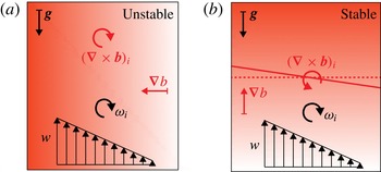
 $$\begin{eqnarray}v_{n}=\underbrace{-\frac{2\unicode[STIX]{x1D714}_{i}\unicode[STIX]{x1D714}_{j}s_{ij}}{\left|\unicode[STIX]{x1D735}\unicode[STIX]{x1D714}^{2}\right|}}_{v_{n}^{{\mathcal{I}}}}\underbrace{-\frac{\unicode[STIX]{x1D708}\unicode[STIX]{x1D6FB}^{2}\unicode[STIX]{x1D714}_{i}^{2}}{\left|\unicode[STIX]{x1D735}\unicode[STIX]{x1D714}^{2}\right|}}_{v_{n}^{{\mathcal{D}}}}\underbrace{+\frac{2\unicode[STIX]{x1D708}\left(\unicode[STIX]{x1D735}\unicode[STIX]{x1D714}_{i}\right)^{2}}{\left|\unicode[STIX]{x1D735}\unicode[STIX]{x1D714}^{2}\right|}}_{v_{n}^{{\mathcal{E}}}}\underbrace{-\frac{2\unicode[STIX]{x1D714}_{i}(\unicode[STIX]{x1D735}\times \boldsymbol{b})_{i}}{\left|\unicode[STIX]{x1D735}\unicode[STIX]{x1D714}^{2}\right|}}_{v_{n}^{{\mathcal{B}}}},\end{eqnarray}$$
where
 $\boldsymbol{b}=-b\tilde{\boldsymbol{g}}$
and
 $\tilde{\boldsymbol{g}}$
is the unit vector in the direction of gravity. In the order of their appearance, the terms on the right-hand side of (2.32) are associated with the physical mechanisms of inviscid vortex stretching (
 $v_{n}^{{\mathcal{I}}}$
), viscous diffusion (
 $v_{n}^{{\mathcal{D}}}$
) and destruction (
 $v_{n}^{{\mathcal{E}}}$
) of enstrophy, and the baroclinic torque (
 $v_{n}^{{\mathcal{B}}}$
). The latter term represents an interaction between the active scalar and the vorticity field.
The total volume flux
 $F_{\unicode[STIX]{x1D714}}$
through an instantaneous enstrophy isosurface
 $A_{\unicode[STIX]{x1D702}}$
is given by the integral
 $$\begin{eqnarray}F_{\unicode[STIX]{x1D714}}\equiv \int _{A_{\unicode[STIX]{x1D702}}}v_{n}\,\text{d}A=\langle v_{n}\rangle A_{\unicode[STIX]{x1D702}},\end{eqnarray}$$
where
 $\langle \cdot \rangle$
is an average over the isosurface. Hence, apart from the local entrainment velocity,
 $F_{\unicode[STIX]{x1D714}}$
also critically depends on the surface area of the enstrophy isosurface. In defining the rate at which fluid crosses the TNTI,
 $F_{\unicode[STIX]{x1D714}}$
is already an important quantity by itself. This is even more true as bounding the flow by the TNTI removes some of the arbitrariness associated with other choices such as the velocity half-width or a top-hat scale.
In order to be able to compare findings in the local framework with more conventional entrainment metrics, a relation between
 $F_{\unicode[STIX]{x1D714}}$
and the entrained mass flux in a top-hat framework given by
 $$\begin{eqnarray}\hat{F}=u_{e}A_{0}=\unicode[STIX]{x1D6FC}{\hat{w}}A_{0}\end{eqnarray}$$
needs to be established. Here,
 $A_{0}$
denotes the projected surface area, i.e. the area of the
 $xz$
-plane of the numerical domain. Such a relationship can be derived based on the self-similarity of the flow (van Reeuwijk & Holzner Reference van Reeuwijk and Holzner2014). In this case,
 $$\begin{eqnarray}\frac{\hat{l}(t)}{l_{\unicode[STIX]{x1D714}}(t)}=\text{const.},\end{eqnarray}$$
where
 $l_{\unicode[STIX]{x1D714}}(t)$
is the mean distance between the enstrophy isosurfaces bounding the flow in
 $y$
at time
 $t$
. It is important to note that (2.35) only holds if the threshold is defined relative to some bulk enstrophy value, e.g. the top-hat enstrophy
 $\hat{\unicode[STIX]{x1D714}}^{2}$
, since in the temporal flow
 $\hat{\unicode[STIX]{x1D714}}^{2}\propto t^{-1}$
. Denoting the mean propagation velocity of the enstrophy isosurface relative to the fluid by
 $2u_{\unicode[STIX]{x1D714}}=\text{d}l_{\unicode[STIX]{x1D714}}/\text{d}t$
and taking the derivative of (2.35) with respect to time, we get from (2.15) that
 $$\begin{eqnarray}u_{e}=\frac{\hat{l}}{l_{\unicode[STIX]{x1D714}}}u_{\unicode[STIX]{x1D714}}.\end{eqnarray}$$
Multiplication of (2.36) with
 $A_{0}$
and noting that
 $u_{\unicode[STIX]{x1D714}}A_{0}=F_{\unicode[STIX]{x1D714}}$
, i.e. that the flux that
 $u_{\unicode[STIX]{x1D714}}$
drives across the projected surface area
 $A_{0}$
is equivalent to the one that is observed to pass the convoluted interface, yields the desired relation of the fluxes
 $$\begin{eqnarray}\hat{F}=\frac{\hat{l}}{l_{\unicode[STIX]{x1D714}}}F_{\unicode[STIX]{x1D714}}.\end{eqnarray}$$
As outlined in Krug et al. (Reference Krug, Holzner, Lüthi, Wolf, Kinzelbach and Tsinober2015), this result allows us to express the canonical entrainment constant in terms of quantities related to the turbulent/non-turbulent interface. By substituting (2.34) and (2.15) into (2.37), we can solve for the entrainment coefficient
 $$\begin{eqnarray}\unicode[STIX]{x1D6FC}_{l}=\frac{F_{\unicode[STIX]{x1D714}}}{{\hat{w}}A_{0}}\frac{\hat{l}}{l_{\unicode[STIX]{x1D714}}}=\frac{\langle v_{n}\rangle }{{\hat{w}}}\frac{A_{\unicode[STIX]{x1D702}}}{A_{0}}\frac{\hat{l}}{l_{\unicode[STIX]{x1D714}}}.\end{eqnarray}$$
The first two ratios of the final product in (2.38) describe the local propagation of the TNTI and its degree of convolution respectively. The ratio of
 $\hat{l}$
and
 $l_{\unicode[STIX]{x1D714}}$
solely appears to relate the flux across the TNTI to more customary top-hat metrics. As a concluding remark to this section, we would like to point out that the different subscripts on
 $\unicode[STIX]{x1D6FC}$
(i for integral in (2.27) and l for local in (2.38)) are only used to signify the way in which the entrainment coefficient was computed. They all refer to the same quantity as defined in (2.15).
3 Simulations
3.1 Design of the temporal plume simulations
An ideal planar spatial plume originates from a line source in space. The corresponding initial condition for the temporal flow is a buoyancy distribution in the form of an infinitely thin sheet in the streamwise–transverse plane. A practical limit on how thin the initial distribution can be made in the simulations is given by the requirement that the discontinuity in the scalar distribution must be resolved by enough grid points to ensure resolution-independent results. In the style of the jet simulations by da Silva & Pereira (Reference da Silva and Pereira2008), we chose an initial scalar distribution given by
 $$\begin{eqnarray}b_{0}(y)=\frac{1}{2}+\frac{1}{2}\tanh \left[\frac{H}{4\unicode[STIX]{x1D713}}\left(1-\frac{2|y|}{H}\right)\right],\end{eqnarray}$$
with
 $\unicode[STIX]{x1D713}/H=0.1$
. We define a top-hat width
 $\hat{l}_{0b}$
based on the cross-stream integrals of
 $b_{0}$
and
 $b_{0}^{2}$
as a reference scale for the initial buoyancy distribution. For the value of
 $\unicode[STIX]{x1D713}/H$
used here, this results in
 $\hat{l}_{0b}\approx 1.25H$
. With the grid spacing
 $\unicode[STIX]{x1D6E5}$
, we found
 $N_{0}\equiv \hat{l}_{0b}/\unicode[STIX]{x1D6E5}\gtrsim 6$
to be sufficient for grid independence. Periodic boundary conditions are employed in all directions and, following the simulations of temporal jets (e.g. da Silva & Pereira Reference da Silva and Pereira2008; van Reeuwijk & Holzner Reference van Reeuwijk and Holzner2014), the aspect ratio of the computational domain is set to
 $L_{y}=1.5L_{x}=1.5L_{z}$
. The spatial resolution
 $\unicode[STIX]{x1D6E5}$
is chosen to be the same in all directions. In order to force transition, random noise with a maximum amplitude of 4 % of the local scalar concentration is added to the scalar profile as well as all three velocity components in the initial sheet where
 $b_{0}(y)>0$
. Apart from the seeding noise, all velocities are set to zero initially. The direct numerical simulation (DNS) is performed using a modified version of the pseudospectral code described in Chung & Matheou (Reference Chung and Matheou2012) with the mean shear set to zero. A third-order Runge–Kutta scheme is employed for time integration. For the dealiasing, we chose a
 $p$
th-order Fourier exponential filter (Hou & Li Reference Hou and Li2007; Chung & Pullin Reference Chung and Pullin2009) of the form
 $$\begin{eqnarray}\unicode[STIX]{x1D70E}(\unicode[STIX]{x1D719})=\exp \left(-\unicode[STIX]{x1D6FC}(\unicode[STIX]{x1D719}/\unicode[STIX]{x1D6FD})^{p}\right),\end{eqnarray}$$
with
 $\unicode[STIX]{x1D719}=(k_{x}^{2}+k_{y}^{2}+k_{z}^{2})/(\unicode[STIX]{x03C0}/\unicode[STIX]{x1D6E5})^{2}$
, where
 $k_{i}$
denotes the wavenumber in the
 $i$
-direction and
 $p=18$
. The constants
 $\unicode[STIX]{x1D6FC}=36$
and
 $\unicode[STIX]{x1D6FD}=0.75$
are selected such that the initial drop-off of the filter response approximately coincides with
 $\sqrt{\unicode[STIX]{x1D719}}=2/3$
(
 $\unicode[STIX]{x1D70E}(\sqrt{\unicode[STIX]{x1D719}}=2/3)\approx 0.997$
and
 $\unicode[STIX]{x1D70E}(\sqrt{\unicode[STIX]{x1D719}}\approx 0.776)=0.5$
); thus, the filter dealiases with a smoothed cutoff at a threshold that is slightly larger than
 $2/3$
.
Once the basic layout of the simulation is fixed as described above, two independent parameters need to be chosen. One of them is the number of grid points
 $N_{y}=L_{y}/\unicode[STIX]{x1D6E5}$
, which determines the size of the simulation and in practice is limited by the available computing resources. The other one takes the form of an initial Reynolds number
 $Re_{0}=(\hat{l}_{0b}\sqrt{B})/\unicode[STIX]{x1D708}$
. The choice of
 $Re_{0}$
determines how resolved the simulation is, which can be quantified by
 $r_{max}\equiv \unicode[STIX]{x1D6E5}/\unicode[STIX]{x1D702}_{min}$
, where
 $\unicode[STIX]{x1D702}_{min}$
is the minimum Kolmogorov length scale encountered over the duration of the simulation. With the scaling of the temporal plume (cf. (2.12)) and
 $\unicode[STIX]{x1D700}\propto {\hat{w}}^{3}/\hat{l}$
, we can infer for the Kolmogorov length scale
 $\unicode[STIX]{x1D702}\equiv (\unicode[STIX]{x1D708}^{3}/\unicode[STIX]{x1D700})^{1/4}\propto t^{1/4}$
, and hence expect
 $\unicode[STIX]{x1D702}_{min}$
to occur just after transition to turbulence. However, the exact relationship must be obtained empirically. We use
 $Pr=1$
, such that
 $\unicode[STIX]{x1D702}_{min}$
also represents the smallest Batchelor scale of the scalar field.
A set of smaller simulations was run with varying
 $Re_{0}$
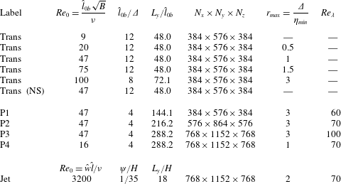
(see table 1 for details) in an effort to investigate the effect of different initial conditions on the transitional behaviour of the flow.
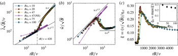
Results for the simulations performed to study the transitional behaviour of the flow (labelled ‘Trans’ in table 1). Panels (a,b) display the evolution of top-hat scales
 $\hat{l}$
and
 ${\hat{w}}$
. The Kolmogorov scale evaluated at the centreline is shown in (c); the inset plots the maximum value of
 $(\unicode[STIX]{x1D708}/\sqrt{B})/\unicode[STIX]{x1D702}_{cl}$
versus
 $Re_{0}$
. The legend in (a) applies to all panels; the case labelled ‘NS’ (open symbols) denotes a case without seeding. The dashed vertical lines in (a,b) indicate the start of the transition to turbulence at
 $Re_{crit}\approx 420$
. Also shown in (a,b) are the laminar growth rates for length (
 $t^{1/2}$
) and velocity (
 $t^{1/2}$
) and their counterparts in the turbulent regime (
 $\hat{l}\propto t^{1}$
and
 ${\hat{w}}\propto t^{0}$
).

Overview of all simulations analysed in the present study. For all plumes (labelled ‘Trans’ or ‘P’), we use
 $Pr=1$
and set
 $\unicode[STIX]{x1D713}/H=0.1$
which results in
 $\hat{l}_{0b}\approx 1.25H$
(see (3.1) and discussion thereof). The initial velocity distribution of the jet is of the same form as (3.1) using the parameters given in the table.

The results for these flows, which are labelled ‘Trans’ in table 1, are presented in figure 2. The evolution of the top-hat width and velocity in figure 2(a,b) clearly exhibits the transition from initially laminar flow with scalings according to (2.14) to the turbulent inviscid scaling given by (2.12). There is a good collapse for the data of plumes initiated with different
 $Re_{0}$
, which allows us to determine the Reynolds number at which transition starts empirically as
 $Re_{crit}\approx 420$
. A run with no seeding (marked with ‘NS’) does not transition and adheres to laminar scaling even beyond
 $Re_{crit}$
.
From figure 2(c), it can be concluded that
 $\unicode[STIX]{x1D709}_{0}\equiv \unicode[STIX]{x1D708}/(\sqrt{B}\unicode[STIX]{x1D702}_{min})\approx 0.3$
, with only a weak dependence on
 $Re_{0}$
. Based on this finding,
 $Re_{0}$
can be determined as a function of the resolution requirement
 $r_{max}=\unicode[STIX]{x1D6E5}/\unicode[STIX]{x1D702}_{min}$
from
 $$\begin{eqnarray}Re_{0}=\frac{\hat{l}_{0b}\sqrt{B}}{\unicode[STIX]{x1D708}}=\frac{N_{0}\unicode[STIX]{x1D6E5}\sqrt{B}}{\unicode[STIX]{x1D708}}=\frac{N_{0}r_{max}\unicode[STIX]{x1D702}_{min}\sqrt{B}}{\unicode[STIX]{x1D708}}=\frac{N_{0}}{\unicode[STIX]{x1D709}_{0}}r_{max}\approx \frac{6}{0.3}r_{max}=20r_{max}.\end{eqnarray}$$
According to (2.9), the bulk Reynolds number is proportional to
 $B$
and increases linearly with time. Hence, apart from the dependence on
 $Re_{0}$
, the maximum
 $Re$
that a simulation can reach is crucially determined by how long the flow can be considered to be free of confinement effects in the cross-stream direction. The onset of confinement is most easily detected from a deviation of the self-similar scaling of the bulk velocity where
 ${\hat{w}}\propto \text{const.}\,$
The domain-size effects are studied using a set of simulations where the box size and
 $Re_{0}$
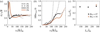
are systematically varied (cf. the simulations labelled P1–P4 in table 1). As figure 3(a) shows, all runs reach a self-similar state but depart from
 ${\hat{w}}\propto \text{const.}$
after some time. This departure generally occurs at later times for larger boxes (i.e. larger values of
 $L_{y}/\hat{l}_{0b}$
). The onset of the deviation is further accompanied by a significant increase in the level of root-mean-square cross-stream velocity fluctuations at the boundary of the domain (see figure 3
b), linking it to confinement effects. We define an approximate end of the proper scaling regime by visual inspection of figure 3(a) (marked by the transition from thick to thin lines). From figure 3(c), where the width
 $\hat{l}_{end}$
at this time is plotted, we find
 $\hat{l}_{end}\approx 0.3L_{y}$
as a criterion for the maximum width of the flow before boundary effects start to affect the simulation. This leads to the following empirical relation for the maximum Reynolds number:
 $$\begin{eqnarray}Re_{max}\equiv \frac{\hat{l}_{end}{\hat{w}}_{end}}{\unicode[STIX]{x1D708}}\approx \frac{\displaystyle 0.3L_{y}\frac{1}{k_{l}}\sqrt{B}}{\unicode[STIX]{x1D708}}=\frac{0.3N_{y}}{k_{l}N_{0}}Re_{0}=\frac{0.3}{k_{l}\unicode[STIX]{x1D709}_{0}}N_{y}r_{max}\approx 2.2N_{y}r_{max},\end{eqnarray}$$
where
 $1/k_{l}\approx 2.2$
(cf. figure 3
a) was used. It is noteworthy that (3.4) is more stringent than a requirement based on the instantaneous dynamical range, which would lead to
 $N_{y}\propto \hat{l}(t)/\unicode[STIX]{x1D702}(t)=Re^{3/4}$
. Since
 $\unicode[STIX]{x1D6E5}=\text{const.}$
, we need to resolve the range
 $\hat{l}(t)/\unicode[STIX]{x1D702}_{min}$
instead, which is proportional to
 $Re$
for the temporal plume.
(a) Top-hat velocity for simulations P1–P4 (see table 1 for details). (b) Root-mean-square value of streamwise velocity fluctuations at the boundary of the box (
 $y=0$
). (c) Top-hat width
 $\hat{l}_{end}$
at the end of the unconfined evolution (equivalent to the value at the end of the thick lines in (a)) plotted versus the dimensionless box size. The thin lines in (a,b) represent times where the flow is considered to be influenced by the finite size of the box.

3.2 Jet simulations
To allow for a comparison of some of our findings with results in a momentum-driven flow, we additionally ran a simulation of a temporal jet. This flow case is widely used in the literature (Bisset et al.
Reference Bisset, Hunt and Rogers2002; da Silva & Pereira Reference da Silva and Pereira2008; van Reeuwijk & Holzner Reference van Reeuwijk and Holzner2014) and will therefore only be discussed briefly here. Following da Silva & Pereira (Reference da Silva and Pereira2008), we choose an initial velocity profile of the same functional form as (3.1), setting
 $\unicode[STIX]{x1D713}/H=1/35$
. Just as in van Reeuwijk & Holzner (Reference van Reeuwijk and Holzner2014), the domain size here (see table 1 for details) is three times larger than the one used in da Silva & Pereira (Reference da Silva and Pereira2008). This allows for a much longer unconfined evolution of the flow, facilitating better convergence of turbulence statistics. In particular, we find that the larger box is a prerequisite for the entrainment parameter to attain an approximately constant value over at least a short timespan.
4 General flow statistics
In the following, we focus on the largest simulations P3 and P4, and refer to the jet simulation where appropriate. We use the reference time scales
 $$\begin{eqnarray}t^{\star }=\hat{l}_{0b}/\sqrt{B}\quad \text{for plumes and }t^{\star }=\hat{l}_{0}/(2{\hat{w}}_{0})~\text{for the jet }\end{eqnarray}$$
to normalize the computational time
 $t$
. For the simulation P4,
 $Re_{0}$
was chosen such that the minimum spatial resolution
 $\unicode[STIX]{x1D6E5}/\unicode[STIX]{x1D702}_{min}\approx 1$
, while for P3,
 $\unicode[STIX]{x1D6E5}/\unicode[STIX]{x1D702}_{min}\approx 3$
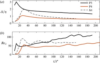
. As figure 4(a) shows, the relative resolution on the centreline improves quickly just after the transition of the flow. However, at later times, the additional gain from running the simulation for longer is only marginal since
 $\unicode[STIX]{x1D702}\propto t^{1/4}$
, as mentioned in § 3.1. At later stages of the flow evolution, P4 is very well resolved with
 $\unicode[STIX]{x1D6E5}/\unicode[STIX]{x1D702}\approx 0.6$
, while for P3
 $\unicode[STIX]{x1D6E5}/\unicode[STIX]{x1D702}\approx 1.5$
. In the jet,
 $\unicode[STIX]{x1D702}\propto t^{1/2}$
, and thus for this case (dashed line in figure 4
a) the resolution is seen to improve faster than for the plumes, reaching a level similar to P3.
The evolution of the Taylor–Reynolds number
 $Re_{\unicode[STIX]{x1D706}}$
is displayed in figure 4(b). We define
 $Re_{\unicode[STIX]{x1D706}}=(\overline{w_{cl}^{\prime 2}})^{1/2}\unicode[STIX]{x1D706}/\unicode[STIX]{x1D708}$
, with
 $\unicode[STIX]{x1D706}=(\overline{w_{cl}^{\prime 2}})^{1/2}/(\unicode[STIX]{x2202}_{z}\overline{w_{cl}^{\prime 2}})^{1/2}$
and the subscript
 $cl$
denoting quantities at the centreline of the flow where
 $y=0$
. Since
 $Re_{\unicode[STIX]{x1D706}}\propto Re^{1/2}$
(Pope Reference Pope2000), we find that
 $Re_{\unicode[STIX]{x1D706}}\propto (Bt)^{1/2}$
for the plume. Consistent with the
 $Re$
-criterion for transition, both plume simulations start from approximately the same value of
 $Re_{\unicode[STIX]{x1D706}}\approx 50$
after transition, from where
 $Re_{\unicode[STIX]{x1D706}}$
for P3 grows to reach
 $Re_{\unicode[STIX]{x1D706}}\approx 100$
by the end of the simulation. For P4, the maximum value is
 $Re_{\unicode[STIX]{x1D706}}\approx 70$
, which is approximately the same value as the one the jet attains. In the latter case,
 $Re=\text{const.}$
and hence also
 $Re_{\unicode[STIX]{x1D706}}$
is approximately constant once the flow has transitioned.
Spatial resolution at centreline (a) and
 $Re_{\unicode[STIX]{x1D706}}$
at centreline (b); the legend in (a) applies to both panels.

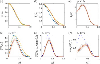
Self-similar profiles for P4 at different times, starting from
 $t/t^{\star }=100$
until
 $t/t^{\star }=200$
. The quantities plotted are (a) mean streamwise velocity
 $\overline{w}$
, (b) mean buoyancy
 $\overline{b}$
, (c) turbulent kinetic energy
 $k$
, (d) turbulent momentum flux
 $\overline{v^{\prime }w^{\prime }}$
, (e) turbulent production
 $\overline{v^{\prime }w^{\prime }}\unicode[STIX]{x2202}\overline{w}/\unicode[STIX]{x2202}y$
and (f) buoyant production of turbulent kinetic energy
 $\overline{b^{\prime }w^{\prime }}$
. Individual profiles are represented by grey lines and the mean over the entire timespan is plotted in red. The additional red lines in (e,f) correspond to means taken for
 $100<t/t^{\star }<150$
(dotted) and
 $150<t/t^{\star }<200$
(dashed). Shown as symbols in (a) and (d–f) are experimental data from plane spatial plumes by Ramaprian & Chandrasekhara (Reference Ramaprian and Chandrasekhara1989) (blue triangles) and Paillat & Kaminski (Reference Paillat and Kaminski2014) (yellow circles). All profiles are plotted using the respective symmetry with respect to the centre plane
 $y=0$
.

Mean profiles of the streamwise velocity
 $\overline{w}$
and buoyancy
 $\overline{b}$
are presented in figures 5(a) and 5(b) respectively. We plot these quantities for P4 in the range
 $100<t/t^{\star }<200$
normalized by the respective value at the centreline and the top-hat width
 $\hat{l}$
. The very good collapse of the profiles establishes self-similar behaviour of the flow beyond
 $t/t^{\star }=100$
. Naturally, higher-order statistics such as the turbulent kinetic energy (TKE)
 $k=(\overline{u^{\prime 2}+v^{\prime 2}+w^{\prime 2}})/2$
plotted in figure 5(c) or the turbulent momentum flux
 $\overline{v^{\prime }w^{\prime }}$
(5
d) are not equally well converged from a single snapshot. Consequently, the grey lines display somewhat more scatter for these quantities. The profiles nevertheless convincingly verify self-similarity for these quantities as well. The same is found to be true for the shear production of TKE,
 $\overline{v^{\prime }w^{\prime }}\unicode[STIX]{x2202}\overline{w}/\unicode[STIX]{x2202}y$
, and the buoyant production of TKE,
 $\overline{w^{\prime }b^{\prime }}$
, in figures 5(e) and 5(f) respectively. The profiles for
 $\overline{w}$
compare favourably with experimental data of spatially evolving planar plumes by Ramaprian & Chandrasekhara (Reference Ramaprian and Chandrasekhara1989) and Paillat & Kaminski (Reference Paillat and Kaminski2014), and the ones for
 $\overline{b}$
lie within the experimental scatter. However, the turbulence quantities in figure 5(d–f) appear to be consistently lower near the centreline of the temporal plume compared with the experimental data. Temporal averages taken separately for the first (dotted line) and second halves (dashed line) for the data in figure 5(e–f) show no conclusive trend and therefore rule out a temporal drift as a possible cause for the slight discrepancy. van Reeuwijk & Holzner (Reference van Reeuwijk and Holzner2014) cite a persistent dependence on initial conditions leading to non-universal behaviour as a potential reason for a similar observation when comparing temporal and spatial jet flows (even though, in contrast to the present case, TKE is overpredicted from the temporal simulation for the case without buoyancy). The fact that results from P3 (not shown) are slightly closer to the laboratory results might support this reasoning. At the same time, it cannot be ruled out that these differences in the turbulence statistics are genuine features of temporal flows.
5 Entrainment
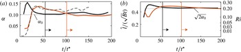
We begin by considering the temporal spreading of the flow. In figure 6, we plot the entrainment coefficient directly from its definition
 $\unicode[STIX]{x1D6FC}=(1/2){\hat{w}}^{-1}\,\text{d}\hat{l}/\text{d}t$
(figure 6
a) along with the spreading parameter
 $\hat{l}/(\sqrt{B}t)$
(figure 6
b). After an initial transient, the entrainment parameter
 $\unicode[STIX]{x1D6FC}$
attains an approximately constant value for P3 as well as P4. Despite the difference in Reynolds numbers between P3 and P4, both simulations tend to roughly the same value of
 $\unicode[STIX]{x1D6FC}_{0}\approx 0.1$
, recalling that the subscript ‘0’ is used to denote quantities in the self-similar state. A similar observation can be made from the plot of
 $\hat{l}/(\sqrt{B}t)$
, which according to (2.12) equals the scaling constant
 $k_{l}$
in the self-similar range. Once self-similarity is reached, both plumes approach a value that is equal to
 $\sqrt{2\unicode[STIX]{x1D6FC}_{0}}$
, as predicted by the relation (2.16). The results for
 $\unicode[STIX]{x1D6FC}$
and
 $k_{l}$
also provide further evidence that both plume simulations reach a sustained self-similar flow state that is unaffected by boundary effects. Additionally, figure 6(a) also includes data from the jet simulation. Also in this case, an approximately constant value of
 $\unicode[STIX]{x1D6FC}$
arises for the later stages of the flow evolution, as expected. Interestingly, the value of
 $\unicode[STIX]{x1D6FC}_{0}$
is observed to be slightly higher for the temporal jet than for the temporal plumes.
(a) Entrainment parameter
 $\unicode[STIX]{x1D6FC}$
determined from (2.15); (b)
 $k_{l}=\hat{l}/(\sqrt{B}t)$
plotted versus time; P3, black solid lines; P4, red solid lines; jet, dashed black line; vertical lines indicate the approximate start of self-similar flow for P3 (black) and P4 (red). The dotted horizontal lines are plotted using
 $\unicode[STIX]{x1D6FC}_{0}=0.102\,$
, which is the averaged mean value of P3 and P4 in the self-similar regime. It should be noted that the
 $Ri$
-axis on the right-hand side of (b) is on a quadratic scale.

5.1 Integral approach
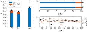
The results on the entrainment analysis at an integral level are compiled in figure 7. The bar plot in figure 7(a) shows the mean contributions of
 $-\unicode[STIX]{x1D6FF}$
(blue) and
 $(1-\unicode[STIX]{x1D703})Ri$
(red) for self-similar flow separately. The derivation leading to the expression for
 $\unicode[STIX]{x1D6FC}_{i}$
in (2.27) does not require any assumptions, and hence the good agreement of
 $\unicode[STIX]{x1D6FC}_{i,0}$
and
 $\unicode[STIX]{x1D6FC}_{0}$
(diamonds) is to be expected, as discrepancies can arise only from numerical errors and insufficient convergence of the integrals. Even though the absolute values for
 $\unicode[STIX]{x1D6FC}_{0}$
and consistently those of
 $\unicode[STIX]{x1D6FC}_{i,0}$
differ slightly between P3 and P4, the relative contribution of
 $\unicode[STIX]{x1D6FC}_{i,b}$
to
 $\unicode[STIX]{x1D6FC}_{i,0}$
is almost identical in both simulations at approximately 15 % (cf. figure 7
b).
For pure plumes,
 $\unicode[STIX]{x1D6E4}=1$
by definition, and from (2.28) it then follows that
 $Ri=2\unicode[STIX]{x1D6FC}_{0}\approx 0.2$
. This value is attained relatively quickly after transition of the flow, as can be seen from figure 6(b) (quadratic
 $Ri$
-axis on the right-hand side). The value of
 $Ri$
represents a theoretical upper bound for
 $\unicode[STIX]{x1D6FC}_{i,0}$
in the case that
 $\unicode[STIX]{x1D703}=0$
, which would, however, require the distributions of
 $\overline{w}$
and
 $\overline{b}$
to be completely uncorrelated, i.e.
 $\int _{-\infty }^{\infty }S_{w}S_{b}\,\text{d}(y/\hat{l})=0$
. Practically, of course, the mean velocity profile is a direct consequence of the action of buoyancy, and the decorrelation due to differences in turbulent transport is rather weak. Hence, we find
 $(1-\unicode[STIX]{x1D703})\approx 0.1$
, which leads to the small buoyancy contribution compared with
 $\unicode[STIX]{x1D6FF}$
. Referring to figure 7(c), we note further that the value of
 $\unicode[STIX]{x1D6FC}_{i,b}/\unicode[STIX]{x1D6FC}_{i}\approx 0.15$
is quite robust. This is true even at early stages of the evolution of the plumes where, from figure 6,
 $\unicode[STIX]{x1D6FC}$
and
 $\unicode[STIX]{x1D6E4}$
are quite different from their self-similar values. Also plotted in figure 7(c) is
 $1/{\hat{w}}^{3}\int \overline{b^{\prime }w^{\prime }}\,\text{d}y$
(dashed lines), which represents the production of turbulent kinetic energy due to buoyancy normalized by
 ${\hat{w}}^{3}$
. At all times and for both plume simulations, this quantity is seen to agree with
 $\unicode[STIX]{x1D6FC}_{i,b}$
to within approximately 5 %. It appears at least noteworthy that the difference on the right-hand side of (2.29) is numerically very close to the direct production of turbulent kinetic energy by buoyancy in our simulations. However, we have not been able to establish a direct relationship between the two, and the agreement may ultimately turn out to be coincidental.
(a) Results from the integral entrainment analysis (bars) compared with direct estimates (black diamonds) using (2.15); the open symbol refers to DNS of a temporal jet by van Reeuwijk & Holzner (Reference van Reeuwijk and Holzner2014) at
 $Re=5000$
. (b) Contributions to
 $\unicode[STIX]{x1D6FC}_{i}$
in per cent of the total
 $\unicode[STIX]{x1D6FC}$
. (c) Buoyancy contribution
 $\unicode[STIX]{x1D6FC}_{i,b}$
according to (2.29) relative to the overall entrainment coefficient
 $\unicode[STIX]{x1D6FC}$
as a function of time for P3 (black lines) and P4 (red lines); solid lines,
 $\unicode[STIX]{x1D6FC}_{i,b}$
according to (2.29); dashed lines,
 $1/{\hat{w}}^{3}\int \overline{b^{\prime }w^{\prime }}\,\text{d}y$
.

For the sake of completeness, we also show in figure 7(a) data from the integral analysis for the jet simulation, where the only contribution to
 $\unicode[STIX]{x1D6FC}_{i}$
is
 $\unicode[STIX]{x1D6FF}$
. This value is higher for the jet than for plumes, and even with the additional buoyancy contribution
 $\unicode[STIX]{x1D6FC}_{i}$
remains lower for the plumes, a fact that was already observed in the plot of
 $\unicode[STIX]{x1D6FC}$
in figure 6(a). This situation is the reverse to spatial flows, where it is commonly observed that pure plumes entrain more than jets. Moreover, there is a notion that
 $\unicode[STIX]{x1D6FF}$
is approximately equal in spatial jets and plumes (Kaminski et al.
Reference Kaminski, Tait and Carazzo2005; Carazzo, Kaminski & Tait Reference Carazzo, Kaminski and Tait2006; van Reeuwijk & Craske Reference van Reeuwijk and Craske2015), which is also clearly not the case for the present temporal data.
However, given the fundamental differences between temporally and spatially evolving flows that we discussed earlier (see the discussion in § 2.3.1), these differences do not imply that our results are at odds with previous experimental and numerical evidence. The observation that
 $\unicode[STIX]{x1D6FF}$
attains similar values in spatial plumes and jets is empirical only, and it is not compulsory that temporal flows would behave in the same manner.
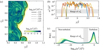
(a) Logarithmic contour plot of enstrophy; the black lines represent the different threshold values used. (b) Sample enstrophy profiles at different
 $z$
-positions; the grey-shaded area corresponds to the range of enstrophy thresholds. (c) Probability density function of
 $\log _{10}(\unicode[STIX]{x1D714}_{th}^{2}/\hat{\unicode[STIX]{x1D714}}^{2})$
at different times
 $60<t/t^{\star }<200$
, with
 $t$
increasing from light to dark green. Results are shown for P4 only.

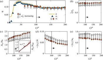
(a) Results for
 $\unicode[STIX]{x1D6FC}_{l}$
at different times and varying thresholds compared with
 $\unicode[STIX]{x1D6FC}_{i}$
and
 $\unicode[STIX]{x1D6FC}$
. (b) Ratio of
 $\hat{l}$
and the distance
 $l_{\unicode[STIX]{x1D714}}$
between the mean positions of the two enstrophy isosurfaces bounding the flow. (c) Surface area of the interface
 $A_{\unicode[STIX]{x1D702}}$
normalized by the base area of the numerical domain. The inset shows the same data plotted in log-scale and normalized by the value
 $A_{\unicode[STIX]{x1D702}0}=A_{\unicode[STIX]{x1D702}}(t/t^{\star }=100)$
for the respective threshold. For comparison, grey lines indicate scalings
 $\propto t^{1/3}$
and
 $\propto t^{1/5}$
. Panels (d–e) show the local entrainment velocity
 $\langle v_{n}\rangle$
averaged across the interface and normalized by
 ${\hat{w}}$
(d) and the Kolmogorov velocity
 $u_{\unicode[STIX]{x1D702}}$
(e). In all plots, open and filled symbols represent the lowest and highest threshold respectively. Results are shown for P4 only.

Finally, it should be noted that absolute values of
 $\unicode[STIX]{x1D6FC}$
from temporal simulations come with a caveat, since the dependence on initial conditions is known to decay slowly in these wake-like flows (Redford, Castro & Coleman Reference Redford, Castro and Coleman2012). The problem is most prevalent in the jet simulations, as evidenced by the result of van Reeuwijk & Holzner (Reference van Reeuwijk and Holzner2014) (open symbol in figure 7
a), who obtain a much higher
 $\unicode[STIX]{x1D6FC}$
at
 $Re=5000$
. Judging by the fact that results for P3 and P4 agree closely, the effect of initial conditions appears to be less persistent for the plume. Presumably, this is due to the active role that buoyancy plays in creating and sustaining the flow and turbulence in plumes in contrast to jets, which are more dependent on initial conditions. A similar suggestion was already put forward by Carazzo et al. (Reference Carazzo, Kaminski and Tait2006), who observed for spatial flows that plumes approach an asymptotic self-similar regime faster than jets.
5.2 Local approach
5.2.1 Detection of the interface
Figure 8(a) shows an enstrophy snapshot of a slice covering part of the numerical domain from simulation P4. The local enstrophy is normalized by
 $\hat{\unicode[STIX]{x1D714}}^{2}$
, which is defined in top-hat fashion by
 $$\begin{eqnarray}\hat{\unicode[STIX]{x1D714}}^{2}\equiv \frac{\displaystyle \int _{-\infty }^{\infty }(\overline{\unicode[STIX]{x1D714}^{2}})^{2}\text{d}y}{\displaystyle \int _{-\infty }^{\infty }\overline{\unicode[STIX]{x1D714}^{2}}\,\text{d}y}.\end{eqnarray}$$
It can be observed from the figure that the difference in enstrophy levels between the turbulent and non-turbulent regions of the flow is several orders of magnitude. This presents a wide range of choices for possible threshold values
 $\unicode[STIX]{x1D714}_{th}^{2}$
. In fact, in a recent study, van Reeuwijk & Holzner (Reference van Reeuwijk and Holzner2014) studied thresholds ranging from the turbulent core to very low thresholds in the essentially irrotational region. Here, we will restrict ourselves to values of
 $\unicode[STIX]{x1D714}_{th}^{2}$
that result in isosurfaces that form an ‘outer shell’ of the flow with only negligible detached regions inside the turbulent zone. From figure 8(a) and the sample enstrophy profiles in figure 8(b), we find that this is the case for
 $\log _{10}(\unicode[STIX]{x1D714}_{th}^{2}/\hat{\unicode[STIX]{x1D714}}^{2})\leqslant -2.5$
, which is the highest threshold value used in this study. In addition, we test four lower thresholds spanning a total range of two orders of magnitude down to
 $\log _{10}(\unicode[STIX]{x1D714}_{th}^{2}/\hat{\unicode[STIX]{x1D714}}^{2})=-4.5$
. Even lower thresholds are possible in principle, but we found that results are increasingly affected by numerical noise. The interface positions corresponding to each of the total of five thresholds used are marked by black lines in figure 8(a). To characterize the chosen thresholds in terms of the overall range of enstrophy values, the probability density function (p.d.f.) of
 $\log _{10}(\unicode[STIX]{x1D714}_{th}^{2}/\hat{\unicode[STIX]{x1D714}}^{2})$
at different times is plotted in figure 8(c). The values of
 $\unicode[STIX]{x1D714}_{th}^{2}$
are indicated by the shaded grey area, and the figure confirms that the chosen range bounds the peak corresponding to the region of turbulent flow from below at all times. Using
 $\unicode[STIX]{x1D700}\propto \unicode[STIX]{x1D708}\hat{\unicode[STIX]{x1D714}}^{2}$
, we find that the bulk enstrophy level in the plume scales with time according to
 $\hat{\unicode[STIX]{x1D714}}^{2}\propto t^{-1}$
. Defining the threshold value relative to
 $\hat{\unicode[STIX]{x1D714}}^{2}$
as is done here has the benefit of removing this time dependence from the interface detection criterion. A suggestion to this effect was already put forward in van Reeuwijk & Holzner (Reference van Reeuwijk and Holzner2014), even though they chose to normalize the thresholds using initial conditions in line with previous work (Bisset et al.
Reference Bisset, Hunt and Rogers2002; da Silva & Pereira Reference da Silva and Pereira2008).
5.2.2 Interface-based entrainment coefficient
The consistency of the local entrainment framework can be assessed by comparing the results for
 $\unicode[STIX]{x1D6FC}_{l}$
(2.38) with
 $\unicode[STIX]{x1D6FC}_{i}$
and
 $\unicode[STIX]{x1D6FC}$
as presented for P4 in figure 9(a). Indeed, very good agreement is observed for
 $t/t^{\star }\geqslant 100$
. This time roughly corresponds to the onset of self-similar flow behaviour, consistent with the fact that the derivation of (2.38) is based on self-similarity of the enstrophy profile. It is further noteworthy that the good correspondence between integral and locally derived entrainment parameters is obtained without any temporal averaging. This implies that the box size of the simulation is large enough for all relevant interface-related statistics to converge sufficiently. Ideally, the value of
 $\unicode[STIX]{x1D6FC}_{l}$
should be threshold-independent. In view of the large range of
 $\unicode[STIX]{x1D714}_{th}^{2}$
, the variation of
 $\unicode[STIX]{x1D6FC}_{l}$
appears to be in fact relatively small. Nevertheless, there is a systematic trend for
 $\unicode[STIX]{x1D6FC}_{l}$
to decrease slightly with decreasing
 $\unicode[STIX]{x1D714}_{th}^{2}$
, leading to a slight underprediction of
 $\unicode[STIX]{x1D6FC}_{l}$
at the smallest thresholds compared with
 $\unicode[STIX]{x1D6FC}_{i}$
and
 $\unicode[STIX]{x1D6FC}$
. A similar systematic error was observed in van Reeuwijk & Holzner (Reference van Reeuwijk and Holzner2014). These authors also showed that a mean local entrainment velocity computed from the change of turbulent volume does not feature this spurious trend. It is therefore likely to be related to numerical noise in the computation of
 $v_{n}$
. Indeed, capturing the interface propagation is quite a challenging problem numerically, and – similarly to related investigations (Holzner et al.
Reference Holzner, Song, Avila and Hof2013; van Reeuwijk & Holzner Reference van Reeuwijk and Holzner2014) – we find that matching locally obtained entrainment metrics to global ones requires very well resolved simulations even at the highest threshold. Concretely, the difference between
 $\unicode[STIX]{x1D6FC}_{l}$
and
 $\unicode[STIX]{x1D6FC}$
for the higher-
 $Re$
plume P3 is already of the order of 50 % for the highest threshold. The relative spatial resolution is coarser by approximately a factor of 2 for this case (cf. figure 4
a), so that achieving a resolution comparable to P4 would require eight times more grid points. This is beyond our current capabilities, and it was therefore decided to forgo P3 in the local analysis. In light of the fact that in the discussion of figures 6 and 7 we were already able to show that the general entrainment characteristics are in very good agreement for P3 and P4, this does not come at a great loss of significance.
Having established the agreement between
 $\unicode[STIX]{x1D6FC}_{l}$
and
 $\unicode[STIX]{x1D6FC}$
, we can now move on to investigate the factors in (2.38) individually. The ratio of length scales
 $\hat{l}/l_{\unicode[STIX]{x1D714}}$
was assumed to be constant in the derivation of (2.38). Figure 9(b) confirms this and thereby also the underlying assumption of self-similarity of the enstrophy profile for
 $t/t^{\star }>90$
. It is further interesting to note that the values of
 $\hat{l}/l_{\unicode[STIX]{x1D714}}$
are very close to 1. This is indicative of the fact that instantaneous flow profiles are well approximated by a top-hat distribution. Furthermore, having
 $\hat{l}/l_{\unicode[STIX]{x1D714}}\approx 1$
also implies that the entrained volume flux through the TNTI nearly equals the top-hat entrainment flux, i.e.
 $F_{\unicode[STIX]{x1D714}}\approx \hat{F}$
. In this sense, the top-hat distribution therefore appears to be a good representation of the flow.
5.2.3 Surface area of the TNTI
While the factor
 $\hat{l}/l_{\unicode[STIX]{x1D714}}$
merely appears in (2.38) to relate
 $F_{\unicode[STIX]{x1D714}}$
to top-hat metrics, the surface area
 $A_{\unicode[STIX]{x1D702}}$
is an important factor in setting the actual entrainment rate. When normalized by the projected surface area
 $A_{0}$
, as done in figure 9(c), it can be interpreted as an amplification factor for the local entrainment velocity. From the snapshot in figure 8(a), it can easily be verified that interfaces corresponding to lower threshold values are smoother and less contorted. This explains the tendency of
 $A_{\unicode[STIX]{x1D702}}$
to decrease with decreasing
 $\unicode[STIX]{x1D714}_{th}^{2}$
, which is observed in figure 9(c). It is further evident that
 $A_{\unicode[STIX]{x1D702}}$
increases in time. From the inset in figure 9(c), where the data are plotted on a log axis, this increase is found to be approximately proportional to
 $t^{1/4}$
for all thresholds. Even though admittedly the timespan covered by the plot is rather short, covering less than a decade, the
 $t^{1/4}$
-scaling appears to be rather convincing when compared with alternatives with
 $\propto t^{1/5}$
and
 $\propto t^{1/3}$
, which are also included in the inset in figure 9(c).
5.2.4 Characteristics of the local entrainment velocity
The mean local entrainment velocity
 $\langle v_{n}\rangle$
displays opposite trends compared with
 $A_{\unicode[STIX]{x1D702}}$
. In figure 9(d),
 $\langle v_{n}\rangle$
is seen to decrease with higher thresholds, and the magnitude relative to
 ${\hat{w}}$
– which is the normalization in the context of (2.38) – diminishes in time. It should be noted that by definition
 $v_{n}$
is positive along the gradient of enstrophy, which points into the turbulent zone. The observed negative mean of
 $v_{n}$
therefore corresponds to a mean outward spreading of the turbulent zone. The time dependence observed for
 $\langle v_{n}\rangle /{\hat{w}}$
vanishes almost entirely when, instead of using a bulk velocity,
 $v_{n}$
is non-dimensionalized by the Kolmogorov velocity
 $u_{\unicode[STIX]{x1D702}}=(\unicode[STIX]{x1D708}\unicode[STIX]{x1D700})^{1/4}$
, where
 $\unicode[STIX]{x1D700}$
is obtained at the centreline, as shown in figure 9(e). Alongside the fact that
 $\langle v_{n}\rangle /u_{\unicode[STIX]{x1D702}}\approx 1$
, this is strong support that indeed
 $v_{n}\sim u_{\unicode[STIX]{x1D702}}$
, as was already observed experimentally in shear-free flows (Holzner & Lüthi Reference Holzner and Lüthi2011), jets (Wolf et al.
Reference Wolf, Lüthi, Holzner, Krug, Kinzelbach and Tsinober2012, Reference Wolf, Holzner, Lüthi, Krug, Kinzelbach and Tsinober2013) and gravity currents (Krug et al.
Reference Krug, Holzner, Lüthi, Wolf, Kinzelbach and Tsinober2015) and in the simulation of van Reeuwijk & Holzner (Reference van Reeuwijk and Holzner2014). Based on an argument by the latter authors (and similarly by Sreenivasan, Ramshankar & Meneveau Reference Sreenivasan, Ramshankar and Meneveau1989), it follows from
 $v_{n}\sim u_{\unicode[STIX]{x1D702}}$
and
 $u_{e}\sim {\hat{w}}$
that
 $v_{n}/u_{e}\propto Re^{-1/4}$
. Now, the condition that
 $A_{\unicode[STIX]{x1D702}}\langle v_{n}\rangle \sim A_{0}u_{e}$
results in
 $A_{\unicode[STIX]{x1D702}}/A_{0}\propto Re^{1/4}$
. Since for the plume
 $Re\propto t$
, this implies that indeed
 $A_{\unicode[STIX]{x1D702}}\propto t^{1/4}$
, as observed here in the inset of figure 9(c).
More insight into the small-scale physics of the local entrainment process can be gained from considering the decomposition of
 $v_{n}$
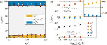
according to (2.32). The plot of the relative contributions to
 $\langle v_{n}\rangle$
in figure 10(a) shows that local entrainment at the selected thresholds is strongly dominated by viscous processes. The inviscid term associated with the vortex stretching mechanism contributes only approximately 6 %–8 % at the highest threshold and decreases to almost zero for the lowest value of
 $\unicode[STIX]{x1D714}_{th}^{2}$
. The ratio of the inviscid and viscous terms,
 $\unicode[STIX]{x1D716}\equiv \langle v_{n}^{{\mathcal{I}}}\rangle /[\langle v_{n}^{{\mathcal{I}}}\rangle +\langle v_{n}^{{\mathcal{D}}}\rangle +\langle v_{n}^{{\mathcal{E}}}\rangle ]$
, is between 2 % and 7 %, which locates the interfaces corresponding to the threshold levels chosen here inside or right at the border of the viscous superlayer, which van Reeuwijk & Holzner (Reference van Reeuwijk and Holzner2014) define based on the condition that
 $\unicode[STIX]{x1D716}<0.05$
. The blue shaded area in figure 10(a) represents the baroclinic torque, which constitutes a direct buoyancy effect on the relative motion of the enstrophy isosurface. The fraction of
 $\langle v_{n}^{{\mathcal{B}}}\rangle$
is approximately 12 % of
 $\langle v_{n}\rangle$
at the highest
 $\unicode[STIX]{x1D714}_{th}^{2}$
and decreases slightly down to approximately 8 % at the lowest threshold. It is also noteworthy that there is no discernible temporal dependence of the relative contributions in figure 10(a). Given the fact that these results are obtained using thresholds defined relative to the enstrophy level in the turbulent core, this also implies that the relative importance of the physical mechanisms responsible for the interface propagation behaves in a self-similar fashion. In other words, the physics of the local interface propagation is not dependent on the absolute but the relative enstrophy level.
Figure 10(b) displays the terms on the right-hand side of (2.32) normalized by
 $u_{n}$
. For the sake of clarity, the plot contains data at time
 $t/t^{\star }=150$
only, but the results are observed to be indifferent to
 $t$
. The dominant viscous contribution, whose net effect was considered in figure 10(a), is split up into
 $v_{n}^{{\mathcal{E}}}$
and
 $v_{n}^{{\mathcal{D}}}$
in figure 10(b). The term
 $v_{n}^{{\mathcal{E}}}$
is related to dissipation of enstrophy and is positive by definition, i.e. it causes the isosurface to move inward. It is, however, counteracted by viscous diffusion (
 $v_{n}^{D}$
), such that the net viscous effect is negative, resulting in an outward propagation of the interface. Dashed lines represent the prediction from a simple model for the interface propagation developed by van Reeuwijk & Holzner (Reference van Reeuwijk and Holzner2014), which was shown to be the exact solution in laminar flow (Philip et al.
Reference Philip, Bermejo-Moreno, Chung and Marusic2015). The main assumption of this model is that the interface is flat, an approximation that becomes increasingly valid the lower the threshold value is (cf. figure 9(c) and the related discussion). Consistently,
 $v_{n}^{{\mathcal{E}}}$
and
 $v_{n}^{{\mathcal{D}}}$
are closest to the respective model predictions of
 $-\langle v_{n}\rangle$
and
 $2\langle v_{n}\rangle$
at
 $\log _{10}(\unicode[STIX]{x1D714}_{th}^{2}/\hat{\unicode[STIX]{x1D714}}^{2})=-4.5$
. The inset of figure 10(b) indicates that
 $\langle v_{n}^{{\mathcal{I}}}\rangle /u_{\unicode[STIX]{x1D702}}$
decreases with smaller
 $\unicode[STIX]{x1D714}_{th}^{2}$
. In contrast, the dependence on
 $\unicode[STIX]{x1D714}_{th}^{2}$
is only weak for
 $\langle v_{n}^{{\mathcal{B}}}\rangle /u_{\unicode[STIX]{x1D702}}$
. The decrease of the relative buoyancy contribution at lower thresholds observed in figure 10(a) is therefore mostly due to the increase in
 $\langle v_{n}\rangle$
(which in turn is driven by an increase in the net viscous contribution). Hence, the threshold dependence of
 $v_{n}^{{\mathcal{B}}}$
is weaker than that of
 $v_{n}^{{\mathcal{I}}}$
.
(a) Relative decomposition of
 $\langle v_{n}\rangle$
into an inviscid part (bottom, shaded yellow), a net viscous contribution (centre, grey) combining the effects of viscous diffusion and dissipation, and a term directly related to the buoyancy field (top, blue). Shading and filled markers correspond to the highest threshold; open symbols indicate the decomposition at the lowest value of
 $\unicode[STIX]{x1D714}_{th}^{2}$
used. (b) Decomposition of
 $\langle v_{n}\rangle$
at
 $t/t^{\star }=150$
as a function of
 $\unicode[STIX]{x1D714}_{th}^{2}$
. The inset shows a blow-up focusing on the small contributions
 $v_{n}^{{\mathcal{I}}}$
and
 $v_{n}^{{\mathcal{B}}}$
. Results are shown for P4 only.

Finally, the p.d.f. of
 $v_{n}$
and its decomposition is plotted in figure 11 for a single time
 $t/t^{\star }=150$
and the highest threshold
 $\log _{10}(\unicode[STIX]{x1D714}_{th}^{2}/\hat{\unicode[STIX]{x1D714}}^{2})=-2.5$
. The results are nevertheless representative for other values of
 $t$
and
 $\unicode[STIX]{x1D714}_{th}^{2}$
. The distributions of
 $v_{n}^{{\mathcal{D}}}$
and
 $v_{n}^{{\mathcal{E}}}$
are much wider than the one of
 $v_{n}$
, indicative of the fact that large magnitudes of
 $v_{n}^{{\mathcal{D}}}$
are to at least some extent countered by large
 $v_{n}^{{\mathcal{E}}}$
. The p.d.f. of
 $v_{n}$
is still wide compared with its mean. Most importantly, it also covers positive values, which is evidence that locally also ‘detrainment’ events happen where previously turbulent fluid becomes non-turbulent. The figure further shows that
 $v_{n}^{{\mathcal{B}}}$
is not only comparatively small in the mean but also its variance (similar to that of
 $v_{n}^{{\mathcal{I}}}$
) is somewhat smaller than that of
 $v_{n}$
.
(a) Probability density function of
 $v_{n}$
and its decomposition according to (2.32) at
 $t/t^{\star }=150$
and
 $\log _{10}(\unicode[STIX]{x1D714}_{th}^{2}/\hat{\unicode[STIX]{x1D714}}^{2})=-2.5$
normalized by the Kolmogorov velocity
 $u_{\unicode[STIX]{x1D702}}$
. (b) The same plot with focus on small values of
 $v_{n}$
. Results are shown for P4 only.

Sketch of the ‘unstable’ (a) and ‘stable’ (b) configurations. The lines in (b) represent isodensity lines in the original state (dashed) and in a state distorted by the velocity profile (solid).

6 Discussion
The physical picture that emerges for the plume is that locally entrainment is a small-scale or ‘nibbling’ process, as advocated by Corrsin & Kistler (Reference Corrsin and Kistler1954). As our results show, buoyancy has a direct effect on this process. We find that the baroclinic torque supports the interface propagation with a contribution that is of similar, albeit not exactly the same, magnitude to the buoyancy contribution
 $(1-\unicode[STIX]{x1D703})Ri$
at the integral scale. The mechanism associated with positive
 $v_{n}^{{\mathcal{B}}}$
is sketched in figure 12(a). In the plume configuration (termed ‘unstable’ here), the mean buoyancy gradient is in the plane normal to the gravitational acceleration
 $\boldsymbol{g}$
. The spatially varying acceleration induced by this buoyancy distribution acts as a source of vorticity via the term
 $(\unicode[STIX]{x1D735}\times \boldsymbol{b})_{i}$
. In the mean, this vector is aligned with the vorticity vector of the mean shear such that the product
 $\unicode[STIX]{x1D714}_{i}(\unicode[STIX]{x1D735}\times \boldsymbol{b})_{i}$
that appears in (2.32) is positive. It is instructive to compare the present results with the case of an inclined gravity current, for which measurements of
 $v_{n}^{B}$
by Krug et al. (Reference Krug, Holzner, Lüthi, Wolf, Kinzelbach and Tsinober2015) exist. This flow configuration can be thought of as a plume that is deflected from the vertical by the presence of an inclined wall. As a consequence, alongside the unstable configuration discussed before, there exists a stable stratification between the core of the gravity current and the surrounding fluid, as sketched in figure 12(b). In this case,
 $\boldsymbol{g}$
and
 $\unicode[STIX]{x1D735}b$
are anti-aligned, and
 $(\unicode[STIX]{x1D735}\times \boldsymbol{b})_{i}$
acts as a restoring torque to deflections caused by
 $\unicode[STIX]{x1D714}_{i}$
; hence, the product of the two is negative. The experimental study by Krug et al. (Reference Krug, Holzner, Lüthi, Wolf, Kinzelbach and Tsinober2015) showed that even at an inclination angle as low as
 $10^{\circ }$
with respect to the horizontal, the unstable configuration dominates, resulting in a positive, even though small,
 $v_{n}^{{\mathcal{B}}}$
.
While the local propagation of the interface is a viscous process, the global entrainment rate is regulated by the surface area
 $A_{\unicode[STIX]{x1D702}}$
. The amplification by interface convolutions thereby acts in such a way that the overall entrainment rate is independent of viscosity, as suggested by, e.g., Townsend (Reference Townsend1976) and Tsinober (Reference Tsinober2009). In terms the long-standing debate on whether turbulent entrainment is due to small-scale ‘nibbling’ or large-scale ‘engulfment’ (cf. da Silva et al.
Reference da Silva, Hunt, Eames and Westerweel2014, and references therein), this view offers a Solomonic ruling: viscous nibbling is essential, but equally important are motions across the full range of scales, as they influence
 $A_{\unicode[STIX]{x1D702}}$
. In this sense, we advocate to replace the somewhat loosely defined concept of ‘engulfment’ by the more precise ‘amplification of viscous spreading due to interface convolutions’.
Whether or not there is a potential buoyancy effect on
 $A_{\unicode[STIX]{x1D702}}$
is hard to quantify from the present dataset due to the limited range of scales in the numerical data. The scaling relation
 $A_{\unicode[STIX]{x1D702}}/A_{0}\propto Re^{1/4}=(\unicode[STIX]{x1D702}/\hat{l})^{-1/3}$
is consistent with the power-law scaling
 $A_{\unicode[STIX]{x1D702}}/A_{0}\propto (\unicode[STIX]{x1D702}/\hat{l})^{2-D_{f}}$
with the fractal dimension
 $D_{f}=7/3$
(Sreenivasan et al.
Reference Sreenivasan, Ramshankar and Meneveau1989), which is commonly observed for the surface area of TNTIs in flows without buoyancy. Unlike in stably stratified flows (Mater & Venayagamoorthy Reference Mater and Venayagamoorthy2014), there is no cutoff of the scaling regime associated with buoyancy in the unstable configuration. It appears therefore plausible that the properties of
 $A_{\unicode[STIX]{x1D702}}$
remain unaltered when comparing, for example, a plume and a jet.
The question of why
 $\unicode[STIX]{x1D6FC}$
is found to be consistently higher in spatial plumes than in jets cannot be answered conclusively from the present results, not least because the situation appears to be reversed for temporal flows. A common hypothesis is to explain increased entrainment in spatial plumes by enhanced turbulence levels due to the effect of buoyancy (List Reference List1982; Kaminski et al.
Reference Kaminski, Tait and Carazzo2005; Carazzo et al.
Reference Carazzo, Kaminski and Tait2006). However, as van Reeuwijk & Craske (Reference van Reeuwijk and Craske2015) remark, this explanation appears questionable in view of the observation that
 $\unicode[STIX]{x1D6FF}$
is approximately equal in spatial jets and plumes. These doubts are corroborated by the latest DNS results of van Reeuwijk et al. (Reference van Reeuwijk, Salizzoni, Hunt and Craske2016), which show that the turbulence is actually very similar in spatial flows with and without buoyancy. This characteristic is apparently not present for temporal flows, where we find
 $\unicode[STIX]{x1D6FF}$
to be higher for jets than for plumes. Yet, the role of buoyancy is the same as in the spatial case, increasing the entrainment parameter in an integral as well as the local view. Based on these results, it appears that the positive contribution by the baroclinic torque to the spreading of turbulence might also be present in spatial flows and therefore offer a plausible explanation for enhanced entrainment in turbulent spatial plumes compared with spatial jets.
7 Summary and conclusion
In this paper, we have investigated buoyancy effects on the turbulent entrainment process in a global framework as well as locally using an interface-based approach, and have obtained consistent results. As part of the study, we introduced the concept of a temporally evolving plume as a simplified model for the spatial problem of pure plumes. We pointed out the analogy between temporal flows and jets and plumes in strong coflow and provided a comprehensive analysis of the new flow case along with a detailed description of how it can be implemented via DNS. Most notably, we found that the flow transitions to turbulence at
 $Re_{crit}\approx 420$
, and simulations should be halted once
 $\hat{l}/L_{y}\approx 0.3$
. Results regarding the entrainment analysis were based on two simulations that reached maximum Taylor–Reynolds numbers of
 $Re_{\unicode[STIX]{x1D706}}\approx 70$
and
 $Re_{\unicode[STIX]{x1D706}}\approx 100$
. Both plumes were observed to attain self-similar scaling with closely matching entrainment coefficients of
 $\unicode[STIX]{x1D6FC}_{0}=0.10$
. An integral analysis revealed that the absence of divergence of the streamwise transport in the temporal flow leads to a much simplified entrainment relation. Most of the missing terms are of the order of the ratio of transverse and streamwise length scales with respect to leading order in spatial flows and are neglected in the slender limit of the classical theory (Tennekes & Lumley Reference Tennekes and Lumley1994). However, the divergence of streamwise transport of mean energy is of leading order itself, and its absence in the temporal case constitutes a fundamental difference in the mean-flow behaviour. Consistent with findings for spatial flows, we found that at an integral level the bulk of the entrainment is associated with production of turbulent kinetic energy. An additional buoyancy contribution accounts for approximately 15 % of the total
 $\unicode[STIX]{x1D6FC}_{0}$
. Our analysis showed that, unlike in the spatial case where the streamwise transport factors in additionally, this buoyancy contribution is directly related to different shapes of the buoyancy and the velocity profiles in the temporal plume.
Further, we demonstrated that the entrainment coefficient can be obtained consistently by a local approach. In this framework, entrainment is defined as the local propagation of a TNTI relative to the fluid. We defined the TNTI via a threshold on enstrophy, and the results for the entrainment coefficient obtained from an interface-based analysis,
 $\unicode[STIX]{x1D6FC}_{l}$
, were observed to be largely threshold-independent over a range of threshold covering two orders of magnitude. Analogous to findings in flows without buoyancy, our results show that locally also in turbulent plumes the spreading of turbulence is predominantly due to viscous diffusion. However, our results indicate that this process is enhanced by an additional contribution due to the baroclinic torque, which is specific to flows featuring buoyancy. The baroclinic torque accounts for approximately 8 %–12 % of the mean local entrainment velocity
 $\langle v_{n}\rangle$
, with a slight tendency to decrease with increasing threshold values. This relative magnitude is comparable to the buoyancy effect at an integral level. Assuming that the small-scale processes near the TNTI do not differ between temporal and spatial plumes, the mechanism of enhanced small-scale spreading via the baroclinic torque offers a possible explanation for the fact that spatial plumes are commonly observed to entrain more than jets. Our finding that
 $v_{n}\sim u_{\unicode[STIX]{x1D702}}$
in plumes is in line with observations in other flow configurations (Holzner & Lüthi Reference Holzner and Lüthi2011; Wolf et al.
Reference Wolf, Lüthi, Holzner, Krug, Kinzelbach and Tsinober2012; Watanabe et al.
Reference Watanabe, Sakai, Nagata, Ito and Hayase2014; Krug et al.
Reference Krug, Holzner, Lüthi, Wolf, Kinzelbach and Tsinober2015). It implies that
 $v_{n}\propto Re^{-1/4}{\hat{w}}$
. It has further become apparent here that
 $A_{\unicode[STIX]{x1D702}}\propto t^{1/4}$
, which – using the fact that
 $Re\propto t$
for temporal plumes – leads to the Reynolds-number dependence
 $A_{\unicode[STIX]{x1D702}}\propto A_{0}Re^{1/4}$
. Hence, the total entrained volume flux given by the product
 $v_{n}A_{\unicode[STIX]{x1D702}}\propto A_{0}{\hat{w}}$
is independent of
 $Re$
, which lends support to the original entrainment hypothesis by Morton et al. (Reference Morton, Taylor and Turner1956), as stated in (1.1).
Acknowledgements
This work was supported by resources provided by The Pawsey Supercomputing Centre with funding from the Australian Government and the Government of Western Australia. The authors gratefully acknowledge support from the Australian Research Council and the University of Melbourne through the McKenzie fellowship.
Appendix A. Spatial plume in a coflow
We consider a high-
 $Re$
spatial plume in a uniform coflow
 $w_{\infty }$
, such that
 $\overline{w}_{s}=\overline{w}-w_{\infty }$
. In this case, the continuity equation is given by
 $$\begin{eqnarray}\frac{\unicode[STIX]{x2202}\overline{w}}{\unicode[STIX]{x2202}z}+\frac{\unicode[STIX]{x2202}\overline{v}}{\unicode[STIX]{x2202}y}=0\end{eqnarray}$$
and conservation of streamwise momentum reads
 $$\begin{eqnarray}\overline{v}\frac{\unicode[STIX]{x2202}\overline{w}}{\unicode[STIX]{x2202}y}+\overline{w}\frac{\unicode[STIX]{x2202}\overline{w}}{\unicode[STIX]{x2202}z}+\frac{\unicode[STIX]{x2202}}{\unicode[STIX]{x2202}y}\overline{v^{\prime }w^{\prime }}=\overline{b}.\end{eqnarray}$$
Using (A 1) and the fact that
 $w_{\infty }=\text{const}.$
, we arrive at
 $$\begin{eqnarray}\overline{v}\frac{\unicode[STIX]{x2202}\overline{w}_{s}}{\unicode[STIX]{x2202}y}+\overline{w}\frac{\unicode[STIX]{x2202}\overline{w_{s}}}{\unicode[STIX]{x2202}z}+\frac{\unicode[STIX]{x2202}}{\unicode[STIX]{x2202}y}\overline{v^{\prime }w^{\prime }}=\overline{b}.\end{eqnarray}$$
With the approximations
 $$\begin{eqnarray}\frac{\unicode[STIX]{x2202}}{\unicode[STIX]{x2202}z}\sim \frac{1}{L},\quad \frac{\unicode[STIX]{x2202}}{\unicode[STIX]{x2202}y}\sim \frac{1}{l},\quad \overline{w}\sim w_{\infty },\quad v^{\prime }\sim w^{\prime }\sim \overline{w}_{s}\sim w^{\ast },\end{eqnarray}$$
where
 $w^{\ast }$
and
 $b^{\ast }$
represent reference scales for the streamwise excess velocity and buoyancy respectively, we find from (A 1) that
 $\overline{v}\sim (l/L)w^{\ast }$
and for the terms in (A 3)
 $$\begin{eqnarray}\displaystyle & \left.\begin{array}{@{}l@{}}\displaystyle \overline{v}\frac{\unicode[STIX]{x2202}\overline{w}_{s}}{\unicode[STIX]{x2202}y}\sim \left(\frac{w^{\ast }}{w_{\infty }}\right)\frac{w_{\infty }w^{\ast }}{L},\\ \displaystyle \overline{w}\frac{\unicode[STIX]{x2202}\overline{w}_{s}}{\unicode[STIX]{x2202}z}\sim \frac{w_{\infty }w^{\ast }}{L},\\ \displaystyle \frac{\unicode[STIX]{x2202}}{\unicode[STIX]{x2202}y}\overline{v^{\prime }w^{\prime }}\sim \left(\frac{L}{l}\frac{w^{\ast }}{w_{\infty }}\right)\frac{w_{\infty }w^{\ast }}{L},\end{array}\right\} & \displaystyle\end{eqnarray}$$
 $$\begin{eqnarray}\displaystyle & \displaystyle \overline{b}\sim \frac{Lb^{\ast }}{w^{\ast }w_{\infty }}. & \displaystyle\end{eqnarray}$$
In the limit that
 $w^{\ast }\ll w_{\infty }$
and using the transformation
 $L=w_{\infty }t$
, the first term in (A 5) vanishes but the turbulent transport term is retained since
 $l/t\sim w^{\ast }$
. Consequently, (A 3) is transformed to
 $$\begin{eqnarray}\frac{\unicode[STIX]{x2202}\overline{w}_{s}}{\unicode[STIX]{x2202}t}+\frac{\unicode[STIX]{x2202}}{\unicode[STIX]{x2202}y}\overline{v^{\prime }w^{\prime }}=\overline{b}\end{eqnarray}$$
in the limiting case of strong coflow, which is equivalent to (2.4) in the inviscid case. Similarly, the scalar conservation equation in the presence of coflow is given by
 $$\begin{eqnarray}\overline{v}\frac{\unicode[STIX]{x2202}\overline{b}}{\unicode[STIX]{x2202}y}+\overline{w}\frac{\unicode[STIX]{x2202}\overline{b}}{\unicode[STIX]{x2202}z}+\frac{\unicode[STIX]{x2202}}{\unicode[STIX]{x2202}y}\overline{b^{\prime }v^{\prime }}=0,\end{eqnarray}$$
where, based on the estimates in (A 4), the individual terms are of order
 $$\begin{eqnarray}\displaystyle & \left.\begin{array}{@{}l@{}}\displaystyle \overline{v}\frac{\unicode[STIX]{x2202}\overline{b}}{\unicode[STIX]{x2202}y}\sim \left(\frac{w^{\ast }}{w_{\infty }}\right)\frac{w_{\infty }b^{\ast }}{L},\\ \displaystyle \overline{w}\frac{\unicode[STIX]{x2202}\overline{b}}{\unicode[STIX]{x2202}z}\sim \frac{w_{\infty }b^{\ast }}{L},\\ \displaystyle \frac{\unicode[STIX]{x2202}}{\unicode[STIX]{x2202}y}\overline{bv}\sim \left(\frac{L}{l}\frac{w^{\ast }}{w_{\infty }}\right)\frac{w_{\infty }b^{\ast }}{L}.\end{array}\right\} & \displaystyle\end{eqnarray}$$
Analogously, taking the limit
 $w^{\ast }\ll w_{\infty }$
and using the transformation
 $L=w_{\infty }t$
yields
 $$\begin{eqnarray}\frac{\unicode[STIX]{x2202}\overline{b}}{\unicode[STIX]{x2202}t}+\frac{\unicode[STIX]{x2202}}{\unicode[STIX]{x2202}y}\overline{b^{\prime }v^{\prime }}=0,\end{eqnarray}$$
which is again equivalent to the corresponding equations in the temporal plume case stated in (2.5). It is easy to see that the analogy between the temporal and coflow cases also holds for momentum-driven flows by setting
 $\overline{b}=0$
. We further note that for
 $0<w_{\infty }/w^{\ast }<\infty$
, there is a gradual transition from pure spatial to temporal development.
Appendix B. Integral analysis for a plane plume in the spatial case
Keeping the derivatives with respect to the streamwise direction when integrating (2.19)–(2.21) results in
 $$\begin{eqnarray}\displaystyle & \displaystyle \frac{\unicode[STIX]{x2202}}{\unicode[STIX]{x2202}t}B+\frac{\unicode[STIX]{x2202}}{\unicode[STIX]{x2202}z}\left(\unicode[STIX]{x1D703}\frac{MB}{Q}\right)=0, & \displaystyle\end{eqnarray}$$
 $$\begin{eqnarray}\displaystyle & \displaystyle \frac{\unicode[STIX]{x2202}}{\unicode[STIX]{x2202}t}Q+\frac{\unicode[STIX]{x2202}}{\unicode[STIX]{x2202}z}M=B, & \displaystyle\end{eqnarray}$$
 $$\begin{eqnarray}\displaystyle & \displaystyle \frac{\unicode[STIX]{x2202}}{\unicode[STIX]{x2202}t}M+\frac{\unicode[STIX]{x2202}}{\unicode[STIX]{x2202}z}\left(\unicode[STIX]{x1D6FE}\frac{M^{2}}{Q}\right)=2\unicode[STIX]{x1D703}\frac{MB}{Q}+2\unicode[STIX]{x1D6FF}\frac{M^{3}}{Q^{3}}, & \displaystyle\end{eqnarray}$$
instead of (2.22)–(2.24), with
 $\unicode[STIX]{x1D6FE}=Q/M^{2}\int _{-\infty }^{\infty }\overline{w}^{3}\,\text{d}y$
. The shape factor
 $\unicode[STIX]{x1D6FE}$
depends on the velocity profile only, and generally
 $\unicode[STIX]{x1D6FE}\geqslant 1$
(Craske & van Reeuwijk Reference Craske and van Reeuwijk2016). Specifically, the limiting case of
 $\unicode[STIX]{x1D6FE}=1$
relates to a top-hat distribution, and assuming a Gaussian shape we have for the 2D case
 $\unicode[STIX]{x1D6FE}=2\sqrt{3}/3\approx 1.15$
. From an evolution equation for the cross-section of the flow, the entrainment relation in the general case can be derived to be given by (Craske & van Reeuwijk Reference Craske and van Reeuwijk2015)
 $$\begin{eqnarray}\frac{1}{\unicode[STIX]{x1D6FE}}\frac{\unicode[STIX]{x2202}\hat{l}}{\unicode[STIX]{x2202}t}+\frac{\unicode[STIX]{x2202}Q}{\unicode[STIX]{x2202}z}=2\unicode[STIX]{x1D6FC}{\hat{w}},\end{eqnarray}$$
which leads to
 $$\begin{eqnarray}\unicode[STIX]{x1D6FC}=Ri\left(1-\unicode[STIX]{x1D703}\right)\frac{1}{\unicode[STIX]{x1D6FE}}-\frac{\unicode[STIX]{x1D6FF}}{\unicode[STIX]{x1D6FE}}+\left(1-\frac{1}{\unicode[STIX]{x1D6FE}}\right)\frac{Q^{2}}{M^{2}}\frac{\unicode[STIX]{x2202}M}{\unicode[STIX]{x2202}z}-\frac{\unicode[STIX]{x2202}}{\unicode[STIX]{x2202}z}\left(\ln \unicode[STIX]{x1D6FE}\right)\frac{Q^{2}}{2M}.\end{eqnarray}$$
Assuming stationary (
 $\unicode[STIX]{x2202}_{t}=0$
) and self-similar (
 $\unicode[STIX]{x2202}_{z}\unicode[STIX]{x1D6FE}=0$
) flow, (B 1) reduces to
 $\unicode[STIX]{x2202}_{z}M=B$
and we get
 $$\begin{eqnarray}\unicode[STIX]{x1D6FC}=\left(1-\frac{\unicode[STIX]{x1D703}}{\unicode[STIX]{x1D6FE}}\right)Ri-\frac{\unicode[STIX]{x1D6FF}}{\unicode[STIX]{x1D6FE}},\end{eqnarray}$$
which is the same result as the one obtained in van Reeuwijk & Craske (Reference van Reeuwijk and Craske2015) for round stationary self-similar plumes neglecting terms related to turbulence effects (cf. (3.6) in their paper). Comparing (B 6) with (2.27) again shows that the absence of mean streamwise energy transport is a fundamental difference in the temporal plume. We further note that (B 6) is consistent with the analysis for planar plumes carried out by Paillat & Kaminski (Reference Paillat and Kaminski2014), with differences in the formulation only resulting from their choice of using the buoyancy flux instead of
 $B$
.