2.1 Water structure

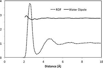
Water is a unique, small molecule with all three constituent atoms capable of forming hydrogen bonds. As a result, water molecules can cluster together in various arrangements, driven by their cooperative tendency to maximize the number of hydrogen bonds formed. Ab initio calculations suggest that a water hexamer (H₂O)₆ has several stable configurations of comparable energies that include cage, cyclic, chair, boat, and prismatic conformations (Moore Plummer & Chen, Reference Moore Plummer and Chen1987; Xantheas et al., Reference Xantheas, Burnham and Harrison2002; Xantheas & Dunning, Reference Xantheas and Dunning1994). Neutron and X-ray scattering have been used to characterize the average structure of bulk water. The radial distribution functions of OO, OH, and HH derived from these measurements provide valuable insight into local water structures (Root et al., Reference Root, Egelstaff and Hime1986; Soper, Reference Soper2000; Soper & Phillips, Reference Soper and Phillips1986; Sorenson et al., Reference Sorenson, Hura, Glaeser and Gordon2000). As an illustration, Fig. 1 shows the oxygen radial distribution function (RDF) around K⁺, denoting that the first peak of oxygen RDF around K⁺ is at an average separation of ∼2.8 Å between the closest water pair. The first peak extends to a minimum at ∼3.3 Å, indicating approximately 4.5 water molecules in the nearest coordination shell. The local structure of water has been rationalized as a ‘dynamic’ mixture of two states: one corresponds to a rigid ice-like structure, Ice I_h, a hexagonal crystal form of ordinary ice (Fletcher, Reference Fletcher1970) with four nearest neighbors at 2.8 Å; another corresponds to a denser ice-like structure, Ice II, a rhombohedral crystalline form with four water molecules at 2.8 Å plus another at 3.3 Å. Data from isochoric temperature differential experiments near the maximum-density-temperature peak, where the same densities can be achieved at two nearby temperatures, support the two-state theory (Bosio et al., Reference Bosio, Chen and Teixeira1983; Robinson et al., Reference Robinson, Cho and Urquidi1999; Sciortino et al., Reference Sciortino, Geiger and Stanley1990). Within this framework, properties such as the anomalous temperature dependence of the density can be interpreted as the dynamic competition between the two types of hydrogen-bonding networks in response to changes in temperature (Schmid et al., Reference Schmid, Michalsky, Slater, Barnard, Halthore, Liljegren, Holben, Eck, Livingston, Russell, Ingold and Slutsker2001).

Fig. 1.

Water structure and average dipole moment around a K⁺ ion. The radial distribution function (RDF) of O … K⁺ and water dipole moment were computed from molecular dynamic simulations of K⁺ in water using a polarizable potential (Grossfield et al., Reference Grossfield, Ren and Ponder2003; Ren & Ponder, Reference Ren and Ponder2003). Note that the average dipole moment of the water in the first solvation shell is roughly similar to that of bulk water.

2.2 Bulk water polarization

One of the fundamental properties of water is its role as an excellent solvent for polar molecules. Some aspects of this favorable polar molecular solvation can be understood from the very macroscopic continuum perspective of water bulk polarization. Water molecules have a dipole moment that varies between 1.8 Debye (D) in vacuum (Clough et al., Reference Clough, Beers, Klein and Rothman1973) to estimates of nearly 3 D in bulk water (Ren & Ponder, Reference Ren and Ponder2003; Silvestrelli & Parrinello, Reference Silvestrelli and Parrinello1999). In a liquid environment, the molecular dipole moment of water will reorient in response to the application of an external field or the introduction of a solute charge distribution. The resulting reorientation creates a polarization (or dipole) density or so-called ‘dielectric response’ (Bottcher, Reference Bottcher1952; Hansen & McDonald, Reference Hansen and Mcdonald2000; Jackson, Reference Jackson1975) (see Figs 1 and 2). From the perspective of continuum electrostatics, this dielectric behavior is modeled as a linear relationship between the local field and electric displacement field because of local polarization—the coefficient of this relationship is the ‘dielectric coefficient,’ or permittivity. Dielectric coefficients of pure solvent depend on a variety of molecular properties of the solvent, including structure, density, permanent charge distribution, and molecular polarizability. Dielectric coefficients range from values as small as 1 for a vacuum, to values of 2–4 for non-polar solvents (alkanes), 10–20 for weakly polar molecules such as ammonia and ethanol, to approximately 80 for water at room temperature, and even larger values for some polar liquids such as formamide (105).

Fig. 2.

The reorientation and polarization response of water upon the insertion of a cation (K⁺) into the bulk water. The yellow vector on each water molecule represents the net induced dipole moment because of the electric field of the ion and other water molecules. The white vector is the permanent (gas-phase) dipole moments (1.8 Debye) of the water molecule. The average dipole moment of a water molecule in liquid is 2.6–3.0 D according to various theoretical calculations. The snapshot is taken from molecular dynamics simulations of K⁺ in water using the AMOEBA potential (Ren & Ponder, Reference Ren and Ponder2003).

2.3 Electronic and nuclear water polarization

In addition to the bulk polarization of solvent, the charge distributions of solvent and solute molecules interact via mutual polarization, i.e., the reorganization of their electronic charge distributions. The reorganization of electrons is much faster than the overall reorientation and redistribution of solvent molecules (Nicol, Reference Nicol1974). It has been estimated that electronic solvation (as opposed to reorganization solvation) could account for as much as half of the overall electrostatic solvation free energy (Cukier & Zhang, Reference Cukier and Zhang1997). Processes such as photoexcitation and electron and proton transfers occur on timescales between or close to those of electronic and nuclear responses (Cramer & Truhlar, Reference Cramer, Truhlar, Rami Reddy and Erion2001). Theoretical frameworks have been devised to separate the solvent electronic and nuclear response either adiabatically or non-adiabatically (Marcus & Sutin, Reference Marcus and Sutin1985; Moser et al., Reference Moser, Keske, Warncke, Farid and Dutton1992). In theoretical studies, continuum or molecular mechanics (MM) solvent often supplements quantum mechanical treatment of the solutes (reactants).

2.4 Non-polar solvation by water

Another important aspect of solvation involves the mechanism of solvent interactions with uncharged solutes. This type of solvation phenomenon has many names including hydrophobic, apolar, and non-polar; we refer to it as non-polar solvation in this review. Non-polar solvation has been extensively studied and modeled, and there are many good references available for interested readers to explore, the following citations are only a few (Ben-Naim, Reference Ben-Naim2006; Hummer et al. Reference Hummer1999, Reference Hummer, Garde, Garcia and Pratt2000; Pratt, Reference Pratt2002; Pratt & Chandler Reference Pratt and Chandler1977, Reference Pratt and Chandler1980; Pratt & Pohorille, Reference Pratt and Pohorille2002). This section focuses on the basic properties of non-polar solvation important for the general aspects of biomolecule–solvent interactions.

Water's small size and flexibility in forming infinite hydrogen-bonding networks around solutes contribute to the hydrophobic effect that is widely appreciated in biology. Nuclear magnetic resonance (NMR) (Mizuno et al., Reference Mizuno, Oda, Maeda, Shindo and Okumura1995), high-performance liquid chromatography (HPLC) (Silveston & Kronberg, Reference Silveston and Kronberg1989), and neutron scattering (Soper, Reference Soper2000; Soper & Phillips, Reference Soper and Phillips1986) experiments suggested that water structure is different around a hydrophobic solute. Atomic and Monte Carlo simulations also support such structural change in water molecules, depending on surrounding environment (Lynden-Bell & Rasaiah, Reference Lynden-Bell and Rasaiah1997; Madan & Sharp, Reference Madan and Sharp1996). Efforts to understand hydration based on water structure and entropy changes date back several decades (Frank & Evans, Reference Frank and Evans1945). Sophisticated theories have been evolved to delineate the entropy and enthalpy contributions to solvation, the influence of dispersion and electrostatics, the effect of solute-length scale, temperatures, and other external factors to understand solvation phenomenon (Chandler, Reference Chandler2005; Garde et al., Reference Garde, Hummer, García, Paulaitis and Pratt1996; Hummer et al., Reference Hummer, Garde, Garcia and Pratt2000; Schmid et al., Reference Schmid, Michalsky, Slater, Barnard, Halthore, Liljegren, Holben, Eck, Livingston, Russell, Ingold and Slutsker2001). Advancements in molecular simulations have and will continue to help further our understanding of the role of solvation in biomolecular structure and dynamics.

Pioneering work by Pratt and Chandler (Pratt, Reference Pratt2002; Pratt & Chandler, Reference Pratt and Chandler1977, Reference Pratt and Chandler1980; Pratt & Pohorille, Reference Pratt and Pohorille1992, Reference Pratt and Pohorille2002) identified some of the fundamental determinants of non-polar solvation. Not surprisingly, a major contribution to the energetics of solvating an uncharged molecule is the energy required to create a cavity in the solvent. This cavity-creation term describes the work involved with accommodating within the solvent: purely strong solute–solvent repulsive interactions. Later work by Hummer et al. (Hummer et al., Reference Hummer, Garde, García, Pohorille and Pratt1996) translated this model in an information theory context by noting that the energetics of cavity creation are intrinsically encoded in the density fluctuations of the solvent. The energetics of cavity creation in water is strongly dependent on both the size and the shape of the non-polar solute with a crossover in energetics and solvent density near the solute interface when the solute size approaches nanometer-length scales (Ashbaugh, Reference Ashbaugh2009; Ashbaugh & Pratt, Reference Ashbaugh and Pratt2006; Ben-Amotz, Reference Ben-Amotz2005; Berne et al., Reference Berne, Weeks and Zhou2009; Choudhury & Pettitt, Reference Choudhury and Pettitt2007; Ewell et al., Reference Ewell, Gibb and Rick2008; Hummer & Garde, Reference Hummer and Garde1998; Li et al., Reference Li, Li, Eleftheriou and Zhou2006; Lum et al., Reference Lum, Chandler and Weeks1999; MacCallum et al., Reference Maccallum, Moghaddam, Chan and Tieleman2007; Rajamani et al., Reference Rajamani, Truskett and Garde2005). Another important aspect of non-polar solvation is the attractive nature between the solute and the solvent. For non-polar solvation, these attractive interactions are (by definition) not because of the electrostatics of static charge distributions on the solute and solvent, but are generally associated with weak dispersion interactions between solvent and solute originated from the fluctuation of induced dipoles within solvent and solute molecules (Boström & Ninham, Reference Boström and Ninham2005; Curutchet et al., Reference Curutchet, Orozco, Luque, Mennucci and Tomasi2006; Floris & Tomasi, Reference Floris and Tomasi1989; Floris et al., Reference Floris, Tomasi and Ahuir1991; Gallicchio et al., Reference Gallicchio, Kubo and Levy2000; Levy et al., Reference Levy, Zhang, Gallicchio and Felts2003; Pratt & Chandler, Reference Pratt and Chandler1980). If sufficiently weak, such attractive non-polar interactions are generally assumed not to affect the density of solvent around the solute, but instead simply change the energetics of solvation for a solvent density distribution determined by repulsive solvent–solute interactions. Note that non-polar solvation cannot be easily decoupled from the polar solvation process: strong attractive solute–solvent interactions can significantly affect local solvent densities and change the non-polar properties of the solvation process (Dzubiella & Hansen, Reference Dzubiella and Hansen2004; Dzubiella et al., Reference Dzubiella, Swanson and Mccammon2006a, Reference Dzubiella, Swanson and Mccammonb). Therefore, while the decomposition of solute–solvent interactions into polar and non-polar components is a useful conceptual device, the actual solvation process is much more complicated (Cramer & Truhlar, 1999, Reference Cramer and Truhlar2008).

Many biological phenomena are associated with non-polar solvation, ranging from protein folding to protein–protein to the fundamental structure and energetics of lipid bilayers and assemblies (Thirumalai & Hyeon, Reference Thirumalai and Hyeon2005; Yeagle, Reference Yeagle2004; Zhou et al., Reference Zhou, Huang, Margulis and Berne2004). A full discussion of the influence of non-polar solvation on the numerous aspects of biomolecular structure, function, and energetics would fill several reviews. Therefore, interested readers are referred to the excellent discussion of the topic provided by Pratt & Pohorille (Reference Pratt and Pohorille2002).

2.5 Site-specific binding and recognition

The discussion above has largely focused on the bulk properties of solvent and its non-specific interaction with solutes. However, a solvent such as water can also play a ligand-like role and interact with solutes in a decidedly non-bulk and site-specific manner. Perhaps the most familiar example of such site-bound solvent molecules are the crystallographic waters present at the surface (Kuhn et al., Reference Kuhn, Siani, Pique, Fisher, Getzoff and Tainer1992; Merzel & Smith, Reference Merzel and Smith2002; Smolin & Winter, Reference Smolin and Winter2004) and in cavities (Damjanović et al., Reference Damjanović, García-Moreno, Lattman and García2005a, Reference Damjanovic, Garciamorenoe, Lattman and GarciabReference Damjanović, Schlessman, Fitch, García and García-Moreno2007; Imai et al., Reference Imai, Hiraoka, Kovalenko and Hirata2005, Reference Imai, Hiraoka, Kovalenko and Hirata2007a) of many higher-resolution X-ray structures. While the physical and functional properties of such waters can be a subject of debate (Nayal & Di Cera, Reference Nayal and Di Cera1996), they are illustrative of the ways in which water can play structural as well as bulk roles in biomolecules. Nucleic acids provide another good illustration of how water can interact with biomolecular surfaces in a non-bulk-like and often sequence-specific manner (Arai et al., Reference Arai, Chatake, Ohhara, Kurihara, Tanaka, Suzuki, Fujimoto, Mizuno and Niimura2005; Auffinger & Hashem, Reference Auffinger and Hashem2007; Auffinger & Westhof, Reference Auffinger and Westhof2000a,b; Reference Auffinger and Westhof2001; Bastos et al., Reference Bastos, Castro, Mrevlishvili and Teixeira2004; Bonvin et al., Reference Bonvin, Sunnerhagen, Otting and Van Gunsteren1998; Fuxreiter et al., Reference Fuxreiter, Mezei, Simon and Osman2005; Mikulecky & Feig, Reference Mikulecky and Feig2006; Rhodes et al., Reference Rhodes, Réblová, Sponer and Walter2006; Yonetani et al., Reference Yonetani, Maruyama, Hirata and Kono2008), such as the zig-zag spine of hydration in the minor grove of B-DNA (Drew et al., Reference Drew, Samson and Dickerson1982). Structurally or specifically bound water can also play an important role in protein structure and function, including allosteric regulation (Bone, Reference Bone2006; Guinto & Di Cera, Reference Guinto and Di Cera1996; Krem & Di Cera, Reference Krem and Di Cera1998; Royer et al., Reference Royer, Pardanani, Gibson, Peterson and Friedman1996) and stability/flexibility (Fischer & Verma, Reference Fischer and Verma1999). Finally, water can play a very important role in molecular recognition; ranging from the binding of small molecules and peptides (Barillari et al., Reference Barillari, Taylor, Viner and Essex2007; Hamelberg & McCammon, Reference Hamelberg and Mccammon2004; Kuhn et al., Reference Kuhn, Siani, Pique, Fisher, Getzoff and Tainer1992; Petrone & Garcia, Reference Petrone and Garcia2004; Samsonov et al., Reference Samsonov, Teyra and Pisabarro2008; Thilagavathi & Mancera, Reference Thilagavathi and Mancera2010; van Dijk & Bonvin, Reference Van Dijk and Bonvin2006; Villacanas et al., Reference Villacanas, Madurga, Giralt and Belda2009), to protein–protein complexes (Ikura et al., Reference Ikura, Urakubo and Ito2004), to protein–nucleic acid binding (Billeter, Reference Billeter1996; Fried et al., Reference Fried, Stickle, Smirnakis, Adams, Macdonald and Lu2002; LiCata & Allewell, Reference Licata and Allewell1997), and water itself in the form of ice-binding and anti-freeze proteins (Doxey et al., Reference Doxey, Yaish, Griffith and Mcconkey2006; Jorov et al., Reference Jorov, Zhorov and Yang2004; Liu et al., Reference Liu, Jia, Chen, Tung and Liu2005; Yang & Sharp, Reference Yang and Sharp2004). Such specific characteristics of the solvent obviously need detailed molecular descriptions of the solvent, as described later in this review.

3.1 Non-specific screening

One of the simplest aspects of ionic behavior is the non-specific ‘mean field’ screening embodied in Debye–Hückel or Poisson–Boltzmann (PB) treatments of ionic solutions (Baker, Reference Baker2004; Gilson & Honig, Reference Gilson and Honig1988; Grochowski & Trylska, Reference Grochowski and Trylska2008; Lamm, Reference Lamm2003; Lamm & Pack, Reference Lamm and Pack2010). Such treatments assume ideal ion behavior where each ion experiences the average influence of its surrounding ionic environment. Therefore, this ‘mean field’ assumption implies no ion–ion correlations or fluctuations, effects that have been shown to be important in systems with high ion charge density (Angelini et al., Reference Angelini, Liang, Wriggers and Wong2003, Reference Angelini, Golestanian, Coridan, Butler, Beraud, Krisch, Sinn, Schweizer and Wong2006; Ben-Yaakov et al., Reference Ben-Yaakov, Andelman, Harries and Podgornik2009, Reference Ben-Yaakov, Andelman, Podgornik and Harries2011; Butler et al., Reference Butler, Angelini, Tang and Wong2003; Holm et al., Reference Holm, Kekicheff and Podgornik2001; Jho et al., Reference Jho, Kanduč, Naji, Podgornik, Kim and Pincus2008; Kanduč et al., Reference Kanduč, Trulsson, Naji, Burak, Forsman and Podgornik2008; Podgornik & Dobnikar, Reference Podgornik and Dobnikar2001; Todd et al., Reference Todd, Parsegian, Shirahata, Thomas and Rau2008; Todd & Rau, Reference Todd and Rau2008), as discussed later in this review. Additionally, these models assume no specific ion–ion, ion–solvent or ion–solute interactions; with a few exceptions (Baer & Mundy, Reference Baer and Mundy2011; Boström & Ninham, Reference Boström and Ninham2004; Boström et al., Reference Boström, Williams and Ninham2003a, Reference Boström, Williams, Stewart and Ninhamb; Jancovici, Reference Jancovici2006; Parsons et al., Reference Parsons, Boström, Nostro and Ninham2011), ions are typically treated as inert hard spheres with generic solute interactions based only on charge and steric repulsion. While the assumption of ideality makes such theories very convenient to implement and use, such assumptions are rarely valid in actual biomolecular systems (Anderson & Record, Reference Anderson and Record1995; Collins, Reference Collins1995; Marcus, Reference Marcus2006; Overman & Lohman, Reference Overman and Lohman1994; Record et al., Reference Record, Anderson and Lohman1978). Nevertheless, these models are very popular and have been successfully used to describe some aspects of ionic effects on biomolecular systems—particularly in highly dilute and low-charge density settings.

3.2 Site-specific binding

Unlike the non-specific aspects of ionic behavior discussed above, many ions interact with protein and nucleic acids in a site-specific manner. About one-third of all proteins contain metal ions as integral components (Chaturvedi & Shrivastava, Reference Chaturvedi and Shrivastava2005; Waldron & Robinson, Reference Waldron and Robinson2009). These metalloproteins—as well as other proteins that transiently bind ions—recognize and associate with only specific types of ions. This specificity allows them to discriminate and bind particular ion species, even in a solution of other ions of similar properties (e.g. charge and size). Specific interactions between ions and biomolecules can be critical for maintaining structure and are often directly involved in function as well. There are several examples where specific ion binding plays a key role in biomolecular structure. These include RNA tertiary structure stability (Adams et al., Reference Adams, Stahley, Kosek, Wang and Strobel2004; Auffinger & Hashem, Reference Auffinger and Hashem2007; Cate et al., Reference Cate, Gooding, Podell, Zhou, Golden, Kundrot, Cech and Doudna1996; Conn et al., Reference Conn, Gittis, Lattman, Misra and Draper2002; Draper, Reference Draper2008; Draper et al., Reference Draper, Grilley and Soto2005; Grilley et al., Reference Grilley, Misra, Caliskan and Draper2006, Reference Grilley, Soto and Draper2007; Leipply & Draper, Reference Leipply and Draper2000) as well as several protein assembly and stability examples (Calimet & Simonson, Reference Calimet and Simonson2006; Ding & Dokholyan, Reference Ding and Dokholyan2008; Li et al., Reference Li, Zhang, Wang and Wang2008; Wong & Pollack, Reference Wong and Pollack2010). Additionally, the functions of many proteins are affected by specific ion binding. For example, thrombin, a key enzyme in blood coagulation, is allosterically activated by Na⁺ (Guinto & Di Cera, Reference Guinto and Di Cera1996; Wells & Di Cera, Reference Wells and Di Cera1992); the NikR DNA-binding protein is activated by Ni²⁺ binding (Benanti & Chivers, Reference Benanti and Chivers2007; Bradley et al., Reference Bradley, Chivers and Baker2008; Carrington et al., Reference Carrington, Chivers, Al-Mjeni, Sauer and Maroney2003; Chivers & Sauer, Reference Chivers and Sauer2000); and calmodulin undergoes significant conformational transitions in response to calcium binding (Bertini et al., Reference Bertini, Del Bianco, Gelis, Katsaros, Luchinat, Parigi, Peana, Provenzani and Zoroddu2004; Evans et al., Reference Evans, Hell and Shea2011; Mori et al., Reference Mori, Erickson and Yue2004). Many other systems are also regulated by ion binding (Benanti & Chivers, Reference Benanti and Chivers2007; Carrington et al. Reference Carrington, Chivers, Al-Mjeni, Sauer and Maroney2003; Chivers & Sauer, Reference Chivers and Sauer2000; Gohara & Di Cera Reference Gohara and Di Cera2011; Hedstrom et al. Reference Hedstrom, Szilagyi and Rutter1992; Niu et al. Reference Niu, Chen, Bush-Pelc, Bah, Gandhi and Di Cera2009; Page et al. Reference Page, Bleackley, Wong, Macgillivray and Di Cera2006; Reyes-Caballero et al. Reference Reyes-Caballero, Campanello and Giedroc2011; Shults et al. Reference Shults, Pearce and Imperiali2003).

The definition of site-specific binding can be broadened somewhat to also include the specific recognition and binding of particular ions to more generic structural features of nucleic acids (Auffinger & Hashem, Reference Auffinger and Hashem2007) and lipid bilayers. For example, different species of ions are known to compete for binding to the DNA minor groove, leading to a preferential accumulation of particular cation species in this region of DNA molecules (Auffinger & Westhof, Reference Auffinger and Westhof2001; Marincola et al., Reference Marincola, Denisov and Halle2004; Savelyev & Papoian, Reference Savelyev and Papoian2006; Tikhomirova & Chalikian, Reference Tikhomirova and Chalikian2004). Such specificity is also observed around other nucleic acid structures, including RNA (Chen & Honig, Reference Chen and Honig1997; Chen et al., Reference Chen, Draper and Pappu2009a, Reference Chen, Marucho, Baker and Pappub; García-García & Draper, Reference García-García and Draper2003; Grilley et al., Reference Grilley, Misra, Caliskan and Draper2007; Misra & Draper, Reference Misra and Draper1999, Reference Misra and Draper2000, Reference Misra and Draper2001, Reference Misra and Draper2002; Misra et al., Reference Misra, Shiman and Draper2003; Savelyev & Papoian, Reference Savelyev and Papoian2006; Soto et al., Reference Soto, Misra and Draper2007). Ion specificity for particular regions of nucleic acid and protein structure can also manifest itself in effects on protein-DNA recognition (Kozlov & Lohman, Reference Kozlov and Lohman1998; Mauro & Koudelka, Reference Mauro and Koudelka2004; Overman & Lohman, Reference Overman and Lohman1994; Record et al., Reference Record, Anderson and Lohman1978), although such effects can often arise from a wide range of interaction types (Overman & Lohman, Reference Overman and Lohman1994; Record et al., Reference Record, Anderson and Lohman1978, Reference Record, Olmsted, Bond, Anderson and Record1995; Zhang et al., Reference Zhang, Ni, Capp, Anderson, Lohman and Record1999). In a similar manner, the differential interface-perturbing behavior of monovalent cations on membrane surface properties and membrane curvature is associated with their different hydration tendencies that will modulate the extent and stability of the hydrogen-bond network along the charged membrane surface (Kraayenhof, Reference Kraayenhof1996).

3.3 Ion–water interactions

Many species-specific ion effects are governed, in part, by ion–water interactions. Studies of such preferential hydration are far too numerous to include in a single review; indeed, many excellent manuscripts and texts have been written on the basic physical chemistry of these interactions (Kielland, Reference Kielland1937; Nightingale, Reference Nightingale1959; Robinson & Stokes, Reference Robinson and Stokes2002) as well as their biophysical implications (Courtenay et al., Reference Courtenay, Capp and Record2001; Record et al., Reference Record, Anderson and Lohman1978, Reference Record, Olmsted, Bond, Anderson and Record1995; Timasheff, Reference Timasheff1998, Reference Timasheff2002). Ions are known to significantly perturb the structure of water (Ansell et al., Reference Ansell, Barnes, Mason, Neilson and Ramos2006; Hribar et al., Reference Hribar, Southall, Vlachy and Dill2002; Zangi et al., Reference Zangi, Hagen and Berne2007) and the strength of their interaction with water can significantly influence their affinity for interfaces (Collins, Reference Collins1995; Pegram & Record, Reference Pegram and Record2006, Reference Pegram and Record2007). One of the most famous observations of this behavior is the Hofmeister effect (Baldwin, Reference Baldwin1996; Hofmeister, Reference Hofmeister1888), which ranks ions based on their ability to precipitate or destabilize protein structures (Baldwin, Reference Baldwin1996; Collins, Reference Collins1995; Timasheff, Reference Timasheff1992), or partition to aqueous interfaces (Chen et al., Reference Chen, Yang, Kataoka and Cremer2007b; Pegram & Record, Reference Pegram and Record2006, Reference Pegram and Record2007, Reference Pegram and Record2008). Hofmeister-like behavior also correlates with specific tendencies to enter the Stern layer and to bind the surface for charge neutralization. Roughly speaking, the Hofmeister effect can be described as a rank of ions (given valence) to adsorb in directly proportional to their unhydrated size. Hofmeister effects are particularly prevalent when local ion concentrations are high and play a role in a wide range of biological processes, including protein folding (Baldwin, Reference Baldwin1996; Timasheff, Reference Timasheff1992), protein–DNA interactions (Hong et al., Reference Hong, Capp, Anderson, Saecker, Felitsky, Anderson and Record2004; Kozlov & Lohman, Reference Kozlov and Lohman1998; Shimizu, Reference Shimizu2004a, Reference Shimizub; Shimizu & Smith, Reference Shimizu and Smith2004; Shimizu et al., Reference Shimizu, Mclaren and Matubayasi2006; Timasheff, Reference Timasheff2002), nucleic acid stability (Pegram et al., Reference Pegram, Wendorff, Erdmann, Shkel, Bellissimo, Felitsky and Record2010; Pincus et al., Reference Pincus, Hyeon and Thirumalai2008), and biomembrane behavior (Aroti et al., Reference Aroti, Leontidis, Maltseva and Brezesinski2004, Reference Aroti, Leontidis, Dubois and Zemb2007; Boström & Ninham, Reference Boström and Ninham2005; Boström et al., Reference Boström, Williams, Stewart and Ninham2003b; Clarke & Lüpfert, Reference Clarke and Lüpfert1999; Fukuma et al., Reference Fukuma, Higgins and Jarvis2007; Leontidis et al., Reference Leontidis, Aroti, Belloni, Dubois and Zemb2007; Sachs & Woolf, Reference Sachs and Woolf2003; Vácha et al., Reference Vácha, Siu, Petrov, Böckmann, Barucha-Kraszewska, Jurkiewicz, Hof, Berkowitz and Jungwirth2009). While there are a number of theories for the detailed physical basis of the Hofmeister effect (Baldwin, Reference Baldwin1996; Boström & Ninham, Reference Boström and Ninham2004; Boström et al., Reference Boström, Williams and Ninham2003a, Reference Boström, Williams, Stewart and Ninhamb; Parsegian et al., Reference Parsegian, Rand and Rau2000; Parsons et al., Reference Parsons, Boström, Maceina, Salis and Ninham2010, Reference Parsons, Boström, Nostro and Ninham2011; Pegram & Record, Reference Pegram and Record2008; Shimizu et al., Reference Shimizu, Mclaren and Matubayasi2006; Tang & Bloomfield, Reference Tang and Bloomfield2002; Zhou, Reference Zhou2005), there is not yet broad consensus on the best way to model this phenomenon in computational treatments of biomolecular electrostatics. Perhaps the most straightforward model currently available uses dispersion effects to reproduce Hofmeister trends in continuum models of ion behavior (Boström & Ninham, Reference Boström and Ninham2004; Boström et al., Reference Boström, Williams and Ninham2003a, Reference Boström, Williams, Stewart and Ninhamb, Reference Boström and Ninham2005; Parsons et al., Reference Parsons, Boström, Nostro and Ninham2011). While dispersion forces have been implicated in Hofmeister-like behavior (Boström & Ninham, Reference Boström and Ninham2004, Reference Boström and Ninham2005; Boström et al. Reference Boström, Williams and Ninham2003a, Reference Boström, Williams, Stewart and Ninhamb, Reference Boström, Kunz and Ninham2005a, Reference Boström, Tavares, Bratko and Ninhamb; Gurau et al., Reference Gurau, Lim, Castellana, Albertorio, Kataoka and Cremer2004; Ninham & Yaminsky, Reference Ninham and Yaminsky1997; Parsons et al., Reference Parsons, Boström, Maceina, Salis and Ninham2010, Reference Parsons, Boström, Nostro and Ninham2011), they are unlikely to be the only contributing interaction (Lund et al., Reference Lund, Jungwirth and Woodward2008a, Reference Lund, Vacha and Jungwirthb; Shimizu et al., Reference Shimizu, Mclaren and Matubayasi2006; Tobias & Hemminger, Reference Tobias and Hemminger2008). Therefore, it is unlikely that any current continuum solvation model completely describes these types of preferential solvation and Hofmeister effects.

4.1 Electric moments and Coulombic interactions

The importance of Coulombic interactions in molecular energies and forces has been recognized for a long time. Feynman discussed the importance of such interactions in 1939 (Feynman, Reference Feynman1939) while Buckingham (Buckingham, Reference Buckingham1967) began his 1967 seminal paper with the statement, ‘There is now general agreement that the significant forces between atoms and molecules have an electric origin.’ Quantum mechanical forces that act among molecules are electrostatic in nature. For example, repulsion results from electron overlap when atoms approach each other without forming chemical bonds; dispersive attraction can arise from interactions from instantaneous fluctuation of charge distribution inside molecules. In classical mechanics, the non-covalent interatomic interactions are partitioned into electrostatics as described by Coulomb's law, van der Waals exchange-repulsion and dispersion, as well as secondary contributions such as induction and charge transfer (Stone, Reference Stone1996). Although all major contributions need to be represented effectively in modeling molecular interactions, a consistent and transferable treatment of electrostatic interaction has been particularly challenging. The key issues include representation of charge distribution, efficient and accurate description of long-range interactions, and solvent effects.

The first molecular dynamics simulation of water was reported by Rahman and Stillinger in 1971 (Rahman, Reference Rahman1971). Four artificial point charges (±0.19e) were placed 1 Å away from the oxygen atom to model the electrostatic interaction between water molecules. The use of effective point charges to represent the charge distribution of atoms and molecules greatly reduces the computational needs to study large molecules and condensed matters in comparison with quantum mechanical methods where electrons are considered in detail. The application of QM-derived point charges to investigate molecular systems dates back at least to the mid-1960s (Bradley et al., Reference Bradley, Lifson and Honig1964; Kimel, Reference Kimel1964; Lifson, Reference Lifson1968) with several important later contributions (Allinger, Reference Allinger, Gold and Bethell1976). The electrostatic interaction is commonly modeled via partial charges located at atomic centers; for example, in the following force fields: AMBER (assisted model building with energy refinement) (Case et al., Reference Case, Cheatham, Darden, Gohlke, Luo, Merz, Onufriev, Simmerling, Wang and Woods2005; Cornell et al., Reference Cornell, Cieplak, Bayly, Gould, Merz, Ferguson, Spellmeyer, Fox, Caldwell and Kollman1995), MMFF (Merck molecular force field), OPLS (optimized potentials for liquid simulations) (Kaminski et al., Reference Kaminski, Friesner, Rives and Jorgensen2001), CHARMM (Chemistry at HARvard Macromolecular Mechanics) (MacKerell et al., Reference Mackerell, Bashford, Dunbrack, Evanseck, Field, Fischer, Gao, Guo, Ha, Joseph-Mccarthy, Kuchnir, Kuczera, Lau, Mattos, Michnick, Ngo, Nguyen, Prodhom, Reiher, Roux, Schlenkrich, Smith, Stote, Straub, Watanabe, Wiórkiewicz-Kuczera, Yin and Karplus1998).

The electrostatic potential (ESP) energy U for a system of point charges follows Coulomb's law:

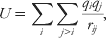(1)$$U \equals \sum\limits_{i} {\sum\limits_{j \gt i} {{{q_{i} q_{j} } \over {r_{ij} }}} } \comma $$

where q denotes the charge value and r is the distance between charge locations. The ESP from atomic partial charges can be systematically improved by using a multipole expansion to describe the charge distribution (Buckingham, Reference Buckingham1967). For an arbitrary charge distribution (e.g. an atom or a molecule) described by charges q _i (i = 1, …, n), the ESP at a distance R away from the particle is given by the sum:

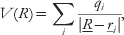(2)$$V\lpar R\rpar \equals \sum\limits_{i} {{{q_{i} } \over {\left\vert {\underline R \minus \underline r _{i} } \right\vert}}} \comma $$

where the | | notation refers to Euclidean distance. For a distance R>r, a Cartesian–Taylor expansion of the above equation leads to

(3)$$V\lpar R\rpar \equals \left\{ {\sum\limits_{i} {q_{i} } \minus \underline \mu \cdot \nabla \plus {1 \over 2}\underline{\underline \rmTheta } \colon \nabla ^{\setnum{2}} \minus \cdots } \right\}\left( {{1 \over R}} \right)$$

a multipole representation where the symbol ∇ denotes the gradient operator. The first term inside the bracket is the sum of charges of the particle or monopole moment. The dipole moment of the charge distribution μ is a vector with three components: $\mu _{\alpha } \equals < $> <$> \sum\nolimits_{i} {q_{i} r_{i\alpha } } {\rm \comma }\;{\rm where} \ \alpha \equals x\comma \, y\comma \, z$. The quadrupole moment tensor ($\underline{\underline \rmTheta } $) has nine components given by $\rmTheta _{}^{\alpha \beta } \equals \sum\nolimits_{i} {q_{i} r_{i\alpha } r_{i\beta } } $. A traceless form of the quadrupole tensor $\rmTheta _{}^{\alpha \beta } \equals <$> <$ > \sum\nolimits_{i} {q_{i} \lpar {\textstyle{3 \over 2}}r_{i\alpha } r_{i\beta } \minus {\textstyle{1 \over 2}}r_{i} ^{\setnum{2}} \delta _{\alpha \beta } \rpar } $, instead of the traced one, can be used in Equation (3), along with constant 1/2 before $\underline{\underline \rmTheta } \colon \nabla ^{\setnum{2}} $ replaced by 1/3 (Stone, Reference Stone1996). A spherical form of multipole expansion can also be obtained by a spherical harmonic expansion (Bottcher, Reference Bottcher1952; Hirschfelder et al., Reference Hirschfelder, Curtiss and Bird1954; Kirkwood, Reference Kirkwood1934; Stone, Reference Stone1996).

Molecular multipole moments can be more efficient than point charges for modeling molecular electrostatic interactions, even though the associated energy and derivatives are more complex. In fact, early simulations of liquid and solid benzene adopted potentials that included a point quadrupole at the center of the benzene molecule (Claessens et al., Reference Claessens, Ferrario and Ryckaert1983; Jorgensen & Swenson, Reference Jorgensen and Swenson1985; Linse, Reference Linse1984). It was suggested (Claessens et al., Reference Claessens, Ferrario and Ryckaert1983) that the potential with a point multipole was superior to the Lennard–Jones-only potential for crystal structure prediction even though a recent study indicated that electrostatic interactions are not critical in predicting crystal packing of non-polar molecules (Della Valle et al., Reference Della Valle, Venuti, Brillante and Girlando2008). Because of the assumption of R>r in the Taylor expansion in Equation (3), however, the molecular multipole expansion is problematic at the short distances that are often relevant in molecular simulation. The multipole expansion may diverge within the sphere R, and lead to an inaccurate ESP. The solution to overcome this issue is to distribute the multipole expansion to a collection of sites within the molecule, which effectively reduces the radius of the divergence sphere (Fowler & Buckingham, Reference Fowler and Buckingham1983, Reference Fowler and Buckingham1991; Price, Reference Price1985; Stone, Reference Stone1981).

Buckingham and Fowler (Fowler & Buckingham, Reference Fowler and Buckingham1983) were the first to apply distributed multipoles to the study of small molecule complexes. Atomic multipoles can be derived in several ways, including the distributed multipole analysis (DMA) of an ab initio wavefunction (Stone, Reference Stone1981). The combination of a hard sphere potential with atomic multipoles (up to quadrupole) was rather successful in reproducing experimental geometries including hydrogen-bonding distance and angle for several molecular complexes. It has been noted that local atomic charge distributions are usually not spherically symmetrical because of chemical bonding and lone pairs, and thus higher-order electrostatic moments are necessary to describe such features. Systematic study of the accuracy of point multipole models also has been described (Williams, Reference Williams1988). It was shown that the use of higher-order multipole moments significantly improved the representation of molecular ESP in comparison with ab initio reference potential. When only atomic charges were allowed, the relative root-mean-squared error in the ESP around the molecules was of the order of 10%. With the addition of dipole and quadrupole moments, the error was reduced by orders of magnitude to less than 0.1% (Williams, Reference Williams1988). Considering that higher-order moments decay faster than monopoles, the advantage of a distributed multipole expansion is to improve the short-range description outside the van der Waals surface of a molecule, which is important for interactions such as hydrogen bonding (Dykstra, Reference Dykstra1993).

An alternative to multipole expansion is to use a number of charge sites, which should in principle, offer a similar improvement to the accuracy of the molecular ESP. A great advantage of using point charges is the simplicity of the energy and atomic gradient; in contrast, the gradient and torque on point multipoles require significantly more algebra. There have been arguments that a point charge model is more efficient for a given level of accuracy, at least for diatomic molecules such as HF and HCl (Brobjer & Murrell, Reference Brobjer and Murrell1982). There are also models that replace multipole moments by distributed point charges (Sokalski et al., Reference Sokalski, Keller, Ornstein and Rein1993). The extended electron distribution (XED) force field adopts an explicit charge distribution around each atom, which seems to give improvements in interaction energy, conformation, and electrostatic field (Chessari et al., Reference Chessari, Hunter, Low, Packer, Vinter and Zonta2002; Vinter, Reference Vinter1996). Some versions of the AMBER force field place charges at important lone-pair sites (Dixon & Kollman, Reference Dixon and Kollman1997). Another recent example is the TIP5P water model, which employs five charge sites. However, it was shown that the determination of the exact locations of the lone pair charges was not trivial, and involved an extensive fitting procedure to reproduce experimental density-temperature profiles (Mahoney & Jorgensen, Reference Mahoney and Jorgensen2000; Rick, Reference Rick2001). Another concern is that charges located away from atomic centers may lead to numerical instability in molecular dynamics or Monte Carlo simulations because of the potential fusion of charge sites.

To evaluate the interaction between multipole moments, Applequist introduced a concise polytensor scheme (Applequist, Reference Applequist1983, Reference Applequist1984, Reference Applequist1985, Reference Applequist1989; Dykstra, Reference Dykstra1988). The multipole expansion at site k is written as

(4)$$M_{i} \equals \left[ {q_{i} \comma \ \mu _{ix} \comma \ \mu _{ix} \mu _{ix} \comma \rmTheta _{ixx} \comma \rmTheta _{ixy} \comma \ldots } \right]^{t} \comma $$

where the superscript t indicates transpose. The interaction energy between two multipoles at sites i and j is then given by the matrix formula:

$$U_{ij} \equals M_{i}^{t} T_{ij} M_{j} \comma $$

where T is the interaction matrix:

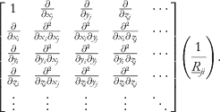$$\left[ {\matrix{ 1 \tab {{\partial \over {\partial x_{j} }}} \tab {{\partial \over {\partial y_{j} }}} \tab {{\partial \over {\partial z_{j} }}} \tab \cdots \cr {{\partial \over {\partial x_{i} }}} \tab {{{\partial ^{\setnum{2}} } \over {\partial x_{i} \partial x_{j} }}} \tab {{{\partial ^{\setnum{2}} } \over {\partial x_{i} \partial y_{j} }}} \tab {{{\partial ^{\setnum{2}} } \over {\partial x_{i} \partial z_{j} }}} \tab \cdots \cr {{\partial \over {\partial y_{i} }}} \tab {{{\partial ^{\setnum{2}} } \over {\partial y_{i} \partial x_{j} }}} \tab {{{\partial ^{\setnum{2}} } \over {\partial y_{i} \partial y_{j} }}} \tab {{{\partial ^{\setnum{2}} } \over {\partial y_{i} \partial z_{j} }}} \tab \cdots \cr {{\partial \over {\partial z_{i} }}} \tab {{{\partial ^{\setnum{2}} } \over {\partial z_{i} \partial x_{j} }}} \tab {{{\partial ^{\setnum{2}} } \over {\partial z_{i} \partial y_{j} }}} \tab {{{\partial ^{\setnum{2}} } \over {\partial z_{i} \partial z_{j} }}} \tab \cdots \cr \vdots \tab \vdots \tab \vdots \tab \vdots \tab \ddots \cr} } \right]\left( {{1 \over {\underline R _{ji} }}} \right).$$

The multipole moments here are defined in the same global frame. For example, Price reported distributed multipoles for amides and peptides in predefined molecular axes (Faerman & Price, Reference Faerman and Price1990). Alternatively, it is possible to define the multipole moments for each atom type in a local coordinate frame that is constructed with respect to covalently bonded neighboring atoms. Within this scheme, the oxygen atom in the water molecule may use the so-called bisector frame where the z-axis is the bisector of the HOH angle (Kong, Reference Kong1997; Ren & Ponder, Reference Ren and Ponder2003); the x-axis is perpendicular to z and also lies in the HOH plane; and the y-axis is determined via the right-hand rule. For chemical systems without such symmetry, a generic z-then-x local frame can be used, in which one chemical bond to a neighboring atom is selected to define the z-axis.

A rotation matrix converts local multipole moments into the global frame prior to computation of the electrostatic interaction energies. Many algorithms require the evaluation of the analytic electrostatic forces for each molecular configuration. For the atomic charge model, the force is simply the negative derivative of Coulomb energy (1/r) with respect to atomic coordinates. For an atomic multipole expansion, forces are derived in a similar fashion by taking the derivative of the interaction matrix T and, using the relationships $T^{\lpar n \plus \setnum{1}\rpar } \equals \nabla \lpar T^{n} \rpar $, and $T^{\setnum{0}} \equals {\raise0.5ex\hbox{$\scriptstyle 1$}\kern-0.1em/\kern-0.15em\lower0.25ex\hbox{$\scriptstyle R$}}$. Expressions for the first few derivatives are available (Kong, Reference Kong1997). A further complication must be considered for dipole and higher-order moments. From a physics point of view, a dipole moment placed in an external field will experience a torque that favors rotation of the site (and its local frame defining neighbors). It is possible to convert each torque into forces at frame-defining sites to permit standard molecular dynamics integration schemes or optimization algorithms (Ren & Ponder, Reference Ren and Ponder2003). There is an alternative approach to understand these extra forces mathematically. If the multipole moments defined within their local frames are explicitly included in the energy expression with their rotation matrix, which is a function of atomic coordinates, the product rule leads to these additional forces (Kong, Reference Kong1997). Besides the Cartesian poly-tensor approach explained above, the spherical tensor formulations of the multipole interaction energy, force, and torque, are available (Price et al., Reference Price, Stone and Alderton1984).

Note that even with the better convergence of atomic multipole at short range, there are errors associated with the point approximation of the charge distribution. At a distance where electron density is penetrated, a negative (attractive) penetration effect is missing from the point multipole potential energy (Stone, Reference Stone1996). It has been suggested that the penetration effect could be absorbed by the repulsive term or possibly by damping the Coulomb energy (Klopper et al., Reference Klopper, Van Duijneveldt-Van De Rijdt and Van Duijneveldt2000; van Duijnen & Swart, Reference Van Duijnen and Swart1998). Wheatley & Mitchell (Reference Wheatley and Mitchell1994) proposed replacing the point multipole with Gaussian multipoles to correctly model the penetration effect at short range. Piquemal et al. (Reference Piquemal, Williams-Hubbard, Fey, Deeth, Gresh and Giessner-Prettre2003) used s-type Gaussian functions distributed at multi-sites to represent the charge density. In the recent development of Quantum Mechanics Polarizable Force Field (QMPFF) (Donchev, Reference Donchev2006; Donchev et al., Reference Donchev, Ozrin, Subbotin, Tarasov and Tarasov2005), a model was developed that consists of a nuclear charge and a negative electron cloud of exponential form located off the nuclear center. These more sophisticated treatments are likely to provide greater flexibility and higher accuracy for modeling electrostatics, within the limits of the ab initio data to which they are fit, although at higher computational cost.

When formulating an MM potential, conventional wisdom is that intramolecular short-range electrostatic interactions should be masked (scaled), based on the rationale that bond and angle energy terms already include these interactions. However, details of the masking schemes vary among different force fields. For example, charge interactions between the 1–2 (directly bonded) and the 1–3 (separated by two bonds) atoms are almost universally omitted. The 1–4 (atoms separated by three bonds) interaction is scaled down by 5/6 in Amber94, by 1/2 in OPLS-AA, and is not modified in CHARMM. These scaling factors are determined empirically to best reproduce conformational energy profile of flexible molecules.

Parameterization of realistic charge distributions, in the forms of point charges or higher-order moments, is essential to the accuracy of electrostatic energetics. Although atomic charges are not measurable physical quantities (physical observables), it is possible to derive meaningful values from quantum mechanical calculations. A method such as Mulliken population analysis or Bader's Atoms-in-Molecules (AIM) theory partitions electron density into atomic contributions (Bader, Reference Bader1990). However, different partitioning schemes lead to substantially different atomic charges. Momany first treated atom charges as adjustable parameters and derived values by fitting to ab initio Electrostatic potential (ESP) (Momany, Reference Momany1978). Unlike atomic charges, ESPs are physical observables and are directly associated with intermolecular interactions. Cox & Williams (Reference Cox and Williams1981) pointed out that ESPs from Mulliken charges generally had significant errors. Variants of ESP fitting approaches include CHarges from Electrostatic Potentials (CHELP), CHarges from Electrostatic Potentials using a Grid based method (CHELPG) (Breneman & Wiberg, Reference Breneman and Wiberg1990), Merz-Kollman (MK), and Restrained Electrostatic Potential (RESP) (Bayly et al., Reference Bayly, Cieplak, Cornell and Kollman1993). These methods differ mostly with respect to the choice of grid points to which the ESP is fit, typically residing in a shell immediately outside the van der Waals surface. Note that at very close distances, the ESP is not as relevant to molecular interactions because the actual wavefunctions of molecules will overlap, leading to penetration and other effects. In RESP, hyperbolic restraints are applied to heavy atoms to avoid artificially large charges obtained for atoms buried inside the molecule during fitting. This type of approach works reasonably well for small molecules, but is inherently limited for larger molecules. In the latter case, such as proteins, model compounds (e.g. dipeptides) are used to derive charges for common molecular fragments.

Various charge parameterization schemes have been compared for their ability to reproduce molecular dipole moments and ESP (Bayly et al., Reference Bayly, Cieplak, Cornell and Kollman1993; Martin & Zipse, Reference Martin and Zipse2005; Masamura, Reference Masamura2000; Wiberg & Rablen, Reference Wiberg and Rablen1993). Wiberg & Rablen (Reference Wiberg and Rablen1993) suggested that atomic charges alone are insufficient to accurately model the anisotropic molecular charge distribution and ESP near the van der Waals surface. They concluded it is necessary to include at least atomic dipoles or even higher-order terms. This is consistent with Williams’ conclusion mentioned above (Williams, Reference Williams1988). Sun (Reference Sun1998) showed that ESP charges were unable to provide quantitatively ion-spherand interaction free energies, unless the region near oxygen was weighted higher than the rest, which is another indication of an over simplification of the spherically symmetric atomic charge approximation. A pitfall of ESP charges is that they may not respond consistently to structural changes such as substituents, which is problematic for developing transferable force field parameters. Even determination of charges from quantum mechanics (QM) for water alone can be a difficult task (Martin & Zipse, Reference Martin and Zipse2005).

Additional complications arise from the dependency of charge distributions on intramolecular geometry and conformation. This short-range effect is of quantum mechanical origin and is not directly related to through-space induction. Dinur & Hagler (Reference Dinur and Hagler1995) reported empirical formulation that couples geometry to charge distribution. Palmo et al. (Reference Palmo, Mannfors, Mirkin and Krimm2006) showed that such a coupling allows a classical water model to capture the expansion of the H-O-H angle moving from gas phase to liquid. In most classical potentials, this conformation dependence is handled by simultaneous fitting to multiple conformations of a flexible molecule (Reynolds et al., Reference Reynolds, Essex and Graham Richards1992a, Reference Reynolds, Essex and Richardsb; Söderhjelm et al., Reference Söderhjelm, Krogh, Karlström, Ryde and Lindh2007).

Because of their simplicity and efficiency, partial atomic charge models have been adopted by the majority of common biomolecular force fields including AMBER, CHARMM, GROMOS, and OPLS-AA. Since most of the force fields target the condensed-phase, charges derived from gas-phase, QM calculations are not suitable and further adjustments must be made to account for solvent and other environmental effects. AMBER force fields have traditionally fit charges to ESPs calculated from the HF/6-31G* basis set. It has been argued that because the HF theory overestimates molecular dipole moments, the amplified charges effectively capture the solute polarization response in condense-phase. CHARMM first optimizes the charges to gas-phase molecular interactions and subsequently scales the charges for the neutral polar molecules by 1.16. The OPLS force field adjusts the charges by fitting to neat liquid properties such as density and heat of vaporizations. This process is tedious, but has the advantage of producing reliable condensed-phase properties. We emphasize an important rule, which is not to mix charges from different parameterization strategies (i.e. from different force fields) into a single calculation because each method has its own systematic errors that are more likely to cancel when used consistently. There is also interest in using semi-empirical methods such as AM1 to estimate atomic charges quickly. This can be potentially useful for studying a large number of small molecules. AM1-BCC and CM2 are two examples of such schemes (Jakalian et al., Reference Jakalian, Bush, Jack and Bayly2000, Reference Jakalian, Jack and Bayly2002; Li et al., Reference Li, Hawkins, Cramer and Truhlar1998a, Reference Li, Zhu, Cramer and Truhlarb).

As discussed previously, electrostatic models beyond fixed atomic charges have also been explored in recent years. In addition to the work that incorporates electronic polarization, distributed atomic multipoles have been applied to represent electrostatic interactions within MM force field (Burnham & Xantheas, Reference Burnham and Xantheas2002; Freitag et al., Reference Freitag, Gordon, Jensen and Stevens2000; Grossfield et al., Reference Grossfield, Ren and Ponder2003; Holt & Karlström, Reference Holt and Karlström2008; Jiao et al., Reference Jiao, King, Grossfield, Darden and Ren2006, Reference Jiao, Golubkov, Darden and Ren2008, Reference Jiao, Zhang, Duke, Li, Schnieders and Ren2009; Kong, Reference Kong1997; Ren & Ponder, Reference Ren and Ponder2002, Reference Ren and Ponder2003; Xantheas et al., Reference Xantheas, Burnham and Harrison2002). Similar to point charges, distributed multipole moments can be derived via population analysis or an ESP fit. Although it is known that charges from Mulliken population analysis do not produce an accurate ESP because the method is truncated at monopole order, its extension to DMA as proposed by Stone (Stone, Reference Stone1981) permits systematic convergence of the ESP. Alternatively, atomic multipoles can be obtained from Bader's AIM theory, which partitions electron density based on zero-flux surfaces (Bader, Reference Bader1990). Popelier showed that AIM is slow to converge compared to DMA and therefore requires higher-order moments (Popelier et al., Reference Popelier, Joubert and Kosov2001). Convergence of AIM multipole expansion can be achieved by adding additional sites at bond midpoints (Joubert & Popelier, Reference Joubert and Popelier2002). To handle large basis sets in ab initio calculations, a recent modification to DMA that uses a grid-based quadrature for partitioning the contributions to the charge density from diffuse basis functions, was introduced (Stone, Reference Stone2005). Other methods to derive atomic multipoles include natural atomic orbitals (NAO) analysis (Reed et al., Reference Reed, Curtiss and Weinhold1988) and a recently developed method called LoProp (Gagliardi et al., Reference Gagliardi, Lindh and Karlström2004; Söderhjelm et al., Reference Söderhjelm, Krogh, Karlström, Ryde and Lindh2007).

4.2 Polarizability and other many-body effects

The Coulombic energy expression makes use of the assumption that the electrostatic energy is pair-wise additive. In reality, a charge distribution changes under the influence of an electric field produced by the surrounding environment, which can include contributions from solvent, intramolecular sources or externally applied potential differences. For example, the molecular dipole moment of a water molecule increases from 1.8 to 3.0 D when immersed in bath of water (Ren & Ponder, Reference Ren and Ponder2003).

Different methods exist to incorporate the polarization effect in molecular mechanic framework, by means of induced dipole, fluctuating charge or Drude oscillator. Stone (Stone, Reference Stone1981, Reference Stone2005; Stone & Alderton, Reference Stone and Alderton2002) also proposed a more sophisticated treatment. Fluctuating charge and Drude oscillator-based methods are easier to implement within the existing fixed-charge force field framework, while the induced dipole approach is a natural choice for models based on atomic multipoles. Detailed discussion and comparison of the different treatments of polarization can be found in the recent reviews (Cieplak et al., Reference Cieplak, Dupradeau, Duan and Wang2009; Halgren, Reference Halgren1992; Lopes et al., Reference Lopes, Roux and Mackerell2009; Ponder & Case, Reference Ponder and Case2003; Rick, Reference Rick2001). Below, we offer a brief account for polarizable force field development and fundamental methodology based on distributed induced dipole model.

In very early studies of enzymatic reactions (Warshel, Reference Warshel1976) and prototype molecular dynamics algorithms (Vesely, Reference Vesely1977), polarization effect was already considered explicitly. In early 1990s, Gresh and co-workers developed THE SIBFA (sum of interactions between fragments ab initio computed) potential, which treats the polarization, charge transfer effect, and other second-order electrostatic interactions (Gresh, Reference Gresh1997). Karlström and co-workers have been devoting considerable effect to incorporate induced-dipole based polarization models into classical force fields (Åstrand et al., Reference Åstrand, Linse and Karlström1995; Brdarski et al., Reference Brdarski, Astrand and Karlstrom2000; Holt & Karlström, Reference Holt and Karlström2009). Friesner and co-workers also reported models that use both fluctuating charges and atomic induce dipole to account for polarization (Kaminski et al., Reference Kaminski, Stern, Berne, Friesner, Cao, Murphy, Zhou and Halgren2002; Stern et al., Reference Stern, Rittner, Berne and Friesner2001). Patel et al. (Bauer & Patel, Reference Bauer and Patel2009; Bauer et al., Reference Bauer, Lucas, Meninger and Patel2011; Patel & Brooks, Reference Patel and Brooks2004; Patel et al., Reference Patel, Mackerell and Brooks2004, Reference Patel, Davis and Bauer2009) take a fluctuating charge approach that is based on the charge equilibration scheme (Rappe & Goddard, Reference Rappe and Goddard1991). MacKerell and Roux base their polarizable potentials on the Drude oscillator approach (Baker et al., Reference Baker, Lopes, Zhu, Roux and Mackerell2010; Harder & Roux, Reference Harder and Roux2008; Jiang et al., Reference Jiang, Hardy, Phillips, Mackerell, Schulten and Roux2011; Lamoureux & Roux, Reference Lamoureux and Roux2006; Lopes et al., Reference Lopes, Lamoureux, Roux and Mackerell2007; Roux et al., Reference Roux, Bhatt, Foret, De Courcy, Gresh, Piquemal, Jeffery and Salmon2011; Yu et al., Reference Yu, Whitfield, Harder, Lamoureux, Vorobyov, Anisimov, Mackerell and Roux2010). Ren and Ponder have been developing classical force fields that combine the induced dipole with permanent atomic multipoles to represent the electrostatic interactions (Jiao et al., Reference Jiao, Golubkov, Darden and Ren2008; Kong, Reference Kong1997; Ren & Ponder, Reference Ren and Ponder2002, Reference Ren and Ponder2003; Ren et al., Reference Ren, Wu and Ponder2011). Duan and AMBER community are also continuing with their effort in polarizable force field development (Wang et al., Reference Wang, Cieplak, Li, Cai, Hsieh, Lei, Luo and Duan2011a, Reference Wang, Cieplak, Li, Hou, Luo and Duan2011b; Reference Wang, Zhang, Wu, Lei, Cieplak and Duan2006). Inclusion of polarization allows more rigorous parameterization and validation of the force field against a wide range of molecular systems in different environment, from small molecules to macromolecules, from gas-phase to condensed-phase properties. The advantages of polarizable force fields have been demonstrated for water (Lamoureux et al., Reference Lamoureux, Mackerell and Roux2003; Ren & Ponder, Reference Ren and Ponder2003; Stern et al., Reference Stern, Rittner, Berne and Friesner2001), amides and other organic molecules (Brdarski et al., Reference Brdarski, Astrand and Karlstrom2000; Hagberg et al., Reference Hagberg, Karlstrom, Roos and Gagliardi2005; Harder et al., Reference Harder, Anisimov, Whitfield, Mackerell and Roux2008; Lopes et al., Reference Lopes, Lamoureux, Roux and Mackerell2007; Ren et al., Reference Ren, Wu and Ponder2011; Wang et al., Reference Wang, Cieplak, Li, Cai, Hsieh, Lei, Luo and Duan2011a, Reference Wang, Cieplak, Li, Hou, Luo and Duanb), ions (Grossfield et al., Reference Grossfield, Ren and Ponder2003; Jiao et al., Reference Jiao, Golubkov, Darden and Ren2008; Patel et al., Reference Patel, Davis and Bauer2009; Wu et al., Reference Wu, Piquemal, Chaudret, Reinhardt and Ren2010; Yu et al., Reference Yu, Whitfield, Harder, Lamoureux, Vorobyov, Anisimov, Mackerell and Roux2010), membranes (Bauer et al., Reference Bauer, Lucas, Meninger and Patel2011), and ligand–protein complexes (Jiao et al., Reference Jiao, Golubkov, Darden and Ren2008; Roux et al., Reference Roux, Bhatt, Foret, De Courcy, Gresh, Piquemal, Jeffery and Salmon2011). Of equal importance is the development of efficient particle-mesh. Ewald has enabled accurate treatment of long-range electrostatic interactions of partial charges or point multipoles in the simulations of large biomolecules (Darden et al., Reference Darden, York and Pedersen1993; Sagui et al., Reference Sagui, Pedersen and Darden2004). However, developing and parameterizing a consistent force field for biomolecular simulations are still daunting tasks because of the extra complication in a more elaborated physical model. There is no consensus on where the polarization effect would be the most important and what is the best way to treat the polarization effect in classical simulations? As we push for more accurate physical potentials, it is also important to keep in mind the limitation of other contributions in the potential energy function such as partial atomic charge representation, van der Waals interactions, and empirical valence functions.

At the molecular level, an induced dipole moment can be approximated through a linear relation with the total field E:

$$\mu ^{{\rm ind}} \equals \alpha E\comma $$

where α is the molecular polarizability of the molecule, which can be measured by experiment or calculated from ab initio theory. Following Buckingham, we define the ground state electron distribution of a molecule as its permanent charge distribution. When several molecules approach each other, each permanent charge distribution will produce an electric field on the others. The induced dipole at each molecule resulting from the total permanent field produces an induced field:

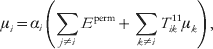$$\mu _{i} \equals \alpha _{i} \left( {\sum\limits_{j \ne i} {E^{{\rm perm}} } \plus \sum\limits_{k \ne i} {T_{ik}^{\setnum{11}} \mu _{k} } } \right)\comma $$

where T ¹¹ is the dipole field operator (e.g. Applequist et al., Reference Applequist, Carl and Fung1972). Since the induced dipole appears on both sides of the equation, it can be solved self-consistently by iteration or by direct matrix inversion. The energy from the mutual induction is

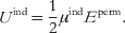$$U^{{\rm ind}} \equals {1 \over 2}\mu ^{{\rm ind}} E^{{\rm perm}} .$$

Although induction always lowers the system energy, the factor ½ reflects the positive work required to distort the molecular charge distribution.

While molecular polarization response is a physical observable, measurable from experiment or computed from ab initio QM, polarization at the atomic level is modeled empirically by inducing a dipole moment at each atom or charge flow between atoms. To model the molecular dipole polarizability, distributed atomic models – both additive and non-additive (interactive) – have been proposed. In an additive model, the molecular polarizability is the sum of individual bond, atom, or group contributions (Dykstra, Reference Dykstra2001). Anisotropic atomic polarizabilities in tensor forms are used to produce anisotropic molecular response (Birge, Reference Birge1980; Stout & Dykstra, Reference Stout and Dykstra1995; Stout & Dykstra, Reference Stout and Dykstra1998). Applequist et al. (Reference Applequist, Carl and Fung1972) devised a non-additive model in which atomic response is relayed via neighboring atoms and, as a result, anisotropic molecular response can be captured (Stout & Dykstra, Reference Stout and Dykstra1995; Stout & Dykstra, Reference Stout and Dykstra1998). Applequist further incorporated monopole polarizability (atomic charge transfer) into the dipole polarizability model to handle out-of-plane charge flow in the aromatic rings (Applequist, Reference Applequist1993). Thole proposed a damping scheme to handle numerical problems in the interactive model associated with the polarizability catastrophe at the short range (polarization energy approaches negative infinity) (Thole, Reference Thole1981; van Duijnen & Swart, Reference Van Duijnen and Swart1998). Physically, the catastrophe is a consequence of point polarizability approximation and the damping is effectively to replace the point charge with a distribution. Thole's approach has been adopted by several researchers in empirical force fields for classical simulations or QM/MM approaches (Åstrand et al., Reference Åstrand, Linse and Karlström1995; Bernardo et al., Reference Bernardo, Ding, Krogh-Jespersen and Levy1994; Brdarski et al., Reference Brdarski, Astrand and Karlstrom2000; Burnham & Xantheas, Reference Burnham and Xantheas2002; Engkvist et al., Reference Engkvist, Åstrand and Karlström1996; Grossfield et al., Reference Grossfield, Ren and Ponder2003; Holt & Karlström, Reference Holt and Karlström2009; Jiao et al., Reference Jiao, King, Grossfield, Darden and Ren2006, Reference Jiao, Golubkov, Darden and Ren2008; Ren & Ponder, Reference Ren and Ponder2002, Reference Ren and Ponder2003; Van Duijnen & de Vries, Reference Van Duijnen and De Vries1996; Xantheas et al., Reference Xantheas, Burnham and Harrison2002). The advantage of additive models is the computational simplicity, whereas the interactive models require the solution of self-consistent mutual induction equations. However, in the interactive polarizability model, the molecular response has explicit dependence of molecular geometry, which is often lacking in the additive models. In addition to the empirical models mentioned above, Stone proposed a more sophisticated distributed polarizability model based on perturbation theory which systematically treats polarization response in monopole to higher-order moments (Stone, Reference Stone1996).

Different methods exist to incorporate the polarization effect in molecular mechanic framework, by means of induced dipole, fluctuating charge or Drude oscillator. The latter two are easier to implement within the existing fixed-charge force field methodology, while the induced dipole approach makes it a natural choice for models based on atomic multipoles. Detailed discussion and comparison of the different treatments of polarization can be found in the recent reviews (Halgren, Reference Halgren1992; Ponder & Case, Reference Ponder and Case2003; Rick, Reference Rick2001). Stone (Stone, Reference Stone1981, Reference Stone2005; Stone & Alderton, Reference Stone and Alderton2002) proposed a more sophisticated treatment.

Efforts to develop classical force fields that explicitly treat the electronic polarization effect are increasing. Ren and Ponder are developing a classical force field that combines the induced dipole with permanent atomic multipoles to represent the electrostatic interactions (Jiao et al., Reference Jiao, Golubkov, Darden and Ren2008; Kong, Reference Kong1997; Ren & Ponder, Reference Ren and Ponder2002, Reference Ren and Ponder2003). Friesner and co-workers also reported models that merge fluctuating charges and atomic induce dipole models together (Kaminski et al., Reference Kaminski, Stern, Berne, Friesner, Cao, Murphy, Zhou and Halgren2002; Stern et al., Reference Stern, Rittner, Berne and Friesner2001). Patel et al. (Patel & Brooks, Reference Patel and Brooks2004; Patel et al., Reference Patel, Mackerell and Brooks2004) take a fluctuating charge approach that is based on the charge equilibration scheme (Rappe & Goddard, Reference Rappe and Goddard1991). MacKerell and Roux base their polarizable potential on the Drude oscillator approach (Lamoureux & Roux, Reference Lamoureux and Roux2006; Lopes et al., Reference Lopes, Lamoureux, Roux and Mackerell2007). In principle, the inclusion of polarization should provide a more realistic representation of electrostatic interactions and better transferability of force field parameters. Ren and co-workers have shown that electronic polarizability needs to be considered in order to achieve reliable and accurate results in small molecules binding to proteins (Jiao et al., Reference Jiao, Golubkov, Darden and Ren2008, Reference Jiao, Zhang, Duke, Li, Schnieders and Ren2009). Polarization allows more rigorous parameterization and validation of the force field against a wide range of molecular systems in different environment, from small molecules to macromolecules, from gas-phase to condensed-phase properties. Of equal importance is the development of efficient particle-mesh Ewald has enabled accurate treatment of long-range electrostatic interactions of partial charges or point multipoles in the simulations of large biomolecules (Darden et al., Reference Darden, York and Pedersen1993; Sagui et al., Reference Sagui, Pedersen and Darden2004). However, developing and parameterizing a consistent force field for biomolecular simulations are still daunting tasks because of the extra complication in a more elaborated physical model. It is also important to keep in mind the limitation of other representations in the potential energy function such as van der Waals interactions and short-range valence term.

4.3 Modeling biomolecular titration states

One of the most important aspects of biomolecular charge states is their sensitivity to pH and other environmental influences. The presence of ionizable groups (side chains of acidic and basic amino acids) in a protein affects the protein's electrostatic properties and its solvation in aqueous media. The two types of ionizable groups in proteins are titratable and redox groups. Titratable groups participate in acid–base (protonation/de-protonation) reactions to exchange (bind or release) a proton. Redox groups participate in redox reactions to exchange (bind or release) an electron. Therefore, these ionizable groups can acquire charge states that determine the stability, solubility, and enzymatic properties of the proteins important in several biological processes (e.g. enzymatic catalysis, respiration, etc.). In fact, several pH-dependent phenomena associated with proteins have been attributed to the presence of titratable groups. To understand the mechanisms of biological phenomena that depend on the ionization states of proteins, it is important to predict accurately these ionization states and understand the factors that affect the ionization behavior of proteins.

The ionization behavior and the corresponding charge state of an ionizable group can be different when it is part of a protein compared to when it exists independently as part of its model compound (side chain in a blocked peptide) in aqueous solutions. Several factors alter the charge state of ionizable groups in a protein: electrostatic interactions between charges of ionizable groups in the same protein, electrostatic interactions between charges on the ionizable group and the partial charges on non-ionizable groups and backbone atoms, location of the group in the protein, changes in the protein's conformational state, pH of the solution, and polarizability/polarity of the protein's microenvironment.

The ionization behavior of an ionizable group (titratable or redox) can be characterized by the proton/electron binding affinities of the titratable/redox group. The binding affinity of a group can change depending on whether the group is part of a protein or is left free in solution. These affinities can be quantified using ionization equilibrium constants. For instance, Equation (5) is for an acid–base equilibrium (protonation/de-protonation) reaction, where AH denotes the acid, A⁻ represents the conjugate base and H⁺ is the proton:

(5)$$AH\buildrel {K_{\alpha } } \over\longleftrightarrow A^{ \minus } \plus H^{ \plus } .$$

K_a is the equilibrium constant, defined as K_a = [A ⁻][H ⁺]/HA, where the terms in the numerator and denominator are species activities, and K_a determines the strength for the dissociation of the acid into its conjugate base and a proton. Taking negative logarithm on both sides of Equation (5) yields

(6)$$ \minus \log _{\setnum{10}} K_{a} \equals \minus \log _{\setnum{10}} \left( {{{\lsqb A^{ \minus } \rsqb } \over {\lsqb HA\rsqb }}} \right) \minus \log _{\setnum{10}} \lsqb H^{ \plus } \rsqb .$$

The free energy (ΔG) required to de-protonate one mole of an acid is given by the relation

(7)$$\rmDelta G \equals \minus 2.303k_{\rm B} T\log _{\setnum{10}} \left( {{{\lsqb A^{ \minus } \rsqb } \over {\lsqb HA\rsqb }}} \right)\comma $$

where k _B is the Boltzmann's constant and T is the temperature of the solution. Rearranging these equations gives

(8)$$\rmDelta G \equals 2.303K_{\rm B} T\lpar \minus \log _{\setnum{10}} k_{a} \plus \log _{\setnum{10}} \lsqb H^{ \plus } \rsqb \rpar .$$

Substituting −log₁₀k _a and −log₁₀ [H⁺] with pK _a and pH, respectively, we obtain the relation between free energy and pK _a

(9)$$\rmDelta G \equals 2.303{\rm \ }k_{\rm B} T\lpar {\rm p}K_{\rm a} \minus {\rm pH}\rpar .$$

The ionization state of a protein is characterized by the pK _a values of all the ionizable groups in the protein. We can write the relation between pK _a (pK _a,i) of a titratable group (i) in a protein (p) and the change in free energy (ΔG_i^p) required to protonate the titratable group, as shown below:

(10)$$\rmDelta G_{i}^{p} \equals 2.303{\rm \ }k_{\rm B} T\lpar {\rm pH} \minus {\rm p}K_{{\rm a}\comma i} \rpar .$$

Similarly, the pK _a (pK _a,mi) of the same titratable group (i) in a reference or model state (m) is related to the change in free energy (ΔG_i^m) required to protonate the titratable group, as shown below:

(11)$$\rmDelta G_{i}^{m} \equals 2.303{\rm \ }k_{\rm B} T\lpar {\rm pH} \minus {\rm p}K_{{\rm a}\comma mi} \rpar .$$

Subtracting these two relationships and rearranging gives

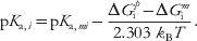(12)$${\rm p}K_{{\rm a}\comma i} \equals {\rm p}K_{{\rm a}\comma mi} \minus {{\rmDelta G_{\rm i}^{ p } \minus \rmDelta G_{\rm i}^{m} } \over {2.303{\rm \ }k_{\rm B} T}}.$$

Equation (12) provides the thermodynamic basis for understanding the differences between the ionization behavior of a titratable group in a protein and that of the same group in its model compound.

A common assumption in pK _a calculations is that the contributions to the free energy of charging a site in the protein or model compound from zero to unit charge (positive or negative) are purely electrostatic in nature (Bashford & Karplus, Reference Bashford and Karplus1990). These electrostatic contributions include the solvation energy of the charge at the ionizable site (Born), the electrostatic interaction between the charge and the partial charges of backbone atoms and other non-ionizable groups (ic–p interactions), and the electrostatic interaction between the charge and charges on other ionizable groups (ic–jc interactions).

Thus, the pK _a of a titratable state becomes

(13)$${\rm p}K_{{\rm a}\comma i} \equals {\rm p}K_{{\rm a}\comma mi} \minus {{\rmDelta G_{i{\rm ,\ Born}}^{p } \plus \rmDelta G_{i,{\rm \ }ic \minus p}^{p } \plus \rmDelta G_{i,{\rm \ }ic \minus jc}^{p } \minus \rmDelta G_{i{\rm , \ Born}}^{m} \minus \rmDelta G_{i,{\rm \ }ic \minus p }^{m} } \over {2.303{\rm \ }k_{\rm B} T}}.$$

To calculate the pK _a,i value of the titratable group i, we need to know the values for pK _a,mi and for each free energy term in equation above. The pK _a,mi value can be obtained experimentally; however, the free energy terms have to be computed using a suitable electrostatic solvation model, as discussed in the subsequent sections. Note that the term ΔG_{i. ic−jc}^p is pH-dependent, which also implies the need to sample against the large space of biomolecular titration states to accurately model the pK _a value (Antosiewicz, Reference Antosiewicz2008).

Significant efforts have been made to accurately measure (Baran et al., Reference Baran, Chimenti, Schlessman, Fitch, Herbst and Garcia-Moreno2008; Castañeda et al., Reference Castañeda, Fitch, Majumdar, Khangulov, Schlessman and García-Moreno2009; Denisov et al., Reference Denisov, Schlessman, García-Moreno and Halle2004; Fitzkee & García-Moreno E, Reference Fitzkee and García-Moreno2008; Harms et al., Reference Harder and Roux2008, Reference Harms, Castañeda, Schlessman, Sue, Isom, Cannon and García-Moreno2009; Isom et al., Reference Isom, Cannon, Castañeda, Robinson and García-Moreno2008, Reference Isom, Castañeda, Cannon, Velu, García-Moreno and García2010, Reference Isom, Castañeda, Cannon and García-Moreno2011; Karp et al., Reference Karp, Gittis, Stahley, Fitch, Stites and Garcia-Moreno2007, Reference Karp, Stahley and García-Moreno2010) and predict (Alexov et al., Reference Alexov, Mehler, Baker, Baptista, Huang, Milletti, Erik Nielsen, Farrell, Carstensen, Olsson, Shen, Warwicker, Williams and Word2011; Antosiewicz et al., Reference Antosiewicz, Briggs, Elcock, Gilson and Mccammon1996a, Reference Breneman and Wibergb, Reference Antosiewicz2008; Bashford & Karplus, Reference Bashford and Karplus1990; Bryce et al., Reference Bryce, Vincent, Malcolm, Hillier and Burton1998; Carstensen et al., Reference Carstensen, Farrell, Huang, Baker and Nielsen2011; Flanagan et al., Reference Flanagan, Ackers, Matthew, Hanania and Gurd1981; Georgescu et al., Reference Georgescu, Alexov and Gunner2002; Karp et al., Reference Karp, Gittis, Stahley, Fitch, Stites and Garcia-Moreno2007; Khandogin & Brooks, Reference Khandogin and Brooks2006; Laurents et al., Reference Laurents, Huyghues-Despointes, Bruix, Thurlkill, Schell, Newsom, Grimsley, Shaw, Treviño, Rico, Briggs, Antosiewicz, Scholtz and Pace2003; Li et al., Reference Li, Hains, Everts, Robertson and Jensen2002, Reference Li, Robertson and Jensen2004, Reference Li, Robertson and Jensen2005; Mehler & Guarnieri, Reference Mehler and Guarnieri1999; Mitra et al., Reference Mitra, Zhang and Alexov2011; Nielsen, Reference Nielsen, Michael and Ludwig2007, Reference Nielsen2009, Reference Nielsen, Gunner and Bertrand García-Moreno2011; Nielsen & McCammon, Reference Nielsen and Mccammon2003; Nielsen & Vriend, Reference Nielsen and Vriend2001; Shan & Mehler, Reference Shan and Mehler2011; Tang et al., Reference Tang, Alexov, Pyle and Honig2007; Tynan-Connolly & Nielsen, Reference Tynan-Connolly and Nielsen2006; Wallace & Shen, Reference Wallace and Shen2011; Witham et al., Reference Witham, Talley, Wang, Zhang, Sarkar, Gao, Yang and Alexov2011) protein titration states to understand the determinants of pK _a values for the amino acids in the interior and exterior of proteins. A recent special issue of Proteins (Alexov et al., Reference Alexov, Mehler, Baker, Baptista, Huang, Milletti, Erik Nielsen, Farrell, Carstensen, Olsson, Shen, Warwicker, Williams and Word2011) provides an excellent review of the state-of-the-art in the area of biomolecular titration state modeling.

5.1 Explicit water models

Water has long been recognized as an important part of biomolecular systems (Kauzmann, Reference Kauzmann1959). Early theoretical studies of proteins ignored the solvent because of the prohibitive computational cost (McCammon et al., Reference Mccammon, Gelin and Karplus1977). However, with the advancement of computer technology and quest for realistic simulations, it is now common to represent the solvent explicitly with atomic models.

Numerous water models have been developed over the years beginning with Bernal and Fowler's attempt in 1933 (Bernal, Reference Bernal1933). A detailed review of nearly 50 water models was given by Guillot in 2002 (Guillot, Reference Guillot2002). It would likely require another full-length review to discuss the new models developed since. The water models introduced to date differ from each other in electrostatic representation (number of charge sites, polarizability), internal geometry (angle and flexibility), and the ways by which the parameters were derived.

TIP3P (Jorgensen et al., Reference Jorgensen, Chandrasekhar, Madura, Impey and Klein1983) and Simple Point Charge (SPC) (Berendsen et al., Reference Berendsen, Postma, Van Gunsteren, Hermans and Pullmann1981) are two, three-site, fixed charge models commonly used in biomolecular simulations. The two models have the same equilibrium OH bond lengths and very similar atomic charges but different van der Waals parameters and equilibrium HOH angle values. While the TIP3P adopts a value of 104.52° for the HOH angle, SPC uses 109.47°; the experimentally measured geometry of liquid water at room temperature is 106° (Ichikawa et al., Reference Ichikawa, Kameda, Yamaguchi, Wakita and Misawa1991). Both water models were derived originally as rigid water models. A variant of SPC, SPC/E (Berendsen et al., Reference Berendsen, Grigera and Straatsma1987), was developed to take into account the cost of bulk polarization ignored by SPC and other fixed-charge models. Effectively, the correction makes the bulk potential energy of SPC/E model lower than the others. This procedure has not been consistently applied to other liquids or biomolecular systems.

The effort to improve TIP3P has led to four-site (Jorgensen et al., Reference Jorgensen, Chandrasekhar, Madura, Impey and Klein1983), five-site (Mahoney & Jorgensen, Reference Mahoney and Jorgensen2000), and even six-site (Nada, Reference Nada2003) water models, with additional charge sites for better electrostatic descriptions. An extensive reparameterization of TIP4P was made by fitting to properties over a wide range of temperatures and using the Ewald treatment of electrostatics, as opposed to the cut-off scheme used in earlier model development (Horn et al., Reference Horn, Swope, Pitera, Madura, Dick, Hura and Head-Gordon2004). TIP5P is one of the best-performing fixed charge water models that reproduce a range of condensed-phase structural, energetic, and dynamic properties including the temperature of maximum density. The use of TIP5P in biomolecular simulations has been limited because of the cost arising from the additional charge sites and concerns about compatible parameterization of amino and nucleic acid residues with this water model.

Recent advancements in water models continue to focus on the electrostatic representation, especially the electronic polarization effect. Water is a high-dielectric solvent and is also very polarizable itself. Examples of water models that explicitly account for polarization include a water model developed by Brodholt, Sampoli and Vallauri (BSV) (Jedlovszky, Reference Jedlovszky2001; Jedlovszky & Vallauri, Reference Jedlovszky and Vallauri1999), Polarizable five-site model, based on triple zeta basis set (POL5/TZ)(QZ) (Stern et al., Reference Stern, Rittner, Berne and Friesner2001), Polarizable Point-Charge (PPC) (Svishchev et al., Reference Svishchev, Kusalik, Wang and Boyd1996), transferable intermolecular potential, 4-position model/Fluctuation Charge (TIP4P/FQ) (Rick, Reference Rick2001), POL5 (Stern et al., Reference Stern, Rittner, Berne and Friesner2001), Thole-Type Model, version 2 (TTM2) (Burnham & Xantheas, Reference Burnham and Xantheas2002), Atomic Multipole Optimized Energetics for Biomolecular Applications (AMOEBA) (Ren & Ponder, Reference Ren and Ponder2003), and SWM4-DP (Lamoureux et al., Reference Lamoureux, Mackerell and Roux2003). Parameterization of these models relies on both quantum mechanical ab initio calculations and experimental bulk thermodynamic properties, although to different extents. Overall, these studies have demonstrated that a polarizable water model is able to provide a better representation of electrostatic response, and good transferability among different chemical environments.

5.2 Explicit ion models

When explicit water models are used, ions are also typically modeled in atomic detail. Theoretical treatment of specific ion interactions is complicated as the strong electrostatic field around the ions poses challenges to the standard physical water models. Nonetheless, computational studies have offered valuable insights into the atomic details of ion solvation and the interaction of ions with biomolecular solutes.

Specific ion binding to proteins or DNA is a dynamic competition between the biomolecular and aqueous environments. Therefore, it is essential to accurately describe the hydration thermodynamics of single ions. However, this task is not straightforward as only the total solvation free energies of a neutral salt can be measured directly from experiment. As a result, published single ion solvation values differ widely when different parameterizations are employed (Patra & Karttunen, Reference Patra and Karttunen2004). Furthermore, ion behavior can be very sensitive to the force field, and subtle differences in ion and solvent parameterization may lead to significant ion pairing and clustering problems during simulation (Alejandre & Hansen, Reference Alejandre and Hansen2007; Auffinger et al., Reference Auffinger, Cheatham and Vaiana2007; Chen & Pappu, Reference Chen and Pappu2007a, Reference Chen and Pappub; Joung & Cheatham, Reference Joung and Cheatham2008).

Recent studies using ab initio QM/MM models, quasi-chemical theory, and polarizable force fields have demonstrated improved accuracy in explicit ion models. The ab initio QM/MM approach has been reviewed extensively (Friesner, Reference Friesner2005; Friesner & Guallar, Reference Friesner and Guallar2005; Hu & Yang, Reference Hu and Yang2008; Kamerlin et al., Reference Kamerlin, Haranczyk and Warshel2009; Lin & Truhlar, Reference Lin and Truhlar2007; Riccardi et al., Reference Riccardi, Schaefer, Yang Yu, Ghosh, Prat-Resina, König, Li, Xu, Guo, Elstner and Cui2006; Senn & Thiel, Reference Senn and Thiel2009). For example, Rode and co-workers have characterized the dynamics and solvation properties of solvated ions by treating the primary region of interest, the first hydration shell of the ions, quantum mechanically and other region using MM (Azam et al., Reference Azam, Hofer, Randolf and Rode2009; Rode et al., Reference Rode, Hofer, Randolf, Schwenk, Xenides and Vchirawongkwin2006). Unfortunately, most QM/MM calculations are restricted to small systems or short trajectories since quantum mechanical calculations are extremely expensive.

Aqvist has pioneered the work of applying free energy perturbation (FEP) approaches to derive ion–water potential parameters that can reproduce the experimental solvation free energies of alkali and alkaline earth metal ions in water (Aaqvist, Reference Aaqvist1990). While there are still efforts to push the limits of the additive non-polarizable force fields for ionic interactions (Joung & Cheatham, Reference Joung and Cheatham2008), it is generally accepted that polarizability and perhaps even quantum mechanical treatments are essential for accurate descriptions of ion behavior (Halgren & Damm, Reference Halgren and Damm2001) in aqueous solutions (Chang & Dang, Reference Chang and Dang2006; Grossfield et al., Reference Grossfield, Ren and Ponder2003; Lamoureux & Roux, Reference Lamoureux and Roux2006; Stuart & Berne, Reference Stuart and Berne1996) and for more complex environments such as ion–protein interactions (Li et al., Reference Li, Zhang, Wang and Wang2008) and ion channels (Allen et al., Reference Allen, Kuyucak and Chung2000; Bucher et al., Reference Bucher, Raugei, Guidoni, Dal Peraro, Rothlisberger, Carloni and Klein2006; Illingworth & Domene, Reference Illingworth and Domene2009; Noskov et al., Reference Noskov, Im and Roux2004; Roux et al., Reference Roux, Allen, Bernèche and Im2004; Warshel et al., Reference Warshel, Kato and Pisliakov2007).

Several groups have performed molecular dynamics simulations using polarizable force fields to study ion behavior or to determine ion solvation energies. For example, Dang and co-workers used many-body polarizable potential models in molecular dynamics simulations to study the solvation behavior of Li⁺, Na⁺, Cl⁻, and F⁻ in water clusters (Dang, Reference Dang1992; Dang et al., Reference Dang, Rice, Caldwell and Kollman1991) and the significant role that polarization plays in ion binding to the liquid/vapor interface (Chang & Dang, Reference Chang and Dang2006; Dang & Chang, Reference Dang and Chang2001). A protein Langevin dipole model, developed by Aqvist and Warshel (Aqvist & Warshel, Reference Aqvist and Warshel1989) has been used to calculate the solvation energy of a Na⁺ ion inside the Gramicidin A channel and in water, and similar methods have been applied to model the polarization effect in the KcsA channel (Burykin et al., Reference Burykin, Kato and Warshel2003; Luzhkov & Åqvist, Reference Luzhkov and Åqvist2000). Additionally, a polarizable molecular mechanic model based on induced dipole approach was successfully applied to study the absolute solvation free energies for K⁺, Na⁺, and Cl⁻ (Grossfield et al., Reference Grossfield, Ren and Ponder2003), as well as Mg²⁺ and Ca²⁺ (Jiao et al., Reference Jiao, King, Grossfield, Darden and Ren2006). Using a Drude oscillator model for polarizability, Roux and co-workers have developed a polarizable potential function for the hydration of alkali halide salts (Lamoureux & Roux, Reference Lamoureux and Roux2006; Whitfield et al., Reference Whitfield, Varma, Harder, Lamoureux, Rempe and Roux2007), which gives results consistent with ab initio calculations. In addition, the fluctuating charge method of polarization has been applied to ionic systems (Bryce et al., Reference Bryce, Vincent, Malcolm, Hillier and Burton1998; Ribeiro, Reference Ribeiro1999) and has been used to extend classical force fields to include polarization effects (Patel & Brooks, Reference Patel and Brooks2004; Patel et al., Reference Patel, Mackerell and Brooks2004; Warren & Patel, Reference Warren and Patel2007). Despite all these efforts, modeling explicit ions remains a considerable challenge, owing to the complex, dynamic, and subtle nature of ions, and it is expected that the future direction will be focused on using ab initio treatment and polarizable force fields.

6.1 Solvent distributions from integral equations

As discussed above, modeling explicit solvent effects via computer simulation techniques can be costly since the resulting systems involve a large number of particles with long-range interactions and demand substantial computational resources. An alternative route to solvation is provided by integral equation theories (IETs), which simplify the all-atom description of explicit solvation into a probabilistic treatment of distributions between solute and solvent. As a result of this simplification, these methods generally require less computational expense than explicit solvent methods, but offer more detail than the continuum models discussed below (Attard, Reference Attard2002; Hansen & McDonald, Reference Hansen and Mcdonald2000; Hirata, Reference Hirata2003). Because of this compromise, IETs can be efficient and powerful tools to predict the three-dimensional (3D) spatial organization of the solvent density around large molecular solutes of irregular shape as well as related thermodynamic solvation quantities (Beglov & Roux, Reference Beglov and Roux1997; Chandler et al., Reference Chandler, Mccoy and Singer1986; Du et al., Reference Du, Beglov and Roux2000; Harano et al., Reference Harano, Imai, Kovalenko, Kinoshita and Hirata2001; Imai et al., Reference Imai, Harano, Kovalenko and Hirata2001; Kovalenko & Hirata, Reference Kovalenko and Hirata1998, Reference Kovalenko and Hirata1999, Reference Kovalenko and Hirata2000a, Reference Kovalenko and Hiratab, Reference Kovalenko and Hiratac). A particularly popular set of integral equations are the interaction site models (Chandler, Reference Chandler1978; Hirata, Reference Hirata2003; Rossky et al., Reference Rossky, Pettitt and Stell1983) that specifically model the probability distribution of specific atomic sites on the solvent around atomic sites on the solute. The 1D-RISM (reference interaction site model) theory provides site–site radial distribution functions coming from an angular average over the orientation of both solute and solvent molecules (see Fig. 3). This approach has been successfully applied to small molecules in general (Chuev & Fedorov, Reference Chuev and Fedorov2004; Du et al., Reference Du, Beglov and Roux2000, Reference Du, Liu and Huang2008; Freedman & Truong, Reference Freedman and Truong2004; Frolov et al., 2000, Reference Frolov, Ratkova, Palmer and Fedorov2011; Imai et al., Reference Imai, Hiraoka, Kovalenko and Hirata2007a, Reference Imai, Hiraoka, Seto, Kovalenko and Hiratab; Kiyota et al., Reference Kiyota, Hiraoka, Yoshida, Maruyama, Imai and Hirata2009, Reference Kiyota, Yoshida and Hirata2011; Kovalenko & Hirata, Reference Kovalenko and Hirata1998, Reference Kovalenko and Hirata1999, Reference Kovalenko and Hirata2000a, Reference Kovalenko and Hiratab, Reference Kovalenko and Hiratac; Maruyama et al., Reference Maruyama, Yoshida and Hirata2010; Miyata & Hirata, Reference Miyata and Hirata2008; Nishiyama et al., Reference Nishiyama, Yamaguchi and Hirata2009; Stumpe et al., Reference Stumpe, Blinov, Wishart, Kovalenko and Pande2011; Woelki et al., Reference Woelki, Kohler, Krienke and Schmeer2008; Yoshida et al., Reference Yoshida, Phongphanphanee, Maruyama, Imai and Hirata2006). Unlike the 1D model, 3D-RISM keeps the orientational dependence of solute molecules, which is necessary to properly describe solvation properties of large molecular solutes. This more accurate 3D integral equation demands a higher computational cost when compared with the 1D theories (Perkyns & Pettitt, Reference Perkyns and Pettitt1992). It provides not only an accurate site–site radial pair correlation functions but also the correct dielectric properties of polar liquids, which is a key element to properly describe the solvent effects on solutes. Integral equations specify formulae for the total and direct solvent correlation functions. Once solved, these quantities can be used to calculate the solvation chemical potential (Imai et al., Reference Imai, Kovalenko and Hirata2004; Kovalenko & Hirata, Reference Kovalenko and Hirata1999), the potential of mean force for solutes degrees of freedom (Kovalenko & Hirata, Reference Kovalenko and Hirata1999, Reference Kovalenko and Hirata2000b, Reference Kovalenko and Hiratac), solvation coordination numbers (Kovalenko & Hirata, Reference Kovalenko and Hirata1998) and hydration shells (Imai et al., Reference Imai, Hiraoka, Kovalenko and Hirata2007a), hydrophobic effects (Howard et al., Reference Howard, Perkyns, Choudhury and Pettitt2008; Kovalenko & Hirata, Reference Kovalenko and Hirata2000a), as well as many other quantities.

Fig. 3.

This figure represents the solute–solvent site–site pair correlation functions g _uv(r) as a function of the separation distance r predicted by 1D-RISM for N-methyl acetamide immersed in water at infinite dilution. For instance, g _NO(r) is the pair correlation function for a nitrogen atom in N-methyl acetamide molecule and an oxygen atom in water molecule.

Despite the successes achieved by IETs in predicting solvation properties, there remain deficiencies that need to be corrected. A serious problem associated with these approaches is that, when they fail to yield physically reasonable predictions, there are no straightforward, systematic methods to improve IET predictive accuracy. A useful avenue to remedy this situation has been to construct thermodynamically consistent integral equation theories for interaction site fluids in which the optimal closure approximation is determined by first principles (Marucho et al., Reference Marucho, Kelley and Pettitt2008; Marucho & Pettitt, Reference Marucho and Pettitt2007). The re-analysis of the interaction-site formalism has also led to the development of more sophisticated (diagrammatically proper) integral equations eliminating diagrams that are not present in the exact theory (Marucho et al., Reference Marucho, Kelley and Pettitt2008; Marucho & Pettitt, Reference Marucho and Pettitt2007). Another challenge for IETs lies in the inclusion of solute flexibility; however, some progress has been made in this area. IETs can be properly combined with other methodologies such as Monte Carlo simulations which project solvent degrees of freedom onto the solute at the level of site–site pair correlation functions (Freedman & Truong, Reference Freedman and Truong2004; Kinoshita et al., Reference Kinoshita, Okamoto and Hirata1999; Kovalenko & Hirata, Reference Kovalenko and Hirata2000b, Reference Kovalenko and Hiratac). Alternatively, dynamical solute processes in solution can be treated by incorporating the IETs into a generalized Langevin equation, which describes the time evolution of solvent densities (Chong & Hirata, Reference Chong and Hirata1998).

6.2 Ion distributions from integral equations and density functional theories

Like solvent, ion distributions can also be modeled by IETs; for example, by the DRISM introduced in section above, which has been shown to account for changes in the water structure caused by the addition of salts near a protein and associated changes in the solvation free energy from the evaluation of site–site total and direct correlation functions (Imai et al., Reference Imai, Miyashita, Sugita, Kovalenko, Hirata and Kidera2000; Perkyns & Pettitt, Reference Perkyns and Pettitt1994, Reference Perkyns and Pettitt1995, Reference Perkyns and Pettitt1996). While more computationally efficient, the 1D RISM theory suffers from its inability to model the solvent inaccessibility of buried solute atoms accurately. There have been several efforts to correct this problem (Imai et al., Reference Imai, Miyashita, Sugita, Kovalenko, Hirata and Kidera2000); however, the 3D RISM theory described above is somewhat more computationally expensive but free from this problem and provides more accurate predictions of ionic behavior (Imai et al., Reference Imai, Kovalenko and Hirata2004; Yonetani et al., Reference Yonetani, Maruyama, Hirata and Kono2008).

Classical density functional theory (DFT) (Chandler et al., Reference Chandler, Mccoy and Singer1986) provides another powerful tool for describing ionic behaviors through ion distributions. This approach is based on the simple thermodynamic principle that the system reaches the equilibrium as its grand canonical potential reaches minimum. In particular, for a fluid subject to an arbitrary potential V _ext(r, Ω), the grand canonical free energy can be written as a functional of the one-particle density. This free energy functional is minimized at the thermodynamic equilibrium density. Thus, its knowledge of this functional and the equilibrium density characterize the fluid completely. However, this functional is not known for most complex systems and, instead, is approximated in various ways. Different approaches and approximations based on DFT have been proposed to evaluate the excess free energy and the density profile depending on the complexity and features of the system. For example, Gao and co-workers (Wang et al., Reference Wang, Yu and Gao2004) use the weighted-density approximation to describe the structure and thermodynamics properties of small ions around a polyelectrolyte immersed in a continuum media, observing the charge inversion phenomena of DNA at moderate concentrated solution. Ramirez & Borgis (Reference Ramirez and Borgis2005) use the homogeneous reference fluid approximation to develop a general approach that includes the microscopic structure of the solvent, the dipolar saturation effects, and the non-local character of the dielectric constant in the calculation of the average solvent structure solvation properties of molecular solutes of irregular shape. Eisenberg and co-workers (Gillespie et al., Reference Gillespie, Nonner and Eisenberg2002) combine a 1D drift–diffusion (Poisson–Nernst–Planck or, PNP) transport system and DFT to model ion transport in biological ion channels. These examples show the theoretical versatility of DFT for describing ionic solvation in complex systems. However, the same energy functional may not be accurate for all applications and systematic improvements of the functional are not generally possible, instead requiring ad hoc corrections.

7.1 The Poisson equation for polar solvation

The Poisson equation is a fundamental equation of continuum electrostatics (Bottcher, Reference Bottcher1952; Jackson, Reference Jackson1975). It is a linear second-order partial differential equation

$$ \minus \nabla \cdot \lpar \varepsilon \lpar \hskip1pt \vec{r}\hskip2pt\rpar \nabla \phi \lpar \hskip1pt\vec{r}\hskip2pt\rpar \rpar \equals \rho \lpar \hskip1pt \vec{r}\hskip2pt\rpar \quad \quad {\rm for}\;\vec{r} \in \rmOmega \comma $$

which expresses the ESP φ terms of a dielectric coefficient ε and a charge distribution ρ for all points r in some domain Ω. This differential equation must be combined with additional constraints on the potential in order to provide well-posed solutions. These constraints usually take the form of boundary conditions specifying the value of the potential or its derivatives on the boundary ∂Ω of the domain. The most common boundary conditions for biomolecular electrostatics problems are the simple Dirichlet condition which constrains the potential to an asymptotic approximation on the boundary of the domain.

The biomolecular structure and chemistry are introduced into the Poisson equation through the dielectric and charge coefficients. The charge distribution is often represented by a sum of atomic monopoles or higher-order multipoles as described in the ‘Modeling biomolecular charge distributions’ section. The dielectric coefficient is generally a sharply varying function that assumes bulk solvent values outside of the biomolecular surface and other values inside the biomolecule. The value of the dielectric coefficient determines the polarization response of the material when subject to an electric field; more easily polarizable materials have higher dielectric values. While the bulk values of the dielectric are straightforward to determine, based on the properties of the homogeneous solvent, the dielectric values inside the biomolecule are much more difficult to interpret and have been subject to much debate and analysis (Roux, Reference Roux1999; Schutz & Warshel, Reference Schutz and Warshel2001; Sham et al., Reference Sham, Muegge and Warshel1998; Simonson, Reference Simonson1999, Reference Simonson2001, Reference Simonson2003, Reference Simonson2008; Teixeira et al., Reference Teixeira, Cunha, Machuqueiro, Oliveira, Victor, Soares and Baptista2005; Tjong & Zhou, Reference Tjong and Zhou2008). In particular, the choice of internal dielectric coefficient values is usually very dependent on the specific application. If the only polarization response of the biomolecular interior results from electronic reorganization, then the most appropriate value of the biomolecular dielectric coefficient should be between 2 and 4 (Landau et al., Reference Landau, Lifshitz and Pitaevskii1982). Such low dielectric models are appropriate for simulations and calculations such as MM/PBSA (MM/PB surface area) where the molecular flexibility of the molecule is modeled explicitly through conformational sampling. Higher values of the internal biomolecular dielectric are intended to mimic additional relaxation properties, including orientational changes in molecular dipoles, side-chain rearrangement, and even penetration of water into the biomolecular interior. Values from 4 to 20 have been regularly used in a variety of biomolecular applications with lower values generally being successful for protein–ligand interactions (Kollman et al., Reference Kollman, Massova, Reyes, Kuhn, Huo, Chong, Lee, Lee, Duan, Wang, Donini, Cieplak, Srinivasan, Case and Cheatham2000; Massova & Kollman, Reference Massova and Kollman2000), moderate values of 10–12 necessary for protein–protein binding energies (Elcock et al., Reference Elcock, Sept and Mccammon2001), and values 20 or higher needed for titration state and pK _a predictions (Chimenti et al., Reference Chimenti, Castañeda, Majumdar and García-Moreno2011; Schutz & Warshel, Reference Schutz and Warshel2001).

In addition to the variety of dielectric coefficient values, there are also many choices available for the functional form and shape of the biomolecule-solvent dielectric boundary (see Fig. 4) (Chen et al., Reference Chen, Baker and Wei2010, Reference Chen, Baker and Wei2011b; Grant & Pickup, Reference Grant and Pickup1995; Grant et al., Reference Grant, Pickup and Nicholls2001; Im, Reference Im1998; Tjong & Zhou, Reference Tjong and Zhou2008). The results of most biomolecular solvation and electrostatics calculations are very sensitive to the definition of this boundary, so it is not surprising that the optimal choice of biomolecular parameters and dielectric value are dependent on the particular dielectric boundary of choice (Nina et al., Reference Nina, Im and Roux1999; Swanson et al., Reference Swanson, Wagoner, Baker and Mccammon2007). As with the dielectric value, the choice of a particular boundary geometry is dependent on many factors, including the specific problem under consideration, the original geometry definitions used to optimize the parameters desired for the given calculation. The most popular biomolecular dielectric interface definition is the molecular surface (Connolly, Reference Connolly1983, Reference Connolly1985) which was used to parameterize the PARSE parameter set for biomolecular solvation calculations (Sitkoff et al., Reference Sitkoff, Sharp and Honig1994a, Reference Sitkoff, Sharp and Honigb). Zhou and co-workers have suggested the use of van der Waals surface as an alternative to the molecular surface for several different applications (Dong et al., Reference Dong, Vijayakumar and Zhou2003; Tjong & Zhou, Reference Tjong and Zhou2008). Both the molecular and van der Waals surfaces can introduce significant conformational sensitivity that can be problematic for applications that explicitly sample different conformational states. As a result, a number of smoother surfaces have also been introduced, including Gaussian (Grant et al., Reference Grant, Pickup and Nicholls2001; Grant & Pickup, Reference Grant and Pickup1995) and spline-based representations (Im, Reference Im1998; Schnieders et al., Reference Schnieders, Baker, Ren and Ponder2007). These surfaces require a distinct set of parameters for accurate calculations, as described (Grant et al., Reference Grant, Pickup and Nicholls2001, Reference Grant, Pickup, Sykes, Kitchen and Nicholls2007; Grant & Pickup, Reference Grant and Pickup1995) for Gaussian interfaces and by others (Nina et al., Reference Nina, Im and Roux1999; Swanson et al., Reference Swanson, Wagoner, Baker and Mccammon2007) for spline-based representations. Finally, new generations of molecular surface definitions that are designed to minimize noise from topological artifacts (Bajaj, Reference Bajaj2003; Zhang et al., Reference Zhang, Xu and Bajaj2006) and to provide a clear physical basis for coupling to non-polar representations (Chen et al., 2010, Reference Chen, Baker and Wei2011b; Dzubiella & Hansen, Reference Dzubiella and Hansen2004; Dzubiella et al., Reference Dzubiella, Swanson and Mccammon2006a, Reference Dzubiella, Swanson and Mccammonb) are appearing. In particular, new surfaces based on geometric flow (Chen et al., 2001, Reference Chen, Baker and Wei2010) provide a self-consistent description of the biomolecular interface that is compatible with the continuum polar and non-polar energy functions. While these new surfaces appear very promising, they will require parameterization before they can be used optimally in biophysical calculations.

Fig. 4.

Images of the varying definitions for the biomolecular surface of fasciculin-2 (PDB ID: 1FAS) with ESP shown ranging from −5 kT/e (dark red) to +5 kT/e (dark blue). (A) van der Waals surface. (B) Solvent-excluded, molecular, or Connolly surface. (C) Solvent-accessible surface.

The linear and local nature of the dielectric coefficient introduce two major assumptions into the model (Beglov & Roux, Reference Beglov and Roux1996, Reference Beglov and Roux1997). Linear response implies a proportional increase in system polarization for all strengths of electric field. This approximation clearly breaks down near highly charged interfaces (e.g. nucleic acids or strongly charged proteins) where dielectric saturation and electrostriction processes can become important. Several models have been developed to provide for non-linear response, generally in the form of a Langevin response function (Azuara et al., Reference Azuara, Orland, Bon, Koehl and Delarue2008; Papazyan & Warshel, Reference Papazyan and Warshel1997, Reference Papazyan and Warshel1998). The second major approximation is the local nature of the dielectric constant which implies that local changes in the electric field have only local influences on polarization. However, the molecular nature of water and its associated network of hydrogen bonding and extended structure at interfaces clearly indicate that this approximation is incorrect, particularly at very small (molecular) length scales. Non-local features have also been introduced into the Poisson equation, but incur increased computational expense (Bardhan, Reference Bardhan2011; Basilevsky & Parsons, Reference Basilevsky and Parsons1998; Rottler & Krayenhoff, Reference Rottler and Krayenhoff2009).

7.2 The PB equation for polar solvation

The Poisson equation only includes the influence of solvent on the electrostatic properties of a solute. However, as discussed in earlier sections of this review, mobile ions also play a very important role on biomolecular electrostatics and solvation. The PB model was developed to address the need to include simple effects from low valency ions in dilute solutions (Baker, Reference Baker2004, Reference Baker2005a, Reference Bakerb; Baker et al., Reference Baker, Bashford, Case, Barth, Griebel, Keyes, Nieminen, Roose, Schlick, Leimkuhler, Chipot, Elber, Laaksonen, Mark, Schütte and Skeel2006; Davis & McCammon, Reference Davis and Mccammon1990; Dong et al., Reference Dong, Olsen and Baker2008; Grochowski & Trylska, Reference Grochowski and Trylska2008; Honig & Nicholls, Reference Honig and Nicholls1995; Honig et al., Reference Honig, Hubbell and Flewelling1986; Sharp & Honig, Reference Sharp and Honig1990a, Reference Sharp and Honigb). One of the best reviews of the model and its caveats was written by Fixman (Fixman, Reference Fixman1979). The PB model essentially relates the local ESP to the average mobile charge densities. Several important approximations are associated with the PB model (Baker, Reference Baker2004; Beglov & Roux, Reference Beglov and Roux1996, Reference Beglov and Roux1997; Fixman, Reference Fixman1979; Holm et al., Reference Holm, Kekicheff and Podgornik2001).

The first approximation, similar to the Poisson equation, is that system solution can be described a continuum, including the dielectric response described above as well as an average density of point-like ions. This density model precludes the treatment of site-specific ion–solute interactions as well as other phenomena that involve details of ionic shape. The PB model cannot explain differences between ion species in solution and thereby prevents effective analysis of specific ion species and the associated phenomena described earlier in this review.

The second approximation models the distribution of ions in terms of single-species average distribution functions. In other words, ions interact with each other only through their average densities rather than through the steric, Coulombic, and solvent-mediated correlations that occur in real electrolyte systems. As a consequence, the PB model cannot capture a number of phenomena (Chen & Weeks, Reference Chen and Weeks2006; Savelyev & Papoian, Reference Savelyev and Papoian2007; Tan & Chen, Reference Tan and Chen2005), including charge inversion (Besteman et al., Reference Besteman, Zevenbergen, Heering and Lemay2004, Reference Besteman, Zevenbergen and Lemay2005; Goel et al., Reference Goel, Patra, Ghosh and Mukherjee2008; Kim & Sung, Reference Kim and Sung2005; Luan & Aksimentiev, Reference Luan and Aksimentiev2010; Martin-Molina et al., Reference Martin-Molina, Calero, Faraudo, Quesada-Perez, Travesset and Hidalgo-Alvarez2009; Nguyen et al., Reference Nguyen, Grosberg and Shlovskii2000; Qiao & Aluru, Reference Qiao and Aluru2004; Taheri-Araghi & Ha, Reference Taheri-Araghi and Ha2005; Wen & Tang, Reference Wen and Tang2004) and like-charge attraction (Angelini et al., Reference Angelini, Liang, Wriggers and Wong2003; Kim et al., Reference Kim, Yi and Pincus2008; Mukherjee, Reference Mukherjee2004; Netz & Naji, Reference Netz and Naji2004; Pietronave et al., Reference Pietronave, Arcesi, D'Arrigo and Perico2008; Podgornik & Dobnikar, Reference Podgornik and Dobnikar2001; Qiu et al., Reference Qiu, Parsegian and Rau2010; Todd et al., Reference Todd, Parsegian, Shirahata, Thomas and Rau2008; Zelko et al., Reference Zelko, Iglič, Iglič and Kumar2010) that can be important for highly charged systems. Such systems include solutes such as DNA, charged biomembrane interfaces, and solutions with even moderate concentrations of di- or multi-valent ions. Ionic correlations and fluctuation corrections have been considered in previous studies. Based on the Kirkwood hierarchy (Kirkwood, Reference Kirkwood1934), a fluctuation potential and an excluded-volume factor have been added to the potential of mean force to represent the effect of ion correlations (Burley et al., Reference Burley, Hutson and Outhwaite1974; Carnie & Torrie, Reference Carnie and Torrie2007; Grochowski & Trylska, Reference Grochowski and Trylska2008). The fluctuation potential is associated with the energy for charging ions and implicitly takes into account the inter-ion Coulomb correlations. This modification provides improved predictions for ion distribution and mean ESP profile with multivalent ions, as compared with the conventional PB model (Carnie & Torrie, Reference Carnie and Torrie2007). However, since the fluctuation potential itself is coupled to the ESP, the 3D numerical solution becomes computationally very expensive and is impractical for applications such as nucleic acid structures (Gavryushov, Reference Gavryushov2008). Other approaches such as the density functional and integral equation methods were discussed earlier; however, the computational complexity for these approaches is still problematic for many applications.

Another important approximation involves the assumption of infinitesimal ion size which can produce arbitrarily large ion concentrations near highly charged solutes. Borukhov et al. (Reference Borukhov, Andelman and Orland1997) developed a simple analytical approach to include the finite ion size in the original PB model. The modified formula was developed for asymmetric and symmetric electrolytes and matched with the original PB equation when an ionic concentration is low. The size effect was introduced as additional correction terms in the entropic contribution of the total free energy. Such corrections were employed by considering the lattice gas formalism, where each lattice site is occupied at most by one ion; the standard PB model corresponds to one with unlimited number of ions in each lattice site. A similar approach based on the lattice gas formalism was used in other studies (Borukhov et al., Reference Borukhov, Andelman and Orland2000; Chaudhry et al., Reference Chaudhry, Bond and Olson2011; Coalson et al., Reference Coalson, Walsh, Duncan and Tal1995; Coalson & Duncan, Reference Coalson and Duncan1992) to incorporate the finite size effect. This size-modified PB model showed appreciable improvements in predictions for ion-binding properties of monovalent counterions, especially at high-salt concentration, which involves the saturation effect for ion binding. However, the consideration of the finite ion size still cannot capture the binding of the divalent and multivalent ions, which may be because of the absence of ion–ion correlations (Chu et al., Reference Chu, Bai, Lipfert, Herschlag and Doniach2007).

Despite the caveats and approximations described above, the PB model is simple and captures enough basic solvation behavior to be a popular choice for describing many biomolecular systems. While there are many more interesting ways to drive the PB equation (Holm et al., Reference Holm, Kekicheff and Podgornik2001), the simplest method starts with the Poisson equation, repeated here:

$$ \minus \nabla \cdot \lpar \varepsilon \lpar \hskip1pt\vec{r}\hskip2pt\rpar \nabla \phi \lpar \hskip1pt\vec{r}\hskip2pt\rpar \rpar \equals \rho \lpar \hskip1pt\vec{r}\hskip2pt\rpar .$$

In the Poisson discussion above, we considered only a single contribution to the charge density $\rho \lpar \hskip1pt\vec{r}\hskip2pt\rpar $ due to the solute. For the PB equation, the charge distribution is assumed to consist of two separate contributions: the solute charges $\rho _{s} \lpar \hskip1pt\vec{r}\hskip2pt\rpar $ and the mobile ions in an aqueous medium $\rho _{m} \lpar \hskip1pt\vec{r}\hskip2pt\rpar $. The charge distribution of the solute was discussed previously; for a simple monopole approximation, the charges Q_i located at each solute atom's position r_i can be modeled via a delta function:

$$\rho _{s} \lpar \hskip1pt\vec{r}\hskip2pt\rpar \equals \sum\limits_{i} {Q_{i} \delta \lpar \hskip1pt\vec{r} \minus \vec{r}_{i} \rpar } .$$

For a mean-field approximation, the charge distribution associated with the mobile ions can be described by a Boltzmann distribution. For m ion species with charges q_j, bulk concentration c_j^b and steric potential $V_{j} \lpar \hskip1pt\vec{r}\hskip2pt\rpar $ (a potential to describe non-polar interactions with the solute), the charge for the mobile ions is

$$\rho _{m} \lpar \hskip1pt\vec{r}\hskip2pt\rpar \equals \mathop \sum \limits_{j}^{m} c_{j}^{b} q_{j} {\rm exp}\left[ {{{ \minus q_{j} \phi \lpar \hskip1pt\vec{r}\hskip2pt\rpar } \over {k_{\rm B} T}} \minus {{V_{j} \lpar \hskip1pt\vec{r}\hskip2pt\rpar } \over {k_{\rm B} T}}} \right]\comma $$

where k _B is the Boltzmann's constant and T is the system temperature. Substituting the two charge distributions into the Poisson equation, one obtains the full PB equation:

$$ \minus \nabla \cdot \lpar \varepsilon \lpar \hskip1pt\vec{r}\hskip2pt\rpar \nabla \phi \lpar \hskip1pt\vec{r}\hskip2pt\rpar \rpar \equals \mathop \sum \limits_{i}^{N} Q_{i} \delta \lpar \vec{r} \minus \vec{r}_{i} \rpar \plus \mathop \sum \limits_{j}^{m} c_{j}^{b} q_{j} {\rm exp}\left[ {{{ \minus q_{j} \phi \lpar \hskip1pt\vec{r}\hskip2pt\rpar } \over {k_{\rm B} T}} \minus {{V_{j} \lpar \hskip1pt\vec{r}\hskip2pt\rpar } \over {k_{\rm B} T}}} \right].$$

Note that the full PB equation is a non-linear second-order elliptic differential equation, which cannot be solved analytically for most realistic biomolecular geometries.

A simplification to the full PB equation can be made if the exponential term is approximated by the linear term in its Taylor series expansion. This assumption, which is made in addition to those described above, requires $\vert q_{j} \phi \lpar \hskip1pt\vec{r}\hskip2pt\rpar \sol k_{\rm B} T\vert \ll 1$. Also assuming identical steric contributions for all ions, the full PB equation becomes the linearized PB equation:

$$ \minus \nabla \cdot \lpar \varepsilon \lpar \hskip1pt\vec{r}\hskip2pt\rpar \nabla \varphi \lpar \hskip1pt\vec{r}\hskip2pt\rpar \rpar \plus \varepsilon \lpar \hskip1pt\vec{r}\hskip2pt\rpar \kappa ^{\setnum{2}} \lpar \hskip1pt\vec{r}\hskip2pt\rpar \phi \lpar \hskip1pt\vec{r}\hskip2pt\rpar \equals \mathop \sum \limits_{i}^{N} Q_{i} \delta \lpar \vec{r} \minus \vec{r}_{i} \rpar \comma $$

where $\kappa \lpar \vec{r}\rpar $ is a modified inverse Debye–Hückel length represented by

$$\kappa \left( { \hskip1pt\vec{r}\hskip2pt} \right) \equals \left( {{\rm exp}\left[ { \minus {{V\lpar \hskip1pt\vec{r}\hskip2pt\rpar } \over {k_{\rm B} T}}} \right]{{2I^{\setnum{2}} e_{c}^{\setnum{2}} } \over {k_{\rm B} T\varepsilon \lpar \hskip1pt\vec{r}\hskip2pt\rpar }}} \right)^{\setnum{1}\sol \setnum{2}} \comma $$

where 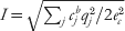$I \equals \sqrt {\sum\nolimits_{j} {c_{j}^{b} q_{j}^{\setnum{2}} \sol 2e_{c}^{\setnum{2}} } } $ is the ionic strength and e _c is the electron charge. The Debye–Hückel length is considered as a length scale below which mobile ions experience the ESP of the solute and interact with it.

Using the potential obtained by solving the PB equation, the electrostatic free energy can be obtained via a variety of integral formulations (Chen et al., 2010, Reference Chen, Baker and Wei2011b; Gilson, Reference Gilson1995; Holm et al., Reference Holm, Kekicheff and Podgornik2001; Micu et al., Reference Micu, Bagheri, Ilin, Scott and Pettitt1997; Sharp & Honig, Reference Sharp and Honig1990a). These free energy expressions arise both from physical considerations as well as from a purely mathematical standpoint. Statistical physics can derive the PB equation and its associated free energy from a saddle-point approximation of a more complicated description of the electrolyte system (Holm et al., Reference Holm, Kekicheff and Podgornik2001). Functional minimization of the resulting free energy gives rise directly to the PB equation. It is also possible to differentiate these integral formulations of the electrostatic energy with respect to atomic position in order to obtain the electrostatic (i.e. polar) solvation mean force on each atom (Gilson et al., Reference Gilson, Davis, Luty and Mccammon1993; Im, Reference Im1998; Wagoner & Baker, Reference Wagoner and Baker2004, Reference Wagoner and Baker2006).

While the PB equation may be solved analytically for very simple cases (e.g. flat plate with a single symmetrical electrolytes), analytical solutions of the PB equation are not available for biomolecules with realistic shapes and charge distributions. Therefore, a numerical method is a necessary tool for biomolecular electrostatics. After Warwicker and Watson (Warwicker & Watson, Reference Warwicker and Watson1982) first introduced numerical methods to solve the PB equation at the active site of an enzyme, many different numerical methods have been developed and are being modified. Most numerical methods for the PB equation depend on the discretization of computational domain/space (i.e. a distribution of points and their connections), which is critical to both accuracy and efficiency. These methods include finite differences (Baker et al., Reference Baker, Sept, Joseph, Holst and Mccammon2001b; Davis & McCammon, Reference Davis and Mccammon1989; Holst & Saied, Reference Holst and Saied1993, Reference Holst and Saied1995; Nicholls & Honig, Reference Nicholls and Honig1991), finite elements (Baker et al., Reference Baker, Holst and Wang2000, Reference Baker, Sept, Holst and Mccammon2001a; Cortis & Friesner, Reference Cortis and Friesner1997a, Reference Cortis and Friesnerb; Dyshlovenko, Reference Dyshlovenko2002; Holst et al., Reference Holst, Baker and Wang2000), and boundary elements (Bajaj et al., Reference Bajaj, Chen and Rand2011; Bordner & Huber, Reference Bordner and Huber2003; Boschitsch & Fenley, Reference Boschitsch and Fenley2004; Juffer et al., Reference Juffer, Botta, Vankeulen, Vanderploeg and Berendsen1991; Zauhar & Morgan, Reference Zauhar and Morgan1988).

Because of their simpler spatial discretization of the computational domain, finite differences have been the most popular numerical methods for the PB equation in bimolecular electrostatics. Finite difference-based PB solvers include APBS (Baker et al., Reference Baker, Sept, Joseph, Holst and Mccammon2001b), matched interface and boundary (MIB) (Chen et al., 2001; Yu & Wei, Reference Yu and Wei2007; Yu et al., Reference Yu, Geng and Wei2007a, Reference Yu, Zhou and Weib; Zhou & Wei, Reference Zhou and Wei2006), DelPhi (Klapper et al., Reference Klapper, Hagstrom, Fine, Sharp and Honig1986; Rocchia et al., Reference Rocchia, Sridharan, Nicholls, Alexov, Chiabrera and Honig2002), MEAD (Bashford, Reference Bashford, Ishikawa, Oldehoeft, Reynders and Tholburn1997), UHBD (Madura et al., Reference Madura, Briggs, Wade, Davis, Luty, Ilin, Antosiewicz, Gilson, Bagheri, Scott and Mccammon1995), ZAP (Grant et al., Reference Grant, Pickup and Nicholls2001), the PBEQ (Im, Reference Im1998) module in CHARMM (Brooks et al., Reference Brooks, Brooks, Mackerell, Nilsson, Petrella, Roux, Won, Archontis, Bartels, Boresch, Caflisch, Caves, Cui, Dinner, Feig, Fischer, Gao, Hodoscek, Im, Kuczera, Lazaridis, Ma, Ovchinnikov, Paci, Pastor, Post, Pu, Schaefer, Tidor, Venable, Woodcock, Wu, Yang, York and Karplus2009), and the PB solver in AMBER (Luo et al., Reference Luo, David and Gilson2002). The APBS solver provides scalable electrostatics by uniquely combing standard finite difference focusing techniques (Gilson & Honig, Reference Gilson and Honig1987) and the Bank–Holst algorithm (Bank & Holst, Reference Bank and Holst2003) into a parallel focusing method that allows solution of the PB equation for molecules of arbitrary size. A new MIB method (Chen et al., 2001; Geng & Wei, Reference Geng and Wei2001; Xia et al., Reference Xia, Zhan and Wei2011; Yu et al., Reference Yu, Geng and Wei2007a, Reference Yu, Zhou and Weib ; Zhou & Wei, Reference Zhou and Wei2006) implemented the analytical molecular surface in their interface method for solving the PB equation. This method was the first biomolecular PB solver enforcing the continuity conditions of both the ESP and its flux at the molecular surface. Wei et al. (Yu & Wei, Reference Yu and Wei2007; Yu et al., Reference Yu, Geng and Wei2007a, Reference Yu, Zhou and Weib) extended their work to further develop MIB-based PB solvers called MIBPB-II and MIBPB-III in order to accommodate geometric and charge singularities, respectively.

Finite-element methods provide more flexibility than finite differences by permitting adaptive mesh refinement in regions of high error. The local nature of this refinement, together with robust multilevel solvers (Holst, Reference Holst2001), provides unique multiscale capabilities. Significant finite-element work related to the PB equation was performed by Holst and co-workers (Baker et al., Reference Baker, Holst and Wang2000, Reference Baker, Sept, Holst and Mccammon2001a, Reference Baker, Sept, Joseph, Holst and Mccammonb; Holst, Reference Holst2001; Holst & Saied, Reference Holst and Saied1993, Reference Holst and Saied1995; Holst et al., Reference Holst, Baker and Wang2000). More recently, Chen et al. (Reference Chen, Holst and Xu2007a) have provided the first complete convergence result for a numerical discretization technique for the non-linear PB (NLPB) equation with delta distribution sources and introduced the first convergent adaptive method for the PB equation. Finite-element solutions are currently available through the FEtk solver (http://www.fetk.org/) with a biomolecular electrostatics interface provided APBS (http://www.poissonboltzmann.org/).

Boundary element methods (BEM) use Green's theorem to reformulate the linear PB equation as boundary integral equations (Allison, Reference Allison2001; Altman et al., Reference Altman, Bardhan, White and Tidor2009; Bajaj et al., Reference Bajaj, Chen and Rand2011; Bharadwaj et al., Reference Bharadwaj, Windemuth, Sridharan, Honig and Nicholls1995; Boschitsch & Fenley, Reference Boschitsch and Fenley2004; Boschitsch et al., Reference Boschitsch, Fenley and Zhou2002; Juffer et al., Reference Juffer, Botta, Vankeulen, Vanderploeg and Berendsen1991; Lu et al., Reference Lu, Cheng, Huang and Mccammon2010; Yoon & Lenhoff, Reference Yoon and Lenhoff1990; Zauhar, Reference Zauhar1995; Zauhar & Morgan, Reference Zauhar and Morgan1985, Reference Zauhar and Morgan1988; Zhou, Reference Zhou1993). Unlike finite differences and finite elements, the unknowns and domain discretization are only on a 2D surface rather than a 3D volume. For the NLPB equation, 3D volume integrals are involved in the integral equations, which reduce the efficiency of the methods, but still require a smaller number of unknowns than finite difference or finite-element methods. BEMs assume a discontinuous dielectric function at the molecular interface with the solvent; as such, they are suitable for a relatively narrow range of dielectric formulations. Advantages of BEM include (i) the reduction of the unknowns, (ii) exact treatment of boundary conditions at infinity, and (iii) explicit treatment of the physical interface conditions (continuity in potential and jump in its normal derivative). However, Green's functions are not available for the NLPB equation and the BEM may not be efficient because of numerous boundary integral operations and singular boundary integrals that can affect the accuracy and/or stability. Recently, a hybrid finite difference BEM approach was introduced to improve computational efficiency (Boschitsch & Fenley, Reference Boschitsch and Fenley2004). This approach is based on the separation of ESP into a linear component satisfying the linear PB equation and is solved using a fast BEM and a correction term accounting for non-linear effects and optionally, the presence of an ion-exclusion layer.

A completely different approach to solution of the linearized PB equation has been suggested by Mascagni and co-workers (Mascagni & Simonov, Reference Mascagni and Simonov2004; Simonov et al., Reference Simonov, Mascagni and Fenley2007). Their technique uses Monte Carlo methods that simulate random walks in the problem domain to solve the linear PB equation. This random walk approach is sufficiently flexible to work with complicated biomolecular geometries and can be used to calculate the molecular electrostatic properties for a series of salt concentration values simultaneously.

7.3 Simpler models for polar solvation

In addition to the PB model, simpler models have also been developed based on continuum electrostatics principles. These simple models include distance-dependent dielectric functions, analytic continuum methods (Schaefer & Karplus, Reference Schaefer and Karplus1996), the so-called Effective Energy Function (EEF) approach (Lazaridis & Karplus, Reference Lazaridis and Karplus1999) and the improved ABSINTH model (Vitalis & Pappu, Reference Vitalis and Pappu2009) and generalized Born (GB) models. The GB model is one of the most popular models and was developed by Still et al. in 1990 (Still et al., Reference Still, Tempczyk, Hawley and Hendrickson1990) and subsequently revised by several others (Anandakrishnan et al., Reference Anandakrishnan, Daga and Onufriev2011; Bashford & Case, Reference Bashford and Case2000; Brown & Case, Reference Brown and Case2006; Chen, Reference Chen2010; Chen et al., Reference Chen, Im and Brooks2006; Clark et al., Reference Clark, Meshkat and Wiseman2009; Dominy & Brooks, Reference Dominy and Brooks1999; Feig & Brooks, Reference Feig and Brooks2004; Feig et al., Reference Feig, Onufriev, Lee, Im, Case and Brooks2004, Reference Feig, Tanizaki and Sayadi2008; Gallicchio et al., Reference Gallicchio, Zhang and Levy2002, Reference Gallicchio, Paris and Levy2009; Grant et al., Reference Grant, Pickup, Sykes, Kitchen and Nicholls2007; Grycuk, Reference Grycuk2003; Im et al., Reference Im, Lee and Brooks2003b; Jorgensen et al., Reference Jorgensen, Ulmschneider and Rives2004; Labute, Reference Labute2008; Lee et al., Reference Lee, Salsbury and Brooks2002; Onufriev et al., Reference Onufriev, Bashford and Case2000, Reference Onufriev, Case and Bashford2002; Osapay et al., Reference Osapay, Young, Bashford, Brooks and Case1996; Tjong & Zhou, Reference Tjong and Zhou2007b; Tsui & Case, Reference Tsui and Case2000; Xu et al., Reference Xu, Cheng and Yang2011; Zhu et al., Reference Zhu, Alexov and Honig2005). The GB model describes the solvent as a continuum medium, similar to the PB model, but provides a faster calculation of solvation energies and forces. The model is an approximation to the Poisson equation energy; it models a solute particle as a sphere whose internal dielectric permittivity coefficient is different from that of the external solvent. Specifically, it uses the analytical solvation energy resulting from the solution of the Poisson equation for a simple sphere (Born, Reference Born1920).

Analytical solutions to electrostatic problems associated with various simple dielectric boundary conditions are discussed in many textbooks (Bottcher, Reference Bottcher1952; Jackson, Reference Jackson1975). A simple electrostatic model of a biomolecule in solution is a cavity with a charge distribution embedded in a high-dielectric continuum medium. The problem can be further simplified by considering a spherical cavity within which electrostatic interactions are calculated explicitly. By Gauss’ Law, the ESP outside the sphere is given by the usual Coulomb formula. However, since electric charges within the cavity polarize the high-dielectric medium, the total electric potential inside the cavity includes this effect as well as the direct Coulomb interactions between charges within the cavity. The electric potential associated with the polarization is called the ‘reaction field (RF)’ potential and can be represented by a summation of Legendre polynomials (Kirkwood, Reference Kirkwood1934) or by the Coulomb potential associated with image charges outside the cavity.

The image charge approach is usually formulated when the dielectric constant of medium is much larger than that of the cavity, the RF potential inside the cavity is approximately (Deng & Cai, Reference Deng and Cai2007; Friedman, Reference Friedman1975)

$${\rm \rmPhi }_{{\rm RF}} \lpar r\rpar \equals \mathop \sum \limits_{i \equals \setnum{1}}^{N} {{q_{i} \prime} \over {\varepsilon _{in} \vert {\underline r} \minus {\underline r}_{i} \prime \vert }}\comma $$

$$q_{i}{\prime} \equals {{\varepsilon _{in} \minus \varepsilon _{o} } \over {\varepsilon _{in} \plus \varepsilon _{o} }}{R \over {r_{i} }}q_{i} \comma $$

$${\underline r}_{i}{\prime} \equals \left( {R\sol {r}_{i} } \right)^{\setnum{2}} {\underline r}_{i} \comma $$

where q′ is the image charge that will interact with the solute and r′ is the location of the image charge outside the cavity. The total energy of the system, including both the gas-phase interaction energy of source charges and the RF energy, becomes (Wang & Hermans, Reference Wang and Hermans1995):

$$U \equals {1 \over 2}\mathop \sum \limits_{i \equals \setnum{1}}^{N} \mathop \sum \limits_{j \equals \setnum{1}}^{N} {{q_{i} q_{j} } \over {\varepsilon _{in} \vert {\underline r}_{i} \minus {\underline r}_{j} \vert }} \plus {1 \over 2}\mathop \sum \limits_{i \equals \setnum{1}}^{N} \mathop \sum \limits_{j \equals \setnum{1}}^{N} {{q_{i} q_{j} \prime} \over {\varepsilon _{in} \vert {\underline r}_{i} \minus {\underline r}_{j} \prime\vert }}\comma $$

where the sums implicitly exclude self-interactions for i = j. The first term of this energy expression indicates the direct electrostatic interactions between source charges in the cavity, whereas the second term includes the RF effect through the interactions between the source charges and image charges. Note that the second term includes not only the interaction between each source charge with the image charges of other source charges but also that between each source charge with its own image charge. By placing solute molecules in a spherical water droplet, Wang & Hermans (Reference Wang and Hermans1995) adapted the Friedman's image charge method in molecular dynamic simulations to account for the dielectric effect outside the simulated sphere. Deng & Cai (Reference Deng and Cai2007) showed that Friedman's formula is the zeroth-order term in the Kirkwood series expansion with respect to ∊_in/∊_o. It is also noted that Friedman's approximation is inconsistent with Born formula when all the charges are located at the center of the spherical cavity. Based on the work by Neumann (Neumann, Reference Neumann1883), a multiple image of charge method was proposed whereby the single image charge is replaced by a charge distribution extending from the image charge position to infinity in the radial direction (Lindell, Reference Lindell1992; Norris, Reference Norris1995). An efficient fast multipole algorithm was developed to take advantage of the accuracy of the multiple image method while making it computational tractable for simulation purposes (Cai et al., Reference Cai, Deng and Jacobs2007; Deng & Cai, Reference Deng and Cai2007).

The Legendre polynomial solution of the spherical system was given by Kirkwood in 1934 (Kirkwood, Reference Kirkwood1934). For a system with a set of point charges q_k in a spherical cavity of radius a, the RF potential at r inside the sphere is given by

$$V\lpar r\rpar \equals {1 \over {\varepsilon _{in} }}\mathop \sum \limits_{l \equals \setnum{0}}^{\infty } {{\lpar l \plus 1\rpar \lpar \varepsilon _{in} \minus \varepsilon _{o} \rpar } \over {\lpar n \plus 1\rpar \varepsilon _{o} \plus n\varepsilon _{in} }}{{r^{l} } \over {a^{\setnum{2}l \plus \setnum{1}} }}\mathop \sum \limits_{k \equals \setnum{1}}^{N} q_{k} r_{k}^{l} P_{l} \lpar {\rm cos}\,\theta \rpar .$$

In the equation above, the dielectric constants inside the spherical cavity is ∊_in. The terms q_k r_k^l (l = 0, 1, 2, …) are the multipole moments of the charge distribution inside the sphere. The expansion reduces to the Born (Born, Reference Born1920) or Onsager (Onsager, Reference Onsager1936) approximation in the special case of a single ion or dipole buried at the center of the spherical cavity.

With growing interests in sophisticated electrostatic models involving point multipoles and electronic polarization, the Kirkwood's RF theory has been extended beyond partial charges. Orttung generalized the Kirkwood–Westheimer model (Kirkwood, Reference Kirkwood1938) for different shapes, charges, and polarizabilities (Orttung, Reference Orttung1978). Warshel developed a multiscale model to describe the interactions among explicit solute (point charge), immediate solvation shell (point dipole) and the surrounding continuum (RF) (Warshel, Reference Warshel1979). Felder and Applequist introduced inducible dipoles to represent the solute electrostatics and derived the corresponding RF expressions for spherical and ellipsoidal cavities (Felder & Applequist, Reference Felder and Applequist1981). Kong and Ponder obtained the RF energy and force for arbitrary point multipole distributions located off the center of the spherical cavity (Kong, Reference Kong1997). Nymand and Linse developed a RF model for solutes of point charges, dipoles and polarizabilities (Nymand & Linse, Reference Nymand and Linse2000). Recently, Schnieders and Ponder introduced generalized Kirkwood (GK) model to eliminate the partial charge restriction inherent to GB analytic continuum electrostatics (Schnieders & Ponder, Reference Schnieders and Ponder2007). GK defines a self-consistent RF for solutes modeled by polarizable atomic multipoles, which are not only more accurate and transferable than partial charges but also more expensive. Davis developed an inducible multipole solvation model that exhibits an exact series representation of the external electrostatic field for a collection of dielectric cavities with centrosymetric internal charge distributions and arbitrary external charge distributions (Davis, Reference Davis1994). Fenley et al. (Reference Fenley, Gordon and Onufriev2008) derived a closed-form analytical approximation to the Poisson equation for an arbitrary distribution of point charges and a spherical dielectric boundary. Their simple, parameter-free formula was obtained from the Kirkwood solution by an approximate summation method and presents continuous ESP everywhere in space.

The GB model can be thought of as a good analytical approximation to the analytical models described above. In particular, it uses the analytical solvation energy resulting from the solution of the Poisson equation for a simple sphere and needs a much lower computational cost, compared to solving the PB equation. Using the GB model, the electrostatic solvation-free energy can be approximated by a modified form of the analytical solvation energy for a sphere (Still et al., Reference Still, Tempczyk, Hawley and Hendrickson1990):

$$G_{el} \cong \minus {1 \over 2}\left( {1 \minus {1 \over {\varepsilon _{{\rm sol}} }}} \right)\mathop \sum \limits_{i\comma j} {{Q_{i} Q_{j} } \over {f_{ij}^{{\rm GB}} }}\comma $$

where f _ij^GB denotes the effective Born radii (when i=j) and the effective interaction distance (when i≠j), respectively. The most common form given by Still et al. (Reference Still, Tempczyk, Hawley and Hendrickson1990) is

$$f_{ij}^{{\rm GB}} \equals \left[ {r_{ij}^{\setnum{2}} \plus R_{i} R_{j} {\rm exp}\left( { \minus {{r_{ij}^{\setnum{2}} } \over {4R_{i} R_{j} }}} \right)} \right]^{\setnum{1}\sol \setnum{2}} \comma $$

whereR_i are the effective radii of the atoms and r_ij are the distance between atoms i and j. It is essential to calculate the effective radii of the atoms efficiently and accurately. A previous study (Onufriev et al., Reference Onufriev, Case and Bashford2002) demonstrated that the GB model can provide comparable results to the Poisson equation when one uses perfect GB radii that reproduce the atoms’ self-energies as obtained from the Poisson equation. This observation implies that an accurate estimation of the radii is critical for reliability of the GB model. Many studies have been performed to improve the GB model not only with general corrections (Mongan et al., Reference Mongan, Simmerling, Mccammon, Case and Onufriev2007) but also with revised formulations aiming at biomacromolecules such as proteins and nucleic acids (Dominy & Brooks, Reference Dominy and Brooks1999; Onufriev et al., Reference Onufriev, Bashford and Case2000; Sigalov et al., Reference Sigalov, Fenley and Onufriev2006) and biological membranes (Im et al., Reference Im, Feig and Brooks2003a; Tanizaki & Feig, Reference Tanizaki and Feig2005). The GB model has also been extended to provide approximations to the full NLPB equation because of its computational benefit (Tjong & Zhou, Reference Tjong and Zhou2007a, Reference Tjong and Zhou2007b).

7.4 Continuum models for non-polar solvation

The low-detail continuum polar solvation models above are generally decoupled from the non-polar energetics of the system. Therefore, non-polar contributions must be added into the system to complement the polar energetics. The importance of non-polar solvation is well known, but has often been treated with a very simple approximation that assumes non-polar energy is proportional to solvent-accessible area (Chothia, Reference Chothia1974; Massova & Kollman, Reference Massova and Kollman2000; Sharp et al., Reference Sharp, Nicholls, Fine and Honig1991a, Reference Sharp, Nicholls, Friedman and Honigb; Wesson & Eisenberg, Reference Wesson and Eisenberg1992)

$$G_{{\rm non{\hbox{-}}polar}} \lpar \hskip1pt\vec{x}\hskip1.3pt\rpar \cong \gamma A\lpar \hskip1pt\vec{x}\hskip1.3pt\rpar .$$

This approximation is motivated by the solvation area of linear alkanes in water. Here γ is a microscopic solvent surface tension parameter (not a macroscopic surface tension of solvent) which can be chosen to reproduce the solvation free energy of non-polar molecules (Sharp et al., Reference Sharp, Nicholls, Fine and Honig1991a, Reference Sharp, Nicholls, Friedman and Honig1991b; Simonson & Brunger, Reference Simonson and Brunger1994; Sitkoff et al., Reference Sitkoff, Sharp and Honig1994b), including model side chain analogs (Wesson & Eisenberg, Reference Wesson and Eisenberg1992; Wimley et al., Reference Wimley, Creamer and White1996). The surface tension parameter can be modeled as a single universal value used for all atoms or different values may be assigned for each atom type. While the simplest description has been successful, it has several caveats, including the difficulty of rationalizing surface tension parameter values (Chothia, Reference Chothia1974; Eisenberg & McLachlan, Reference Eisenberg and Mclachlan1986; Sharp et al., Reference Sharp, Nicholls, Fine and Honig1991a, Reference Sharp, Nicholls, Friedman and Honig1991b; Sitkoff et al., Reference Sitkoff, Sharp and Honig1994b) as well as inaccurate descriptions of detailed aspects of non-polar solvation energies (Gallicchio & Levy, Reference Gallicchio and Levy2004), peptide conformations (Su & Gallicchio, Reference Su and Gallicchio2004), and non-polar solvation forces (Wagoner & Baker, Reference Wagoner and Baker2006).

Recent work (Gallicchio et al., Reference Gallicchio, Kubo and Levy2000; Gallicchio & Levy, Reference Gallicchio and Levy2004; Levy et al., Reference Levy, Zhang, Gallicchio and Felts2003; Wagoner & Baker, Reference Wagoner and Baker2006) has built upon a significant amount of existing research into non-polar effects (Ashbaugh, Reference Ashbaugh2009; Ashbaugh & Pratt, Reference Ashbaugh and Pratt2006; Ben-Naim, Reference Ben-Naim2006; Chandler, Reference Chandler2005; Gu et al., Reference Gu, Rahi and Helms2004; Huang & Chandler, Reference Huang and Chandler2002; Huang et al., Reference Huang, Geissler and Chandler2001; Hummer, Reference Hummer1999; Hummer & Garde, Reference Hummer and Garde1998; Hummer et al., Reference Hummer, Garde, García, Pohorille and Pratt1996, Reference Hummer, Garde, Garcia and Pratt2000; Pitera & van Gunsteren, Reference Pitera and Van Gunsteren2001; Pratt, Reference Pratt2002; Pratt & Chandler, Reference Pratt and Chandler1977; Pratt & Pohorille, Reference Pratt and Pohorille1992, Reference Pratt and Pohorille2002; Rajamani et al., Reference Rajamani, Truskett and Garde2005; Tan et al., Reference Tan, Tan and Luo2007) to develop computationally efficient, but more energetically complete, models for non-polar solvation energy that include important attractive van der Waals interactions between solvent and solute (Gallicchio & Levy, Reference Gallicchio and Levy2004; Gallicchio et al., Reference Gallicchio, Kubo and Levy2000, Reference Gallicchio, Zhang and Levy2002; Wagoner & Baker, Reference Wagoner and Baker2006) and repulsive solvent-accessible volume terms (Wagoner & Baker, Reference Wagoner and Baker2006). For example, Wagoner and Baker proposed a non-polar solvation model based on the free energy functional (Wagoner & Baker, Reference Wagoner and Baker2006):

$$G_{{\rm non{\hbox{-}}polar}} \lpar \hskip1pt\vec{x}\hskip1pt\rpar \cong \gamma A\lpar \vec{x}\hskip1.3pt\rpar \plus pV\lpar \vec{x}\hskip1.3pt\rpar \plus \bar{\rho }\mathop \sum \limits_{i \equals \setnum{1}}^{N} \int\limits_{\rm \rmOmega } {u_{i}^{{\rm att}} \lpar \vec{x}_{i} \comma \, \vec{y}\rpar \theta \lpar \vec{x}\comma \, \vec{y}\rpar \ {\rm d}\vec{y}} \comma $$

where p is a solvent hydrodynamic pressure parameter, V is a solvent accessible volume, and $\bar{\rho }$ is the bulk solvent density. Here Ω denotes the solvent accessible region outside the solute, $u_{i}^{{\rm att}} \lpar \vec{x}_{i} \comma \, \vec{y}\hskip2.3pt\rpar $ is the attractive component of the non-polar interaction potential (for atom i) between a solute in conformation $\vec{x}$ and solvent at position $\vec{y}$, and $\theta \lpar \vec{x}\comma \,\vec{y}\hskip1.3pt\rpar $ is a characteristic function defined as a product of per-atom characteristic functions θ_i. This model showed very good agreement with explicit solvent results, which suggests that the addition of appropriate dispersion and volume terms is essential to describe atomic scale non-polar forces.

Recent studies on the solvation of atomistic and nanoscale solutes reveal that a coupling exists between the hydrophobic, dispersion, and electrostatic contributions to the solvation-free energy. The fact that the effective location of the solvent–solute interface can rely on the local electrostatic and dispersive (Huang & Chandler, Reference Huang and Chandler2002) potentials suggests that such polar and non-polar components should be coupled in implicit solvent models. For example, Ashbaugh & Paulaitis (Reference Ashbaugh and Paulaitis1998) pointed out that a correct balance between non-polar and polar (or electrostatic) contributions is critical in their study of amphiphiles. To take into account polar–non-polar coupling, Dzubiella et al. (Reference Dzubiella, Swanson and Mccammon2006a, Reference Dzubiella, Swanson and Mccammonb) proposed a theoretical formalism based on the minimization of the Gibbs-free energy of the solvent with respect to a solvent volume exclusion function. Unlike existing implicit solvent approaches, the solvent–solute interface is an output of the model. Therefore, the coupling is indeed implemented by the geometrical description of capillary interfaces. The formalism captures the sensitivity of hydration to the particular form of the solute–solvent interactions in agreement with recent computer simulations. More recently, as discussed above, Wei, Baker, and Chen have combined the non-polar free energy functional introduced above with the PB polar solvation free energy functional for a self-consistent description of solvation and biomolecular surfaces (Chen et al., Reference Chen, Baker and Wei2010, Reference Chen, Baker and Wei2011b).

8.1 Quasi-chemical theory

Many solute–solvent interactions, typically short-ranged and structurally specific, can be characterized as chemical associations. Therefore, it is feasible to identify an inner shell around the solute that will accommodate strongly associating solvent molecules, and an outer shell that corresponds to the rest of the system, so that these regions can be treated with high-detail and low-detail models, respectively (Pratt & Laviolette, Reference Pratt and Laviolette1998; Pratt et al., Reference Pratt, Laviolette, Gomez and Gentile2001). Quasi-chemical theory provides a framework for such decomposition. The solvation free energy of Li⁺, Na⁺, K⁺, Zn²⁺, and other alkaline divalent metal cations in water have been successfully predicted on the basis of quasi-chemical theory and ab initio molecular dynamics and provided good agreement with experiment (Asthagiri et al., Reference Asthagiri, Pratt, Paulaitis and Rempe2004; Rempe et al., Reference Rempe, Asthagiri and Pratt2004). The quasi-chemical method can provide a level of accuracy comparable to that reported in QM, but it is far less expensive than the standard QM/MM method. However, this method still has several limitations, including difficulty treating strongly disordered solvation shells and heterogeneous environments.

8.2 Implicit–explicit solvation models

Over the years, a number of generalized RF methods have been implemented in molecular simulations based on the continuum Kirkwood expansion (Tironi et al., Reference Tironi, Sperb, Smith and Gunsteren1995) with a variety of applications in explicit solvent molecular simulation methodology (Alper & Levy, Reference Alper and Levy1993; Baker et al., Reference Baker, Hünenberger and Mccammon1999; Beglov & Roux, Reference Beglov and Roux1994; Brooks, Reference Brooks1985, Reference Brooks1987; Hünenberger & Gunsteren, Reference Hünenberger and Gunsteren1998; Lau et al., Reference Lau, Alper, Thacher and Stouch1994; Schreiber & Steinhauser, Reference Schreiber and Steinhauser1992a, Reference Schreiber and Steinhauserb; Steinbach & Brooks, Reference Steinbach and Brooks1994; Tironi et al., Reference Tironi, Sperb, Smith and Gunsteren1995). However, such RF methods also have a natural application to hybrid models. One such example is the general solvent boundary potential (GSBP), where a sphere contains an explicit solvent region while reaction influence of the surrounding environment is represented by a continuum model (Im et al., Reference Im, Berneche and Roux2001). The generalized solvent boundary model has been applied to the calculation of protein–ligand binding free energy (Banavali et al., Reference Banavali, Im and Roux2002; Deng & Roux, Reference Deng and Roux2008) and recently extended to QM/MM settings (Schaefer et al., Reference Schaefer, Riccardi and Cui2005).

Lee et al. (Reference Lee, Salsbury and Olson2004) developed a hybrid solvation scheme to incorporate a continuum RF via GB theory and use a generalized sum-over-spheres boundary, where water molecules are constrained with respect to their closet solute atom location. The hybrid method was first tested on single ion and protein L simulations; and the results achieved similar equilibrium and dynamical observables as the conventional explicit solvent simulations except for some deviations near the boundaries. The hybrid solvent model combined with replica exchange molecular dynamics has been used to study the free energy of formation of ion pairs using model peptides. This work suggested that the structure of salt bridge in explicit solvent can be reproduced by the hybrid solvent approach, but not by GB alone (Okur et al., Reference Okur, Wickstrom, Layten, Geney, Song, Hornak and Simmerling2006, Reference Okur, Wickstrom and Simmerling2008).

An important long-standing difficulty of mixed resolution solvent models is structural artifacts near the explicit–implicit solvent boundary. A promising approach to solve this challenging problem is the smoothly decoupled particle interface (SDPI) described recently by Wagoner and Pande (Wagoner & Pande, Reference Wagoner and Pande2011), which introduces a third, buffering shell between an inner region of explicit solvent and an outer continuum solvent. The function of the buffering shell is to transition smoothly the explicit particle density between that of the innermost region to zero at the interface with the outer continuum.

8.3 Particle-based continuum models

An interesting particle-based macroscopic solvent model, which represents electronic and oriental polarization of water molecules by an ensemble of polarizable pseudo-particles (PPP) (Basdevant et al., Reference Basdevant, Borgis and Ha-Duong2004, Reference Basdevant, Ha-Duong and Borgis2006) in a framework that bears some similarity to the polarizable Langevin dipoles of Warshel (Papazyan & Warshel, Reference Papazyan and Warshel1997, Reference Papazyan and Warshel1998) has recently been proposed. In this approach, the solute electric field induces dipoles at the centers of the solvent PPPs which, in turn, interact with the solute charge distribution. However, the solvent PPPs only interact with each other through the van der Waals interactions. The theoretical foundation is built upon on Marcus’ functional for solvation free energy (Marcus, Reference Marcus1956). The functional is minimized to the equilibrium condition following the Coulomb field approximation and a localized, off-lattice Langevin dipole approach (Florián & Warshel, Reference Florián and Warshel1997) in which the solvent–solvent polarization is ignored (HaDuong et al., Reference Haduong, Phan, Marchi and Borgis2002). This novel approach has the potential to bridge the gap between implicit and explicit solvent-based solvent methods. The PPP is computationally more efficient than explicit solvent methods as it produces the macroscopic dielectric response instantaneously. However, unlike implicit solvent methods, it aims to directly capture non-polar influences via solvent–solute van der Waals interactions without resorting to additional approximations. While this method shows lower computational cost than explicit models and can be extended to coarse-grained solutes (Basdevant et al., Reference Basdevant, Borgis and Ha-Duong2007; Ha-Duong et al., Reference Ha-Duong, Basdevant and Borgis2009), the parameterization of the model is complicated, involving empirically scaling the van der Waals radius based on the Born energy of ions and charges of solute atoms to match Kirkwood solvation energy of a spherical cavity.