1 Introduction
The displacement of viscous fluids by less viscous ones in porous media often leads to the development of instabilities. These instabilities known as viscous fingering have been first analysed by Hill (Reference Hill1952) and Slobod & Caudlel (Reference Slobod and Caudlel1952) and the physical dynamics was explained by Saffman & Taylor (Reference Saffman and Taylor1958). Numerous subsequent studies have examined the instability both in the case of miscible (Tan & Homsy Reference Tan and Homsy1986, Reference Tan and Homsy1987, Reference Tan and Homsy1992; Ruith & Meiburg Reference Ruith and Meiburg2000), immiscible (Paterson Reference Paterson1981; Kueper & Frind Reference Kueper and Frind1988; Zheng, Kim & Stone Reference Zheng, Kim and Stone2015) and partially miscible flows (Huang & Chen Reference Huang and Chen2015). Extensive reviews on this topic have been presented by Homsy (Reference Homsy1987), Yortsos (Reference Yortsos1990) and McCloud & Maher (Reference McCloud and Maher1995).
Studies on viscous fingering in immiscible displacements have investigated the effects of the main flow parameters, namely the viscosity ratio, the surface tension and the injection rate, and how they affect the development of fingers and their morphology. Most of the studies adopted the Hele-Shaw (HS) cell flow geometry as it is analogous to a homogeneous porous medium. Bataille (Reference Bataille1968) and later Paterson (Reference Paterson1981) developed expressions that relate the growth rate of instabilities in the early stages of the flow to the governing parameters for immiscible displacements in a radial HS cell. Experiments involving the injection of dyed oil into glycerine in a radial HS cell showed that stronger injection rates result in an enhancement of viscous fingering (Chen Reference Chen1987). The effects of surface tension were discussed to some extent by Cardoso & Woods (Reference Cardoso and Woods1995), showing its stabilizing effect on the interface to be important mainly when the radius of the injected fluid is small. Hornof & Baig (Reference Hornof and Baig1995) studied the effects of the viscosity of oil being displaced by water in a quarter of a five spot HS cell, and observed that the oil recovery is inversely proportional to the viscosity of oil.
The vast majority of existing studies have focused on displacements under constant injection. There are however numerous practical processes where the injection is actually time dependent. These include the use of time-dependent feed strategies in trickle-bed reactors to ensure flow uniformity and avoid hot spot formation as well as enhanced oil recovery processes such as cyclic steam stimulation processes (see Barrio et al. Reference Barrio, Schaub, Rohde, Rabe, Vogel, Cambra, Arias and Gemez2007; Al-Gosayir et al. Reference Al-Gosayir, Leung, Babadagli and Al-Bahlani2013).
Surguchev et al. (Reference Surguchev, Koundin, Melberg, Rolfsvg and Menardr2002) modelled numerically the application of cyclic waterflooding in heterogeneous oil reservoirs, and showed that better recovery can be achieved through time-dependent injection schemes in comparison with constant injection ones. The effects of oscillation in the injection pressure at different frequencies were examined by Gland & Pisarenko (Reference Gland, Pisarenko and Kümpel2003). The authors used air to displace oil in a radial HS cell, and concluded that the oscillations led to an attenuation of the instability. It was reported that due to the pressure oscillation there appears to be a ‘stiffening’ of the interface which resulted in less fingering. In another study by Brailovsky et al. (Reference Brailovsky, Babchin, Frankel and Sivashinsky2006), numerical simulations of flows in a radial HS cell revealed that displacement schemes that involve injection periods followed by long times of no injection result in the contraction of fingers due to the stabilizing effects of surface tension. A subsequent nonlinear simulation study for radial HS cells by Li et al. (Reference Li, Lowengrub, Fontana and Palffy-Muhoray2009) analysed the finger’s morphology and structures for injection flows that vary like
 $t^{-1/3}$
. It was found that different limiting shapes, which correspond to a structure that an interface maintains after a long time, are dependent on the magnitude of the injection rate. Different magnitudes of injection rates would therefore lead to peculiar symmetrical shapes, regardless of the initial shape of the interface. Using the same time-dependent injection scheme, Leshchine et al. (Reference Leshchine, Thrasher, Mineev-Weinstein and Swinney2010) evaluated the growth of the interface and were able to estimate the surface tension using the harmonics of the interface.
Dias, Parisio & Miranda (Reference Dias, Parisio and Miranda2010) used linear stability analysis to examine the onset of instabilities of flow displacements in a radial HS cell, and proposed the adoption of piecewise injection policies as an effective way for reducing the size of instabilities. A related study by Dias & Miranda (Reference Dias and Miranda2010) showed that the application of injection rates that vary according to
 $t^{-1/3}$
are able to considerably attenuate the branching of fingers in a radial HS cell at the onset of the nonlinear regime. In a subsequent analysis, dos Reis & Miranda (Reference dos Reis and Miranda2011) attempted to control viscous fingering instabilities in different types of Hele-Shaw cell geometry, namely with conical and spherical shapes, and reported expressions for time-dependent injection rates based on linear stability analysis. Results from another study by Dias et al. (Reference Dias, Alvarez-Lacalle, Carvalho and Miranda2012) indicated that a specific type of monotonic injection scheme is capable of attenuating instabilities in radial immiscible displacements more than any other injection policy in the linear regime. In a related work, Dias & Miranda (Reference Dias and Miranda2013) investigated the occurrence of perturbation in crystal growth, and observed that the same linear policy was able to reduce interfacial deformities. A subsequent related study was carried out by Huang & Chen (Reference Huang and Chen2015) who have used full nonlinear simulations in a radial HS cell to analyse the flow development while also expanding the analysis to different degrees of fluids miscibility. It was confirmed that the linear injection scheme proposed by Dias et al. (Reference Dias, Alvarez-Lacalle, Carvalho and Miranda2012) does indeed attenuate the instability in immiscible displacements, but interestingly the same injection scheme actually leads to an enhancement of the instabilities in the case of miscible displacements. The authors were able to establish their conclusions quantitatively by tracking the distance of the inward fingers and of the outward fingers in time.
A series of nonlinear simulations studies dealing with time-dependent miscible flow displacements in rectilinear geometries were carried out by Yuan & Azaiez (Reference Yuan and Azaiez2014) and Yuan & Azaiez (Reference Yuan and Azaiez2015). In particular, reactive flow displacements under periodic stepwise injection schemes were analysed (Yuan & Azaiez Reference Yuan and Azaiez2014). It was reported that displacements that would be stable under a constant injection flow can become unstable under time-dependent injection schemes. The resulting unstable flows lead to more complex finger morphologies and a greater extent of reactivity as a result of the solutions enhanced mixing. The effects of inertia in cyclic time-dependent injections were considered and it was found that instabilities may vary non-monotonically with respect to the period and amplitude of the injection cycle (Yuan & Azaiez Reference Yuan and Azaiez2015). A recent study by Chen et al. (Reference Chen, Huang, Huang and Miranda2015) observed that one way to enhance mixing in a radial HS cell between two miscible fluids is by injecting high and low viscosity fluid sequentially under increasingly small time intervals for each injection.
A more comprehensive investigation of time-dependent injection schemes for immiscible flows was recently presented by Lins & Azaiez (Reference Lins and Azaiez2016). The effects of monotonic and cyclic injection schemes were compared, and it was found that modifying the period and amplitude of the cycles can be used as a tool to reduce the extent of instabilities. Modifying the injection policy, however, had limited impact as the flow became more prone to viscous fingering. A novel control scheme where the injection rate is dependent on the strength of the interfacial instability was proposed and was shown to be capable of reducing the size of fingers and the extent of their growth.
Based on the results reported in existing studies that dealt with time-dependent injections, it is clear that the interfacial instability is strongly dependent on the injection policy, and there is a potential for using judiciously the injection flow parameters to control the fate of the flow. The objective of the present study is to analyse thoroughly the effects of the period of the injection schemes on the fingers structures and morphology. Unlike most of the previous studies that were either based exclusively on linear stability analysis of immiscible/miscible flows, or nonlinear simulations of miscible flows in rectilinear geometries, the present study will examine the nonlinear development of the fingering instability for immiscible flows under radial displacement. The displacements are analysed in detail under oscillatory flow to determine the effects of the period of the injection. In this process it will be shown that the flow dynamics actually depends in a nonlinear fashion on the period and exhibit a resonance-like behaviour that depends on the fluids physical properties.
2 Model and governing equations
In this study, immiscible displacements in porous media under cyclic injection schemes are investigated. The two-dimensional flow develops radially in the porous medium which is assumed to be homogeneous with constant permeability
 $K$
. A fluid of viscosity
 $\unicode[STIX]{x1D707}_{1}$
is injected into the porous medium containing another fluid of viscosity
 $\unicode[STIX]{x1D707}_{2}$
, where
 $\unicode[STIX]{x1D707}_{2}/\unicode[STIX]{x1D707}_{1}$
is always larger than 1. A related parameter that will be used in the remaining of this study is the mobility
 $\unicode[STIX]{x1D6FD}=K/\unicode[STIX]{x1D707}$
; defined as the ratio of the medium permeability and the fluid viscosity. The surface tension between the two fluids is denoted by
 $\unicode[STIX]{x1D70E}$
.
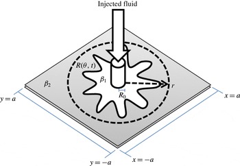
Schematic of a radial displacement in a porous medium.

The position of the interface is defined by the function
 $R(\unicode[STIX]{x1D703},t)$
, which is specified with respect to the angular position of the interface
 $\unicode[STIX]{x1D703}$
and the time
 $t$
after which injection begins. The problem is solved in a
 $[2a\times 2a]$
square domain with the origin at the centre of the domain. The domain size is chosen large enough for the interface to expand before breakthrough. An illustration of the domain is shown in figure 1. The problem is initialized by setting a circular interface between the two fluids with a radius equal to
 $R_{0}$
. This core radius
 $R_{0}$
defines the region where fluid injection takes place, and coincides with the initial radius of the interface;
 $R(\unicode[STIX]{x1D703},t=0)=R_{0}$
.
The model equations that govern the flow are:
 $$\begin{eqnarray}\displaystyle & \displaystyle \unicode[STIX]{x1D735}p=\left\{\begin{array}{@{}ll@{}}-\boldsymbol{U}/\unicode[STIX]{x1D6FD}_{1} & \text{fluid 1}\\ -\boldsymbol{U}/\unicode[STIX]{x1D6FD}_{2} & \text{fluid 2},\end{array}\right. & \displaystyle\end{eqnarray}$$
 $$\begin{eqnarray}\displaystyle & \displaystyle \unicode[STIX]{x1D735}\boldsymbol{\cdot }\boldsymbol{U}=\unicode[STIX]{x1D719}. & \displaystyle\end{eqnarray}$$
Equation (2.1) is Darcy’s law, where
 $\boldsymbol{U}$
is the velocity and
 $p$
the pressure while (2.2) represents the continuity equation with a source term
 $\unicode[STIX]{x1D719}$
.
In a constant injection displacement, the source
 $\unicode[STIX]{x1D719}(r)$
accounts for the injection of the higher mobility
 $(\unicode[STIX]{x1D6FD}_{1})$
fluid into the medium containing the lower mobility
 $(\unicode[STIX]{x1D6FD}_{2})$
fluid and is related to the total constant injection rate,
 $Q$
, according to (2.7),
 $$\begin{eqnarray}Q=\int _{0}^{2\unicode[STIX]{x03C0}}\int _{0}^{R_{0}}\unicode[STIX]{x1D719}(r)r\,\text{d}r\,\text{d}\unicode[STIX]{x1D703}.\end{eqnarray}$$
The source term
 $\unicode[STIX]{x1D719}$
, which is an approximation of the Dirac delta function across an area defined by a radius
 $R_{0}$
, is defined as follows (Peskin Reference Peskin1977; Hou et al.
Reference Hou, Li, Osher and Zhao1997; Ahmadlouydarab, Azaiez & Chen Reference Ahmadlouydarab, Azaiez and Chen2015):
 $$\begin{eqnarray}\unicode[STIX]{x1D719}(r)=\left\{\begin{array}{@{}ll@{}}\unicode[STIX]{x1D711}_{0}[1+\cos (\unicode[STIX]{x03C0}r/R_{0})], & r\leqslant R_{0}\\ 0, & r>R_{0}.\end{array}\right.\end{eqnarray}$$
In the above equations
 $r$
is the radial coordinate and
 $\unicode[STIX]{x1D711}_{0}$
is the injection strength coefficient.
For the case of a constant injection, the total flow rate is:
 $$\begin{eqnarray}Q=\unicode[STIX]{x1D711}_{0}R_{0}^{2}(\unicode[STIX]{x03C0}-4/\unicode[STIX]{x03C0})=\unicode[STIX]{x03C0}\unicode[STIX]{x1D719}_{0}R_{0}^{2},\end{eqnarray}$$
where
 $\unicode[STIX]{x1D719}_{0}$
refers to the constant injection rate divided by the core area and is related to
 $\unicode[STIX]{x1D711}_{0}$
;
 $\unicode[STIX]{x1D719}_{0}=\unicode[STIX]{x1D711}_{0}(1-4/\unicode[STIX]{x03C0}^{2})$
, which is divided by a factor of
 $1/2\unicode[STIX]{x03C0}R_{0}^{2}$
for all results with time-dependent injection processes.
In the present study we are interested in analysing time-dependent flow displacements that are based on a sinusoidal scheme of unit amplitude and period
 $T$
. To this end, the time-dependent source term
 $\unicode[STIX]{x1D719}(r,t)$
is defined as:
 $$\begin{eqnarray}\unicode[STIX]{x1D719}(r,t)=\left\{\begin{array}{@{}ll@{}}\unicode[STIX]{x1D711}_{0}[1+\cos (\unicode[STIX]{x03C0}r/R_{0})][1+\sin (2\unicode[STIX]{x03C0}t/T)], & r\leqslant R_{0}\\ 0, & r>R_{0}.\end{array}\right.\end{eqnarray}$$
This scheme with a unit amplitude results in zero injection velocities at
 $t/T=(3\,+\,4n)/4$
where
 $n$
is any positive integer. The corresponding total flow rate is:
 $$\begin{eqnarray}Q(t)=\int _{0}^{2\unicode[STIX]{x03C0}}\int _{0}^{R_{0}}\unicode[STIX]{x1D719}(r,t)r\,\text{d}r\,\text{d}\unicode[STIX]{x1D703}=\unicode[STIX]{x1D711}_{0}(\unicode[STIX]{x03C0}-4/\unicode[STIX]{x03C0})[1+\sin (2\unicode[STIX]{x03C0}t/T)]R_{0}^{2}.\end{eqnarray}$$
Based on the above equation, it is possible to express the time-dependent injection rate as
 $Q(t)=\unicode[STIX]{x1D719}_{0}\unicode[STIX]{x03C0}R_{0}^{2}[1+\sin (2\unicode[STIX]{x03C0}t/T)]$
.
The boundary conditions at the interface are:
 $$\begin{eqnarray}\displaystyle & \displaystyle [p]_{1}^{2}=\unicode[STIX]{x1D70E}\unicode[STIX]{x1D705}, & \displaystyle\end{eqnarray}$$
 $$\begin{eqnarray}\displaystyle & \displaystyle [\boldsymbol{U}_{n}]_{1}^{2}=0. & \displaystyle\end{eqnarray}$$
Equation (2.8) is the Laplace–Young condition and relates the pressure drop across the interface with the surface tension
 $\unicode[STIX]{x1D70E}$
and the curvature of the interface;
 $\unicode[STIX]{x1D705}$
. Equation (2.9) is the kinematic condition.
The condition at the domain boundary is determined by the pressure resulting from the radial outflow (Hou et al. Reference Hou, Li, Osher and Zhao1997):
 $$\begin{eqnarray}p(r,t)=p_{0}-Q(t)\log (r)/(2\unicode[STIX]{x03C0}\unicode[STIX]{x1D6FD}_{2}).\end{eqnarray}$$
The base pressure
 $p_{0}$
can be assumed zero with no loss of generality.
The governing equations are scaled using
 $1/\unicode[STIX]{x1D719}_{0}$
for time,
 $R_{0}$
for length,
 $R_{0}\unicode[STIX]{x1D719}_{0}$
for velocity and
 $\unicode[STIX]{x1D719}_{0}R_{0}^{2}/\unicode[STIX]{x1D6FD}_{2}$
for pressure. The resulting equations and boundary conditions are:
 $$\begin{eqnarray}\displaystyle & \displaystyle \unicode[STIX]{x1D735}p^{\ast }=\left\{\begin{array}{@{}ll@{}}-\boldsymbol{U}^{\ast }/M & \text{fluid 1}\\ -\boldsymbol{U}^{\ast } & \text{fluid 2},\end{array}\right. & \displaystyle\end{eqnarray}$$
 $$\begin{eqnarray}\displaystyle & \displaystyle \unicode[STIX]{x1D6FB}^{\ast }\boldsymbol{\cdot }\boldsymbol{U}^{\ast }=\unicode[STIX]{x1D719}^{\ast }, & \displaystyle\end{eqnarray}$$
 $$\begin{eqnarray}\displaystyle & \displaystyle [p^{\ast }]_{1}^{2}=\unicode[STIX]{x1D70E}^{\ast }\unicode[STIX]{x1D705}^{\ast }, & \displaystyle\end{eqnarray}$$
 $$\begin{eqnarray}\displaystyle & \displaystyle [\boldsymbol{U}_{n}^{\ast }]_{1}^{2}=0. & \displaystyle\end{eqnarray}$$
In the above equations
 $\boldsymbol{U}^{\ast }=\boldsymbol{U}/(R_{0}\unicode[STIX]{x1D719}_{0})$
,
 $\boldsymbol{U}_{n}^{\ast }=\boldsymbol{U}_{n}/(R_{0}\unicode[STIX]{x1D719}_{0})$
,
 $t^{\ast }=t\unicode[STIX]{x1D719}_{0}$
,
 $r^{\ast }=r/R_{0}$
,
 $R^{\ast }=R/R_{0}$
,
 $Q^{\ast }=Q/(\unicode[STIX]{x03C0}R_{0}^{2}\unicode[STIX]{x1D719}_{0})$
,
 $\unicode[STIX]{x1D70E}^{\ast }=(\unicode[STIX]{x1D70E}\unicode[STIX]{x1D6FD}_{2})/(R_{0}^{3}\unicode[STIX]{x1D719}_{0})$
,
 $p^{\ast }=p\unicode[STIX]{x1D6FD}_{2}/\unicode[STIX]{x1D719}_{0}R_{0}^{2}$
,
 $\unicode[STIX]{x1D705}^{\ast }=\unicode[STIX]{x1D705}R_{0}$
and
 $M=\unicode[STIX]{x1D6FD}_{1}/\unicode[STIX]{x1D6FD}_{2}$
. The type of cyclic injection under consideration is governed by a sinusoidal function,
 $Q^{\ast }(t^{\ast })=[1+\sin ((2\unicode[STIX]{x03C0}t^{\ast })/T^{\ast })]$
, where
 $T^{\ast }=T\unicode[STIX]{x1D719}_{0}$
. The three parameters that govern the flow are the mobility ratio
 $M$
, the surface tension
 $\unicode[STIX]{x1D70E}^{\ast }$
and the flow injection period
 $T^{\ast }$
. It should be noted that
 $1/\unicode[STIX]{x1D70E}^{\ast }=(\unicode[STIX]{x1D719}_{0}R_{0}^{3})/(\unicode[STIX]{x1D70E}\unicode[STIX]{x1D6FD}_{2})$
represents a modified capillary number and will be denoted by
 $Ca_{m}$
. Furthermore, subsequent references to surface tension simply relate to the quantity
 $\unicode[STIX]{x1D70E}^{\ast }$
and for simplicity, all asterisks are henceforth dropped.
3 Numerical solution
3.1 Numerical technique
The displacement is studied using a hybrid method introduced by Hou et al. (Reference Hou, Li, Osher and Zhao1997) based on a combination of the immersed interface method and the level set method. The immersed interface method consists of a finite difference method to solve (2.11)–(2.12) by implementing correction terms at the interface to account for the jump conditions defined by (2.13) and (2.14). The level set method tracks the position of the interface by solving for the function
 $f$
:
 $$\begin{eqnarray}f_{t}+\boldsymbol{U}\boldsymbol{\cdot }\unicode[STIX]{x1D735}f=0.\end{eqnarray}$$
In the above equation,
 $f$
corresponds to the level set function, which is equal to zero at the interface, is negative at the area covered by the injected fluid and positive everywhere else. The above evolution equation for the level set function is solved with an initial condition for
 $f$
defined by the initial circular interface at
 $r=R_{0}$
,
 $$\begin{eqnarray}f(r,t=0)=r-R_{0}.\end{eqnarray}$$
Numerical simulations were carried out in a square domain
 $[2a\times 2a]$
whose sides length is 32 times the radius of the injection centre, and simulations were run up to the point of breakthrough, which is equivalent to the time when the interface reaches one of the boundaries of the domain. The flow domain was discretized using a uniform grid
 $(m\times m)$
where
 $m$
is the number of grid points in each direction. In what follows, the numerical convergence of the code is discussed.
3.2 Convergence
Numerical convergence was established for both constant and time-dependent injections. The former was considered since it was possible to compare numerical predictions with experimental measurements. In this case the convergence with grid resolution was ascertained, and predictions for a constant injection rate were compared with the experimental results reported by Dias et al. (Reference Dias, Alvarez-Lacalle, Carvalho and Miranda2012) where water
 $(\unicode[STIX]{x1D707}_{1}=1~\text{mPa}~\text{s})$
was used to displace a more viscous mineral oil
 $(\unicode[STIX]{x1D707}_{2}=0.45~\text{Pa}~\text{s})$
in a radial Hele-Shaw cell of 40.0 cm diameter and a uniform gap of 2.0 mm. The surface tension between the two fluids is
 $\unicode[STIX]{x1D70E}=10.0~\text{mN}~\text{m}^{-1}$
.
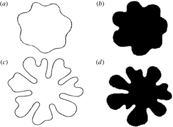
Figure 2 depicts the interface predicted from the numerical simulations of the present study with those obtained experimentally by Dias et al. (Reference Dias, Alvarez-Lacalle, Carvalho and Miranda2012). Results for two flow conditions with a mobility ratio
 $M=450$
, for
 $\unicode[STIX]{x1D70E}=8.9\times 10^{-3}$
and
 $\unicode[STIX]{x1D70E}=5.0\times 10^{-3}$
are shown with their corresponding experimental results at
 $(Ca_{m}=112,T_{f}=65)$
and
 $(Ca_{m}=200,T_{f}=40)$
, respectively. It is clear that the numerical simulations predict the same number of fingers as those observed in both experiments with almost identical overall structures. In particular the main morphological features of the interface including the tip-splitting instability in figure 2(a,c) have been well reproduced. This concordance between the predictions of the numerical simulations and the experimental measurements can be actually considered as excellent given the numerous uncertainties regarding the location of the injection and other sources of differences such as the uniformity of the cell gap as well as the plate surface in the experimental set-up.
Results at
 $M=450,\unicode[STIX]{x1D70E}=8.9\times 10^{-3}$
(
 $Ca_{m}=112$
,
 $T_{f}=65$
) (a,b), and at
 $M=450,\unicode[STIX]{x1D70E}=5.0\times 10^{-3}$
(
 $Ca_{m}=200$
,
 $T_{f}=40$
) (c,d) and at constant injection rate based on (a,c) simulation results, (b,d) experimental results from Dias et al. (Reference Dias, Alvarez-Lacalle, Carvalho and Miranda2012).

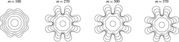
The numerical convergence was also examined for cyclic time-dependent injection flows by testing for different resolutions. Figure 3 shows a typical example for establishing the numerical convergence and shows the interfacial contours for
 $M=180$
,
 $\unicode[STIX]{x1D70E}=1.5\times 10^{-2}$
, and a period
 $T=2.80$
. Convergence appears to be achieved for the case where
 $m=300$
. The number and structure of the fingers are virtually unchanged for similar number of grid points. These conditions of flow, namely the mobility ratio and the surface tension, are within the range of the parameters considered in this study, and are evaluated later in § 4.
Numerical convergence results for a time-dependent displacement based on different grid sizes.
 $M=180,\unicode[STIX]{x1D70E}=1.5\times 10^{-2}$
and
 $T=2.80$
.

In the following section results for the effects of the variation of the injection flow period are analysed and a new resonance-like phenomenon is presented and characterized.
4 Results
A series of simulations were conducted to determine the effects of the period
 $T$
on the growth of instabilities. To do so, contours of the interface were tracked in time for different values of the period under fixed
 $M$
and
 $\unicode[STIX]{x1D70E}$
. In analysing the results, it was found that similar interfacial profiles were observed except for a specific value of the period that we shall refer to as the resonance period;
 $T_{res}$
. At such particular values of the period, fingers developed in a very distinctive manner not only in terms of their numbers but also in terms of their overall morphology. The interfacial growth was further analysed both at the observed period, where substantial deviations in morphology were noted, and at values very close to that period. To illustrate this new and unexpected phenomenon, contour plots of the interface are presented for different periods
 $T$
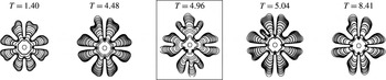
. Figure 4 shows the progression of the interfaces up to the point of breakthrough under five different periods of injection. The parameters that govern the flow are the mobility ratio
 $M=180$
and surface tension
 $\unicode[STIX]{x1D70E}=1.5\times 10^{-2}$
. Many other periods have also been evaluated, and for brevity only some samples of the results are shown. It was found that for all periods that have been examined except one, eight distinct fingers develop early in the flow and grow independently with virtually the same morphology. However for a particular period
 $T_{res}=4.96$
, the number of primary fingers that evolve distinctively from one another has decreased to just four fingers (see boxed finger structures in figure 4). This particular value of the period leads not only to different numbers of fingers but also to a morphology that is considerably distinct from that of all the other periods. In particular, for this value of the resonance period, strong tip splitting is observed on the dominant fingers that leads to two or three well developed sub-fingers at the fore front of the flow. As shall be seen later, other morphology changes such as the growth of secondary fingers and side branching can be observed at the resonance period. It should be noted that the differences in the structure of the interface at the special period can be actually also seen in the early stages of the flow.
Interfacial profiles up to the breakthrough for
 $M=180,\unicode[STIX]{x1D70E}=1.5\times 10^{-2}$
.

A further investigation of this phenomenon was carried out for other values of
 $M$
and
 $\unicode[STIX]{x1D70E}$
. Modifying these parameters affects the structure of viscous fingers, however, the phenomenon of resonance was found consistently in all examined cases. Again the interfacial instability was evaluated both at the period where substantial deviations in morphology occurred, and at values very close to those periods.
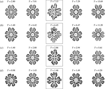
To show this effect, figure 5 displays samples of results for four different values of the mobility ratio
 $M=165,175,190$
and
 $200$
, and at a fixed
 $\unicode[STIX]{x1D70E}=1.5\times 10^{-2}$
. In each case, a particular value of the period leads to strong changes in the interfacial structure that can be traced to the early stages of the flow. For each resonance period identified by a box in figure 5, the number of fingers is different from all other periods and the structure of the interface has strongly changed with more complex fingers exhibiting multiple splitting, side branching as well as the growth of fingers at the base of some dominant fingers. These changes in the interface morphology also result in non-symmetric structures when compared to the other values of the injection flow period. Based on the results in figures 4 and 5, it can be concluded that there is a clear trend for the value of the resonance period
 $T_{res}$
to decrease with increasing
 $M$
.
Interfacial profiles up to the breakthrough for
 $\unicode[STIX]{x1D70E}=1.5\times 10^{-2}$
at: (a)
 $M=165$
, (b)
 $M=175$
, (c)
 $M=190$
and (d)
 $M=200$
.

Another important consideration is the effect of
 $\unicode[STIX]{x1D70E}$
under a fixed value of
 $M$
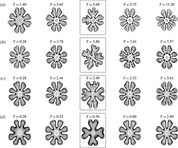
. Figure 6 depicts the evolution of the contour profiles up to the point of breakthrough at a fixed mobility ratio of
 $180$
and at four different values of the surface tension. Similar to what is observed in figures 4 and 5, a special value of the period
 $T_{res}$
can be easily identified. Such resonance period results in a lower number of primary fingers compared to that resulting from all other examined periods. Here too, the interface at the resonance period exhibits more intricate finger structures that result from different mechanisms such as complex tip splitting and side branching, which are not observed at the other values of the period. Moreover, from the values of the resonance period in figures 4 and 6,
 $T_{res}$
appears to decrease as
 $\unicode[STIX]{x1D70F}$
increases.
Interfacial profiles up to the breakthrough for
 $M=180$
at: (a)
 $\unicode[STIX]{x1D70E}=1.4\times 10^{-2}$
, (b)
 $\unicode[STIX]{x1D70E}=1.6\times 10^{-2}$
, (c)
 $\unicode[STIX]{x1D70E}=1.75\times 10^{-2}$
and (d)
 $\unicode[STIX]{x1D70E}=2.0\times 10^{-2}$
.

Overall, the contour plots indicate that the number of primary fingers is lower and that there is considerable change in the fingers structures at
 $T_{res}$
.
To characterize the previously reported trends, the number of fingers was determined and tracked in time for different values of
 $T$
,
 $M$
and
 $\unicode[STIX]{x1D70E}$
using a spectral analysis of the interface. To this end, the interface was cast as a series of data points in a
 $radius$
vs.
 $angle$
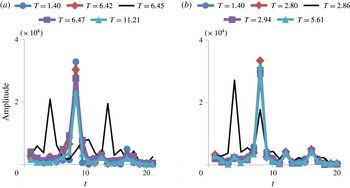
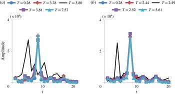
plot, and the Fourier transform of the data points was determined. Examples of typical Fourier spectra are depicted in figure 7 for
 $\unicode[STIX]{x1D70E}=1.5\times 10^{-2}$
,
 $M=175$
and
 $M=190$
, and at different values of the period
 $T$
, and figure 8 for
 $M=180$
, at
 $\unicode[STIX]{x1D70E}=1.6\times 10^{-2}$
and
 $\unicode[STIX]{x1D70E}=1.75\times 10^{-2}$
. It can be seen that for all examined periods except at
 $T_{res}$
for each set of conditions, the same clear and distinctive peak is obtained, which corresponds to the dominant mode, or the number of fingers that are observed at the interface. The spectra become however very different at the resonance period (black line), where the same mode does not dominate, but there appears to be other modes that play a significant role in the shape of the interface. This reflects the complex finger structures resulting from tip splitting, side branching and other instability mechanisms that were identified more clearly at the resonance period.
Fourier transform spectra of interfaces at breakthrough for
 $\unicode[STIX]{x1D70E}=1.5\times 10^{-2}$
at: (a)
 $M=175$
and (b)
 $M=190$
.

Fourier transform spectra of interfaces at breakthrough for
 $M=180$
at: (a)
 $\unicode[STIX]{x1D70E}=1.6\times 10^{-2}$
and (b)
 $\unicode[STIX]{x1D70E}=1.75\times 10^{-2}$
.

In order to further describe this phenomenon of resonance, the minimum and the maximum radii of the interface were tracked with time. The minimum radius is found by determining the point in the interface that is the closest to the centre of the domain, whereas the maximum radius is determined by identifying the farthest point from the interface to the centre. The concepts of
 $R_{min}$
and
 $R_{max}$
are somewhat analogous to what Huang & Chen (Reference Huang and Chen2015) reported by measuring the position of the inward fingers and the outward fingers, respectively. Comparatively, a small value of
 $R_{min}$
and/or a large value of
 $R_{max}$
would be indicative of a more unstable interface, whereas a large value of
 $R_{min}$
and/or a small value of
 $R_{max}$
would be a characteristic feature of a less unstable interface. For a stable circular interface,
 $R_{min}=R_{max}$
, whereas for an unstable interface
 $R_{min}<R_{max}$
. It should however be noted that these radii can be considered only as one of many other quantitative measures to be used to characterize the instability, since interfaces with different morphologies and numbers of fingers can still result in the same maximum or minimum radius.
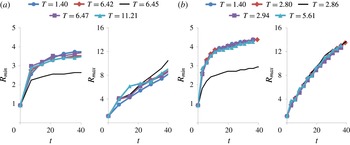
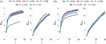
Variations of the maximum and minimum radii with time for different values of the period including the resonance one are depicted in figure 9 for a fixed surface tension and two values of the mobility ratio;
 $M=175$
and
 $M=190$
. Similar trends are shown in figure 10 for fixed mobility ratio
 $M=180$
and two values of the surface tension;
 $\unicode[STIX]{x1D70E}=1.6\times 10^{-2}$
and
 $\unicode[STIX]{x1D70E}=1.75\times 10^{-2}$
. It can be seen that for all periods,
 $R_{min}$
increases with time and tends to plateau at later times, while
 $R_{max}$
increases monotonically with time and does not level off even at later times. More interestingly, it is found that both radii do not vary monotonically with the period of the injection flow, and in particular
 $R_{min}$
at the resonance period is substantially smaller than for all other periods
 $T$
under the same conditions of
 $M$
and
 $\unicode[STIX]{x1D70E}$
. This trend, although shown here only for some representative values of the mobility ratio and the surface tension, has been observed systematically for all other cases. This represents another quantitative measure to identify the resonance period. The results from the variations of the maximum radius with the period are not however as conclusive, with
 $R_{max}$
at the resonance period, being sometimes larger and sometimes smaller than those at other periods, with variations not being as clearly observable as for
 $R_{min}$
. This result in the case of the maximum radius is not surprising since this region where the finger tips extend far from the centre, is mainly occupied by the displaced fluid as opposed to the minimum radius one where the displacing fluid is predominant.
 $R_{min}$
and
 $R_{max}$
with time for
 $\unicode[STIX]{x1D70E}=1.5\times 10^{-2}$
at: (a)
 $M=175$
and (b)
 $M=190$
.

 $R_{min}$
and
 $R_{max}$
with time for
 $M=180$
at: (a)
 $\unicode[STIX]{x1D70E}=1.6\times 10^{-2}$
and (b)
 $\unicode[STIX]{x1D70E}=1.75\times 10^{-2}$
.

The previous results show that at the resonance period, the interface can be characterized by an increased instability, which appears to emerge earlier and be stronger than for the other flow periods. This is well illustrated by the plots depicting the variations of the minimum radius with time, where for
 $T_{res}$
, the growth of the minimum radius is consistently attenuated, thus allowing the growth of stronger fingers. One of the other features of resonance is the change in the number of dominant fingers that was shown through the Fourier spectra at breakthrough. For
 $T_{res}$
, fingers grow large and tend to become nonlinear, exhibiting considerable finger splitting and spreading. What is also worth noting, is that the deviation in the number of fingers and their morphology at the resonance period actually starts to develop in the early stages of the flow displacement, as can be seen from the interface contours in the early times of the flow. This indicates that some insight into the mechanisms of this resonance-like phenomenon can be traced back to the first stages of the flow development.
In order to gain some insight into the flow dynamics and the mechanisms behind the reported resonance phenomenon, let us examine some results from linear stability analysis of displacements in a radial geometry. Based on the study by Miranda & Widom (Reference Miranda and Widom1998), the following expression of the dimensionless growth rate corresponding to the fastest growing mode can be obtained:
 $$\begin{eqnarray}\unicode[STIX]{x1D706}(n_{max})=\left[\frac{Q}{2R^{2}}\left(\frac{M-1}{M+1}n_{max}-1\right)-\frac{\unicode[STIX]{x1D70E}M}{(M+1)R^{3}}n_{max}(n_{max}^{2}-1)\right],\end{eqnarray}$$
where
 $n_{max}$
is the fastest growing mode, which itself varies with time and that is determined as the closest integer to the square root of
 $\unicode[STIX]{x1D6E4}$
(Miranda & Widom Reference Miranda and Widom1998);
 $$\begin{eqnarray}\unicode[STIX]{x1D6E4}=\frac{1}{3}\left[\frac{Q\cdot R(M-1)}{2M\unicode[STIX]{x1D70E}}+1\right].\end{eqnarray}$$
In the present study involving a sinusoidal injection, the flow rate
 $Q(t;T)$
and the radius
 $R(t;T)$
are related as:
 $$\begin{eqnarray}R^{2}(t;T)=1+\int _{0}^{t}Q(\unicode[STIX]{x1D701};T)\,\text{d}\unicode[STIX]{x1D701}.\end{eqnarray}$$
One must bear in mind that the above expressions are based on linear stability analysis and hence may not be valid in the full nonlinear regime and furthermore, the growth rates including the one corresponding to the most dangerous modes are themselves time dependent and cannot be simply associated with the number of fingers that develop at the interface. Still, and even though it is not possible to determine an explicit expression for the growth rate associated with the most dangerous mode, equation (4.1) indicates that there would be a nonlinear relationship between the injection flow period, the two parameters
 $\unicode[STIX]{x1D70E}$
and
 $M$
and time
 $t$
, that leads to the strongest instability:
 $$\begin{eqnarray}\mathfrak{F}[M,\unicode[STIX]{x1D70E},t;T]=0.\end{eqnarray}$$
The results of the present study indicate that except for a special period;
 $T_{res}$
, the dominant modes are not affected by variation in the flow injection period. These modes however change significantly at the resonance period that is expected to correlate with some flow characteristic time
 $t_{ch}$
related to the forces behind the flow instability.
The instability in this problem is determined by a competition between the viscous forces and surface tension. In order to characterize these forces, we will adopt the original notations based on dimensional quantities. A length scale that characterizes the instability can be determined from the ratio of the surface tension and the viscous (pressure drop) forces, as:
 $$\begin{eqnarray}L_{ch}\equiv \frac{\unicode[STIX]{x1D70E}}{\unicode[STIX]{x0394}P}\propto \frac{\unicode[STIX]{x1D70E}K}{(\unicode[STIX]{x1D707}_{2}-\unicode[STIX]{x1D707}_{1})\unicode[STIX]{x1D719}_{0}R_{0}^{2}}.\end{eqnarray}$$
The corresponding characteristic time is:
 $$\begin{eqnarray}t_{ch}\equiv \frac{L_{ch}}{U_{0}}\propto \frac{1}{(\unicode[STIX]{x1D707}_{2}-\unicode[STIX]{x1D707}_{1})}\frac{\unicode[STIX]{x1D70E}K}{\unicode[STIX]{x1D719}_{0}^{2}R_{0}^{3}},\end{eqnarray}$$
Which in dimensionless form reads:
 $$\begin{eqnarray}t_{ch}^{\ast }=\frac{M\unicode[STIX]{x1D70E}^{\ast }}{(M-1)}.\end{eqnarray}$$
We will now proceed to analysing the relationship between the flow characteristic time and the flow injection period. To do so, we will revert to dimensionless notation and drop the star.
First, it should be noted that for the range of values of the mobility ratio
 $M$
that were examined in this study
 $M\sim O(100)$
, the characteristic time
 $t_{ch}$
is equivalent to the dimensionless surface tension based on the properties of fluid2;
 $\unicode[STIX]{x1D70E}$
. Moreover, the dimensionless characteristic time represents a ratio of the surface tension to viscous forces, and for the range of dimensionless surface tension reported in this study;
 $\unicode[STIX]{x1D70E}\sim O(10^{-2})$
, it can be assumed that the flow instability is dominated by viscous forces. It is also expected that the resonance phenomenon is a result of an association between the ‘natural’ characteristic frequency of the flow;
 $\unicode[STIX]{x1D714}_{ch}\propto 1/t_{ch}$
and the frequency of the injection flow;
 $\unicode[STIX]{x1D714}_{f}=2\unicode[STIX]{x03C0}/T$
. Therefore the resonance period will be mainly a function of the flow characteristic time and the fluids mobility ratio;
 $$\begin{eqnarray}T_{res}=\mathfrak{G}[M,t_{ch}(M,\unicode[STIX]{x1D70E})].\end{eqnarray}$$
As noted earlier, the above functional dependence is expected to be nonlinear.
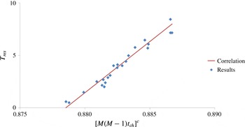
Figure 11 depicts the variation of the resonance period with
 $[M(M-1)t_{ch}]=(\unicode[STIX]{x1D70E}\unicode[STIX]{x1D6FD}_{1}/\unicode[STIX]{x1D719}_{0}R_{0}^{3})(\unicode[STIX]{x1D6FD}_{1}/\unicode[STIX]{x1D6FD}_{2})$
for a wide range of parameters. It is clear that all of the data can be characterized by a decay where:
 $$\begin{eqnarray}T_{res}\propto [M(M-1)t_{ch}]^{-0.02}.\end{eqnarray}$$
This correlation was actually tested and helped in the determination of the resonance period for other values of
 $M$
and
 $\unicode[STIX]{x1D70E}$
with very good accuracy.
Variation of
 $T_{res}$
with
 $M(M-1)t_{ch}$
. Points are data from simulations and the solid line corresponds to the correlation.

5 Conclusions
In this study, the dynamic behaviour of the interface of two immiscible fluids undergoing time-dependent injection in a homogeneous porous medium was analysed. The injection flow consisted of a cyclic sinusoidal function of period
 $T$
and unit amplitude. Such a flow is governed by three major parameters, namely the dimensionless period
 $T$
, surface tension
 $\unicode[STIX]{x1D70E}$
and mobility or equivalently viscosity ratio
 $M$
. It was found that at a critical value of the period of the injection flow, the interface between the fluids deviates significantly from the trend observed for all other examined periods under the same conditions of
 $\unicode[STIX]{x1D70E}$
and
 $M$
. These deviations, which can be observed even in the early stages of the displacement, are manifest in terms of different numbers of fingers as well as in the form of very distinctively different structures of the instabilities at the interface. This critical value of the period is suspected to be associated with a resonance-like dynamics between the external forcing by the injection flow and the response of the fluids based on their characteristic viscosities and surface tension. The phenomenon was characterized through a spectral analysis of the interface that shows a clear deviation in the Fourier spectrum at the resonance period;
 $T_{res}$
. A quantitative analysis based on the time variations of the minimum and maximum radii also allowed to clearly identify the deviation in the flow dynamics at
 $T_{res}$
where a smaller minimum radius
 $R_{min}$
was systematically observed at the resonance period. Even though a deviation was also reported in the case of the maximum radius, it was not as prominent for
 $R_{min}$
. The reported phenomenon was analysed using results based on linear stability analysis of radial immiscible displacements and an interpretation of the observed changes based on a resonance-like dynamics between the external forcing by the injection flow and the response of the fluids based on their characteristic viscosities and surface tension. Under conditions represents by the range of parameters examined in this study and that correspond to viscously dominated displacements, a model for the variation of the resonance period
 $T_{res}$
in terms of a flow characteristic time and the fluids mobility ratio
 $M$
is presented. The reported phenomenon and the proposed model offer the possibility of using this hydrodynamic interfacial instability and the resonance induced by the oscillatory injection flow as a possible means to determine physical properties, namely the fluids viscosities and surface tension.
Acknowledgements
The authors acknowledge financial support from the Natural Sciences and Engineering Research Council of Canada (NSERC) and the use of the computing resources of WestGrid. The authors also thank anonymous referees for valuable comments.