I. INTRODUCTION
According to the Commission on Macromolecular Nomenclature of the IUPAC Macromolecular Division, the heterogeneous copolymers are ideally synthesized in a chain-propagation process exhibiting first-order Markovian statistics with two different reactivity ratios (r 1 and r 2) between monomers and comonomers and with a significant drift in feed compositions (F).Reference Ring, Mita, Jenkins and Bikales1 Such a process corresponds to the free-radical copolymerization with a single-site catalyst in the batch reaction. Normally, monomers are treated as the crystallizable regular sequences and comonomers are regarded as the noncrystallizable irregular sequences.Reference Hu, Mathot and Frenkel2 When the propagation probabilities are not constant either within one chain or from one chain to the next, the copolymer sample will be a mixture of chains with quite different comonomer contents and sequence distributions.Reference Hu, Mathot and Frenkel2 In reality, heterogeneous copolymers are even synthesized via multisite catalysts besides single-site catalysts. An example is linear low-density polyethylene (LLDPE) produced with heterogeneous-type Ziegler–Natta catalysts.Reference Mathot3–Reference Karbashewski, Kale, Rudin, Tchir, Cook and Pronovost6 Even so, the heterogeneous sequences of copolymers determined by the single-site catalyst can be a good representative for heterogeneous copolymers in our study.
Conventionally, the heterogeneous copolymers with an extreme diversity in comonomer contents can be regarded as a binary mixture with one fraction rich and another fraction poor in comonomer contents. On cooling from a high temperature, their molecular segregation before crystallization has actually been regarded as liquid–liquid demixing in the blend.Reference Mirabella and Ford7–Reference Chen, Shanks and Amarasinghe12 The phase separation phenomenon in such kinds of polymer blends have received much experimental study in recent years.Reference Wang, Shimizu, Kim, Hobbie, Wang and Han13–Reference Katsumi, Wang, Wang, Matsuba, Kim and Han16 In dynamic Monte Carlo (MC) simulations of heterogeneous copolymers, we have observed liquid–liquid demixing prior to crystallization on cooling.Reference Hu, Mathot and Frenkel2, Reference Hu and Mathot17, Reference Ma, Zha, Hu and Han18 Such a demixing is driven purely by the component-selective crystallizability.Reference Hu and Mathot17, Reference Ma, Zha, Hu and Han18 Crystallization occurs mainly in the phase poor in comonomer sequences. For normal heterogeneous copolymers, especially when comonomer distributions are not so extremely heterogeneous, how the copolymer fractions with intermediate comonomer contents between the above two extremities affect the crystallization behavior of heterogeneous copolymers is worthy of further study. An example of such practical cases is the high impact propylene-co-ethylene polymers containing quite significant fractions with intermediate comonomer contents.Reference Cai, Luo, Ma, Wang and Tan19–Reference Zhang, Chen, Shangguan and Zheng23 Experimental observations have revealed special crystal morphologies in neat association with their mechanical performances.Reference Fu, Fan, Zhang and Feng21–Reference Zhang, Chen, Shangguan and Zheng23
In this article, we perform dynamic MC simulations to compare crystallization behaviors between two series of heterogeneous copolymers separated with strong and weak heterogeneities of comonomer distributions. The results will demonstrate the importance of the copolymer fractions with intermediate comonomer contents in the phase transition behaviors of heterogeneous copolymers.
In the following sections, we first introduce the preparation of two series of heterogeneous copolymer samples, and then we give a simple description about the models and the simulation algorithm used here. After that, we report the simulation results. The article ends with a summary of our conclusions.
II. SAMPLE PREPARATION AND SIMULATION TECHNIQUES
A. Sample preparation
We put 1920 chains, each occupying 128 consecutive sites, in a cubic lattice box with a linear size of 64, so the occupancy density of the sample is 0.9375 to mimic the bulk polymer phase. We set up the heterogeneous sequences in copolymers with various average comonomer mole fractions (0.06, 0.12, 0.24, 0.36, 0.44, and 0.54, respectively, meaningful only for comparisons in modeling but not in reality) and with two kinds of sequence distributions (like in the batch reactions separated with two different single-site catalysts). We assumed that the sequences of monomers and comonomers in all the chains align consecutively on a long single macromolecule with its length as large as covering over all the monomers and comonomers in the sample. Along this single macromolecule, the first sequence unit is labeled as being a monomer (denoted as 1) or a comonomer (denoted as 2) according to the probability determined by the initial feed composition, and the next unit and so on are labeled according to the specific propagation probabilities determined by the preset reactivity ratios and the drifting feed compositions in batch reactions. For two series of heterogeneous copolymers, we separately set sample series A with r 1 = 24.7 and r 2 = 0.017, as well as sample series B with r 1 = 14.99 and r 2 = 0.495. The initial feed compositions were selected to meet the preset average comonomer contents.
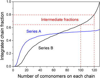
Figure 1 shows the integrated distribution curves of copolymers for their specific comonomer contents, in two heterogeneous copolymer samples separately belonging to two sample series, but both with an average comonomer content of 0.54, as for example. In series A, because r 1 is far from r 2, monomers have a much higher priority in reaction. Therefore, upon the batch reaction, monomers will be depleted at the early stage and the copolymer fractions containing high comonomer content will be yielded at the later stage. Such copolymers can be divided into two fractions: one fraction appears rich of monomer sequences and thus crystallizable and another fraction appears rich of comonomer sequences and thus noncrystallizable (their boundaries were assumed to locate at 127 comonomer units). In contrast, in series B, monomers will be depleted slowly upon the batch reaction and a significant copolymer fraction with intermediate comonomer content between two extremities will be yielded. Such copolymers can be divided into three fractions: two extremes are similar with series A, and the third fraction contains intermediate comonomer contents (Their boundaries were assumed at 100 and 120 comonomer units, separately. These boundaries were just tentative and arbitrary selections for the representative of intermediate fractions between two extremities, which are mainly noncrystalline but contain certain amounts of monomer sequences.)
Integrated distributions of copolymers on the numbers of comonomer units on each chain, for two samples both containing the average comonomer content 0.54. The red box with dashed lines denotes the fractions of intermediate comonomer contents from 100 to 120 comonomers between two extremities in sample series B.

B. Microrelaxation model and Metropolis algorithm
In our simulations, the model and the sampling method were the same as reported in Ref. Reference Hu, Mathot and Frenkel2. We used periodic boundary conditions in the cubic lattice box. The microrelaxation model allowed each (co)monomer to jump into its vacant neighbor, with partial sliding diffusion along the chain if necessary, presumably similar with the local bending and sliding on the chain molecules.Reference Hu, Mathot and Frenkel2 The bonds on the chain can be oriented either along 6 lattice axes or along 12 face diagonals and 8 body diagonals, so the coordination number of a (co)monomer can be as high as 6 + 12 + 8 = 26. Upon microrelaxation, (co)monomers would not occupy doubly on each lattice site, and the bonds could not cross over each other, to mimic the volume exclusion of polymers. To mimic the ethylene copolymers grafted with large side groups, we further set up a rule to prevent the large comonomer units diffusing into crystalline regions of the small monomer units. We actually did as follows: if a comonomer was going to slide into a bond position previously occupied by two monomers, we examined whether that monomer bond contained more than one parallel neighbor of monomer bonds. Since the parallel-packed monomer bonds were considered as locally crystalline, this trial move would be rejected. We used this case as general for ethylene-based copolymers, but it should be noted that the sliding effect itself affects more crystallization rather than demixing,Reference Hu, Karssenberg and Mathot24 and propylene–ethylene copolymers still allow a significant amount of propylene units to be mixed with crystalline ethylene units.Reference De Rosa, Auriemma, de Ballesteros, Resconi and Camurati25
In each step of microrelaxation, we used the conventional Metropolis sampling algorithm with the potential energy

that was contributed purely by the parallel-packed monomer bonds. Only the monomer sequences are crystallizable and hence contain the packing energy E p. So, we got a change of potential energy pE p, where p is the net result in the change of the total number of such parallel monomer bonds. In principle, potential energy penalties for the gauche-trans conformation changes on the chain as well as for the mixing pairs between monomers and comonomers could also have been included. For the sake of simplicity, we supposed that the chains were fully flexible and that the mixing between monomers and comonomers was athermal. The packing energy difference between monomer sequences and comonomer sequences has made a strong enough mixing interaction between two extreme fractions, which drives a spontaneous liquid–liquid demixing upon cooling from high temperatures.Reference Hu, Mathot and Frenkel2, Reference Hu and Mathot17 Since there are volume-exclusion interactions between polymers, crystal growth on cooling will spread over the sample system without overlapping and generate certain crystallinity depending on the comonomer content. An extreme case is the crystallizable homopolymer, which reaches almost full crystallinity on cooling, as reported previously for a comparison to the copolymer cases.Reference Hu, Mathot and Frenkel2
C. Temperature-scanning programs
The homogeneous phases of bulk copolymers were prepared by performing enough number of microrelaxation moves under athermal conditions. We then stepwise changed the reduced temperature kT/E p from 6 to 2, in step length 0.01 and step period 300 MC cycles, where k is the Boltzmann’s constant and one MC cycle is defined as the total amount of trial moves with one trial move per (co)monomer averaged over the sample system. Such a scanning program is similar like in a differential scanning calorimetry measurement. During each step, the first 100 MC cycles were discarded for equilibration. Data were collected as an average over the subsequent 200 MC cycles. In this cooling temperature range, crystallization and liquid–liquid demixing were expected to occur spontaneously. After the cooling steps, the crystallized samples were heated back with the same scanning rates from 2 to 6, where melting and liquid–liquid mixing were expected to occur spontaneously.
To monitor crystallization/melting during the temperature-scanning processes, the crystallinity was traced, which was defined as the fraction of monomer bonds containing more than five neighboring parallel monomer bonds. In the crystalline region, the maximum crystallizable monomer bonds packing in parallel around one monomer bond can be 24, which is the coordination number of 26 minus 2 consecutive bonds connected along the chain. While in the amorphous region, the amount of parallel packing is usually close to zero. To distinguish the amorphous region from the partially crystalline region, we used a criterion of five parallel bonds that would effectively identify the bond status from the amorphous state to the crystalline state, even for those bonds located at the crystallite surface with rich defects. Meanwhile, to monitor the liquid–liquid demixing process, the mixing parameter was traced as well, which was defined as the mean fraction of neighboring sites of each monomer occupied by other comonomers. This quantity is sensitive to the change in the local environment of each monomer due to phase separation in copolymers with various compositions.
III. SIMULATION RESULTS
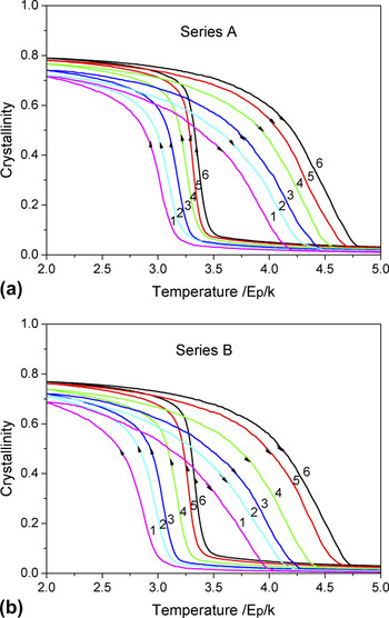
For two series of heterogeneous copolymer samples with various average comonomer contents, we collected their crystallinity curves in both cooling and heating processes, as summarized in Fig. 2. As usual, higher comonomer contents lead to lower crystallization and melting temperatures. But in a comparison between Fig. 2(a) for series A and Fig. 2(b) for series B, one can see that the samples in series B exhibit even lower crystallization and melting temperatures than those in series A. Such a shifting to lower temperatures must be related with the significant fractions of intermediate comonomer contents between two extremities in the sample series B.
Crystallinity curves on cooling and then heating (see arrows on the curves) for (a) samples in series A and (b) samples in series B, with various average comonomer mole fractions as denoted nearby (1—0.06, 2—0.12, 3—0.24, 4—0.36, 5—0.44, and 6—0.54).

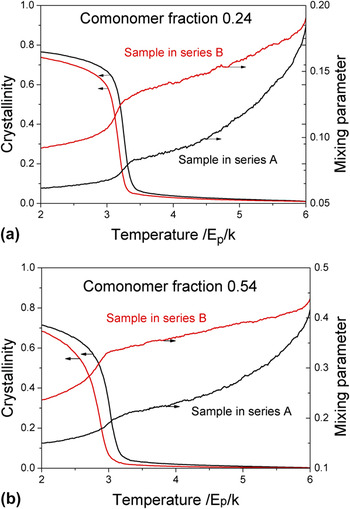
We further compared their mixing parameter curves on cooling for two samples both with the same average comonomer mole fractions, but belonging to two series. The results are shown on Figs. 3(a) and 3(b), separately for 0.24 and 0.54 mol fractions (similar results in all the series). One can see that, in company with the shifting to lower crystallization temperatures, the sample in series B exhibits a depressed liquid–liquid demixing prior to crystallization on cooling. This behavior implies that the subsequent crystallization occurs in a relatively mixed system, and hence in a lower temperature region. This is because the melting point, in principle, decreases with the dilution due to the large mixing entropy of short monomer and comonomer sequences.
Crystallinity and mixing parameter curves on cooling for the sample of series A (black curves) and the sample of series B (red curves) as denoted nearby, with average comonomer mole fractions of (a) 0.24 and (b) 0.54, respectively. The arrows are indicating the corresponding axes.

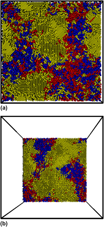
The comparison of the cooling curves between sample A and sample B in Fig. 3 reveals that, the copolymer fractions with intermediate comonomer contents could significantly depress the liquid–liquid demixing before crystallization on cooling, leading to different mixing concentrations for subsequent crystallization. As shown in Fig. 3(b), right before crystallization, the mixing parameters before crystallization have been shifted up from 0.2 to 0.35. The larger mixing parameter corresponds to a lower concentration of monomers for crystallization. Would the intermediate fraction behave like a compatibilizer to enhance the miscibility of two extreme fractions? To convince this judgment, we observed the crystal morphology obtained at low temperatures upon the cooling process. Figure 4 shows the snapshots of the sample in series B with the average comonomer mole fraction of 0.54 at a reduced temperature of 2. Three copolymer fractions are shown in yellow, red, and blue, separately. The yellow fractions can crystallize but within small domains. These small domains are surrounded with the red intermediate fractions, implying that the intermediate fractions behave like a surfactant to stabilize the interfaces between blue and yellow fractions.
Snapshots of the sample in series B with the average comonomer mole fraction of 0.54 at the reduced temperature of 2. (a) The front surface in a cubic lattice with periodic boundary conditions; (b) the two-third depth section surface. The polymer bonds are drawn in cylinders. The copolymer fractions containing most of monomer sequences are shown in yellow, the intermediate fractions are shown in red, and the fractions containing most of comonomer sequences are shown in blue.

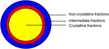
The role of the intermediate fractions becomes clear now. They enhance the mixing between crystallizable fractions and noncrystallizable fractions and locate mainly near the interfaces between these two extreme fractions. So they can be regarded as a compatibilizer or a surfactant in the incompatible polymer blend. Therefore, we can construct an illustration to explain the roles of three fractions in the samples of series B. Figure 5 shows the illustration. The crystallizable fractions form the crystalline hard domains, the intermediate fractions cover their surfaces, and the noncrystallizable fractions form a continuous matrix. The similar model has been proposed for experimental observations on the high impact polypropylene copolymers.Reference Chen, Shangguan, Zhang, Chen, Harkin-Jone and Zheng22, Reference Zhang, Chen, Shangguan and Zheng23
Illustration of the phase structure for three fractions in the samples of series B, obtained at low temperatures. The yellow area is the crystallizable fraction domain, the blue area is the noncrystallizable fraction matrix, and the red area is the intermediate fraction to cover the interfaces.

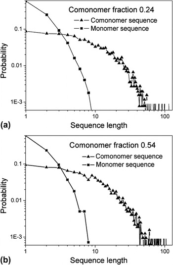
The compatibilizers or the surfactants are conventionally featured with amphiphilicity at two ends of molecules. Would the intermediate fractions appear as a diblock copolymer? We made statistics on the probability of comonomers occurring at each sequence unit along the chain for 0.0594 and 0.1526 intermediate fractions separately for the sample series B with the average comonomer mole fractions of 0.24 and 0.54. We found that comonomers are almost homogeneously distributed on each chain. The statistics was made along the sequences of each chain same as those copolymerization sequences. So such a homogeneous distribution is a natural result of copolymerization. We also made the probabilities of monomer and comonomer sequence lengths, as shown in Figs. 6(a) and 6(b). One can see that the sequence lengths are rather short although comonomer sequences are longer than monomer sequences. In addition, the sequence distributions in the same intermediate fractions are rather independent of the average comonomer contents. Therefore, the amphiphilicity on the copolymer fractions with intermediate comonomer contents occurs at the short monomer and comonomer sequences on each copolymer chain.
Distributions of monomer and comonomer sequence lengths along 128-mer copolymer chain with the intermediate comonomer content. The results are based on the statistics over about 400 copolymers in the sample of series B with the average comonomer mole fraction of (a) 0.24 and (b) 0.54.

IV. CONCLUSIONS
We performed dynamic MC simulations of heterogeneous copolymers to address the role of copolymer fractions with intermediate comonomer contents in the crystallization process on cooling. The results show that the intermediate fractions depress the prior liquid–liquid demixing on cooling, stabilize the interfaces between the other two extreme fractions, and thus weaken the subsequent crystallization behavior on cooling. The simulations reproduced some experimental observations on heterogeneous copolymers. In conclusion, the intermediate fractions can be regarded as a compatibilizer or a surfactant, although the sequence distributions are rather short and quite homogeneous on copolymers, far from like a diblock copolymer.
ACKNOWLEDGMENTS
We are grateful to the stimulating discussions offered by Prof. Yonggang Shangguan at Zhejiang University. The financial support from National Natural Science Foundation of China (Grant No. 20825415) and from the National Basic Research Program of China (Grant No. 2011CB606100) is appreciated.