
I. INTRODUCTION
It is well known that the hot deformation processes (forging, rolling, and extruding et al.) of metals and alloys are extremely complex and regarded as a crucial part in the industrial production. Reference Lentz, Gall, Schmack, Mayer and Reimers1–Reference Sun, Guo, Fu and Liu3 In this context, a considerable amount of research has been devoted to acquire the accurate predictability of the material models to simulate the deformation process. Moreover, the modeling of hot deformation behavior is generally established through the constitutive equations. Accordingly, a number of constitutive models have occurred through hot compressive or tensile experiments to clarify the relationship between the flow stress and deformation parameters (i.e., temperatures and strain rates) for different metals and alloys so as to better guide the hot working process. Reference Mehtedi, Musharavati and Spigarelli4–Reference Wang, Chandrashekhara, Rummel, Lekakh, Van Aken and O’Malley7
According to recent research, Samantaray et al. Reference Samantaray, Mandal and Bhaduri8 carried out a study to compare the predictability of Johnson–Cook (JC), modified Zerilli–Armstrong (ZA) and strain-compensated Arrhenius-type constitutive models for the flow behavior of 9Cr–1Mo steel, and eventually found that Arrhenius-type constitutive models revealed a higher prediction accuracy than the other models in the hot working domain. Abbasi-Bani et al. Reference Abbasi-Bani, Zarei-Hanzaki, Pishbin and Haghdadi9 introduced two phenomenological constitutive equations (Johnson Cook and Arrhenius-type ones) to depict the high temperature flow behavior of Mg–6Al–1Zn alloy during hot compression tests, and also concluded that the Arrhenius-type equations were more reliable for the material deformation process. Same as above, the investigations of the flow behavior of Al–0.62Mg–0.73Si aluminum alloy Reference Sun, Ye and Hu10 and ferritic stainless steel Reference Zhao, Jiang, Zu, Du, Zhang and Jiang11 still proved the prediction capability of the Arrhenius-type model was stronger than the Johnson–Cook model. Furthermore, a modified Arrhenius-type constitutive equation considering the effect of strain on material constant was developed under hot deformation conditions to describe the flow stress of different materials, such as Ti–20Zr–6.5Al–4V alloy, Reference Tan, Duan, Yang, Liu, Zhang and Liu12 aluminum alloy (AA2030 alloy, Reference Ashtiani and Shahsavari13 Al–Zn–Mg–Cu alloy, Reference Zhou, Lin, Deng and Jiang14 and AA6N01 alloy Reference Zhang, Ding, Dong, Zhao, Gao and Wang15 ), magnesium alloy (AZ81 alloy, Reference Changizian, Zarei-Hanzaki and Roostaei16 AZ31B alloy, Reference Yu17 and Mg–4Li–1Al alloy Reference Askariani and Hasan Pishbin18 ), 17%Cr ferritic stainless steel, Reference Gao, Liu, Misra, Liu and Yu19 AISI 420 stainless steel, Reference Cao, Di, Misra, Yi, Zhang and Ma20 Fe–21Mn–2.5Si–1.5Al steel, Reference Marandi, Zarei-Hanzaki, Haghdadi and Eskandari21 Nb–Ti micro alloyed steel, Reference Wu, Zhou, Cao, Liu and Wang22 and Nickel-based corrosion-resistant alloy (N08028). Reference Wang, Liu, Cheng, Zuo and Chen23 Additionally, based on modified Zerilli–Armstrong model, a thermo-viscoplastic constitutive model was proposed by Samantaray et al. Reference Samantaray, Patel, Borah, Albert and Bhaduri24 and used to successfully describe the flow behavior of IFAC-1 austenitic stainless steel under the hot working conditions. Nevertheless, a comparison between the modified Zerilli–Armstrong and the Arrhenius-type model about the flow behavior predictability of BFe10-1-2 cupronickel alloy also illustrated that the latter had a better performance. Reference Cai, Lei, Wang, Zhang, Miao and Li25 Similarly, Guan et al. Reference Guan, Ren, Zhao, Ma and Wang26 compared the predictability of a phenomenological constitutive equation and an empirical constitutive equation to model the flow behavior of Al–Zn–Mg–Zr alloy, and then found the latter had higher accuracy over wide range of strain rates and strains. By taking the temperature softening coefficient and strain rate sensitivity into account, an amended Fields–Backofen (FB) equation was applied to precisely describe the constitutive behavior of magnesium alloy (as-cast AZ31Bb alloy Reference Jia, Xu, Le, Fu, Ma and Tang27 and extruded AZ61 alloy Reference Tsao, Huang and Fan28 ) under hot compression tests. Meanwhile, the artificial neural network (ANN) model with a feed-forward back propagation has been evaluated during hot deformation process to predict the flow behavior of different materials, such as as-cast TC21 titanium alloy, Reference Zhu, Zeng, Sun, Feng and Zhou29 Ti600 alloy, Reference Han, Zeng, Zhao, Qi and Sun30 ZK60 alloy, Reference Qin, Pan, He, Li, Liu and Fan31 AZ81 magnesium alloy, Reference Sabokpa, Zarei-Hanzaki, Abedi and Haghdadi32 7050 aluminum alloy, Reference Quan, Wang, Li, Zhan and Xia33 20MnNiMo low carbon alloy, Reference Wang, Wang and Wang34 and Cu–0.4Mg alloy. Reference Ji, Yang, Li and Li35
On the other hand, researchers investigated the effect of rationalized processing parameters on microstructure evolution or mechanical properties of different metals and alloys, such as as-cast Ti60 titanium alloy, Reference Peng, Zeng, Wang, Zhao and Yu36 bainitic pipeline steel, Reference Soliman and Palkowski2 TRIP780 steel, Reference Sun, Guo, Fu and Liu3 316 L(N) austenitic stainless steel, Reference Samantaray, Mandal, Phaniraj and Bhaduri37 titanium alloy, Reference Guo, Fan, Yu and Yang38 aluminum alloy (AA2030 alloy, Reference Ashtiani and Shahsavari13 7050-H112 alloy, Reference Wang, Wang, Zhou, Dong and Jia39 and 7050 alloy Reference Wu, Li and Ma40 ) and dual super–alloy. Reference Liu, Yao, Ning, Nan, Guo, Qin and Shi41 It is worth noting that some typical metallurgical phenomena [dynamic recovery, dynamic recrystallization (DRX), work hardening behavior, grain boundary characteristic distribution] appeared at microstructure evolution during the hot deformation process and DRX can occur especially in face-centered cubic structure alloys with low stacking fault energy. Reference Gao, Liu, Misra, Liu and Yu19 Feng et al. Reference Feng, Zhang, Liu and Deng42 investigated the flow stress of Al–7.68Zn–2.12Mg–1.98Cu–0.12Zr alloy based on the kinetics of DRX and dislocation density theory and then analyzed the microstructure by combining Z–H parameter as well as processing map. Bobbili et al. Reference Bobbili and Madhu43 not only established the DRX kinetic equation of biomedical Ti–13Nb–13Zr alloy under the high temperature compression tests but also found the decrease of strain rate and increase of deformation temperature both promoted the process of DRX. Also, some investigators researched the DRX behavior of different metals and alloys, such as nickel-based super-alloy, Reference Chen, Lin, Wen, Zhang and He44 6X82 aluminum alloy, Reference Kai, Chen, Sun, Wang and Zhao45 stainless steel (ultra-pure 17%Cr ferritic, Reference Gao, Liu, Misra, Liu and Yu19 AISI 420, Reference Cao, Di, Misra, Yi, Zhang and Ma20 304 H austenitic, Reference Mirzadeh, Cabrera, Najafizadeh and Calvillo46 and LDX 2101 duplex Reference Haghdadi, Martin and Hodgson47 ), AZ31 and ME21 magnesium alloys, Reference Gall, Huppmann, Mayer, Müller and Reimers48 and nickel–chromium alloy (800H). Reference Cao, Di, Zhang, Zhang, Ma and Misra49
As a face-centered cubic (FCC) special metallic functional material, Fe–36%Ni Invar alloy is widely used in the field of precision instrument and electronic industry, particularly served as liquefied natural gas (LNG) carriers. The main reason is that this alloy has a low thermal expansion coefficient below the Curie point. Reference Shiga50,Reference Park, Chun, Han, Kim and Lee51 So, the Invar alloys have attracted extensive investigations such as magnetic phase diagram, Reference Xiong, Zhang, Vitos and Selleby52 the hot ductility, Reference He, Wang, Li, Yang, Zhang and Li53 mechanical alloying, Reference Valenzuela, Valderruten, Pérez Alcázar, Colorado, Romero, González, Greneche and Marco54 and the tensile properties. Reference Michler55,Reference Zheng, Li, He, Cai and Song56 Until recently, there is little information available in literature about the hot compressive behavior of Fe–36%Ni Invar alloy. Therefore, the main objective of this work is to investigate the hot deformation behavior of Fe–36%Ni Invar alloy via isothermal hot compression tests at various deformation temperatures and strain rates. To be specific, a modified Arrhenius-type constitutive equation was derived which involved the flow stress, deformation temperature, and strain rate with consideration of the compensation of strain to reveal the flow behavior of experimental material at elevated temperatures.
II. EXPERIMENTAL PROCEDURE
Fe–36%Ni Invar alloy was prepared by vacuum melting and machined into cylindrical specimens with diameter of 10 mm and length of 15 mm for measurements. The chemical composition of the experimental alloy is 0.0033C–0.0287Si–0.022Mn–0.0101P–0.0013S–0.0124Al–0.0069O–0.0021N–36.59Ni–(bal.) Fe.
Hot compression tests were carried out at six different temperatures (850, 900, 950, 1000, 1050, and 1100 °C) as well as four different strain rates (0.01, 0.1, 1, and 10 s−1) by employing MMS-300 thermo–mechanical simulator. The specimens were heated at a rate of 10 °C/s to 1200 °C, held for 180 s to homogenize the microstructure, and then cooled to test temperatures at a cooling rate of 5 °C/s. The specimens were also held for 20 s to eliminate the thermal gradient before the compression tests. The specimens were deformed to a true strain of 0.7 and then immediately water quenched to retain the hot deformation microstructure. The flat ends of the specimens were covered by a lubricant consisting of graphite powder and machine oil so as to reduce the fraction between the specimen and the die during hot compression.
III. RESULTS AND DISCUSSION
A. Flow stress behavior
Flow stress curves of Fe–36%Ni Invar alloy at different temperatures and strain rates are presented in Fig. 1. It can be clearly observed that the flow stress markedly increases with decrease in deformation temperature and rise in strain rate. Moreover, Fig. 1 typically reflected a work hardening region and subsequently dynamic softening, namely, these two phenomena are main deformation mechanism under experimental conditions. What’s more, work hardening is resulted from the increase of dislocation density and interaction of dislocation, while the annihilation and restructuring of dislocation can lead to dynamic softening. Reference Gao, Liu, Misra, Liu and Yu19 Figs. 1(a) and 1(b) noticeably experience a single peak stress followed by a continuous decline toward a steady stress, which exhibits the occurrence of DRX during hot deformation. By contrast, the flow stress curves of Figs. 1(c) and 1(d) are characterized by a steady state without any peak, which is commonly accepted the process of dynamic recovery (DRV).
True stress–true strain curves at different deformation temperatures and constant strain rate (a)
 $\dot \varepsilon$
= 0.01 s−1; (b)
 $\dot \varepsilon$
= 0.1 s−1; (c)
 $\dot \varepsilon$
= 1 s−1; (d)
 $\dot \varepsilon$
= 10 s−1.
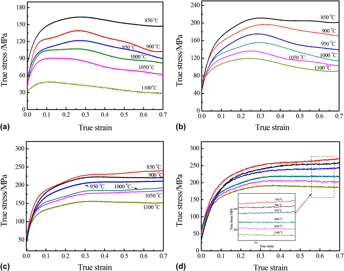
On the other hand, from Fig. 1, it can also be seen that the strain rate is a significant sensitive parameter for evaluating the trend of flow stress during plastic deformation, which reveals the work hardening tendency with an increasing strain rate. At the strain rate of 1 and 10 s−1, the work hardening and recovery of the specimens reach a dynamic equilibrium, which shows a steady state flow stress. This may be due to the restriction of dislocation movement and energy accumulation under lower temperature as well as shorter time. Nevertheless, higher temperature and low strain rate provide high mobility for nucleation and growth of DRX grains.
Thus, it can be concluded that DRX is more likely to happen at lower strain rate (0.01 and 1 s−1) and higher deformation temperature, whereas DRV occurs at relatively higher strain rate (1 and 10 s−1), especially under lower deformation temperature.
B. Deformation constitutive equation
Generally, the relationship between flow stress and deformation conditions can be analyzed via Arrhenius equation during hot deformation. Furthermore, Zener–Hollomon parameter (Z–H parameter), which was proposed by Zener and Hollomon in 1994, Reference Zener and Hollomon57 was a crucial hot working index and used to characterize the combined effect of temperature and strain rate on the flow stress behavior, which is expressed as follows:
 $$Z = \dot \varepsilon \cdot \exp \left[ {{Q \mathord{\left/ {\vphantom {Q {\left( {RT} \right)}}} \right. \kern-\nulldelimiterspace} {\left( {RT} \right)}}} \right] = f\left( \sigma \right)\quad ,$$
 $$\dot \varepsilon = {A_1}{\sigma ^{{n_1}}} \cdot \exp \left[ {{{ - Q} \mathord{\left/ {\vphantom {{ - Q} {\left( {RT} \right)}}} \right. \kern-\nulldelimiterspace} {\left( {RT} \right)}}} \right]\quad \alpha \sigma \lt 0.8\quad ,$$
 $$\dot \varepsilon = {A_2} \cdot \exp \left( {\beta \sigma } \right) \cdot \exp \left[ {{{ - Q} \mathord{\left/ {\vphantom {{ - Q} {\left( {RT} \right)}}} \right. \kern-\nulldelimiterspace} {\left( {RT} \right)}}} \right]\quad \alpha \sigma > 1.2\quad ,$$
 $$\dot \varepsilon = A{\left[ {\sinh \left( {\alpha \sigma } \right)} \right]^n} \cdot \exp \left[ {{{ - Q} \mathord{\left/ {\vphantom {{ - Q} {\left( {RT} \right)}}} \right. \kern-\nulldelimiterspace} {\left( {RT} \right)}}} \right]\quad {\rm{for}}\;{\rm{all}}\;\sigma \quad ,$$
where Z is the Zener–Hollomon parameter;
 $\dot \varepsilon$
is the strain rate (s−1); σ is the flow stress (MPa) for a given strain; Q is the deformation activation energy (kJ/mol); R is the gas constant [8.3145 J/(mol K)]; T is the deformation temperature (K); A
1, n
1, A
2, β, A, α, and n are the material constants, α ≈ β/n
1. Additionally, Eq. (2) is normally used to describe the creep deformation at low-stress level. In contrast, the exponential law description of Eq. (3) is suited to illustrate higher strain rate under high-stress level, while in Eq. (4) the hyperbolic sine law can be used for all deformation conditions.
1. Determination of strain-dependent material constants
Based on the above analysis, it can be found the flow stress curves experience different deformation stages under each value of strain. Furthermore, the functional relationship between strain and the material constants can be obtained in the constitutive equations. Therefore, the compensation of strain and coefficients relative to the material should be taken into account when deriving the constitutive equation. From Eqs. (2) and (3), the relationship between flow stress and strain rate are described as follows:
 $$\dot \varepsilon = A{\sigma ^{{n_1}}} \cdot \exp \left[ {{{ - Q} \mathord{\left/ {\vphantom {{ - Q} {\left( {RT} \right)}}} \right. \kern-\nulldelimiterspace} {\left( {RT} \right)}}} \right] = B{\sigma ^{{n_1}}}\quad \left( {{\rm{for}}\;{\rm{low}}\;{\rm{stress}}\;{\rm{level}}} \right)\quad ,$$
 $$\dot \varepsilon = A\exp \left( {\beta \sigma } \right) \cdot \exp \left[ {{{ - Q} \mathord{\left/ {\vphantom {{ - Q} {\left( {RT} \right)}}} \right. \kern-\nulldelimiterspace} {\left( {RT} \right)}}} \right] = B'\exp \left( {\beta \sigma } \right)\quad \left( {{\rm{for}}\;{\rm{high}}\;{\rm{stress}}\;{\rm{level}}} \right)\quad ,$$
where B and B′ are coefficients relative to the material, which are dependent on the deformation temperature.
According to Eqs. (5) and (6), we can obtain
 $$\ln \sigma = {1 \over {{n_1}}}\ln \dot \varepsilon - {1 \over {{n_1}}}\ln B\quad ,$$
 $$\sigma = {1 \over \beta }\ln \dot \varepsilon - {1 \over \beta }\ln B'\quad .$$
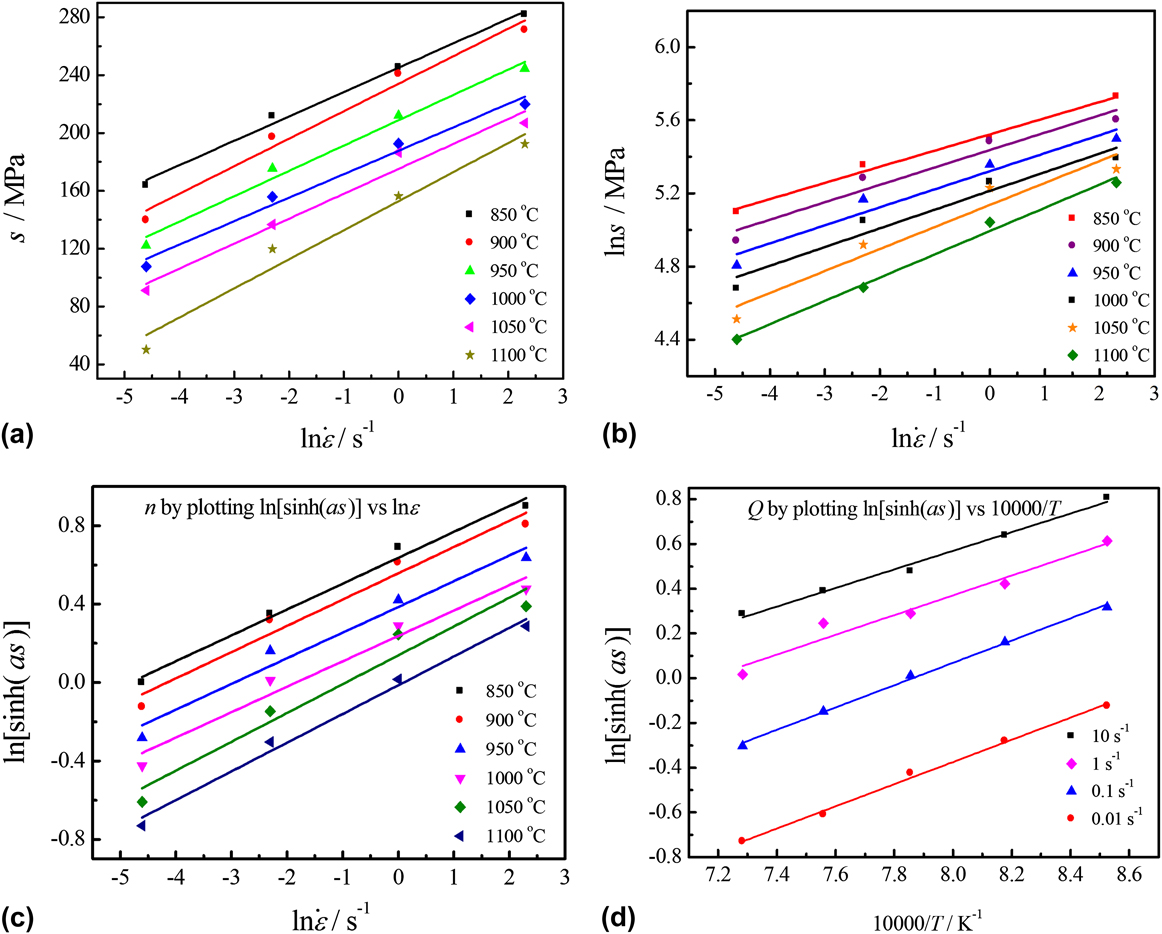
It is noticed that the values of n
1 and β can be respectively received from the reciprocals of the slopes of the lines in
 $\ln \sigma - \ln \dot \varepsilon$
and
 $\sigma - \ln \dot \varepsilon$
, as plotted in Figs. 2(a) and 2(b). Considering the slops of the lines at different temperatures is approximately same. Thus, the mean value of n
1 and β are calculated to be 9.68611 and 0.055781 MPa−1 by the linear fitting method, respectively. And α = β/n
1 = 0.0057 MPa−1.
Relationship between (a) σ and
 $\ln \dot \varepsilon$
; (b) ln σ and
 $\ln \dot \varepsilon$
; (c) ln[sinh(ασ)] and
 $\ln \dot \varepsilon$
; (d) ln[sinh(ασ)] and 10,000/T at different deformation conditions.
Equation (4) after differentiating can be re-written as:
 $$\ln \left[ {\sinh \left( {\alpha \sigma } \right)} \right] = \ln {{\dot \varepsilon } \mathord{\left/ {\vphantom {{\dot \varepsilon } n}} \right. \kern-\nulldelimiterspace} n} + {Q \mathord{\left/ {\vphantom {Q {\left( {nRT} \right)}}} \right. \kern-\nulldelimiterspace} {\left( {nRT} \right)}} - \ln {A \mathord{\left/ {\vphantom {A n}} \right. \kern-\nulldelimiterspace} n}\quad .$$
Base on Eq. (9), Q is calculated at a given strain rate as follows:
 $$Q = 10{\rm{,}}000nR{{\partial \left\{ {\left. {\ln \left[ {\sinh \left( {\alpha \sigma } \right)} \right]} \right\}} \right.} \over {\partial \left( {{{10{\rm{,}}000} \mathord{\left/ {\vphantom {{10{\rm{,}}000} T}} \right. \kern-\nulldelimiterspace} T}} \right)}}\quad .$$
Similarly, the values of 1/n and Q are calculated from the slops of lines in
 $\ln \left[ {\sinh \left( {\alpha \sigma } \right)} \right] - \ln \dot \varepsilon$
plot and ln[sinh(ασ)] − 1000/T plot [as shown in Figs. 2(c) and 2(d)], respectively. Hence, the mean values of n and Q are 5.286 and 383.64 KJ/mol. The value of ln A is determined from the interception of the same lines as Q. Then, by substituting the values of Q,
 $\dot \varepsilon$
, and T into Eq. (1), the value of Z can be calculated under different deformation conditions.
According to Eqs. (1) and (4), gives:
 $$Z = \dot \varepsilon \cdot \exp \left[ {{Q \mathord{\left/ {\vphantom {Q {\left( {RT} \right)}}} \right. \kern-\nulldelimiterspace} {\left( {RT} \right)}}} \right] = A{\left[ {\sinh \left( {\alpha \sigma } \right)} \right]^n}\quad .$$
Taking natural logarithm on both sides of Eq. (11), we can obtain
 $$\ln Z = \ln A + n\ln \left[ {\sinh \left( {\alpha \sigma } \right)} \right]\quad .$$
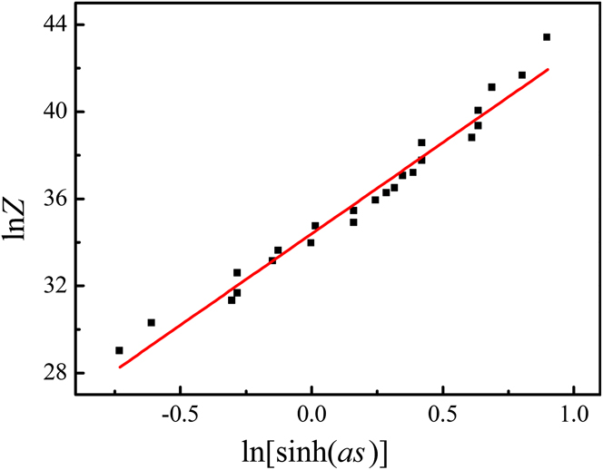
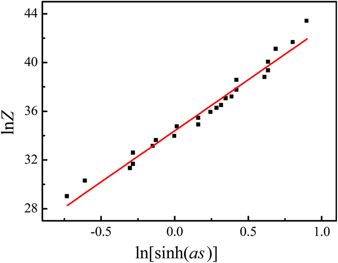
According to Eq. (12), the values of ln A and n are determined by the intercept and slope of ln Z − ln[sinh(ασ)] plot (as seen in Fig. 3) and the values are 34.37381, and 8.378, respectively.
Relationship between ln Z and ln[sinh(ασ)] for the experimental alloy.
2. Compensation of strain
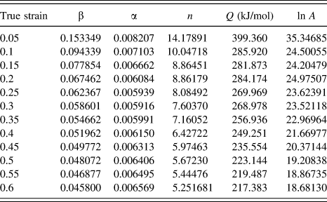
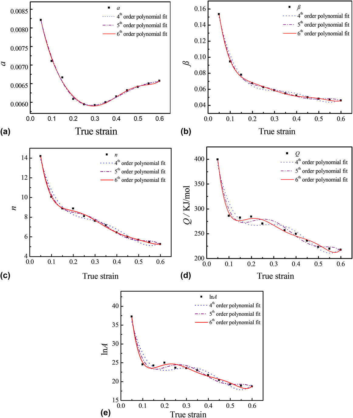
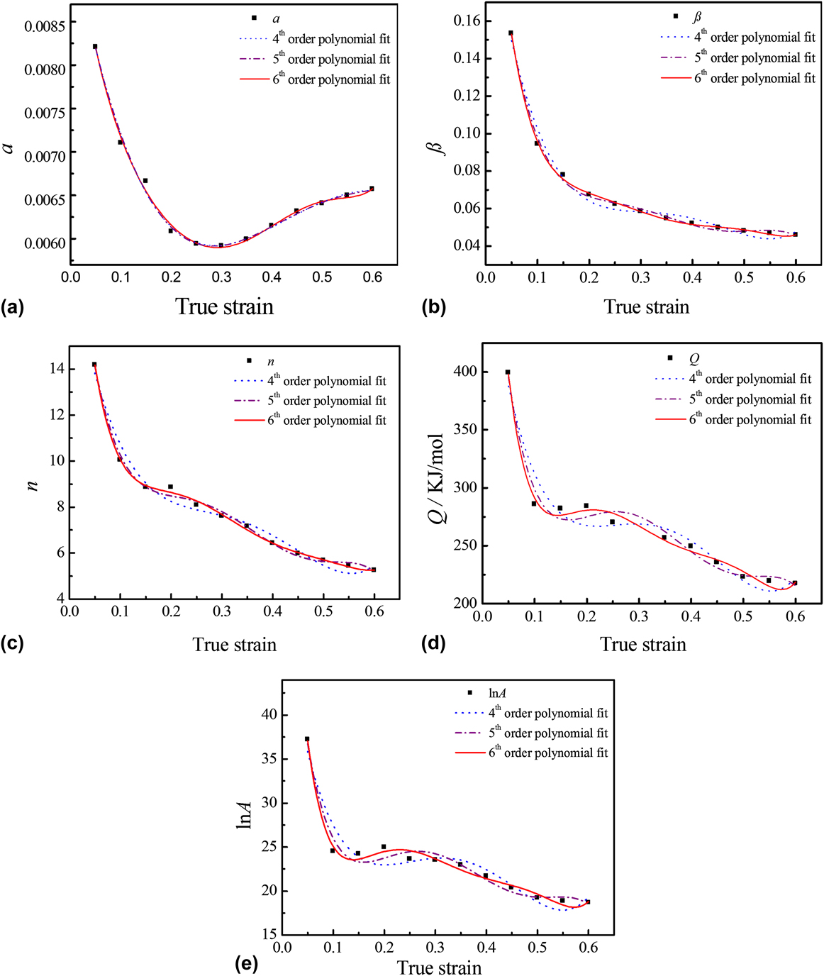
Most importantly, the values of α, β, n, Q, and ln A were calculated at various different strains with the range of 0.05–0.6, as displayed in Table I. Then, the polynomial fit was used to illustrate the effect of deformation strain on the material constants, as presented in Fig. 4. It can be seen that although the fourth or fifth order polynomial fit can reflect the trend of the curves, the sixth order polynomial fitting was more accurate and reliable. So the sixth polynomial fitting formulas are given in Eq. (13) and the corresponding polynomial coefficients are listed in Table II.
 $$\left\{ {\matrix{ {\alpha = {a_0} + {a_1}\varepsilon + {a_2}{\varepsilon ^2} + {a_3}{\varepsilon ^3} + {a_4}{\varepsilon ^4} + {a_5}{\varepsilon ^5} + {a_6}{\varepsilon ^6}} \hfill \cr {\beta = {b_0} + {b_1}\varepsilon + {b_2}{\varepsilon ^2} + {b_3}{\varepsilon ^3} + {b_4}{\varepsilon ^4} + {b_5}{\varepsilon ^5} + {b_6}{\varepsilon ^6}} \hfill \cr {n = {c_0} + {c_1}\varepsilon + {c_2}{\varepsilon ^2} + {c_3}{\varepsilon ^3} + {c_4}{\varepsilon ^4} + {c_5}{\varepsilon ^5} + {c_6}{\varepsilon ^6}} \hfill \cr {Q = {d_0} + {d_1}\varepsilon + {d_2}{\varepsilon ^2} + {d_3}{\varepsilon ^3} + {d_4}{\varepsilon ^4} + {d_5}{\varepsilon ^5} + {d_6}{\varepsilon ^6}} \hfill \cr {\ln A = {e_0} + {e_1}\varepsilon + {e_2}{\varepsilon ^2} + {e_3}{\varepsilon ^3} + {e_4}{\varepsilon ^4} + {e_5}{\varepsilon ^5} + {e_6}{\varepsilon ^6}} \hfill \cr} } \right.\quad .$$
Values of the material constants of Fe–36%Ni Invar alloy at different deformation strains.

Relationship between (a) α, (b) β, (c) n, (d) Q, (e) ln A.
Coefficients of the polynomial for α, β, n, Q, and ln A.

Combining with Eq. (11) and the definition of the hyperbolic law, the relationship between the flow stress and the Zener–Holloman parameter can be expressed as follows:
 $$\sigma = {1 \over \alpha }\ln \left\{ {{{\left( {{Z \over A}} \right)}^{1{\rm{/}}n}} + {{\left[ {{{\left( {{Z \over A}} \right)}^{2{\rm{/}}n}} + 1} \right]}^{1/2}}} \right\}\quad .$$
Finally, the modified constitutive equations considering the compensation of strain, which can accurately predict the flow at different strains, are given as follows:
 $$\left\{ {\matrix{ {Z = \dot \varepsilon \cdot \exp \left[ {{Q \mathord{\left/ {\vphantom {Q {\left( {RT} \right)}}} \right. \kern-\nulldelimiterspace} {\left( {RT} \right)}}} \right]} \hfill \cr {\alpha = 0.00998 - 0.04724\varepsilon + 0.28001{\varepsilon ^2} - 1.14957{\varepsilon ^3}} \hfill \cr{ + 2.98287{\varepsilon ^4} - 4.02328{\varepsilon ^5} + 2.11567{\varepsilon ^6}} \hfill \cr {\beta = 0.29325 - 4.08492\varepsilon + 31.28468{\varepsilon ^2} - 126.56914{\varepsilon ^3}} \hfill \cr { + 277.30693{\varepsilon ^4} - 311.02551{\varepsilon ^5} + 139.8852{\varepsilon ^6}} \hfill \cr {n = 25.37963 - 335.47325\varepsilon + 2732.81246{\varepsilon ^2} - 11{\rm{,}}298.70967{\varepsilon ^3}} \hfill \cr { + 24{\rm{,}}560.11807{\varepsilon ^4} - 26{\rm{,}}948.30984{\varepsilon ^5} + 11{\rm{,}}796.69012{\varepsilon ^6}} \hfill \cr {Q = 746.02588 - 10{\rm{,}}875.25889\varepsilon + 97{\rm{,}}579.63903{\varepsilon ^2} - 432{\rm{,}}386.1054{\varepsilon ^3}} \hfill \cr { + 1{\rm{,}}004{\rm{,}}500{\varepsilon ^4} - 1{\rm{,}}177{\rm{,}}440{\varepsilon ^5} + 549{\rm{,}}513.162{\varepsilon ^6}} \hfill \cr {\ln A = 76.08817 - 1216.7817\varepsilon + 10{\rm{,}}836.56145{\varepsilon ^2} - 47{\rm{,}}344.54483{{\rm{\varepsilon }}^3}} \hfill \cr { + 10{\rm{,}}8431.48162{\varepsilon ^4} - 125{\rm{,}}471.09034{\varepsilon ^5} + 57{\rm{,}}912.20005{\varepsilon ^6}} \hfill \cr {\sigma = {1 \over \alpha }\ln \left\{ {{{\left( {{Z \over A}} \right)}^{1{\rm{/}}n}} + {{\left[ {{{\left( {{Z \over A}} \right)}^{2{\rm{/}}n}} + 1} \right]}^{1/2}}} \right\}} \hfill \cr} } \right.\quad .$$
3. Verification of the modified constitutive equation
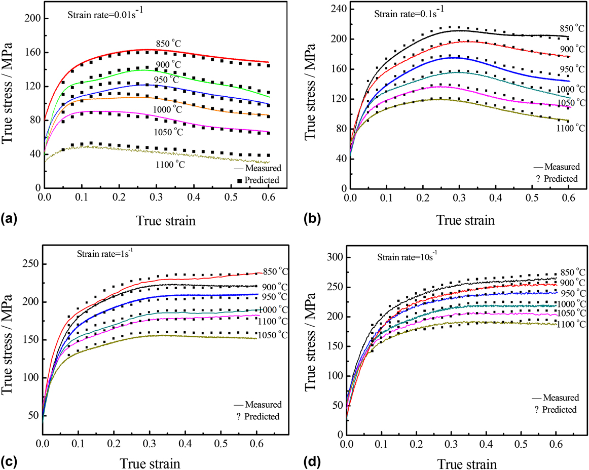
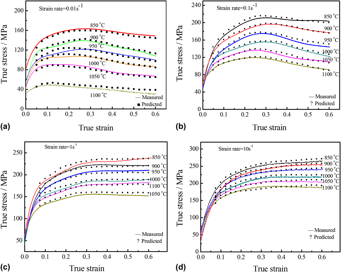
To confirm the accuracy of modified constitutive equation of Fe–36%Ni Invar alloy at elevated temperature, comparison between the calculated flow stress values and the experimental flow stress plots are shown in Fig. 5. It can be seen that the deviation between the calculated and measured flow stress values at strain rates from 0.01 to 10 s−1 as well as deformation temperatures from 850 to 1100 °C are very small. In other words, the proposed deformation constitutive equation can be used to accurately estimate the flow stress, which also provides some closely related information about the metal forming process. Thereby, the modified constitutive equation can quantify its predictability by virtue of standard statistical parameters such as correlation coefficient R and average absolute relative error AARE, which is expressed as follows:
 $$R = {{\sum\limits_{i = 1}^N {\left( {{E_i} - \bar E} \right)\left( {{P_i} - \bar P} \right)} } \over {\sqrt {\sum\limits_{i = 1}^N {{{\left( {{E_i} - \bar E} \right)}^2}} \sum\limits_{i = 1}^N {{{\left( {{P_i} - \bar P} \right)}^2}} } }}\quad ,$$
 $${\rm{AARE}}\left( \% \right) = {1 \over N}\sum\limits_{i = 1}^N {\left| {{{{E_i} - {P_i}} \over {{E_i}}}} \right| \times 100} \quad ,$$
where E is the experimental value; P is the predicted value obtained from the modified constitutive equation;
 $\bar E$
and
 $\bar P$
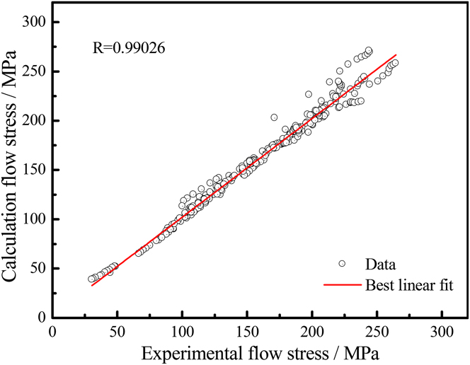
is the mean values of M and P, respectively. N is the total number of data points applied in the calculation. The linear relationship between the experimental and predicted flow stress values are presented in Fig. 6.
Comparison between the predicted and experimental flow stress from the modified constitutive equation at the temperature of 850–1100 °C with the strain rates of (a) 0.01 s−1; (b) 0.1 s−1; (c) 1 s−1; (d) 10 s−1.
Correlation between the experimental and calculated flow stress values obtained from the modified constitutive equation.
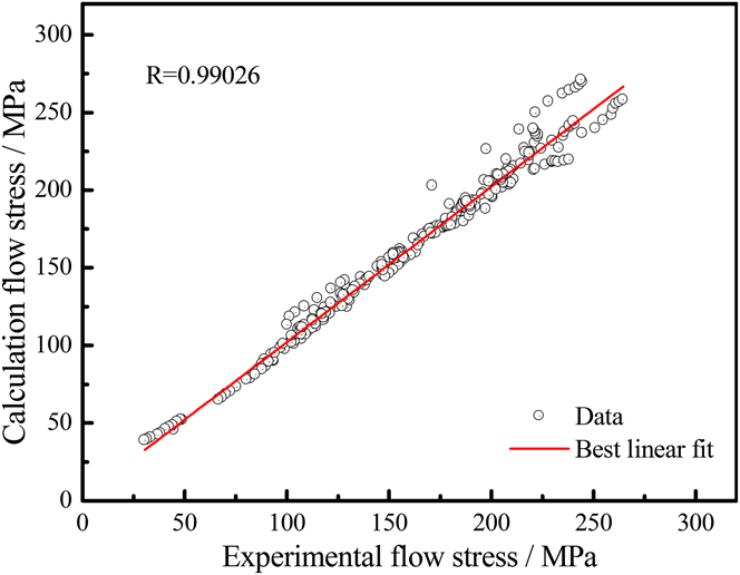
It is widely admitted that R value is used to explain the relevance of the linear fitting between the experimental and predicted data, while the AARE is computed via a term by term comparison of the relative error. Therefore, the AARE is more reliable to predict the accuracy of the modified constitutive equation. As shown in Fig. 6, the values of R and AARE are found to be 99.026% and 3.94%, respectively. In concrete terms, these statistical analyses can verify the accuracy and reliability of the modified constitutive equation at deformation conditions for the Fe–36%Ni Invar alloy.
4. Zener–Holloman parameter map
As mentioned above, the temperature and strain rate are two crucial factors to experimental materials during hot deformation. From Eq. (1), it can be seen that the effects of deformation temperature and strain rate are combined by Z–H parameter. Therefore, combined Z–H parameter and the modified constitutive equation, Z–H parameter map can be established at a given strain to exhibit the connection between temperatures and strain rates, and evaluated the extent of DRX. Reference Marandi, Zarei-Hanzaki, Haghdadi and Eskandari21,Reference Feng, Zhang, Liu and Deng42,Reference Bobbili and Madhu43
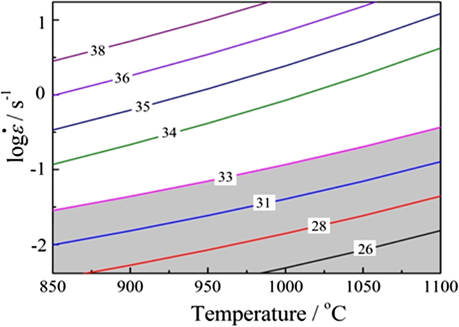
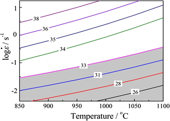
Figure 7 illustrates that the deformation temperatures in the range of 850–1100 °C and the strain rates of 0.01–10 s−1 have prominent influence on Z–H parameter. It is noted from the map that contour numbers denote the value of ln Z and shaded region represents the occurrence of DRX behavior at a strain of 0.7. Furthermore, the value of ln Z declines steadily with increase in temperature or decrease in strain rate. Most importantly, according to the Z–H parameter map, it can be concluded that the DRX behavior of deformed specimens are more likely to take place when the ln Z is <33 s−1 and the Z–H parameter peaks at 850 °C, 10 s−1. The lower the values of ln Z the more easily DRX may occur, which means large extent of dynamic softening happened.
Z–H parameter map at the strain of 0.7. Contour numbers presents the values of ln Z.
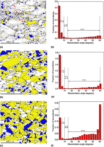
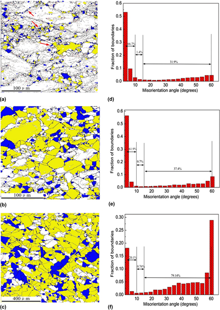
With the help of electron backscattered diffraction (EBSD) technique, Figs. 8(a)–8(c) further reveal the proportion of recrystallized and the sub-structured grains distinctly increased with the decrease of ln Z value and the increase of temperature. This phenomenon exhibits that the higher deformation temperature provided more energy, which was beneficial in the nucleation and growth of recrystallized grain. The red arrows in Fig. 8(a) show that new recrystallized grains occurred at the intensive area of low angle grain boundaries (LAGBs) at 850 °C. Combined with Figs. 8(d)–8(f), we find that with the value of ln Z dropped from 30.9 to 24.3, the frequency of LAGBs decreased from 66.7 to 20.1% and high angle grain boundaries (HAGBs) increased from 31.9 to 79.14%, while the medium angle grain boundaries (MAGBs) only marginally declined. It can be inferred that during this deformation process, a large fraction of LAGBs would merge and be converted into HAGBs, which was a noticeable feature of continuous DRX. Reference Yin, Park, Li, Ye, Zuo, Lee, Yeom and Mi58,Reference Sakai, Belyakov, Kaibyshev, Miura and Jonas59 So to some extent, the analysis of microstructure evolution verified the accurate estimation of Z–H parameter map.
EBSD analyses the microstructures and grain boundaries misorientation angles at a strain rate of 0.01 s−1 at deformed conditions of (a), (d) 850 °C, ln Z = 30.9 s−1; (b), (e) 950 °C, ln Z = 28.6 s−1; (c), (f) 1100 °C, ln Z = 24.3 s−1. The fully recrystallized, sub-structured, and deformed grains are revealed with blue, yellow, and white colors, respectively. The low angle grain boundaries (misorientation between 2° and 10°), medium angle grain boundaries (misorientation between 10° and 15°) and high angle grain boundaries (misorientation more than 15°) are shown as gray, red, and black lines, respectively.

IV. CONCLUSION
-
(1) The flow stress of Fe–36%Ni Invar alloy enhanced with the increasing of strain rate and the decreasing of deformation temperature, which can be displayed by Zener–Hollomon parameter in Arrhenius type equation.
-
(2) The constitutive analysis illustrated that strain has significant effect on the flow stress, material constants (i.e., α, β, n, and ln A) and hot deformation activation energy (Q). Then, sixth order polynomial fit method significantly optimized the relationship between the compensation of strain and material constants, hot deformation activation energy.
-
(3) The modified constitutive equation can accurately and reliably predict the flow stress by the average absolute relative error (AARE was found to be 99.026%) in the hot deformation conditions.
-
(4) According to the Z–H parameter map, the value of ln Z declined steadily with increase in temperature or decrease in strain rate. Additionally, it can be concluded that the DRX behavior were more likely to occur when the ln Z is <33 s−1.
ACKNOWLEDGMENT
This work was supported by the National Key Research Project of China (2016YFB0300402).