1. Introduction
The global dynamics of flows past axisymmetric bluff bodies at moderate Reynolds numbers is now fairly well established, both experimentally and numerically. In this regard, previous investigations have been mainly carried out for the wake flows around a sphere (Taneda Reference Taneda1956; Magarvey & Bishop Reference Magarvey and Bishop1961b
; Roos & Willmarth Reference Roos and Willmarth1971; Nakamura Reference Nakamura1976; Natarajan & Acrivos Reference Natarajan and Acrivos1993; Johnson & Patel Reference Johnson and Patel1999; Ormières & Provansal Reference Ormières and Provansal1999; Ghidersa & Dušek Reference Ghidersa and Dušek2000; Gumowski et al. Reference Gumowski, Miedzik, Goujon-Durand, Jenffer and Wesfreid2008; Pier Reference Pier2008), bullet-shaped bodies (Sanmiguel-Rojas et al. Reference Sanmiguel-Rojas, Sevilla, Martínez-Bazán and Chomaz2009, Reference Sanmiguel-Rojas, Jiménez-González, Bohorquez, Pawlak and Martínez-Bazán2011; Bohorquez et al. Reference Bohorquez, Sanmiguel-Rojas, Sevilla, Jiménez-González and Martínez-Bazán2011), discs (Fabre, Auguste & Magnaudet Reference Fabre, Auguste and Magnaudet2008; Meliga, Chomaz & Sipp Reference Meliga, Chomaz and Sipp2009; Szaltys et al. Reference Szaltys, Chrust, Przadka, Goujon-Durand, Tuckerman and Wesfreid2012; Bobinski, Goujon-Durand & Wesfreid Reference Bobinski, Goujon-Durand and Wesfreid2014), spheroids (Mittal Reference Mittal1999; Chrust, Bouchet & Dušek Reference Chrust, Bouchet and Dušek2010) and hemispheres (Kim & Choi Reference Kim and Choi2003) (for a comprehensive review please refer to Ern et al. Reference Ern, Risso, Fabre and Magnaudet2012). These studies have revealed that the sequence of transitions which occur with increasing values of the Reynolds number differs in a subtle manner among these bluff bodies. The first bifurcation is a stationary one associated with a pair of counter-rotating azimuthal modes for azimuthal wavenumber
 $m = \pm 1$
. As the Reynolds number increases, a second transition/bifurcation occurs, leading to the formation of a hairpin-shaped vortex structure from double-threaded vortex structures. This second transition is known as the secondary bifurcation, which is unsteady. In the case of spheres and bullet-shaped bluff bodies, the wake is planar symmetric, which is conserved in the unsteady time-periodic regime up to a certain Reynolds number. However, in the wake of a hemisphere and of thin discs, the secondary oscillatory bifurcation does not preserve the symmetry plane (Ern et al. Reference Ern, Risso, Fabre and Magnaudet2012). Furthermore, the errors in the predictions made by the global linear stability analysis performed on axisymmetric base flows with non-axisymmetric ones vary greatly among these geometries. For instance, in the case of spheres and thin discs, the critical Reynolds number at which the transition from a steady non-axisymmetric wake to periodic vortex shedding occurs is in remarkable agreement between both the approaches whereas, for bullet-shaped bodies, the error is substantially higher (Bohorquez et al. Reference Bohorquez, Sanmiguel-Rojas, Sevilla, Jiménez-González and Martínez-Bazán2011). This can be attributed to the relative difference of the critical Reynolds numbers corresponding to the primary and secondary bifurcations,
 $\varDelta =(Re_{c2}-Re_{c1})/Re_{c1}$
(Fabre et al. Reference Fabre, Auguste and Magnaudet2008; Bohorquez et al. Reference Bohorquez, Sanmiguel-Rojas, Sevilla, Jiménez-González and Martínez-Bazán2011); here,
 ${\textit{Re}}_{c1}$
and
 ${\textit{Re}}_{c2}$
denote the critical Reynolds number corresponding to the primary and secondary bifurcations, respectively. If
 $\varDelta$
is much less than 1, the global stability analysis considering the axisymmetric steady base flow can closely predict
 ${\textit{Re}}_{c2}$
(Bohorquez et al. Reference Bohorquez, Sanmiguel-Rojas, Sevilla, Jiménez-González and Martínez-Bazán2011). This condition closely holds good for thin discs, a sphere, and a bullet-shaped body with unit aspect ratio, but fails to do so for blunt-shaped slender bodies, and ellipsoids with large aspect ratios (see figure 14 in Bohorquez et al. Reference Bohorquez, Sanmiguel-Rojas, Sevilla, Jiménez-González and Martínez-Bazán2011, for an example). The present study aims to address the above aspect by studying the stability and dynamics of flows past bubble-shaped bluff-bodies, modelled as spherical and elliptical caps, both numerically and experimentally.
The transition scenarios arising in bluff-body wakes were first qualitatively revealed by the experimental studies carried out on immiscible drops (Magarvey & Bishop Reference Magarvey and Bishop1961a
,
Reference Magarvey and Bishopb
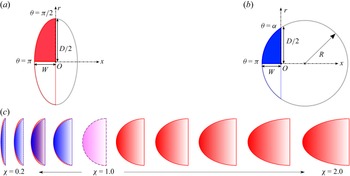
) and liquid-filled spheres (Magarvey & MacLatchy Reference Magarvey and MacLatchy1965) falling in water. By choosing density ratios between the fluids such that the bodies underwent only tiny displacements, they were able to qualitatively describe the first two bifurcation states arising in the flow past a rigid sphere. In the case of falling drops, the presence of surface-active impurities at the liquid–liquid interface ensured that they stayed in a semi-rigid spherical shape, thereby allowing a qualitative comparison with flows past rigid bodies. These were further extended and corroborated by Nakamura (Reference Nakamura1976). Similar qualitative comparisons have also been made from studies carried out on freely rising axisymmetric bodies such as bubbles and spheroids (Magnaudet & Mougin Reference Magnaudet and Mougin2007; Ern et al. Reference Ern, Risso, Fabre and Magnaudet2012). The bubble dynamics is indeed more complicated than that of solid bodies (Fernandes et al. Reference Fernandes, Risso, Ern and Magnaudet2007; Cano-Lozano et al. Reference Cano-Lozano, Tchoufag, Magnaudet and Martínez-Bazán2016; Bonnefis et al. Reference Bonnefis, Sierra-Ausin, Fabre and Magnaudet2024). Using both experimental and numerical methods, it has been established that the shape fluctuations do not play a significant role in the regime of path oscillations of bubbles rising in clean water (Ellingsen & Risso Reference Ellingsen and Risso2001; Mougin & Magnaudet Reference Mougin and Magnaudet2001). The aspect ratio of the bubble remains the same after the initial transients, with the bubble attaining a terminal shape and velocity. Studying the wake of fixed axisymmetric bodies is a necessary step towards understanding the characteristics observed in the aforementioned systems (Ern et al. Reference Ern, Risso, Fabre and Magnaudet2012). Figure 1 shows the experimentally observed axisymmetric bubble-shape configurations considered in the present work, which are modelled as spherical and elliptical caps. The geometries are characterised by the aspect ratio
 $\chi$
, which is defined as the ratio of the height of the bubble (measured in the direction parallel to the revolution axis) and the radius of its base. The aspect ratio is varied in the range
 $0.2 \leqslant \chi \leqslant 2$
, which qualitatively corresponds to the different shapes observed for a bubble rising in quiescent fluid. To our knowledge, such bubble-shaped solid bodies of intermediate shape have not been studied yet, and it is expected that their wakes will also present specific features, which are worth investigating experimentally and numerically.
Present shapes of bluff bodies inspired from our previous work on rising bubbles which are available as APSDFD2020 video (Muniyammal, Mandal & Kumar Reference Muniyammal, Mandal and Kumar2020). These are modelled here as (a) spherical and (b) elliptical caps. The dotted lines correspond to (a)
 $\chi = 0.6$
and (b)
 $\chi = 0.8$
.

It is by now well established that the wakes of axisymmetric bluff bodies are characterised by a region of absolute instability, the spatial extent of which, interestingly, closely follows the toroidal recirculating region downstream of the bluff body (Chomaz Reference Chomaz2005; Pier Reference Pier2008; Meliga et al. Reference Meliga, Chomaz and Sipp2009). It has been shown that the recirculation zone could be viewed as an effective wave maker, with the pocket of absolute instability within it fixing the global shedding frequency (Monkewitz Reference Monkewitz1988; Pier Reference Pier2008; Meliga et al. Reference Meliga, Chomaz and Sipp2009). Furthermore, as the onset of instability is related to the amount of vorticity generated at the body’s surface, a relevant velocity scale to characterise this downstream vortex is the maximum reverse-flow velocity on its axis (Fernandes et al. Reference Fernandes, Risso, Ern and Magnaudet2007; Magnaudet & Mougin Reference Magnaudet and Mougin2007). By defining a modified Reynolds number based on the recirculation length,
 $L_{ {r}}$
, and the maximum of the reverse-flow velocity,
 $U_{\textit{rev}}$
, Fernandes et al. (Reference Fernandes, Risso, Ern and Magnaudet2007) have shown that the dimensional amplitudes and frequencies observed in freely rising axisymmetric bodies are independent of the body shape. Although the flow structures observed in plane wakes past two-dimensional symmetric bluff bodies are qualitatively different, it has been shown recently that
 $L_{ {r}}$
and
 $U_{\textit{rev}}$
are indeed the relevant length and velocity scales to describe the primary instability (Chiarini, Quadrio & Auteri Reference Chiarini, Quadrio and Auteri2022). The predicted scaling law has been shown to be robust and holds for planar wakes corresponding to differently shaped geometries. The choice of the velocity scale was attributed to the fact that the spatial location corresponding to
 $U_{\textit{rev}}$
is the region associated with the largest axial shear (Hammond & Redekopp Reference Hammond and Redekopp1997). As reverse flow enhances the growth of disturbances travelling upstream of the absolutely unstable region (Monkewitz Reference Monkewitz1988), the choice of
 $L_{ {r}}$
and
 $U_{\textit{rev}}$
as the relevant scales indeed seem pertinent. Indeed, as the vortex shedding from axisymmetric bodies is different from planar bodies as it is sensitive to the shape of the bluff body and the nature of separation on the body (Monkewitz Reference Monkewitz1988), it is worthwhile examining the validity of the existing scaling laws. We show that the critical Reynolds number corresponding to the primary bifurcation remains independent of the aspect ratio when scaled by
 $L_{ {r}}$
and
 $U_{\textit{rev}}$
.
The main objective of the present work is to examine the flow regimes taking place in the laminar wake of axisymmetric bluff bodies, modelled as spherical and elliptical caps. By combining flow visualisations and particle-image-velocimetry techniques, and global stability analyses, we investigate the following: (a) whether the aspect ratios for which the critical Reynolds numbers predicted using axisymmetric base flow fields are in agreement with the experimental observations made using dye visualisations and particle-image-velocimetry techniques; (b) whether the reported scaling laws on planar wakes past bluff bodies (Chiarini et al. Reference Chiarini, Quadrio and Auteri2022), based on maximum reverse-flow velocity and the recirculation length, hold for flows past axisymmetric geometries; (c) and we qualitatively provide insight into the symmetry preserving/breaking nature of flows past axisymmetric bodies using dye visualisations and particle image velocimetry. The observed findings are in excellent agreement with the available literature on flow past a hemisphere (
 $\chi = 1$
) (Kim & Choi Reference Kim and Choi2003; Jiménez-González et al. Reference Jiménez-González, Manglano-Villamarín and Coenen2019), and with the wake of a blunt-shaped cylindrical body with a rounded ellipsoidal nose (
 $\chi = 2$
) (Bohorquez et al. Reference Bohorquez, Sanmiguel-Rojas, Sevilla, Jiménez-González and Martínez-Bazán2011).
To this end, the paper is organised as follows. The geometrical configurations, the numerical methods and the experimental techniques used in the present study are described in § 2. The base flow characteristics and the results from the global linear stability analyses for geometries with varying aspect ratios are discussed in detail in § 3. Comparisons of the numerically obtained results with experimental observations using flow visualisation and particle-image-velocimetry techniques are presented in § 4. The article ends with concluding remarks in § 5.
2. Methodology
2.1. Geometry
The geometrical configurations considered in the present study are based on the shapes observed as a bubble rises through a quiescent liquid (see figure 1). The shape of the rising bubble can vary greatly depending on the solutal composition of the surrounding liquid, or indeed as it passes through a liquid–liquid interface (figure 1
b). The bubble shape is modelled as an elliptical cap, and as a spherical cap with a flat circular base. These are shown in figure 2 in panels (a) and (b), respectively. The shapes are characterised by the diameter of the circular base
 $D$
, and by the width (or height) of the bubble
 $W$
. The varying shapes can be geometrically characterised by the aspect ratio
 $\chi = W/(D/2)$
, as shown in figure 2(c).
Schematic of the geometrical configurations. Bubble-shaped bluff bodies modelled as an (a) elliptical cap, and (b) as a spherical cap. (c) Comparison of the two different configurations with increasing aspect ratio, with the spherical cap denoted by dashed blue lines, and the elliptical cap by solid red lines. The spherical cap shapes were considered within the range of aspect ratios
 $0.2 \leqslant \chi \leqslant 1$
whereas the bubble surface modelled as an elliptical cap extends up to
 $\chi = 2$
. The case of a hemisphere corresponds to
 $\chi = 1$
.

From the axisymmetry of the geometrical configuration a cylindrical coordinate system has been used for global linear stability analysis investigation with
 $r$
,
 $\theta$
and
 $x$
denoting radial, azimuthal and axial coordinates respectively. The
 $x$
-axis is aligned with the free-stream velocity, with the origin at the centre of the circular base, as shown in figure 2. The bubble surfaces modelled as elliptical caps are defined by the following parametric equations:
 \begin{equation} x = W \cos \theta , \quad \quad r = \frac {D}{2} \sin \theta , \end{equation}
with
 $\theta$
varying from
 $\pi$
to
 $\pi /2$
. The spherical cap on the other hand is defined based on the sphere of which it forms a part, as
 \begin{eqnarray} x = (R-W) + R \cos \theta , \quad \quad r= R \sin \theta , \end{eqnarray}
with
 $R$
being the radius of the sphere, and
 $\theta$
denoting an angle varying between
 $\pi$
and the desired angle
 $\alpha$
. These are given by
 \begin{eqnarray} R = \frac {(D^2/4 + W^2)}{2 W}, \,\,\,\, \tan \alpha = \frac {D/2}{(R - W)}. \end{eqnarray}
It is to be noted that the bubble shape modelled as a spherical cap corresponds to a part of a sphere, and beyond
 $\chi \gt 1$
the maximum diameter exceeds the base diameter
 $D$
. To this end the aspect ratios were varied within the range
 $0.2 \leqslant \chi \leqslant 1$
for the spherical cap, and
 $0.2 \leqslant \chi \leqslant 2$
for the elliptical cap.
2.2. Governing equations
The governing equations are the Navier–Stokes equations. Here, we consider these equations for an incompressible axisymmetric flow in the cylindrical coordinate system
 $(x, r, \theta )$
for a fluid with density
 $\rho$
and dynamic viscosity
 $\mu$
. The characteristic length, time, velocity and pressure scales are considered as
 $D$
,
 $D/U_{\infty }$
,
 $U_{\infty }$
and
 $\rho U_{\infty }^2$
, respectively. With these scales, the non-dimensional forms of the governing equations are given as follows:
 \begin{align} \partial _t \boldsymbol {u} + (\boldsymbol {u} \boldsymbol{\cdot }\boldsymbol{\nabla })\boldsymbol {u} &= - \boldsymbol{\nabla }p + \frac {1}{Re} {\nabla} ^2 \boldsymbol {u} , \end{align}
 \begin{align} \boldsymbol{\nabla }\boldsymbol{\cdot }\boldsymbol {u} &= 0. \end{align}
Here,
 ${\textit{Re}} = \rho U_{\infty } D / \mu$
is the Reynolds number,
 $\boldsymbol{u}$
(
 $u_x , u_r , u_{\theta }$
) is velocity vector and p is the pressure. These equations are solved in the axisymmetric coordinate system keeping the origin at the centre of the base, as schematically shown in figure 3(a). The computational domain,
 $\varOmega$
, is shown in figure 3(b). We used the following boundary conditions to solve the above equations. At the inlet boundary (
 $\partial \varGamma _{{\textit{in}}}$
), a uniform axial velocity
 $\boldsymbol{u} = (U_{\infty }, 0, 0)$
was prescribed. A no-slip condition (
 $\boldsymbol{u} = 0$
) was enforced on the model surface (
 $\partial \varGamma _{{\textit{body}}}$
). A no-stress condition was imposed at the outlet (
 $\partial \varGamma _{{\textit{out}}}$
), while a free-slip condition is applied at the far-field boundary (
 $\partial \varGamma _{\textit{far}}$
). The resulting velocity field from this simulation is used as the initial guess for the computation of the base flow. The base flow field (
 $\overline {u}_{x}, \overline {u}_r, \overline {u}_\theta$
and
 $\overline {p}$
) was calculated using the steady equations,
 \begin{align} (\boldsymbol{\overline {u}}.\boldsymbol{\nabla })\boldsymbol{\overline {u}} &= - \boldsymbol{\nabla }\bar {p} + \frac {1}{Re} {\nabla} ^2 \boldsymbol{\overline {u}}, \end{align}
 \begin{align} \boldsymbol{\nabla }. \boldsymbol{\overline {u}} &= 0, \end{align}
Sketch of the body and the computational domain in the
 $x,r,\theta$
coordinate system. The axial direction
 $x$
is aligned with the free-stream velocity
 $U_{\infty }$
, with the origin at the centre of the circular base of diameter
 $D$
(a). The domain boundaries are denoted as
 $\partial \varGamma _{{\textit{in}}}$
(inlet),
 $\partial \varGamma _{{\textit{out}}}$
(outlet),
 $\varGamma _{\textit{far}}$
(upper) and
 $\partial \varGamma _{{\textit{body}}}$
(body) (b). The mesh in the computational domain is shown in (c).

with similar boundary conditions discussed above for (2.4).
The stability analysis of the above base flow was performed by superimposing an infinitesimal(
 $\epsilon$
) three-dimensional perturbation
 $(\boldsymbol{u}^{\prime }, p^{\prime })$
on the base flow field, i.e.
 $(u_{x}, u_r,u_\theta ,p) = (\overline {u}_x,\overline {u}_r,\overline {u}_\theta ,\overline {p}) + \epsilon (u^{\prime }_x, u^{\prime }_r, u^{\prime }_\theta , p^{\prime })$
. The evolution of these perturbations is governed by the linearised Navier–Stokes equations
 \begin{align} \frac {\partial \boldsymbol {u}^{\prime }}{\partial t} + (\boldsymbol{\overline {u}}.\boldsymbol{\nabla })\boldsymbol {u}^{\prime } + (\boldsymbol {u}^{\prime }.\boldsymbol{\nabla }) \boldsymbol{\overline {u}} &= -\boldsymbol{\nabla }p^{\prime } + \frac {1}{Re} {\nabla} ^2 \boldsymbol {u}^{\prime }, \end{align}
 \begin{align} \boldsymbol{\nabla }. \boldsymbol {u}^{\prime } &= 0. \end{align}
These equations were converted to an eigenvalue problem by considering the following normal-mode form of the perturbations:
 \begin{eqnarray} [\boldsymbol{u}^{\prime }, p^{\prime }](r, \theta , x, t) = [\hat {u}_r,\hat {u}_{\theta },\hat {u}_{x},\hat {p}](r,x)e^{\dot {\imath }m\theta + \lambda t} + \textrm{c.c}, \end{eqnarray}
where
 $\textrm{c.c}$
denotes complex conjugate,
 $m \in \mathbb{R}$
is the azimuthal mode number and
 $\lambda = \sigma + \dot {\imath }\omega$
is the complex eigenfrequency. The growth rate and the circular frequency are given by
 $\sigma$
and
 $\omega$
, respectively. The perturbations are stationary when
 $\omega = 0$
and oscillatory when
 $\omega \neq 0$
.
Substituting the normal-mode form (2.7) in the linearised Navier–Stokes equations ((2.6a ) and (2.6b )), one can get a generalised eigenvalue problem of the form
 \begin{eqnarray} \boldsymbol{A} \boldsymbol{\hat {u}} + \lambda \boldsymbol{B} \boldsymbol{\hat {u}} = 0, \end{eqnarray}
where
 $\boldsymbol{\hat {u}} = [\hat {u}_x,\hat {u}_r,\hat {u}_\theta ,\hat {p}]$
is a vector consisting of the shape functions;
 $\boldsymbol{A}$
and
 $\boldsymbol{B}$
can be called the stiffness and mass matrices, in the context of the finite element method. However, (2.8) is an eigenvalue problem which was solved using the shift-invert Arnoldi technique, with the following boundary conditions:
 \begin{align} \hat {u}_x = \hat {u}_r = \hat {u}_\theta &= 0 & on\,\,\,&\partial \varGamma _{{\textit{body}}} \nonumber, \\ \hat {u}_x = \hat {u}_r = \hat {u}_\theta &= 0 & on\,\,\,&\partial \varGamma _{{\textit{in}}} \nonumber, \\ \hat {u}_r = \partial _r \hat {u}_x = \partial _r\hat {u}_\theta &= 0 & on\,\,\,&\partial \varGamma _{{\textit{top}}} \nonumber, \\ -\hat {p}\boldsymbol{n} + {\textit{Re}}^{-1} (\boldsymbol{\nabla }\boldsymbol{\hat {u}} + \boldsymbol{\nabla }\boldsymbol{\hat {u}}^{T})\,\cdot\,\boldsymbol{n} &= 0 & on\,\,\,&\partial \varGamma _{{\textit{out}}}. \end{align}
On the axis
 $\partial \varGamma _{{axis}}$
boundary conditions are specified based on the azimuthal mode number
 $m$
:
 $\hat {u}_r = \partial _{r}\hat {u}_{x} = \partial _{r}p = 0$
for
 $m = 0$
;
 $\partial _{r}\hat {u}_r = \partial _{r}\hat {u}_{\theta } = \hat {u}_{x} = \hat {p} = 0$
for
 $\vert m \vert = 1$
; and
 $\hat {u}_{r} = \hat {u}_{\theta } = \hat {u}_{x} = \hat {p} = 0$
for
 $\vert m \vert \geqslant 2$
.
2.3. Numerical details for stability calculations
The axisymmetric base flow fields and the generalised eigenvalue problem were solved numerically using the open-source software FreeFEM++ (http://www.freefem.org). The unknown velocity and pressure fields were spatially discretised using Taylor–Hood finite elements, specifically
 $P_2$
elements for velocity components and
 $P_1$
elements for pressure. Mesh generation and matrix assembly were carried out using FreeFEM++ (see Gopalakrishnan Reference Gopalakrishnan2014 for implementation details). The base flow was computed following a procedure similar to that outlined in Marquet, Sipp & Jacquin (Reference Marquet, Sipp and Jacquin2008) and Gopalakrishnan, Pier & Biesheuvel (Reference Gopalakrishnan, Pier and Biesheuvel2014). Initially, a time-marching direct numerical simulation (DNS) of the Navier–Stokes equations (2.4a
) and (2.4b
), with the boundary conditions described earlier, was performed at a lower (stable) Reynolds number to obtain an initial flow field. This solution was then refined using a Newton–Raphson iterative method to compute the steady base flow by solving (2.5a
) and (2.5b
), both at the same and higher Reynolds numbers. The generalised eigenvalue problem (2.8) was solved using the implicitly restarted Arnoldi method with a shift-and-invert strategy, as described in Marquet et al. (Reference Marquet, Sipp and Jacquin2008). To identify the onset of the primary bifurcation, an initial guess of
 $\omega = 0$
was used, and the Reynolds number at which the growth rate
 $\sigma$
changes sign (i.e.
 $\sigma \gt 0$
) was determined. To identify the onset of the secondary bifurcation, an initial guess of
 $\omega = 0.5, 0.6, 0.7$
was used. The Reynolds number at which the growth rate
 $\sigma$
changes its sign (i.e.
 $\sigma \gt 0$
) was considered as the bifurcation
 ${\textit{Re}}$
.
2.4. Numerical details for three-dimensional DNS
In addition to the global linear stability analysis, a three-dimensional numerical simulation was also performed using an open source computational fluid dynamics software, OpenFOAM (http://www.openfoam.com) version 2406, to study the laminar unsteady flow over an elliptical cap. Figure 4 presents the schematic of the computational domain, which incorporates an elliptical cap of
 $\chi = 0.6$
. The origin of the coordinate system is located at the base of the elliptical cap model, similar to the one shown in figure 3(a).
Flow over an elliptical cap: (a) schematic representation of the computational domain and boundary conditions at inlet (ABCD,
 $\boldsymbol{u} = (U_\infty ,0,0)$
), outlet (EFGH,
 $D\phi /Dt = 0$
), top and bottom (CDHG and ABFE,
 $v = {\rm d}u/{\rm d}y = {\rm d}w/{\rm d}y=0$
), front and back (AEHD and BFGC,
 $w = {\rm d}u/{\rm d}z = {\rm d}v/{\rm d}z=0$
); (b) cross-sectional view (
 $x{-}y$
plane in
 $z=0$
) of hexahedral mesh generated using snappyHexMesh in OpenFOAM.

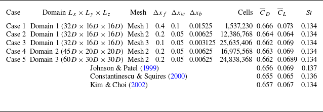
Before deciding the computational domain, we carried out domain-independent simulations, as detailed in table 2, following previous studies (e.g. Saha Reference Saha2004; Khan et al. Reference Khan, Khan, Sharma and Agrawal2020; Sarkar & De Reference Sarkar and De2025). Based on these simulations, we arrived at a cuboid domain with a streamwise length of
 $32D$
and a cross-sectional area of
 $16D\times 16D$
; here,
 $D$
denotes the characteristic length of the elliptical cap. In this domain, the blockage is found to be only
 $0.30\,\%$
. A schematic of the computational domain is shown in figure 4.
We used the snappyHexMesh function of OpenFOAM to generate a mesh with hexahedral elements. Key mesh quality parameters include an aspect ratio of
 $7.3629$
, max non-orthogonality
 $53.1225$
and average of
 $3.7581$
and max skewness
 $0.6966$
. We use a large number of elements near the body and in the wake to resolve wake features of the flow accurately, as illustrated in figure 4(b). The mesh resolution (spatial resolution) in various regions of the domain was set as follows: near the body,
 $\varDelta =0.0025$
, wake region,
 $\varDelta =0.05$
and far field,
 $\varDelta =0.2$
.
To simulate the flow over the elliptical cap model, we use ‘IcoFoam’, which is a transient solver for an incompressible flow of the open source platform, OpenFOAM. This transient solver in OpenFOAM is designed for an incompressible flow that employs the pressure-implicit with splitting of operators (PISO) algorithm. The governing (2.4) were discretised using the second-order Crank–Nicolson scheme for time and the Gauss linear quadrature scheme for space. The PISO algorithm adopts a predictor–corrector strategy to iteratively solve for the velocity and pressure fields, ensuring proper coupling between these two fields. We use an inflow boundary condition as
 $ u = U_{\infty }$
at the inlet, a no-slip boundary condition on the model surface and free-slip boundary conditions at the top, bottom and both sides of the domain. For the free-slip boundary conditions, the normal component of the velocity and the normal gradient of the tangential velocity component were made equal to zero. To maintain the numerical stability and the Courant–Friedrichs–Lewy (CFL) number less than 1, we used a time step size of
 $\Delta t=0.0025$
, resulting the mean CFL to be 0.01 and the maximum CFL to be 0.6. The convergence of the simulation was monitored based on the residuals, which were required to be below
 $10^{-6}$
for all variables.
2.5. Validation: flow over sphere
We have considered the flow past a sphere for validation of our numerical approach. The linear stability analysis for the flow over a sphere has been carried out to find the primary and secondary bifurcations, whereas the DNS for the sphere has been carried out at
 ${\textit{Re}} = 300$
to investigate the mesh and domain independence. For the linear stability analysis, we have first simulated the flow past a sphere at Reynolds number,
 ${\textit{Re}} = 50$
, to get an initial guess flow field for the base flow calculation at the same
 ${\textit{Re}}$
. Following this calculation, we have calculated the base flow using the Newton–Raphson method, and the linear stability analysis has been carried out to investigate the growth of the small perturbations about this calculated base flow.
To assess the domain and the mesh independence for the stability analysis, the critical Reynolds number was examined for two different domain sizes (domain 1 and domain 2) and for three different meshes (mesh 1, mesh 2 and mesh 3). The computational domain was enclosed within a cylindrical boundary of radius
 $r_{\infty } = 30D$
. For the initial simulation, the inlet and outlet boundaries were located at
 $x_{-\infty } = -30D$
and
 $x_{\infty } = 400D$
, respectively, where
 $D$
is the diameter of the sphere. In subsequent tests, the outlet was shifted to
 $x_{\infty } = 200D$
. As shown in table 1, domain 2 with
 $x_{\infty } = 200D$
and mesh 2 was found to be sufficient to reproduce the critical Reynolds numbers accurately for the primary and secondary bifurcations, as these values compare well with the data reported in the literature (Meliga et al. Reference Meliga, Chomaz and Sipp2009; Zheng, Pan & Ni Reference Zheng, Pan and Ni2023). Further, we calculated the coefficient of drag and the recirculation length from the base flow, which also compare well with the data of Pier (Reference Pier2008), as shown in figure 5.
Validation of flow over sphere by comparing
 ${\textit{Re}}$
for primary and secondary bifurcations with grid and domain independence by global linear stability analysis. The same mesh distribution is used for cases 1 and 2, with a varying streamwise domain length to check the influence of domain extent on the stability results.

Comparison with Pier (Reference Pier2008). (a) Coefficient of drag
 $C_d$
and (b) recirculation length
 $L_R$
of the base flows for various aspect ratios.

Similarly, we have carried out the domain and mesh independence study for the three-dimensional (3-D) DNS for the flow over a sphere at
 ${\textit{Re}}=300$
. The mean drag (
 $\overline {C}_{D}$
) and lift (
 $\overline {C}_{L}$
) coefficients and the Strouhal number (
 ${\textit{St}}$
) are calculated for different domains and meshes. One can notice that the data for case 2 compares well with the data reported in the literature (Johnson & Patel Reference Johnson and Patel1999; Constantinescu & Squires Reference Constantinescu and Squires2000; Kim & Choi Reference Kim and Choi2002), as seen in table 2.
Mesh and domain independence test cases for the flow over a sphere at
 ${\textit{Re}} =300$
. We have finally chosen case 2 for the DNS reported in this article. Here,
 $\Delta x_{{f}}$
,
 $\Delta x_{{w}}$
and
 $\Delta x_{{b}}$
denote the mesh spacing at the far field, wake and body, respectively.

2.6. Experimental methods and techniques
All the experiments reported here were performed in a water tunnel. It has a test section of
 $180$
in width,
 $250$
in depth and
 $460$
mm in length. The flow speed in the tunnel is controlled by a speed controller, and it can be varied from
 $10$
to
 $100$
mm s−1. This tunnel was used in various previous works (e.g. Bhattacharyya et al. Reference Bhattacharyya, Khan, Verma, Kumar and Poddar2022; Sunil, Kumar & Poddar Reference Sunil, Kumar and Poddar2022; Khan et al. Reference Khan, Sunil, Bhattacharyya, Yadav, Poddar and Kumar2023). Figure 6 shows a simple schematic of the present experimental arrangement in the test section of the water tunnel. The model placed in the middle of the test section using a support-sting (see figure 6) has a base diameter of 10 mm. The support-sting was made of a hollow tube of diameter
 $1.1$
mm to inject dye into the flow. We may mention that Gumowski et al. (Reference Gumowski, Miedzik, Goujon-Durand, Jenffer and Wesfreid2008) and Szaltys et al. (Reference Szaltys, Chrust, Przadka, Goujon-Durand, Tuckerman and Wesfreid2012) also used a similar dye injection system.
Schematic of the experimental set-up with right-handed Cartesian coordinate system (
 $x,y,z$
), where
 $x$
,
 $y$
and
 $z$
denote the streamwise, wall-normal and spanwise directions, respectively. (a) Water tunnel A: plenum, B: honeycomb and screen, C: contraction, D: test section, E: reticulation chamber (send water back to plenum) and F: transparent window. (b) Experimental set-up for simultaneous LIF visualisations. where the flow is from left to right, as shown by an arrow. (c) Schematic sketch for 2D-PIV in the
 $x{-}y$
plane. (a similar set-up was used for the other plane, as well).

In the present study, the laser-induced fluorescence (LIF) technique was used for flow visualisation (Sunil et al. Reference Sunil, Kumar and Poddar2022). We have used Rhodamine-B as the dye for flow visualisations. Since the dye injection tube (made of stainless steel) has a small diameter (
 ${\approx} 1.1\rm \,mm$
), it does not significantly affect the uniform flow in the test section. A continuous laser (5 W) is used to illuminate the dye. The flow rate of the dye solution is carefully controlled such that a minimum amount of dye is released in the flow to avoid its influence on the wake structure. The flow visualisation images were acquired using a DSLR camera (Nikon, model D850,
 $3820$
pixels
 $ \times 2460$
pixels) at 30 frames per second for a region of interest of 200 mm
 $\times$
100 mm. More than 9000 images were acquired for each experimental run, which were then analysed using the MATLAB image processing tool. Flow characteristics, such as the vortex shedding frequency, were calculated using the time series of these acquired images. We also carried out simultaneous dual-plane flow visualisations using two cameras in two different orthogonal planes for better characterisations of the wake.
The velocity fields in two different planes were obtained using the 2-D particle-image-velocimetry (2D-PIV) technique. The PIV measurements were performed in the wake region, downstream of the model, as shown in figure 6(c). The set-up for the same LIF technique was modified for the PIV measurements by replacing the continuous laser and the DSLR camera with a Nd:YAG double-pulsed laser (Quantel, EverGreen model with 200 mJ/pulse) and compatible CCD cameras (TSI, USA) with resolutions of 3312
 $\times$
2488 pixels (8 MP) at 1.45 Hz and 4912
 $\times$
3280 pixels (16 MP) at 1 Hz in double exposure mode, respectively. The experimental measurements were made using the first CCD camera (8 MP) unless otherwise stated explicitly. The flow was seeded with hollow glass spheres of approximate diameter 10
 $\rm \mu m$
. The required flow region was illuminated with
 ${\approx}$
1 mm thickness of laser sheet, and 1200 snapshots (600 pairs) were acquired for each case for an acquisition time of
 ${\approx}$
414 s. The acquired images were post-processed using ProVisionXS (IDTpiv), with a 32
 $\times$
32 pixels correlation window. The uncertainty in velocity was estimated to be approximately 3 % of the maximum streamwise velocity. This PIV system and the processing software were also used in our various previous studies (Balamurugan & Mandal Reference Balamurugan and Mandal2017; Sunil et al. Reference Sunil, Kumar and Poddar2022; Aniffa et al. Reference Aniffa, Caesar, Dabaria and Mandal2023).
2.7. Proper orthogonal decomposition analysis
Proper orthogonal decomposition (POD) helps identify coherent structures in unsteady flows and provides additional insights into the underlying flow dynamics. We briefly describe the technique, which is based on decomposing the fluctuating velocity field into spatial modes and their corresponding temporal coefficients.
Briefly, this technique provides basis functions
 $\boldsymbol{\varPhi }^{(k)}(\boldsymbol{x})$
that can represent a random function, such as a fluctuating velocity field
 $\boldsymbol{v}^\prime (\boldsymbol{x},t)$
, as (Berkooz, Holmes & Lumley Reference Berkooz, Holmes and Lumley1993)
 \begin{equation} \boldsymbol{v}^\prime (\boldsymbol{x},t) \approx \sum _{i=1}^k a^{(k)}(t)\,\boldsymbol{\varPhi }^{(k)}(\boldsymbol{x}), \end{equation}
where,
 $a$
,
 $\boldsymbol{\varPhi }$
and
 $k$
represent the time coefficient, the spatial POD mode shape and the mode index, respectively. It should be noted that the fluctuating velocity field,
 $\boldsymbol{v}^\prime (\boldsymbol{x},t)$
, comprises the fluctuating streamwise velocity,
 $u_x^{\prime}$
(
 $=$
instantaneous velocity,
 $u_x$
– mean velocity
 $\overline {u}_x$
) and the fluctuating transverse velocity,
 $u_y^{\prime}$
(
 $=$
instantaneous velocity,
 $u_y$
, – mean velocity,
 $\overline {u}_y)$
, in the present study. Here, the POD mode shapes are obtained using the method of snapshots (Sirovich Reference Sirovich1987). The fluctuating flow field
 $\boldsymbol{v}^\prime$
from each PIV snapshot is arranged into a matrix
 $A$
, and the covariance matrix
 $C$
is then obtained as
 $C = A^{T}A$
. The eigenvalues
 $\lambda _k$
of the matrix
 $C$
are then computed, which indicate the energy levels associated with each POD mode. The spatial POD modes are calculated as
 \begin{equation} \boldsymbol{\varPhi }_k = \sum _{i=1}^{M} \phi _{i}^k \boldsymbol{v}^\prime _{i}, \end{equation}
where
 $M$
is the number of snapshots and
 $\phi^{k}_{i}$
is the
 $i^{\mathrm{th}}$
component of the
 $k^{\mathrm{th}}$
eigenvector of the matrix
 $C$
. The time coefficients
 $(a_k)$
are then obtained using the inner product of
 $\boldsymbol{v}^\prime$
and
 $\boldsymbol{\varPhi }_k$
as
 $a_k = (\boldsymbol{v}', \boldsymbol{\varPhi }_k)$
. The relative energy,
 $E_r$
(in
 $\%$
), of the POD modes is calculated as
 \begin{equation} E_r = \frac {\lambda _r}{\sum _{i=1}^n \lambda _r} \times 100 \,\%. \end{equation}
The reader may refer to Mandal, Venkatakrishnan & Dey (Reference Mandal, Venkatakrishnan and Dey2010) and Dutta et al. (Reference Dutta, Kanshana, Gopalakrishnan and Mandal2022), for further details.
3. Base flow fields and global stability characteristics
The present section considers the base flow fields obtained for moderate Reynolds numbers at varying aspect ratios. We consider the elliptical cap bluff body to characterise the global flow behaviour at varying aspect ratios. The effect of the geometrical shape used to model the bluff body (elliptical/spherical) is discussed subsequently. The numerically obtained results are compared with the experimental observations in the next section.
3.1. Basic velocity fields
The steady axisymmetric base flow field for an elliptical cap at
 ${\textit{Re}}=100$
is illustrated in figure 7, where the streamlines are superimposed on contour of the azimuthal vorticity
 $\omega _{\theta } \equiv \partial _{x} u_{r} - \partial _{r}u_{x}$
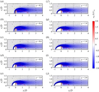
for varying aspect ratios. The flow separates at the downstream edge of the axisymmetric bluff body and rejoins in the wake to form a toroidal recirculating region. The shear layer developing on the surface of the elliptical cap rolls up at its base, which is the region where the vorticity fields have their maxima. This is evident at lower aspect ratios wherein the spatial gradients of vorticity are more pronounced in the lee side of the bluff body, as shown in figure 7. It can also be noted that the length of the recirculation bubble decreases with increasing aspect ratio, which is expected as the spatial extent of the favourable pressure gradient increases with
 $\chi$
. Similar observations have been made for flow past planar symmetric bluff bodies with increasing aspect ratio (Chiarini et al. Reference Chiarini, Quadrio and Auteri2022).
Base flow of elliptical shapes for different aspect ratios
 $\chi = 0.2$
to
 $2.0$
at
 ${\textit{Re}} = 100$
. Streamlines are plotted on top of a vorticity map
 $(\omega _\theta = \partial _x u_r - \partial _r u_x)$
, with the symmetric blue-to-red colour map in the range of
 $-2 \leqslant \omega _\theta \leqslant 2$
. The red solid line represents the recirculation zone.

The recirculation length is considered as the streamwise distance from the base of the model to the stagnation point in the wake along the centreline, and it is normalised by the base diameter
 $D$
. The dimensionless recirculation length
 $L_R$
for various Reynolds numbers is presented in figure 8(a). It can be seen that
 $L_R$
decreases with increasing aspect ratio for a fixed value of the Reynolds number. The spatial extent of the recirculation zone is of relevance as the nonlinear interactions between the modes take place within this absolutely unstable region, thereby effectively acting as a wave maker (Meliga et al. Reference Meliga, Chomaz and Sipp2009). The observed trend of
 $L_R$
with
 ${\textit{Re}}$
and
 $\chi$
can be summarised by re-scaling it using the Reynolds number as a parameter, which is shown in figure 8(b). We can see that the re-scaled value of
 $L_R$
is approximately a constant (
 $\sim$
0.3–0.4) for different values of
 $\chi$
, as compared with the unscaled variation (figure 8
b). The maximum reverse-flow velocity within the recirculating region
 $U_{\textit{rev}}$
(normalised by the free-stream velocity
 $U_\infty$
) is another quantity of interest to quantify the base flow characteristics. Its variation with aspect ratio for increasing values of
 ${\textit{Re}}$
is shown in figure 8(c). As observed for
 $L_R$
, the maximum reverse-flow velocity also decreases with increasing aspect ratio for a fixed value of the Reynolds number. The re-scaled values of
 $U_{\textit{rev}}$
, as shown in figure 8(d), collapse to a single curve for different Reynolds numbers and vary approximately from 0.03 to 0.05 for different values of
 $\chi$
. However, as the unscaled
 $L_R$
and
 $U_{\textit{rev}}$
decrease with increasing
 $\chi$
, we expect increasing aspect ratio to have a stabilising effect on the flow.
(a, c) Recirculation length
 $L_R$
and the maximum reverse-flow velocity
 $U_{\textit{rev}}$
within the recirculation zone as a function of the aspect ratio for increasing values of Reynolds numbers (denoted using an arrow). (b, d) Re-scaled values of
 $L_R$
and
 $U_{\textit{rev}}$
. Parameter settings:
 $100 \leqslant Re \leqslant 300$
.

3.2. Global stability analysis
The global linear stability analyses were carried out on the base flow fields described in the preceding subsection. Figure 9 shows the eigenvalue spectrum corresponding to the flow past a hemisphere with
 $\chi = 1$
for different values of the azimuthal mode number
 $m$
. As observed in earlier studies on bluff-body flows, the leading global mode corresponds to
 $m = 1$
with the primary bifurcation (shown in figure 9
a) being a stationary one with
 $\omega = 0$
at the critical Reynolds number
 ${\textit{Re}}_{c1} = 170.1$
. At a higher Reynolds number, the flow undergoes a Hopf bifurcation with a non-zero value for
 $\omega$
at
 ${\textit{Re}}_{c2} = 189.9$
(shown in figure 9
b). The Strouhal number corresponding to the secondary bifurcation is found to be
 $0.1267$
. These values are in excellent agreement with those reported in Jiménez-González et al. (Reference Jiménez-González, Manglano-Villamarín and Coenen2019) for the case of a hemisphere.
Eigenvalue spectrum for different azimuthal mode numbers
 $m$
corresponding to the (a) primary bifurcation at
 ${\textit{Re}}_{c1} = 170.1$
, and the (b) secondary bifurcation at
 ${\textit{Re}}_{c2} = 189.9$
. Parameter settings:
 $\chi = 1$
; hemisphere.

Figure 10 shows the variation of the temporal growth rate
 $\sigma$
corresponding to the leading global mode as a function of the Reynolds number at different aspect ratios. It can be seen that the critical Reynolds number increases with increasing aspect ratio for both the primary and secondary bifurcations, which are shown in figures 10(a) and 10(b), respectively. One can notice that
 $\sigma$
varies almost linearly with
 ${\textit{Re}}$
. It can be related using the Landau model (Landau Reference Landau1944) as
 \begin{equation} \sigma = C(\textit{Re} - \textit{Re}_{c}) \frac {\nu }{D^2}, \end{equation}
where
 $C$
is a constant, which can vary based on the shape of the bluff body and the nature of bifurcation, and
 $D$
is a typical length scale associated with the geometry. Earlier studies have reported
 $C = 0.2$
for flow past a cylinder, whereas
 $C = 0.6$
for the wake of a sphere (Provansal, Mathis & Boyer Reference Provansal, Mathis and Boyer1987; Sreenivasan, Strykowski & Olinger Reference Sreenivasan, Strykowski and Olinger1987; Ormières & Provansal Reference Ormières and Provansal1999; Thompson, Leweke & Provansal Reference Thompson, Leweke and Provansal2001; Schouveiler & Provansal Reference Schouveiler and Provansal2002; Provansal, Schouveiler & Leweke Reference Provansal, Schouveiler and Leweke2004). Furthermore, different values have been chosen in the literature for the flow past a sphere corresponding to the primary and secondary bifurcations. For instance, Ghidersa & Dušek (Reference Ghidersa and Dušek2000) and Thompson et al. (Reference Thompson, Leweke and Provansal2001) considered
 $C = 0.5$
for the secondary bifurcation, whereas Provansal et al. (Reference Provansal, Schouveiler and Leweke2004) considered
 $C=0.6$
for both primary and secondary bifurcations. In the present study, we have used a linear fit to determine the value of constant
 $C$
as a function of the aspect ratio
 $\chi$
, which is shown in figure 10 in panels (c) and (d) for the primary and secondary bifurcations, respectively. We can see that the value of
 $C$
decreases with
 $\chi$
and falls in the range of
 $0.4$
–
 $0.6$
.
Growth rate as a function of the Reynolds number for various aspect ratios of elliptical shape. (a) Primary (stationary) bifurcation and (b) secondary (oscillatory) bifurcation, with a modified constant value for the linear fit. (c–d) Values of the constant C (defined in (3.1)) for different aspect ratios for primary bifurcation and for secondary bifurcation.

The spatial distribution of the eigenmodes at
 ${\textit{Re}}_{c1}$
and
 ${\textit{Re}}_{c2}$
for
 $\chi = 1$
are shown in figures 11 and 12, respectively. The structure of
 $\hat {u}_{x}$
,
 $\hat {u}_{r}$
and
 $\hat {u}_{\theta }$
corresponding to the primary bifurcation shows that the leading global mode is dominated by axially extending streamwise disturbances. As the leading global mode corresponds to the azimuthal mode number
 $m = 1$
, the axial velocity perturbation is opposite on the other side of the axis of revolution. The radial and azimuthal velocity perturbations are primarily dominant in the near-wake region. These spatial distributions are typical of stationary bifurcations observed in axisymmetric flows past bluff bodies, which we have also observed using dual-plane experimental flow visualisations (discussed in the subsequent section). On the other hand, the leading global mode at
 ${\textit{Re}}_{c2}$
has spatially periodic variations along the axial direction, which is characteristic of an oscillatory bifurcation, as shown in figure 12. Similar spatial distributions are also observed for other aspect ratios.
Spatial distribution of the leading global mode at the primary stationary bifurcation. The real part of the velocity perturbations normalised by their maxima: (a)
 $\hat {u}_x$
, (b)
 $\hat {u}_r$
and (c)
 $\hat {u}_{\theta }$
. Parameter settings :
 ${\textit{Re}} = 170.1$
,
 $\chi = 1$
,
 $m = 1$
.

Spatial distribution of the leading global mode at the secondary oscillatory bifurcation. The real part of the velocity perturbations normalised by their maxima: (a)
 $\hat {u}_x$
, (b)
 $\hat {u}_r$
and (c)
 $\hat {u}_{\theta }$
. Parameter settings :
 ${\textit{Re}} = 189.9$
,
 $\chi = 1$
,
 $m = 1$
.

(a) Critical Reynolds numbers corresponding to the primary (
 ${\textit{Re}}_{c1}$
) and secondary (
 ${\textit{Re}}_{c2}$
) bifurcations as a function of the aspect ratio
 $\chi$
. (b) Critical Reynolds numbers rescaled using the recirculation length
 $L_R$
and the maximum reverse-flow velocity
 $U_{\textit{rev}}$
such that
 ${\textit{Re}}^{*}=U_{\textit{rev}}L_R /\nu$
as a function of the aspect ratio. It can be seen that the rescaled critical Reynolds number corresponding to the primary bifurcation remains approximately a constant at different values of
 $\chi$
.

Figure 13(a) shows the variation of the critical Reynolds number corresponding to the primary (
 ${\textit{Re}}_{c1}$
) and secondary (
 ${\textit{Re}}_{c2}$
) bifurcations as a function of the aspect ratio. The aspect ratio
 $\chi$
has been varied from 0.2 to 2.0 in the present study. The values of
 ${\textit{Re}}_{c1}$
and
 ${\textit{Re}}_{c2}$
at
 $\chi = 2$
are
 $216.3$
and
 $261.4$
, respectively, which are in excellent agreement with Bohorquez et al. (Reference Bohorquez, Sanmiguel-Rojas, Sevilla, Jiménez-González and Martínez-Bazán2011) (
 $L/D = 1$
in their study). Similarly, the values of
 ${\textit{Re}}_{c1}$
and
 ${\textit{Re}}_{c2}$
at
 $\chi = 0.2$
are found to be 127.9 and 136.7, which are comparable to the corresponding values of 116.9 and 125.3 as reported by Meliga et al. (Reference Meliga, Chomaz and Sipp2009) for a disk. It should be noted that the shape of the present model at
 $\chi = 0.2$
is similar to a disk, but not a complete disk. Further, we find the primary bifurcation at
 ${\textit{Re}} = 170.1$
for the model with
 $\chi = 1.0$
(a hemisphere), which is in good agreement with the findings of Jiménez-González et al. (Reference Jiménez-González, Manglano-Villamarín and Coenen2019), who also used a steady axisymmetric base flow for linear stability analysis. Kim & Choi (Reference Kim and Choi2003) reported the onset of primary bifurcation in the range of
 $180 \lt Re \lt 190$
and the secondary bifurcation in the range of
 $200 \lt Re \lt 210$
for hemispherical geometries. These observations are found to be consistent with the present trends.
We can see that increasing the aspect ratio has a stabilising effect as mentioned earlier. This is consistent with the fact that
 $L_R$
, which characterises the spatial extent of the absolutely unstable region, and
 $U_{\textit{rev}}$
, which is a measure of the growth of disturbances which travel upstream, both decrease with increasing
 $\chi$
. Furthermore, the boundary layer thickness at the point of separation increases with an increase in the length of the bluff body, leading to a thickening of the shear layer resulting in an increased diffusion of the shear layer and a weaker instability. Using
 $L_R$
and
 $U_{\textit{rev}}$
as the length and velocity scales, we have rescaled the critical Reynolds number, which is shown in figure 13(b) as a function of the aspect ratio. Interestingly, the rescaled critical value of the Reynolds number corresponding to the primary bifurcation is approximately a constant for different values of
 $\chi$
. The critical Reynolds number corresponding to the secondary bifurcation shows a larger variation within the investigated range of aspect ratios. This may be due to the consideration of axisymmetric base flow even after primary bifurcation, which is actually not axisymmetric beyond the primary bifurcation (e.g. Pier Reference Pier2008). However, this aspect needs to be investigated further. Considering the scaled
 ${\textit{Re}}_{*}$
as shown in figure 13(b), one can rewrite the (3.1) as
 \begin{equation} \sigma = C^*({\textit{Re}}^* - {\textit{Re}}^*_{c}) \frac {\nu }{L^2_{\mathrm{R}}}, \end{equation}
where
 $C^*$
is a constant, and
 ${\textit{Re}}^* = U_{\textit{rev}} L_{\mathrm{R}} /\nu$
. The Landau constant,
 $C^*$
, is found to be approximately
 $1$
for both the primary and secondary bifurcations.
To summarise, we have presented the base flow fields and the stability characteristics corresponding to the bubble-shaped geometries modelled as an elliptical cap in this section. We now proceed to compare the obtained results with experimental measurements and visualisations in the following section.
4. Comparison with DNS and experimental observations
For experimental characterisations, we have carried out simultaneous dye flow visualisations in two different orthogonal planes. For quantitative flow visualisations, we have also carried out the PIV measurements. Figures 14(a) and 14(b) show the simultaneous flow visualisations in the
 $x$
–
 $z$
and
 $x$
–
 $y$
planes, respectively. These visualisations are obtained using the LIF technique at
 ${\textit{Re}} = 150$
, which is slightly above the critical value
 ${\textit{Re}}_{c1} = 149.2$
corresponding to the primary bifurcation. The bubble shape is modelled as an elliptical cap of aspect ratio
 $\chi = 0.6$
. The wake is characterised by two trailing counter-rotating vortices with the injected dye being trapped in the vortex cores. This observation is further supported by the DNS data, as shown in figures 14(c) and 14(d) in terms of the iso-surface of streamwise vorticity,
 $\omega _x = ({\partial w}/{\partial y} - {\partial v}/{\partial z}$
). However, this results in a two-threaded structure which is clearly visible in the top view (
 $x$
–
 $z$
plane) shown in figure 14(a). The observed mode manifests itself through a tilting of the recirculating region in the near wake of the bluff body, and is attributed to the breaking of axisymmetry rather than to the splitting of a thread into two. The counter-rotating vortices in the wake induce a velocity along the centreline resulting in a convective displacement of the two threads with respect to each other. This results in an increase in the gap between the threads along the axial direction which can also be seen in the top view. The stationary nature of the bifurcation is also clearly captured, as no oscillation is observed for the dye streaks. Furthermore, the flow visualisations clearly indicate that the axisymmetry is replaced by a planar symmetry.
(a–b) The LIF visualisations of flow (from left to right) past an elliptical cap of aspect ratio
 $\chi = 0.6$
at
 ${\textit{Re}} \approx 150$
. The Reynolds number is slightly above the critical value corresponding to the primary bifurcation. The stationary double-threaded bifid structure of the wake is clearly visible with a planar symmetry. (a) Top view in the
 $x$
–
 $z$
plane, and (b) side view in the
 $x$
–
 $y$
plane. (c–d) Iso-surfaces of vorticity,
 $\omega _x = {\partial w}/{\partial y} - {\partial v}/{\partial z}$
obtained from DNS data for the elliptical cap at
 $\chi = 0.6$
and
 ${\textit{Re}}= 153$
. (c) Top view in the
 $x$
–
 $z$
plane, and (d) side view in the
 $x$
–
 $y$
plane.

(a–b) The LIF visualisation corresponding to the secondary oscillatory bifurcation for
 $\chi = 0.6$
at
 ${\textit{Re}} \approx 162$
. The trailing counter-rotating vortices get connected to each other resulting in the formation of skewed loops.(a) Top view in the
 $x{-}z$
plane. (b) Side view in the
 $x{-}y$
plane. The dash line shows the recirculation region and
 $L_R \approx 1.8$
whereas the base flow,
 $L_R = 1.98$
. (c–d) Iso-surfaces of
 $\lambda _2$
criterion obtained from the DNS data for the elliptical cap model with
 $\chi = 0.6$
at
 ${\textit{Re}} = 167$
. (c) Top view
 $x{-}z$
plane. (d) Side view
 $x{-}y$
plane.

As the Reynolds number is increased further, the flow undergoes an oscillatory bifurcation at
 ${\textit{Re}}_{c2} = 162$
for
 $\chi = 0.6$
. This is shown in figures 15(a) and 15(b) wherein the trailing counter-rotating vortices get connected to each other, resulting in the formation of strongly skewed loops which get convected downstream. We may note that these visualisations in two different planes were also performed simultaneously using two cameras. However, the flow retains the plane of symmetry selected at the previous bifurcation, as seen in the flow visualisations in the cross-flow plane. One may notice in figure 15(b) that there exists a lateral displacement of the shed vortices while moving downstream. This is due to the fact that the velocity of the counter-rotating vortices in the wake is always directed in one way (see Gumowski et al. Reference Gumowski, Miedzik, Goujon-Durand, Jenffer and Wesfreid2008), resulting a lateral movement. The DNS data, as shown in figures 15(c) and 15(d), in terms of the iso-surfaces of
 $\lambda _2$
(Jeong & Hussain Reference Jeong and Hussain1995), also show similar results visualised using the LIF technique.
Figure 16(a) schematically shows the cross-flow plane for the LIF visualisation. We have carried out cross-flow visualisations for two different models with aspect ratios,
 $\chi = 0.6$
and
 $\chi = 2.0$
. Figures 16(b) and 16(c) show the LIF visualisations at different instants of time within a period of oscillation, for aspect ratios
 $\chi = 0.6$
at
 ${\textit{Re}} \approx 162$
and
 $\chi = 2.0$
at
 ${\textit{Re}} \approx 249$
, respectively. It should be noted that a laser sheet from the continuous laser was used in the cross-flow plane for this visualisation (figure 16
a). However, one can clearly notice that there exists a plane of symmetry in these visualisations. Although the same holding device was used to hold both the models, the plane of symmetry changes due to the change of the aspect ratio, as seen in figures 16(b) and 16(c). It was also found that the plane of symmetry for a particular model does not change its orientation with an increase in Reynolds number beyond the secondary bifurcation. However, it must be noted that, although the angular orientation of this plane in principle is selected by the vertical orientation of the support system in experiments, the perturbations induced by the holding device may indeed modify it, resulting in the selection of a different symmetry plane. These observations are in excellent agreement with those made for flows past other axisymmetric bluff bodies where the vortex shedding regimes are characterised by the rotation of a symmetry plane (Fabre et al. Reference Fabre, Auguste and Magnaudet2008) leading to a ‘kinking’ of vortex threads (Shenoy & Kleinstreuer Reference Shenoy and Kleinstreuer2008), resulting in a shifted hairpin shedding (Meliga et al. Reference Meliga, Chomaz and Sipp2009; Bobinski et al. Reference Bobinski, Goujon-Durand and Wesfreid2014).
(a) Schematic for the visualisations in the cross-flow plane. Cross-flow visualisations using the LIF technique corresponding to the secondary oscillatory bifurcation for aspect ratios
 $\chi = 0.6$
at
 ${\textit{Re}} \approx 162$
(b) and
 $\chi = 2.0$
at
 ${\textit{Re}} \approx 249$
(c). The trailing counter-rotating vortices get connected to each other resulting in the formation of skewed loops. Here,
 $T$
denotes the time period of one oscillation. The dashed line in (b) at 0.375T instant indicates the plane of symmetry.

Similar flow features were observed at other aspect ratios. The flow fields at different time instants obtained using the LIF technique for
 $\chi = 2$
at the Reynolds number corresponding to the secondary bifurcation are shown in figure 17. The observed wake structure reveals that the flow fields indeed do exhibit a planar symmetry. Furthermore, it can be noticed that the extent of the recirculating region is considerably smaller in comparison with the flow fields observed at
 $\chi = 0.6$
(shown in figure 15
b). The critical Reynolds numbers,
 ${\textit{Re}}_{c1}$
and
 ${\textit{Re}}_{c2}$
, corresponding to the primary and secondary bifurcations observed experimentally, agree well with the predictions made using the global linear stability analyses of the axisymmetric base flow fields within the range of aspect ratios considered in the present study.
Sequences of LIF visualisations following the secondary oscillatory bifurcation for
 $\chi = 2$
at
 ${\textit{Re}} \approx 256$
. The bubble-shaped bluff body is modelled as an elliptical cap. As observed, the trailing-edge vortices form well-connected loops, retaining a plane of symmetry. The recirculation length is marked in dashed lines
 $L_R \approx 1.14, 1.41, 1.16$
for the figures from top to bottom. The base flow recirculation length for the same
 ${\textit{Re}}$
is
 $L_R = 1.79$
.

To further quantify and compare the experimental observations with the linear stability analyses, we have measured the vortex shedding frequency and the wavelength of the wake structure, as shown in figure 18. The time-series data of the intensity of the images are obtained at different spatial locations, as shown in figure 18(a). These locations are carefully chosen such that they are slightly offset from the axis, which ensures that a continuous stream of images with finite intensities is obtained. The data are collected over an interval of
 $2$
min, which corresponds to approximately 3600 images. The shedding frequency is then obtained by performing a Fourier transform, as shown in figure 18(b), where the fundamental frequency and higher harmonics are clearly captured. Although the measurements made closer to the bluff body have a higher amplitude, the global shedding frequency is indeed the same throughout the entire wake structure. The wavelength is obtained by calculating the average distance between the observed crests and troughs in the spatially well-developed region further downstream of the bluff body. The variations of the Strouhal number and the wavenumber as a function of the aspect ratio are shown in figures 19(a) and 19(b), respectively. The values from experimental measurements, made at three different aspect ratios, are shown alongside the numerically obtained values from the global stability analysis and these are in good agreement. It is interesting to observe that, although the recirculation lengths
 $L_R$
and the maximum reversed flow
 $U_{\textit{rev}}$
decrease with increasing aspect ratio, the dominant shedding frequency and the wavelength of the fundamental global mode remain constant throughout the entire range of
 $\chi = 0.2{-}2.0$
.
(a) The LIF visualisation illustrating the selected locations
 $(f_{L1}, f_{L2}, f_{L3}, f_{L4}, f_{L5})$
where image intensity (as a time-series data) were extracted from each frame. The peak-to-peak positions, marked as
 $\lambda$
to indicate one wavelength. (b) Variation of Strouhal number (
 ${\textit{St}} = fD/U$
) at the selected locations for the elliptical cap model with
 $\chi = 2.0$
at
 ${\textit{Re}} \approx 267$
; here
 $f$
in the Strouhal number expression is the shedding frequency in Hz.

(a) Frequency (
 ${\textit{St}} = \textit{f}D/U$
, Strouhal number) and (b) Wavenumber (
 $k=2\pi /\lambda$
) of the leading growth rate for secondary (oscillatory) bifurcation
 ${\textit{Re}}$
for different aspect ratios of elliptical model. Experimental details are discussed below.

We have carried out the PIV measurements to provide further insight into the flow fields. It should be noted that the PIV acquisition rate is more than four times the dominant shedding frequency. Figure 20 shows the time sequence of the streamwise vorticity (
 $\omega _z = \partial _{x} u_{y} - \partial _{y}u_{x}$
) in the
 $x$
–
 $z$
and
 $x$
–
 $y$
planes, which correspond to the top and side views, for
 $\chi = 0.6$
. The spatial distributions corresponding to the primary stationary bifurcation are shown in figures 20(a) and 20(b), for the top and side views, respectively, and those corresponding to the secondary oscillatory bifurcation in figures 20(c) and 20(d), respectively. The time sequence of both views clearly shows that the wake is steady after the primary bifurcation, whereas the same is unsteady or oscillatory in nature after the secondary bifurcation. Further, considering the slope in terms of diverging angle of the two threads in figures 14(a,c) and 20(a), we find these values to be approximately
 $3.1$
,
 $2.3$
and
 $2.4$
degrees based on the LIF, PIV and DNS data, respectively. Therefore, the flow features that were observed using the LIF technique are correctly captured using the PIV measurements. Although the flow fields are non-axisymmetric, one can clearly deduce the existence of a plane of symmetry (on average over a shedding period) in the wake after the primary and secondary bifurcations, which is consistent with the theoretical predictions reported in the literature (Ghidersa & Dušek Reference Ghidersa and Dušek2000; Fabre et al. Reference Fabre, Auguste and Magnaudet2008; Meliga et al. Reference Meliga, Chomaz and Sipp2009).
Time sequences of the streamwise vorticity for the primary
 $(Re \approx 150)$
(a–b) and secondary
 $(Re \approx 162)$
(c–d) bifurcations obtained from PIV measurements of the elliptical cap (
 $\chi = 0.6.$
). The flow direction is from left to right. The contour represents the downstream flow field relative to the model, with the origin located at the centre of the base of the model. The arrows indicate the fluctuating velocity vectors, composed of the fluctuating streamwise velocity,
 $u_x^{\prime}$
(
 $=u_x$
−
 $\overline {u}_x$
) and the fluctuating transverse velocity,
 $u_y^{\prime}$
(
 $=u_y$
−
 $\overline {u}_y$
). These vectors are in relative scale.

To further our understanding of the wake flow characteristics beyond the secondary bifurcation, we have carried out the POD analysis of the cross-stream fluctuating velocity
 $(u'_y)$
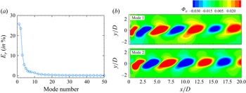
field obtained from the PIV measurements. Figure 21(a) shows the relative energy distribution of the different modes corresponding to
 $\chi = 0.6$
at
 ${\textit{Re}} \approx 178$
. The first two modes are the dominant ones, with the first 10 modes contributing to more than
 $80\,\%$
of the total energy. The spatial distributions of the first two modes are shown in figure 21(b). The contour plots clearly reveal the existence of a slight spatial shift between mode 1 and mode 2. Such a spatial shift associated with a pair of near degenerate POD modes is generally observed in the case of bluff-body wakes, and it is often attributed to the existence of the space–time symmetry in the flow (Noack & Eckelmann Reference Noack and Eckelmann1994; Dutta et al. Reference Dutta, Kanshana, Gopalakrishnan and Mandal2022). In the present case, the space–time symmetry comes from the periodic vortex shedding behind the model. Figures 15, 17 and 20(c–d) clearly show the vortex shedding that can be considered as a travelling wave/structure.
The POD analysis of the cross-stream fluctuating velocity
 $(u'_y)$
of elliptical shaped model
 $\chi = 0.6$
at
 ${\textit{Re}} \approx 178$
. (a) Relative energy (in %) vs POD mode; (b) POD mode 1 and mode 2.

Figure 22 shows comparisons of the base flow field with the mean velocity field, and the global mode shape with the POD mode shape obtained from the PIV and DNS data for
 $\chi = 0.6$
. The comparison of the data has been shown only in the
 $x$
–
 $y$
plane, as the dominant POD modes were obtained based on the PIV and DNS data in this plane. Figure 22(a–c) shows the base flow components and the leading global mode. The streamwise velocity component
 $(\bar {u}_x)$
and the radial velocity component
 $(\bar {u}_r)$
show a recirculation region near the separation point. The spatial structure of the global mode shows the coherent nature of the flow. The mean flow field and the leading POD mode, obtained from the PIV and DNS data, are shown in figures 22(d–f) and 22(g–i), respectively. One can see a similarity between the base flow and mean flow fields obtained from the experiments and numerical simulation. The mean flow contours, mainly
 $(\bar {u}_y)$
, show slight deviations from the corresponding base flow and DNS data. This may be due to the effect of the model holding device during the PIV acquisition. However, for better comparison, we have extracted the streamwise velocity (
 $\bar {u}_x$
) and the cross-stream velocity (
 $\bar {u}_y$
) components along the centreline of the wake from the PIV and DNS data and plotted in figures 23(a) and 23(b), respectively. The measured streamwise component quantitively compares well with the DNS data except in the region immediately downstream of the model, which is due to laser reflection from the model and a smaller number of identifiable tracer particles; whereas the cross-stream component shows a systematic deviation. This may be attributed to the fact that the cross-stream component is very small (
 ${\approx}$
4 % of
 $U_{\infty }$
or
 ${\approx}$
0.6 mm s−1), as compared with the streamwise component, and therefore, its measurement is also very difficult and prone to be noisy even with a 16 MP CCD camera in a larger field of view, as done here for the data shown in figure 22(d,e). The cross-stream velocity (
 $\bar {u}_y$
) component measured either with an 8 MP/16 MP CCD camera qualitatively follows a similar trend as in the base flow and DNS data. The global and the POD mode shapes, as can be seen in the last row of this figure, also compare well, at least qualitatively. This similarity is expected as the experimental and the DNS flow fields are close to the secondary bifurcation; to be explicit, the PIV and the DNS data are obtained at
 ${\textit{Re}}=178$
, whereas the global analysis leading to secondary bifurcation has been carried out at
 ${\textit{Re}}=162$
. Overall, the agreement between the global mode based on an axisymmetric base flow and the dominant POD mode extracted from both 2-D PIV and 3-D DNS data in the
 $x$
–
 $y$
plane confirms that the linear instability analysis can describe the underlying flow physics at secondary bifurcation.
Comparison of global linear stability analysis with POD of experimental and DNS results for
 $\chi =0.6$
. (a) Axial velocity (
 $\bar {u}_x$
) of base flow. (b) Radial velocity (
 $\bar {u}_r$
) of base flow. (c) The real part of
 $\hat {u}_r$
leading global mode at
 ${\textit{Re}} = 162$
for azimuthal wavenumber
 $m=1$
. (d) Mean velocity along the x-axis (
 $\overline{u}_{x}$
) and (e) mean velocity along the y-axis (
 $\overline{u}_{y}$
) of 600 snapshots. (f) First POD mode of
 $u'_y$
fluctuating velocity for
 ${\textit{Re}} \approx 178$
. (g) Mean flow velocity
 $\overline {u}_x$
along the x-axis from DNS. (h) Mean flow velocity
 $\overline {u}_x$
in the y-axis. (i) First POD mode of
 $u'_y$
fluctuating velocity of DNS for
 ${\textit{Re}} = 178$
.

Comparison of mean velocity field obtained from the PIV and DNS data along the centreline, with the base flow field. (a) The streamwise velocity component (
 $\overline {u}_x$
). (b) The cross-stream velocity component (
 $\overline {u}_y$
).

4.1. Effect of geometry
The effect of modelling the bubble-shaped geometries as elliptical and spherical caps is briefly investigated in this section. As discussed in § 2, these configurations are characterised by a circular base and the height of the bubble, with the bluff bodies modelled as spherical caps being a part of a sphere within the range
 $0.2 \leqslant \chi \leqslant 1$
(see figure 2). The base flow features from numerical simulations, such as the recirculation length
 $L_R$
and the maximum reverse-flow velocity
 $U_{\textit{rev}}$
, follow similar trends, with the same scaling laws, as observed in the case of elliptical caps (see figure 8). However, subtle differences were observed in the global stability characteristics, which are summarised in figure 24. The spherical cap model exhibits the onset of instability earlier than the elliptical cap model, indicating that the flow behind the elliptical cap is comparatively stable. Notably, both models have the same projected area (normal to the streamwise direction). However, the elliptical model has a curvature that gradually aligns with the streamwise direction, whereas the spherical model has a curvature that does not align as smoothly as the elliptical one. This difference in the edge geometry influences the flow characteristics, as further discussed below by examining the velocity and vorticity distributions near the sharp edge. The critical Reynolds numbers corresponding to spherical caps were found to be lower than the values of elliptical caps, with the differences being larger at lower aspect ratios. Although both models have the same sharp blunt edge at the base (see figure 2
c, red line curve and blue dashed-line curves), which initiates flow separation, the separation is more pronounced in the spherical cap model as compared with the elliptical cap model due to the sharper curvature. However, the rescaled values of the critical Reynolds numbers, using
 $L_R$
and
 $U_{\textit{rev}}$
, follow the same scaling law for both the configurations, as shown in figure 24(b). Furthermore, the differences in Strouhal numbers and the dominant wavenumbers, corresponding to the secondary bifurcation obtained from the global linear stability analysis, are found to be negligible, as shown in figure 25. Additionally, experiments were also carried out at
 $\chi =0.6$
for a spherical cap. We found similar flow features (not shown here for brevity) as in the case of an elliptical cap (figure 15). The Strouhal numbers corresponding to spherical and elliptical caps for
 $\chi = 0.6$
were
 $0.13$
, and
 $0.12$
, respectively. The Strouhal numbers calculated from experimental observations are
 $0.14 \pm 0.02$
for the spherical cap model and
 $0.12 \pm 0.02$
for the elliptical cap model. These values are comparatively higher than the Strouhal number predicted by the global linear stability analysis. The discrepancy may be attributed to uncertainties inherent in experimental measurements. Nevertheless, the observed Strouhal numbers fall within the limit of experimental uncertainty and are therefore considered to be in reasonable agreement with the numerical predictions. The spherical cap exhibits a sharper curvature at the separation point, which induces a larger separated wake and a stronger recirculation zone compared with the elliptical cap. This induces earlier vortex shedding and supports higher-frequency wake instabilities. Whereas the elliptical cap has a gradual curvature and a surface more aligned with the streamwise flow, which leads to smoother separation and consequently lower instability frequencies. Furthermore, the spherical cap generates stronger shear layers at the separation edge, which enhances the onset and growth rate of secondary instabilities, as discussed below.
Comparison of critical Reynolds number obtained from the linear stability analysis for the primary (stationary) and secondary (oscillatory) bifurcations of spherical and elliptical cap models with aspect ratios
 $\chi = 0.2{-}0.4$
. Panels show (a)
 ${\textit{Re}}$
 $ ( = {\rho UD}/{\mu } )$
versus
 $\chi$
and (b) scaled
 ${\textit{Re}}^*$
 $( = {\rho |u_{\textit{rev}}| L_R}/{\mu })$
versus
 $\chi$
.

(a) Frequency (
 ${\textit{St}}$
) and (b) wavenumber (
 $k$
) of the leading growth rate for secondary(oscillatory) bifurcation
 ${\textit{Re}}$
for different aspect ratios
 $\chi = 0.2{-}0.8$
of elliptical cap and spherical cap.

(a) Comparison of the streamwise velocity component of the base flow for the elliptical (solid line in red) and spherical cap (solid line in blue) models for
 $\chi =0.4$
and
 $\chi = 0.8$
at different Reynolds numbers. (b) Comparison of the transverse velocity component of the base flow for elliptical (solid line in red) and spherical cap (solid line in blue) models for
 $\chi =0.4$
and
 $\chi = 0.8$
at different Reynolds numbers. (c) Vorticity (
 $\omega _{\theta } = \partial _x \overline {u}_r - \partial _r \overline {u}_x$
) contours (
 $-20 \leqslant \omega _\theta \leqslant 20$
) at
 $\chi = 0.4$
for
 ${\textit{Re}} = 130$
for elliptical and spherical cap models, and at
 $\chi = 0.8$
for
 ${\textit{Re}} = 150$
.

In order to understand the origin of observed differences in the critical Reynolds numbers, especially at lower aspect ratios, we take a closer look at the base flow fields at the downstream edge of the bluff body, prior to flow separation. The variation of the streamwise (axial),
 $\overline {u}_x$
, and the transverse (radial),
 $\overline {u}_r$
, components of the base velocity field, along with the vorticity (
 $\omega _{\theta } = \partial _x \overline {u}_r - \partial _r \overline {u}_x$
) contours at
 $\chi$
= 0.4 and 0.8 are shown in figure 26 for different Reynolds numbers. We have considered Reynolds numbers that span the primary and secondary bifurcations. One can clearly see the differences in the profiles, which are more pronounced at
 $\chi = 0.4$
, for the streamwise and the transverse velocity components in figures 26(a) and 26(b), respectively. Specifically, the maximum value of
 $\overline {u}_x$
is larger in the boundary layer region at the downstream edge (
 $0 \leqslant r/D \leqslant 0.5$
) for the case of elliptical cap. On the other hand, the radial velocity component,
 $\overline {u}_r$
, is found to be larger for the case of spherical cap. This difference may be attributed to the variation in the surface curvature between the two geometries. The curved surface of the elliptical cap is more aligned with the streamwise direction, resulting in a smoother axial velocity distribution. In contrast, the spherical cap induces stronger radial effects due to its steeper curvature. This behaviour is further examined by analysing the vorticity, which incorporates both axial and radial velocity gradients. The vorticity contours with iso-lines ranging from –20 to 0, as shown in figure 26(c), exhibit stronger and more localised vorticity near the separation region; this can be deduced from the tighter spacing of the iso-lines. In contrast, the elliptical cap shows a broader distribution of vorticity, indicating a more diffused shear layer (e.g. the iso-line,
 $\omega _\theta = -20$
, is more distributed downstream in the elliptical case). Since the transverse velocity is stronger and the streamwise velocity is weaker, it is highly plausible that the stronger shear layer for the spherical cap model is more prone to being affected by the transverse velocity, leading to an earlier roll-up of the shear layer and a lower critical Reynolds number. This explains why the wakes of spherical caps become unstable at an earlier Reynolds number than elliptical caps.
5. Concluding remarks
The stability and dynamics of flows past axisymmetric bluff bodies, motivated by the shapes of bubbles rising in quiescent fluids, have been investigated both numerically and experimentally. The bubble-shaped bluff bodies were modelled as spherical and as elliptical caps, with a circular base of diameter
 $D$
, and by the height (or width) of the bubble
 $W$
. The geometries are characterised by the aspect ratio
 $\chi = W/(D/2)$
, which is varied within the range
 $0.2 \leqslant \chi \leqslant 1$
for the spherical cap, and
 $0.2 \leqslant \chi \leqslant 2$
for the elliptical cap. The recirculation length
 $L_R$
, which is one of the measures of the spatial extent of the absolutely unstable region, and the maximum reverse-flow velocity
 $U_{\textit{rev}}$
, which is a measure of the growth of disturbances that travel upstream, in the wake of the bluff bodies were found to decrease with increasing aspect ratio. Global linear stability analyses were carried out on axisymmetric base flow fields subject to 3-D perturbations. As observed in earlier studies on bluff-body wakes, the primary bifurcation is stationary, followed by an oscillatory secondary bifurcation, with the leading global mode corresponding to azimuthal wavenumber
 $m = 1$
. The critical Reynolds numbers were found to increase linearly with increasing aspect ratio. Furthermore, the critical Reynolds number corresponding to primary bifurcation is found to be independent of the aspect ratio when re-scaled using
 $L_R$
and
 $U_{\textit{rev}}$
as the length and velocity scales, respectively.
The wake flow characteristics were examined experimentally using the LIF and the PIV techniques. The LIF visualisations have shown that at the primary bifurcation the wake is characterised by two trailing counter-rotating vortices resulting in a stationary two-threaded bifid structure. As the Reynolds number is increased further, the vortices get connected to each other, resulting in the formation of strongly skewed loops which get convected downstream. These observations have also been confirmed using the 3-D DNS. Interestingly, cross-flow visualisations have revealed that the flow has a planar symmetry following the primary bifurcation, which is retained beyond the secondary bifurcation. The measured wavelengths and frequencies, and the critical Reynolds numbers obtained from experimental and DNS data are in good agreement with the values obtained using linear stability analyses performed on axisymmetric base flow fields. Furthermore, the POD analysis of the fluctuating cross-stream velocity obtained from the PIV and DNS data is found to be consistent with the global mode shape. The insights gained from the present study can be used for designing efficient control strategies of bluff-body wakes.
Acknowledgements
We gratefully acknowledge the use of the PARAM Sanganak high-performance computing facility. We extend our sincere thanks to Professor K. Poddar and the National Wind Tunnel Facility (NWTF) for providing the laser and camera used in the PIV experiments. We also thank Mr Vivek M., Mr H. Om, Mr Dorilal and Mr A. Yadav for their help with the experimental set-up.
Funding
The authors thank the partial financial support from the Aeronautics Research & Development Board (Grant Numbers ARDB/01/1031875/M/I and ARDB/01/1031880/M/I) and Indian Institute of Technology Kanpur (Grant Number IITK/ME/2022358).
Declaration of interests
The authors report no conflict of interest.