





Introduction
In modern wireless communication systems, low-pass filters (LPFs) with features such as sharp roll-off (RO), low insertion loss, high return loss, wide stopband, and high rejection levels are essential for selecting desired signals and suppressing harmonic and spurious interferences [Reference Hong and Lancaster1]. Among various implementations, microstrip-based LPFs have gained widespread adoption due to their compact size, low cost, ease of fabrication, and excellent compatibility with planar integration technology. These advantages make them particularly well-suited for high-frequency and compact system applications. However, conventional microstrip LPF designs are often constrained by relatively slow cutoff transitions and limited stopband bandwidth, which restrict their performance in scenarios demanding high selectivity and wide out-of-band suppression [Reference Pozar2].
To address this problem, several LPFs with sharp RO and wide stopband have been reported. For instance, in [Reference Hayati, Akbari and Salahi4], a split-ring resonator loaded with folded polygonal patches is employed to design an LPF with a wide stopband and very sharp RO. A compact LPF utilizing multiple transmission zeros for stopband extension is reported in [Reference Chen, Run-Shuo and Chu5]. The LPF in [Reference Kumar and Parihar6] employs three coupled stepped-impedance resonators, achieving a ROR of 440 dB/GHz and a spurious-free bandwidth up to 16 GHz with 15 dB attenuation. In [Reference Hayati, Zarghami and Shama7], series main resonators with meandered lines are used to improve ROR, while two coupled radial stubs are introduced to broaden the stopband. To obtain steep RO with compact size, bent high-impedance microstrip lines are used to realize an elliptic LPF in [Reference Hoseinabadi, Tavakoli, Fatemi, Jalal and Setoudeh8]. In [Reference Hayati, Salahi, Akbari, Zargari and Abbott9], a simple-structure LPF achieves a 123 dB/GHz transition rate using open stubs, and in [Reference Roshani, Yahya, Khazaei, Roshani and Karami10], a windmill-shaped resonator is introduced to sharpen the transition. Both [Reference Hayati, Salahi, Akbari, Zargari and Abbott9] and [Reference Roshani, Yahya, Khazaei, Roshani and Karami10] enhance the stopband performance by incorporating suppression elements specifically designed to generate transmission zeros. However, most existing studies focus primarily on the locations of transmission zeros introduced by these suppression structures, with limited attention paid to the behavior of the stopband bandwidth around fixed transmission zero locations.
In this letter, a microstrip LPF with sharp RO and excellent near- and far-stopband suppression is proposed. The design integrates a stepped-impedance hairpin-type resonator (SIHTR) and a pair of asymmetric T-shaped resonators (TSRs). The SIHTR defines the 3 dB cutoff frequency and provides sharp RO. To further enhance the out-of-band suppression performance, the TSR is modeled and analyzed using an equivalent circuit approach. Based on this analysis, a stopband bandwidth control method is proposed, which relies on impedance tuning. By adjusting a key impedance parameter defined within the equivalent circuit, effective control of the stopband bandwidth is achieved without altering the positions of the out-of-band transmission zeros (TZs). Specifically, the proposed TSRs achieve narrow stopband at low frequencies and wide stopband at high frequencies, enhancing near- and far-stopband suppression, respectively.
Design of the proposed resonator
Design of SIHR
Based on the hairpin structure proposed in[Reference Hasegawa, Yasuzumi, Uwano and Hashimoto3], the original low-impedance coupled lines are replaced with a pair of mirror-symmetric stepped-impedance coupled lines, thereby enhancing the selectivity of the low-pass response. Figure 1(a) illustrates the physical layout of the SIHTR. The corresponding LC equivalent circuit model of the SIHTR (Fig. 1(b)) consists of the following components: transmission lines TL1  $\sim$ TL3 with characteristic impedances
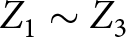 $Z_{1} \sim Z_{3}$ and electrical lengths
 $\theta_{1}$
 $\sim$
 $\theta_{3}$; a coupling capacitor
 $C_{g}$ between the stepped-impedance transmission lines; grounding parasitic capacitors
 $C_{1}$ and
 $C_{2}$ associated with the high-impedance lines; and inductors
 $L_{1}$
 $\sim$
 $L_{3}$. The values of the circuit components, extracted through curve fitting based on full-wave simulation results, are listed in Table 1.
(a) Layout of SIHTR (W1=0.1, Ls0=1.95, Ls1=1, Ls2=0.6, Ls3=2.2, Ls4=0.6, hp=0.25, S1=0.1, Ws1=0.825, Ws2=1.65, Ws3=2.475, hs1=0.83, hs2=0.63 (unit: mm)). (b) LC equivalent circuit of SIHTR. (c) LC and EM simulation results.

Figure 1 Long description
Stepped trace layout with dimension arrows and labels. A horizontal dimension at the top reads 4.15 and a vertical dimension at the right reads 3.05. Near the top, a shorter horizontal dimension is labeled Ls0 and a nearby vertical dimension is labeled hp. Along the upper trace, labels Ls1 and Ls2 appear beside dimension arrows and a label W1 appears inside the upper horizontal section. On the left side, a vertical dimension is labeled Ls4. In the lower portion, a stepped rectangular region is shown with two vertical dimension labels hs2 and hs1. Along the bottom, three horizontal width dimensions are labeled Ws1, Ws2 and Ws3 and a central gap dimension is labeled S1. A vertical dimension label Ls3 appears near the right side of the stepped region. LC circuit schematic drawn from Port1 at the left to Port2 at the right along a single top conductor. From the top conductor, two capacitors labeled C1 connect upward to ground symbols, one near Port1 and one near Port2. Two capacitors labeled C2 also connect upward to ground symbols, positioned between the C1 capacitors and closer to the center. Along the top conductor between the grounded capacitors, three series inductors are drawn and labeled L1, L2 and L1 from left to right. From two nodes on the top conductor near the center, two vertical inductors labeled L3 extend downward, one on the left side of the center and one on the right side of the center. The lower ends of these two L3 inductors connect to two vertical stacks of rectangular blocks. Between the two stacks, a capacitor labeled Cg is drawn horizontally, connecting the left stack to the right stack near their upper portions. The left stack contains three blocks labeled TL1, TL2 and TL3 from top to bottom, with text to the left reading Z1 comma theta1 near TL1, Z2 comma theta2 near TL2 and Z3 comma theta3 near TL3. The right stack contains three blocks labeled TL3, TL2 and TL1 from top to bottom, with text to the right reading Z3 comma theta3 near the top block, Z2 comma theta2 near the middle block and Z1 comma theta1 near the bottom block. Line plot of magnitude of S subscript 21 in decibel versus Frequency left parenthesis gigahertz right parenthesis. The horizontal axis is labeled Frequency left parenthesis gigahertz right parenthesis with tick labels 0, 10, 20, 30 and 40. The vertical axis is labeled vertical bar S subscript 21 vertical bar left parenthesis decibel right parenthesis with tick labels 0, minus 20, minus 40, minus 60, minus 80 and minus 100. Two curves are shown with a key at the lower right reading EM and LC. Two text labels, TZ1 near about 10 gigahertz and TZ2 near about 20 gigahertz, mark deep notches in the plotted response. The three parts are presented as a physical layout, a corresponding lumped element and transmission line schematic and a plotted magnitude response using the EM and LC traces.
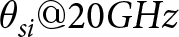

Table 1 Long description
Parameters are given for three capacitors labeled C1, C2, and Cg, three inductors labeled L1, L2, and L3, three impedances labeled Z1, Z2, and Z3, and three angles labeled theta 1, theta 2, and theta 3. C1 is 0.01 picofarads and C2 is 0.01 picofarads, while Cg is 0.18 picofarads. L1 is 0.93 nanohenries, L2 is 1.07 nanohenries, and L3 is 0.1 nanohenries. Z1 is 47.5 ohms, Z2 is 29 ohms, and Z3 is 20.86 ohms. Theta 1 is 27 degrees, theta 2 is 21 degrees, and theta 3 is 24.8 degrees.
As illustrated in Fig. 1(c), the simulated frequency response from the LC equivalent circuit exhibits excellent agreement with the full-wave electromagnetic (EM) simulation results, thereby validating the accuracy of the proposed circuit model. The simulated response indicates that the SIHTR achieves a 3 dB cut-off frequency at 8 GHz. In addition, two distinct transmission zeros (TZs) are observed at 9.21 GHz (TZ1) and 19.16 GHz (TZ2), respectively, which contribute to enhanced out-of-band rejection and improved filter selectivity.
Design of TSRs
To realize the LPF with an extended stopband, a modified TSR is proposed as the suppression cell, whose structure is shown in Fig. 2(a). For comparison, the conventional TSR structure is depicted in Fig. 2(b). The simulated responses of both (Fig. 2(c)) demonstrate that the proposed TSR achieves a significant performance enhancement, primarily characterized by a much wider stopband. Furthermore, the proposed TSR also affords a substantial reduction in layout area, occupying only approximately half that of its conventional counterpart. These results confirm the proposed TSR’s dual advantages in both performance and compactness.
(a) Layout of the proposed TSR (unit: mm). (b) Layout of conventional TSR (unit: mm). (c)  $|S_{21}|$ simulation comparison.

Figure 2 Long description
The A showing a dimensioned layout with two large rectangular blocks separated by a narrow horizontal gap and a central narrow connection. Four curved cutouts face the gap, two on the upper block and two on the lower block. Text labels near the left side read, Rs0 and Ws. A vertical dimension on the right reads, L2. A bottom horizontal dimension reads, 2.1. A right vertical dimension reads, 3.0. The B showing a dimensioned layout with two large rectangular blocks separated by a narrow horizontal gap and a central narrow connection. A bottom horizontal dimension reads, 2.9. A right vertical dimension reads, 4.2. The C showing a line graph with two curves and a legend. The x-axis label is, Frequency (gigahertz). The x-axis shows labeled ticks at 0, 20, 40 and 60. The y-axis label is, vertical bar S subscript 2 1 vertical bar (decibel). The y-axis shows labeled ticks at 0, minus 20 and minus 40. The legend lists two series: Conventional underscore TSR underscore Simulation and The underscore Proposed underscore TSR underscore Simulation. Conventional underscore TSR underscore Simulation starts near 0 decibel at 0 gigahertz, decreases to about minus 40 decibel near 30 gigahertz, then rises to about minus 20 decibel near 40 gigahertz. It continues with small undulations around the minus 20 to minus 10 decibel region from about 45 to 70 gigahertz. The underscore Proposed underscore TSR underscore Simulation starts near 0 decibel at 0 gigahertz, decreases to about minus 40 decibel near 30 gigahertz, then rises to about minus 20 decibel near 40 gigahertz. It shows a deeper dip near the high frequency region around the 60 gigahertz tick, reaching below minus 20 decibel, then rises toward the upper part of the plot by about 65 to 70 gigahertz.
The LC equivalent circuit of the proposed TSR is shown in Fig. 3(a). The inductors  $L_{0}$ and
 $L_{1}$, together with the parasitic ground capacitors
 $C_{1}$ and
 $C_{2}$, model the high-impedance transmission lines, while
 $C_{0}$ represents the capacitance of the open stubs.
(a) LC equivalent circuit of the proposed TSR. (b) Simulated results of the proposed TSR versus different Zs.

Figure 3 Long description
A circuit diagram with Port1 on the left and Port2 on the right. A top horizontal line connects Port1 to Port2. Near the left side of the top line, an inductor labeled L subscript 1 is placed in series. Near the right side of the top line, another inductor labeled L subscript 1 is placed in series. Four vertical branches connect from the top line down to a bottom horizontal line. From left to right, the first branch is a capacitor labeled C subscript 1. The second branch is a capacitor labeled C subscript 2. The third branch contains an inductor labeled L subscript 0 above a capacitor labeled C subscript 0. The fourth branch contains an inductor labeled L subscript 0 above a capacitor labeled C subscript 0. A ground symbol is connected to the bottom horizontal line below the two middle branches. A line graph with the horizontal axis labeled, Frequency left parenthesis gigahertz right parenthesis, with tick labels 0, 10, 20, 30, 40, 50, 60, 70. The vertical axis label is, vertical bar S subscript 21 vertical bar left parenthesis decibel right parenthesis, with tick labels 0, minus 20, minus 40. A label, f subscript 0, appears near the lowest point of the curves around 30 on the frequency axis. A legend lists five curves: Zs equals 20, Zs equals 40, Zs equals 60, Zs equals 80, Zs equals 100. All five curves start near 0 decibel at low frequency, drop to a minimum near minus 40 decibel at about 30 gigahertz, then rise toward higher frequencies. At 70 gigahertz, the curves are near 0 decibel, with the Zs equals 20 curve lowest among the five and the Zs equals 100 curve highest among the five.
Based on the LC equivalent circuit shown in Fig. 3(a), the resonant frequency  $f_0$ (corresponding angular frequency
 $\omega_{0}$) of the series resonator composed of the inductor
 $L_0$ and the capacitor
 $C_0$ is defined as:
 \begin{equation}
f_{0}=\frac{1}{2\pi\sqrt{L_{0}C_{0}}}
\end{equation}
 \begin{equation}
\omega_{0}=2\pi f_{0}
\end{equation}
Define an impedance:
 \begin{equation}
Zs=\sqrt{\frac{L_{0}}{C_{0}}}
\end{equation}
Then, the ABCD matrix of the TSR is expressed as:
 \begin{equation}\begin{bmatrix}A&B\\C&D\end{bmatrix}_{total}=\begin{bmatrix}A&B\\C&D\end{bmatrix}_{\pi_1}\cdot\begin{bmatrix}A&B\\C&D\end{bmatrix}_R\cdot\begin{bmatrix}A&B\\C&D\end{bmatrix}_{\pi_2}\end{equation}
Owing to the conversion relationship between S-parameters and ABCD parameters[Reference Pozar2]:
 \begin{equation}
S_{21}=\frac{2}{A+B/Z_{0}+CZ_{0}+D}
\end{equation}
Where  $Z_{0}$ denotes the characteristic impedance at the TSR input/output ports. According to formula (4):
 \begin{equation}|S_{21}|=\frac{1}{\sqrt{|A_1|^{2}+|A_2+A_3|^{2}}}
\end{equation}
 \begin{equation}
\begin{aligned}
A_1 &=(1-\omega^2 L_{1}C_{1})(1-\omega^2 L_{1}C_{2})-\omega L_{1}\left[\vphantom{\frac{2\omega \omega_{0}(1-\omega^2 L_{1}C_{1})}{(\omega_{0}^2-\omega^2)Zs}}\omega(C_{1}+\right.\\
&\quad \left.C_{2})-\omega^3 L_{1}C_{1}C_{2}+\frac{2\omega \omega_{0}(1-\omega^2 L_{1}C_{1})}{(\omega_{0}^2-\omega^2)Zs}\right]
\end{aligned}
\end{equation}
 \begin{equation}
A_{2}=\frac{\omega L_{1}}{Z_{0}}\left[(1-\omega^2 L_{1}C_{2})-\frac{\omega^2 \omega_{0}L_{1}}{(\omega_{0}^2-\omega^2)Zs}\right]
\end{equation}
 \begin{equation}
\begin{aligned}
A_{3} &=Z_{0}(1-\omega^2 L_{1}C_{1})\left[\vphantom{\frac{2\omega \omega_{0}(1-\omega^2 L_{1}C_{1})}{(\omega_{0}^2-\omega^2)Zs}}\omega(C_{1}+C_{2})-\omega^3 L_{1}C_{1}C_{2}\right.\\
&\quad \left.+\frac{2\omega \omega_{0}(1-\omega^2 L_{1}C_{1})}{(\omega_{0}^2-\omega^2)Zs}\right]
\end{aligned}
\end{equation}
As shown in formulas (6) $\sim$(9), increasing Zs raises
 $|S_{21}|$ near the resonant frequency
 $f_0$, indicating weaker suppression and a narrower stopband. Based on this, the inductance
 $L_{0}$ in the TSR’s LC model is calculated using formulas (1) and (3). Subsequently, the length variable
 $L_{2}$ (Ws=0.1mm) is estimated using the formula
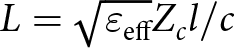 $L=\sqrt{\varepsilon_\mathrm{eff}}Z_cl/c$, where
 $Z_c$,
 $l$,
 $c$, and
 $\varepsilon_{eff}$ are the characteristic impedance, line length, speed of light, and effective dielectric constant, respectively. To ensure that the TSR achieves the desired resonant frequency
 $f_0$, the radius Rs0 was optimized accordingly. Figure 3(b) presents simulation results under different Zs values, confirming that larger Zs leads to reduced stopband bandwidth, consistent with theoretical predictions. Moreover, a higher Zs sharpens the transition from passband to stopband on the lower-frequency side of
 $f_0$, enhancing near-end out-of-band suppression.
Based on the above properties, two TSRs with distinct resonant frequencies are designed. TSR1, resonating at 15.25 GHz with a narrow stopband, improves near-stopband suppression, while TSR2, with a 30 GHz resonance and wide stopband, enhances far-stopband suppression. To reduce layout size, TSR1’s high-impedance line is folded. The optimized layouts and simulation results of TSR1 and TSR2 are shown in Fig. 4(a)–4(c).
(a) Layout of TSR1 (W1=0.1, Lt1=0.55, Lt2=0.45, Lt3=2Rs1=0.7, Lt4=0.2 (unit: mm)). (b) Layout of TSR2 (W2=0.1, Lt5=1.1, Lt6=3Rs2=1.12, Lt7=0.2 (unit: mm)). (c) Simulated results of TSR1. (d) Simulated results of TSR2.

Figure 4 Long description
A resonator layout with dimension arrows and labels, W1, Lt1, Lt2, Lt3, Lt4 and Rs1. A bottom horizontal dimension reads 3.10. A right vertical dimension reads 4.00. The image B showing a resonator layout with dimension arrows and labels, W2, Lt5, Lt6, Lt7 and Rs2. A bottom horizontal dimension reads 2.30. A right vertical dimension reads 2.96. The image C showing a line graph with two curves and a legend. The x-axis label is Frequency with unit gigahertz, with tick labels 0, 5, 10, 15, 20, 25, 30, 35, 40. The y-axis label is vertical bar S subscript 2 1 vertical bar with unit decibel, with tick labels 0, minus 10, minus 20, minus 30, minus 40, minus 50. The legend lists TSR1 Simulation and TSR2 Simulation. The TSR1 Simulation curve starts near 0 decibel at low frequency, drops to a minimum near the label f subscript o 1 around 15 gigahertz at about minus 50 decibel, then rises to about minus 20 decibel near 20 gigahertz, continues upward to near 0 decibel around 35 gigahertz and is slightly below 0 decibel near 40 gigahertz. The TSR2 Simulation curve starts near 0 decibel at low frequency, decreases gradually to about minus 10 decibel near 15 gigahertz, continues downward past minus 20 decibel near 25 gigahertz, reaches a minimum near the label f subscript o 2 around 30 gigahertz at about minus 40 decibel, then rises to about minus 25 decibel near 40 gigahertz.
Design of the proposed LPF
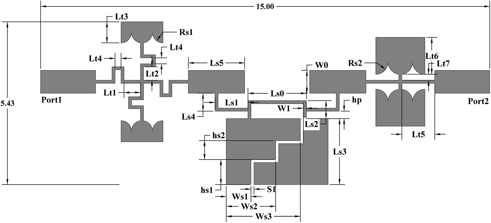
By integrating the SIHTR with TSR1 and TSR2, the final LPF layout is shown in Fig. 5, where two interconnect structures (ICSs) are introduced to connect the SIHTR and TSRs. In addition to providing electrical connectivity, these ICSs also serve as effective tuning elements for performance optimization. As shown in Fig. 6(a), adjusting the length of ICS section Ls5 effectively suppresses out-of-band spurious resonances. Modifying radius Rs1, as depicted in (Fig. 6(b)), enhances suppression in the near-end out-of-band region. Meanwhile, tuning Rs2 (Fig. 6(c)) improves the in-band  $|S_{11}|$ flatness and further strengthens near-stopband suppression. Figure 6(d) demonstrates that increasing width Ws2 results in a lower 3 dB cutoff frequency, with Ws1, Ws2, and Ws3 varying proportionally as Ws3 = 1.5Ws2 = 3Ws1.
The key structural parameters of the filter are obtained through optimization using the full-wave electromagnetic simulation software HFSS. Figure 7 compares the frequency responses of the LPF with and without the incorporation of TSRs. The results demonstrate that the inclusion of TSRs not only achieves a wider stopband and deeper attenuation but also significantly enhances the out-of-band interference rejection capability of the filter.
Layout of the proposed LPF (W0=0.76, W1=0.1, Ls0=1.95, Ls1=1, Ls2=0.6, Ls3=2.2, Ls4=0.6, Ls5=2.08, hp=0.25, S1=0.1, Ws1=0.825, Ws2=1.65, Ws3=2.475, hs1=0.83, hs2=0.63, Lt1=0.55, Lt2=0.45, Lt3=0.7,Lt4=0.2, Lt5=1.1, Lt6=1.23, Lt7=0.2, Rs1=0.35, and Rs2=0.41 (unit: mm)).

Figure 5 Long description
Port1 is on the left and Port2 is on the right, connected by a single main horizontal trace running left to right. A top dimension line across the full layout is labeled 15.00 and a left-side vertical dimension line is labeled 5.43. Starting at Port1, the main trace enters a wider rectangular section. Near this left section, several labeled features appear around the main line: Lt1 is marked near the left feed and a set of short vertical and horizontal trace segments form a stepped junction area. Above the main line, a U shaped trace feature is shown with labels Lt3 and Lt4 and a nearby label Rs1. Below the main line in the same left region, a similar U shaped trace feature is shown. Moving right along the main trace, a narrow section labeled Ls5 leads into another rectangular block on the main line. Below this mid region, a larger stepped rectangular area extends downward from the main line, with labels Ls4, Ls1 and Ls2 placed around the stepped sections. A narrow vertical gap or spacing is labeled hp near the main line and widths W0 and W1 are labeled on the main trace near this area. Additional width and spacing labels Ws1, Ws2, Ws3 and S1 are shown along the bottom of the downward stepped region, with vertical height labels hs1 and hs2 at the left side of that region. A vertical length label Ls3 is shown on the right side of the downward stepped region. Continuing right, the main trace passes through another rectangular section labeled Ls0 and then into a right-side structure near Port2. In this right region, two U shaped trace features are shown above and below the main line, with a nearby label Rs2. A vertical feature at the far right is labeled Lt6 and Lt7 and a nearby label Lt5 is shown near the lower right U shaped feature. The main trace terminates at Port2. Multiple additional labeled lengths and widths using the prefixes Lt and Ls are distributed around the stepped junctions and U shaped features, with no component values shown beyond the printed dimension labels.
(a) Simulated results of the proposed LPF versus different Ls5. (b) Simulated results of the proposed LPF versus different Rs1. (c) Simulated results of the proposed LPF versus different Rs2. (d) Simulated 3dB cutoff frequencies of the LPF under different Ws2.

Figure 6 Long description
Line graph with the y-axis label, vertical bar S subscript 2 1 vertical bar, in decibel and the x-axis label, Frequency, in gigahertz. The x-axis runs from 0 to 40. The y-axis runs from 0 to minus 80. A legend lists Ls5 equals 0.3 millimeter, Ls5 equals 0.9 millimeter, Ls5 equals 1.5 millimeter and Ls5 equals 2.1 millimeter. All curves stay near 0 decibel from 0 to about 8 to 9 gigahertz, then drop steeply to below minus 20 decibel near about 10 gigahertz. Between about 10 and 40 gigahertz, the curves show multiple dips and peaks. The deepest dip reaches about minus 80 decibel near about 15 to 16 gigahertz on the Ls5 equals 0.9 millimeter curve. Other curves show minima between about minus 60 and minus 75 decibel in the mid band and rise toward about minus 30 to minus 40 decibel in parts of the 30 to 40 gigahertz range. Line graph with the y-axis label, vertical bar S subscript 2 1 vertical bar, in decibel and the x-axis label, Frequency, in gigahertz. The x-axis runs from 2 to 12. The y-axis runs from 10 to minus 60. A legend lists Rs1 equals 0.20 millimeter, Rs1 equals 0.24 millimeter, Rs1 equals 0.28 millimeter, Rs1 equals 0.32 millimeter, Rs1 equals 0.36 millimeter and Rs1 equals 0.40 millimeter. All curves stay near 0 decibel from 2 to about 8 to 9 gigahertz, then drop sharply to a notch near about 9.5 to 10 gigahertz. The notch minima are around minus 50 to minus 55 decibel. After the notch, from about 10 to 12 gigahertz, the curves rise to between about minus 20 and minus 40 decibel, with the Rs1 equals 0.40 millimeter curve lowest near 12 gigahertz. Line graph with the y-axis label, Magnitude, in decibel and the x-axis label, Frequency, in gigahertz. The x-axis runs from 0 to 40. The y-axis runs from 0 to minus 100. Two legend groups are shown: Rs2 equals 0.30 millimeter minus S subscript 2 1, Rs2 equals 0.36 millimeter minus S subscript 2 1 and Rs2 equals 0.42 millimeter minus S subscript 2 1; and Rs2 equals 0.30 millimeter minus S subscript 1 1, Rs2 equals 0.36 millimeter minus S subscript 1 1 and Rs2 equals 0.42 millimeter minus S subscript 1 1. The S subscript 2 1 curves stay near 0 decibel up to about 9 to 10 gigahertz, then drop below minus 20 decibel and show multiple dips between about 10 and 40 gigahertz, including a deep minimum near about 22 to 24 gigahertz reaching about minus 80 to minus 90 decibel. The S subscript 1 1 curves appear between about minus 10 and minus 30 decibel at lower frequencies, then change sharply near about 9 to 10 gigahertz and continue with variations across the band, including a dip near the low 20 gigahertz region and a rise toward about minus 30 to minus 40 decibel near about 30 gigahertz. Line graph with the y-axis label, vertical bar S subscript 2 1 vertical bar, in decibel and the x-axis label, Frequency, in gigahertz. The x-axis runs from 6 to 14. The y-axis runs from 0 to minus 60. A legend lists Ws2 equals 1.55 millimeter, Ws2 equals 1.65 millimeter and Ws2 equals 1.75 millimeter. All curves stay near 0 decibel from 6 to about 8 to 9 gigahertz, then drop steeply to a notch near about 9 to 10 gigahertz with minima around minus 45 to minus 55 decibel. After the notch, the curves rise to around minus 30 to minus 35 decibel near about 10 gigahertz and then slope downward toward about minus 45 decibel by 14 gigahertz.
Simulated S-parameters.

Fabrication and measurement of the proposed filter
Finally, the proposed LPF is fabricated on a Rogers RT/Duroid 5880 substrate with a size of 11.3mm  $\times$ 5.43mm, a thickness of 0.254mm, and a dielectric constant of 2.2. For ease of measurement, two solderless SMA connectors (2.92-KFD0851) are mounted at the input and output ports of the fabricated LPF. The photograph of the fabricated LPF is presented in Fig. 8(a), while the measured S-parameters, obtained using an AV3672C vector network analyzer, are depicted in Fig. 8(b). These measurements validate the performance of the proposed design and are used for comparison with the simulated results.
(a) Fabricated the proposed LPF. (b) Measurement and simulation.

Figure 8 Long description
A rectangular circuit board held between two metal end blocks with threaded coaxial connectors on the left and right. Four screws are visible, two near the left end and two near the right end. A coin marked, 1 and 2014 is placed above the board. A conductive trace pattern is visible on the board surface. The image B showing a line graph with four curves and a legend listing, S11 simulation, S21 simulation, S11 measurement and S21 measurement. The x-axis label is, Frequency gigahertz, with tick labels at 0, 5, 10, 15, 20, 25, 30, 35 and 40. The y-axis label is, Magnitude decibel, with tick labels at 0, minus 20, minus 40, minus 60 and minus 80. A dashed horizontal line is drawn at minus 30 decibel. Text near the dashed line reads, Stop Band 9.17 to 40 gigahertz. A marked point near the upper left region is labeled, 8.23, minus 3. Another marked point near the right side is labeled, 31.7, minus 31.5. The S11 simulation curve stays close to 0 decibel from 0 to 40 gigahertz with small dips, including a dip around the low single digit gigahertz region and additional shallow dips in the low to mid 30 gigahertz region. The S11 measurement curve shows a deep notch near about 5 gigahertz reaching below minus 40 decibel, then rises toward 0 decibel by around 9 to 10 gigahertz and remains near 0 decibel with small variations through 40 gigahertz. The S21 simulation curve is near 0 decibel up to around 9 gigahertz, then drops below minus 30 decibel after about 10 gigahertz. It reaches a low point around the low 20 gigahertz region near about minus 70 decibel, then rises toward about minus 35 decibel near the low 30 gigahertz region and shows a sharp narrow dip in the mid 30 gigahertz region before ending near about minus 45 decibel at 40 gigahertz. The S21 measurement curve is near 0 decibel up to around 9 gigahertz, then drops below minus 30 decibel after about 10 gigahertz. It varies between about minus 35 and minus 65 decibel from about 10 to 30 gigahertz, rises to a peak near the labeled point 31.7, minus 31.5, then drops again with multiple notches in the mid to high 30 gigahertz region, including a deep notch below minus 70 decibel near the high 30 gigahertz region and ends below minus 40 decibel at 40 gigahertz.
The measured results indicate that the proposed LPF exhibits an insertion loss of less than 1 dB and a return loss better than 15.1 dB across the DC to 7.5 GHz passband. The sharpness parameter  $\zeta$ is given by Equation (10) [Reference Roshani, Yahya, Khazaei, Roshani and Karami10].
 \begin{equation}
\zeta=\frac{\alpha_{max}-\alpha_{min}}{f_s-f_c}
\end{equation}
Where  $\alpha_{max}$ = 40 dB at
 $f_s$ = 9.3 GHz and
 $\alpha_{min}$ = 3 dB at
 $f_c$ = 8.23 GHz represent the attenuation levels of the
 $S_{21}$ parameter. The sharpness parameter of the proposed filter is 34.58 dB/GHz.
Using equations (11) and (12)[Reference Roshani, Yahya, Khazaei, Roshani and Karami10], the suppression factor (SF) and related stopband bandwidth (RSB) are determined.
 \begin{equation}
\mathrm{SF}=\frac{rejection\;level\;in\;stopband}{10}
\end{equation}
 \begin{equation}
\mathrm{RSB}=\frac{stopband(20dB\;attenation\;level)}{stopband\;centre\;frequency}
\end{equation}
 \begin{equation}
\mathrm{NCS}=\frac{physical\;size(length\times width)}{\lambda_g^{2}}
\end{equation}
The designed filter exhibits a wide stopband ranging from 9.17 to 40 GHz, achieving an attenuation greater than 31.5 dB. This performance corresponds to an SF parameter of 3.15 and an RSB parameter of 1.27, as calculated from equations (11) and (12), respectively. Furthermore, the normalized circuit size(NCS) is determined using equation (13) [Reference Roshani, Yahya, Khazaei, Roshani and Karami10], where the waveguide length  $\lambda_g $ is evaluated at 8.23 GHz. Table 2 shows the comparison between the proposed LPF with the reported ones.
Performance comparisons between the proposed filter and other works

Table 2 Long description
Rows compare references 4 through 10 and, This work, across five columns: center frequency in gigahertz, NCS in lambda g squared, zeta in decibels per gigahertz, SF, and RSB. Reference 4 lists 1.57 gigahertz, NCS 0.01035, zeta 170, SF 2, RSB 1.59. Reference 5 lists 1.08 gigahertz, NCS 0.01795, zeta 81, SF 2.11, RSB 1.65. Reference 6 lists 1.95 gigahertz, NCS 0.03357, zeta 440, SF 1.5, RSB 1.56. Reference 7 lists 1.12 gigahertz, NCS 0.0101, zeta 201, SF 2.2, RSB 1.7. Reference 8 lists 1.93 gigahertz, NCS 0.01955, zeta 425, SF 2, RSB 1.65. Reference 9 lists 2.15 gigahertz, NCS 0.0132, zeta 123, SF 2, RSB 1.6. Reference 10 lists 1.61 gigahertz, NCS 0.009, zeta 99.44, SF 2, RSB 1.49.
Conclusion
A high-performance microstrip LPF is proposed by integrating an SIHTR with a pair of asymmetric TSRs. Lumped-element equivalent circuit models of the SIHTR and TSRs are developed to analyze their respective characteristics and advantages. Building upon the low-pass response established by the SIHTR, the TSRs are incorporated to further enhance near-stopband suppression and to broaden the overall stopband bandwidth. The measured results show good agreement with full-wave electromagnetic simulations, confirming that the proposed filter achieves a compact structure, sharp roll-off, wide stopband, high return loss, and excellent stopband attenuation performance. In consideration of these specifications, the proposed LPF demonstrates suitability for integration into broadband spread-spectrum modules.
Acknowledgements
This work was supported in part by the Chongqing Natural Science Foundation under Grant CSTB2022NSCQ-MSX1521.
Competing interests
The authors declare none.

Shuhang Chen was born in Pengzhou, Sichuan, China, in 1997. He received the B.E. degree in Electronic Information Engineering from Southwest Petroleum University, Chengdu, China, in 2021, and the M.S. degree in Electronic Information from the School of Aeronautics and Astronautics, University of Electronic Science and Technology of China, Chengdu, China, in 2025. His current research interests include RF passive devices and metamaterials.

Wentao Pan was born in Zhongwei, Ningxia, in 2001. He is currently pursuing a master’s degree at the University of Electronic Science and Technology of China. His main research interests are RF microwave circuits design and antenna design.

Kai Yang received the B.S. degree in electronic science and technology and the master’s degree in circuits and systems from the University of Electronic Science and Technology of China (UESTC), Chengdu, China, in 1993 and 2000, respectively. In 2001, he was promoted as an Associate Professor with UESTC, where he was promoted as a Full Professor in 2007. In 2002, he was selected as the Academic Outstanding Young Scientist Leader Training Plan of Sichuan Province. In 2003, he was a Member of the National Superconducting Standardization Technology Committee. In 2006, he was selected as a Senior Member of the Chinese Institute of Electronics (CIE). He has authored or coauthored more than 50 papers in international and domestic journals and conferences. His current research interests include high-temperature superconducting circuits and systems, and RF and microwave passive circuits.




 Open access

