2.1 EPF modelling for point objects

If there are N point objects in the two-dimensional (2D) plane and an i-th ($i = 1,2, \cdots ,N$) object with position ${p_i}({x_i},{y_i})$, the distance between any position $p(x,y)$ and ${p_i}$ is ${f_{\textrm{Po}{\mathop{\rm int}} - i}} = \sqrt {{{({x - {x_\textrm{i}}} )}^2} + {{({y - {y_\textrm{i}}} )}^2}}$, and the potential field at location $p(x,y)$ can be written as:

(1)\begin{equation}{\boldsymbol{f}_{\textbf{Point}}}(\boldsymbol{p}) = \sum\limits_{\boldsymbol{i}\mathbf{=}\mathbf{1}}^{\boldsymbol{N}} {\frac{\mathbf{1}}{{\mathbf{1}\mathbf{+}{\textbf{e}^{{\boldsymbol{\beta}_{\boldsymbol{i}}}{\,\boldsymbol{f}_{\textbf{Point} - \boldsymbol{i}}}}}}}}\end{equation}

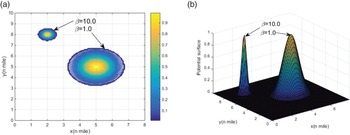
where ${\boldsymbol{\beta}_{\boldsymbol{i}}}$ is the i-th positive parameter of the point object; the larger the value of ${\boldsymbol{\beta}_{\boldsymbol{i}}}$, the steeper the potential field and the smaller the action range. Otherwise, the smaller the value of ${\boldsymbol{\beta}_{\boldsymbol{i}}}$, the flatter the potential field and the larger the action range. Figure 1 shows the different action ranges and potential surfaces for different ${\boldsymbol{\beta}_{\boldsymbol{i}}}$. The potential field reaches the maximum value of 1 ⋅ 0 at position ${p_i}({x_i},{y_i})$ and approaches 0 ⋅ 0 at positions far away from ${p_i}({x_i},{y_i})$.

Figure 1.

Potential field for point objects with different values of ${\boldsymbol{\beta}_{\boldsymbol{i}}}$: (a) potential contours, (b) potential surfaces

2.2 EPF modelling for line objects

Line objects provided by the electronic chart are represented by a group of line segments. Among the anticlockwise sorted line segments, if the i-th line segment $\mathop {{p_i}{p_{i + 1}}}\limits^ \to$ starts from ${p_i}({x_i},{y_i})$ and ends at ${p_{i + 1}}({x_{i + 1}},{y_{i + 1}})$, then the implicit function of the line segment is ${f_{\textrm{Line - }i}} = {A_i}x + {B_i}y + {C_i}$. For any point $p(x,y)$, it is on the line when ${f_{\textrm{Line - }i}} = 0$, or on the left side of the line when${f_{\textrm{Line - }i}} > 0$, or on the right side of the line when ${f_{\textrm{Line - }i}} < 0$. The potential field of the line object can be expressed as:

(2)\begin{equation} {\boldsymbol{f}_{\textbf{Line}}}(\boldsymbol{p}) = \sum\limits_{\boldsymbol{i} \mathbf{=} \mathbf{1}}^{\boldsymbol{N}} \frac{\mathbf{1}}{{\mathbf{1} \mathbf{+} {\textbf{e}^{-{\boldsymbol{\gamma}_{\boldsymbol{i}}{\,\boldsymbol{f}_{\textbf{Line-}\boldsymbol{i}}}}}}}}\end{equation}

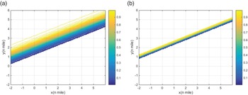
where ${\boldsymbol{\gamma}_{\boldsymbol{i}}}$ is the i-th positive parameter of the line segment that determines the influence range of the line; the smaller the value of ${\boldsymbol{\gamma}_{\boldsymbol{i}}}$ means the flatter the potential field and the larger the action range of the line; otherwise, a larger value of ${\boldsymbol{\gamma}_{\boldsymbol{i}}}$ means a steeper potential field and a smaller action range of the line. As shown in Figure 2, when ${f_{\textrm{Line - }i}} = 0$, the point $p(x,y)$ is on the line segment, and the potential field value is 0 ⋅ 5. If ${f_{\textrm{Line - }i}} > 0$, the potential field value is larger, and the maximum is 1 ⋅ 0. If ${f_{\textrm{Line - }i}} < 0$, the potential field value is smaller, and the minimum value is 0.

Figure 2.

Potential fields for line objects: (a) ${\boldsymbol{\gamma}_{\boldsymbol{i}}}\textrm{ = }1.0$, (b) ${\boldsymbol{\gamma}_{\boldsymbol{i}}}\textrm{ = 5}.0$

2.3 EPF modelling for face objects

If there are N face objects in the 2D plane, then each face object is represented by a group of anticlockwise sorted line segments. If we can obtain the mathematical expression ${F_i}(x,y)$ of the face object and let the points inside the polygon fulfil the expression ${F_i}(x,y) < 0$, let points on the edge fulfil the expression ${F_i}(x,y) = 0$, and let points outside the polygon fulfil the expression ${F_i}(x,y) > 0$, then the potential field of face object can be expressed as:

(3)\begin{equation}{\boldsymbol{f}_{\textbf{face}}}(\boldsymbol{p}) = \sum\limits_{\boldsymbol{i} \mathbf{=} \mathbf{1}}^{\boldsymbol{N}} {\frac{\mathbf{1}}{{\mathbf{1} \mathbf{+} {\textbf{e}^{-{\boldsymbol{\alpha}_{\boldsymbol{i}}}{\boldsymbol{F}_{\boldsymbol{i}}}(\boldsymbol{x},\boldsymbol{y})}}}}}\end{equation}

where ${\boldsymbol{\alpha}_{\boldsymbol{i}}}$ is the positive parameter of the i-th face object. Similarly, the smaller the value of ${\boldsymbol{\alpha}_{\boldsymbol{i}}}$, the flatter the potential field and the larger the action range of the face object. Otherwise, the larger the value of ${\boldsymbol{\alpha}_{\boldsymbol{i}}}$, the steeper the potential field and the smaller the action range of the face. If ${F_i}(x,y) = 0$, point $p(x,y)$ is on the edge of the face object, and the potential field value is 0 ⋅ 5. If ${F_i}(x,y) > 0$, $p(x,y)$ is outside the face object, then the potential field value is smaller, and the minimum is 0. If ${F_i}(x,y) < 0$, $p(x,y)$ is inside the face object, the potential field value is larger, and the maximum is 1 ⋅ 0.

A MASS should maintain a safe distance from islands or shallow waters when navigating. However, sometimes it is required to navigate inside certain navigable regions and maintain a safe distance from the edges of the region, such as navigating in channels, traffic separation schemes, or other safe navigable areas. The potential field of the face object can be expressed as:

(4)\begin{equation} {\boldsymbol{f}_{\textbf{face-}\boldsymbol{i}}}\mathbf{=}\mathbf{1}-\frac{\mathbf{1}}{{\mathbf{1} \mathbf{+} {\textbf{e}^{-{\boldsymbol{\alpha}_{\boldsymbol{i}}}{\boldsymbol{F}_{\boldsymbol{i}}}(\boldsymbol{x},\boldsymbol{y})}}}}\end{equation}

where the inside of the face is navigable, the potential field is smaller, and the minimum is 0; whereas the outside of the face is unnavigable, and the potential field approaches 1 ⋅ 0 if it is far away from the face object.

2.4 EPF of the entire static environment

If there are M, N, and Q point objects, line objects, and face objects around the MASS, respectively, then the total potential field of the entire static environment can be obtained by adding the potential field generated by the point objects, line objects, and face objects. The environmental potential field at $p(x,y)$ can then be expressed as:

(5)\begin{equation} \boldsymbol{f}(\boldsymbol{p}) = {\boldsymbol{f}_{\textbf{face}}}(\boldsymbol{p})\mathbf{+} {\boldsymbol{f}_{\textbf{Line}}}(\boldsymbol{p}) \mathbf{+}{\boldsymbol{f}_{\textbf{Point}}}(\boldsymbol{p})\end{equation}

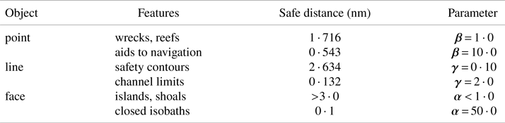
Each spatial object has a unique attribute for navigation. By setting the appropriate values for $\boldsymbol{\beta}$, $\boldsymbol{\gamma}$, and $\boldsymbol{\alpha}$ to specify the action ranges of the object, the recommended parameter for each spatial object and the safe distance to be maintained are listed in Table 1.

Table 1.

Recommended $\boldsymbol{\beta}$, $\boldsymbol{\gamma}$, and $\boldsymbol{\alpha}$ values for different objects

3.1 Theory of R-function

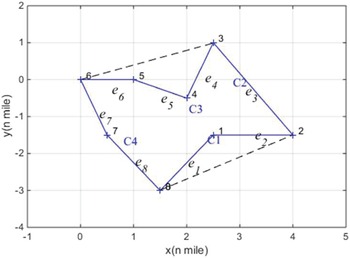
For the geometry in the 2D plane (as shown in Figure 3), the equation for each edge can be expressed by an implicit function ${f_i}(x,y) = 0$. The implicit function separates the plane into two half-spaces. The points on the line fulfil the expression of ${f_i}(x,y) = 0$, and the points in the half-space fulfil the expression of ${f_i}(x,y) > 0$ or ${f_i}(x,y) < 0$. For an arbitrary closed shape, if the vertices are sorted anticlockwise, the inner part of the shape can be expressed by the left half-space of each edge (${f_i}(x,y) < 0$). Therefore, the R-function can be used to express the region enclosed by two inequalities as function operations; through algebra operations to the implicit function of each edge, we can obtain the expressions $F(x,y) < 0$, $F(x,y) = 0$, and $F(x,y) > 0$ to express that point $p(x,y)$ is internal, boundary, or external to the geometric object.

Figure 3.

Convex hull and side-chains of polygon B

The R-function is a real-value function characterised by a property that is completely determined by the sign of its arguments rather than its value. Rvachev presented a series of useful R-functions with sufficient completeness, where ${R_a}$ is an R-function system:

(6)\begin{equation}{R_a} = \frac{1}{{1 + a}}(x + y \pm \sqrt {{x^2} + {y^2} - 2axy}) \end{equation}

where $a = a(x,y)$ is an arbitrary continuous and symmetric function and fulfilled by the expression $- 1 < a(x,y) \le 1$. The symbol ${\pm}$ denotes the R-conjunction and R-disjunction. If $a = 0$ or $a = 1$, the widely used ${R_0}$ system and ${R_1}$ system are as follows:

(7)\begin{gather}{R_0} = x + y \pm \sqrt {{x^2} + {y^2}}\end{gather}

(8)\begin{gather}{R_1} = x + y \pm |{x - y} |\end{gather}

Compared with other R-function systems, the ${R_0}$ system is differentiable except at the origin, and the calculation is simple. In this study, we select the ${R_0}$ system to represent the geometric objects.

The implicit function based on the aforementioned approach cannot accurately calculate the signed distance between a space point and an object boundary, so normalised function was introduced into the geometric object expression. For line segments expressed as ${f_{\textrm{Line - }i}} = {A_i}x + {B_i}y + {C_i}$, its normalised function is:

(9)\begin{equation}{f_{\textrm{Line - }i}} = \frac{{{A_i}}}{Q}x + \frac{{{B_i}}}{Q}y + \frac{{{C_i}}}{Q},\quad Q = \sqrt {{A_i}^2 + {B_i}^2}\end{equation}

3.2 R-function representation for geometric objects

Arbitrary geometric objects can be expressed by several basic primitives through regular Boolean operations (‘intersection’ or ‘union’). The geometric object B can be expressed in the following form:

(10)\begin{equation}B = F[{{B_1},{B_2}, \cdots ,{B_n}} ]\end{equation}

where ${B_i}$($i = 1,2, \cdots ,n$) is a basic primitive and F is a regular Boolean function with operations of ${ \cap ^\ast }$, ${ \cup ^\ast }$, and ${ - ^\ast }$. If the logical operations ${\wedge}$, ${\vee}$, and $\neg$ are used to displace the Boolean operations, then F becomes a logical function. Combined with the definition of the R-function, the geometric object B can be expressed as follows:

(11)\begin{equation}F[{S({B_1}),S({B_2}), \cdots ,S({B_n})} ]= 1\end{equation}

where the basic primitive ${B_i}$ is the half-space of the geometric object expressed by an implicit function ${f_i}(x) \le 0$. If the signed distance function ${f_i}(x)$ for basic primitive ${B_i}$ is:

(12)\begin{equation}{B_i}:{f_i}(x) \ge 0\quad (i = 1,2, \cdots ,n)\end{equation}

then Equation (10) can be written as:

(13)\begin{equation}F[{S({f_1}),S({f_2}), \cdots ,S({f_n})} ]= 1\end{equation}

According to Equation (13), given a continuous function $f(x)$ and its correlation function $F({X_1},{X_2}, \cdots ,{X_n})$, the geometric object B can be expressed as:

(14)\begin{equation}f({f_1},{f_2}, \cdots ,{f_n}) \ge 0\end{equation}

where ${f_i}(i = 1,2, \cdots ,n)$ is a real continuous function, and f is the implicit function of B. Because the geometric objects in this study are all in the 2D plane and without any curves or surfaces, the implicit function of the geometric object is accurate for expressing the object. Otherwise, the implicit function approximately expresses the geometric object.

3.3 Discrete-convex hull method

The expression of the geometric object using R-function is a semi-analytical solution based on its constructive solid geometry(CSG) model, and the implicit function can be used to accurately express the geometric object in the 2D plane. CSG representations usually have various logical and implicit functions, but they have the same logical functionality. In fact, the automatic generation of a CSG representation for an overly complex object is an intractable task. However, existing algorithms can automatically generate the CSG representations for polygonal regions. A polygonal region can be automatically divided into side-chains with the intersection of convex hull vertices. The intersection of the half-space defined by side-chains can then be adopted to express a polygonal region, whereas the half-space is represented by the intersection or union of the edges. If the intersection of the two edges is concave, the half-space is the union; otherwise, it is the intersection. The region B shown in Figure 3 has the logical function $B = {C_1} \wedge {C_2} \wedge {C_3} \wedge {C_4}$. Here, ${C_1} = {e_1} \vee {e_2}$,${C_2} = {e_3}$,${C_3} = {e_4} \vee ({e_5} \wedge {e_6})$ and ${C_4} = {e_7} \wedge {e_8}$.

The aforementioned approach for dealing with a geometric object is referred to as the discrete-convex hull method. As mentioned previously, the face objects in this study are represented by a group of anticlockwise sorted line segments in the 2D plane; their implicit functions are accurate for expressing geometric objects. Therefore, the implicit function of a geometric object has a value of 0 at the boundary of the object, and the internal and external points have values <0 and >0, respectively.

3.4 EPF modelling procedure for complex face object

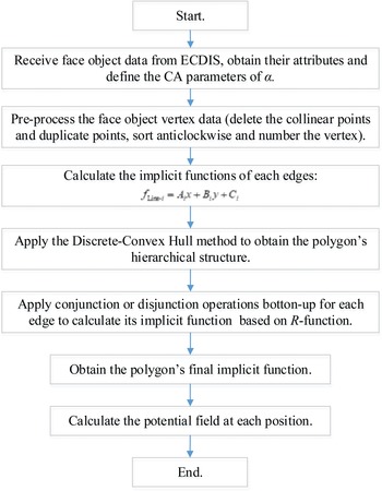
The procedure of EPF modelling for complex face objects can be summarised as follows (as shown in Figure 4). First, data on the face objects are received from ECDIS, the attributes are obtained, and the CA parameters of $\alpha$ are defined to specify their action ranges. Second, the vertices of the face objects are pre-processed, including deleting collinear or duplicate points, sorting anticlockwise, and numbering. Third, the implicit functions of each edge were calculated, and the discrete-convex hull method is applied to obtain the hierarchical structure of the polygon. Fourth, the conjunction or disjunction operation is applied bottom-up for each edge to obtain an implicit function based on the R-function. Finally, the implicit function of the polygon is obtained, and the potential field at each position is calculated.

Figure 4.

EPF modelling procedure for complex face object

4.1 Modelling of motions of MASS

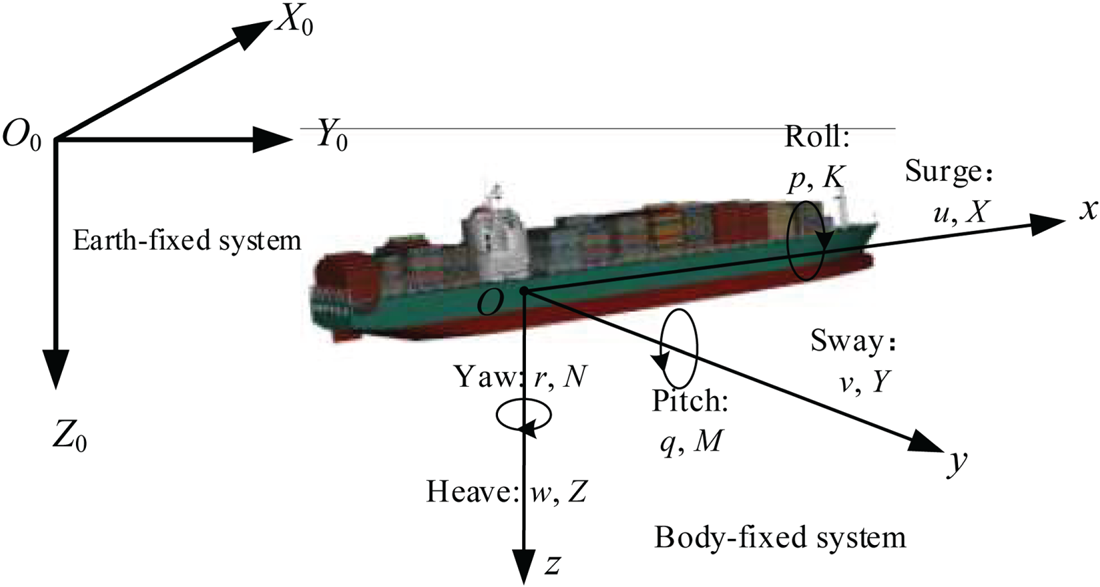
To describe the motion of a MASS in CA, the Earth- and body-fixed coordinate systems were constructed as shown in Figure 5. The vector $\boldsymbol{\eta} = {[{x,y,z,\phi ,\theta ,\psi } ]^\textrm{T}}$ represents the position and altitude of MASS in the Earth-fixed system, and the vector $\boldsymbol{\nu} = {[{u,v,w,p,q,r} ]^\textrm{T}}$ represents the speed and rotation speed in the body-fixed system. The 6-DOF mathematical model of the MASS can be expressed as:

(15)\begin{equation}\left\{ \begin{array}{@{}l} ({m\textrm{ + }{m_x}} )\dot{u} - ({m + {m_y}} )vr + ({m + {m_z}} )wq = {X_H} + {X_G} + {X_P} + {X_R} + {X_{\textrm{Env}}}\\ ({m\textrm{ + }{m_y}} )\dot{v} + ({m + {m_x}} )ur - ({m + {m_z}} )wp = {Y_H} + {Y_G} + {Y_P} + {Y_R} + {Y_{\textrm{Env}}}\\ ({m\textrm{ + }{m_z}} )\dot{w} - ({m + {m_x}} )uq + ({m + {m_y}} )vp = {Z_H} + {Z_G} + {Z_P} + {Z_R} + {Z_{\textrm{Env}}}\\ ({{I_{xx}} + {J_{xx}}} )\dot{p} + ({I_{zz}} + {J_{zz}} - {I_{yy}} - {J_{yy}})qr + ({{m_z} - {m_y}} )vw = {K_H} + {K_G} + {K_P} + {K_R} + {K_{\textrm{Env}}}\\ ({{I_{yy}} + {J_{yy}}} )\dot{q} + ({I_{xx}} + {J_{xx}} - {I_{zz}} - {J_{zz}})pr + ({{m_x} - {m_z}} )uw = {M_H} + {M_G} + {M_P} + {M_R} + {M_{\textrm{Env}}}\\ ({{I_{zz}} + {J_{zz}}} )\dot{r} + ({I_{yy}} + {J_{yy}} - {I_{xx}} - {J_{xx}})pq + ({{m_y} - {m_x}} )uv = {N_H} + {N_G} + {N_P} + {N_R} + {N_{\textrm{Env}}} \end{array} \right.\end{equation}

where $m = {\rho _s}\nabla$ represents the mass of the vessel; ${\rho _s}$ is the seawater density; $\nabla$ is the displacement; ${m_x}$, ${m_y}$, and ${m_z}$ denotes the mass added to the vessel; ${I_{xx}}$, ${I_{yy}}$, ${I_{zz}}$, ${J_{xx}}$, ${J_{yy}}$, ${J_{zz}}$ denote the moments and added moments of inertia; the subscripts H and G represent the viscous hydrodynamics and hydrostatic forces exerted on the naked hull; the subscripts P and R are the forces and moments generated by the propeller and rudder; the subscript ‘Env’ denotes the external disturbance forces induced by wind, wave, and current.

Figure 5.

Coordinate system of ship motion

4.2 Modified APF model

The attractive ${F_{\textrm{att}}}$ and repulsive ${F_{\textrm{rep}}}$ forces exerted on the ship under varying conditions were established by referring to the work of Lyu and Yin (Reference Lyu and Yin2018a, Reference Lyu and Yin2019a). Because of the numerous and undefined parameters for CA, the CA results have no direct relationship with the CA parameters, and the cited work of Lyu and Yin is therefore incomprehensible and unacceptable for navigators. As the DCPA-TCPA is the essential criterion rule for ‘risk of collision’ in navigation, we modified the negotiation CA repulsive force ${F_{\textrm{rd}}}$ and emergency CA repulsive force ${F_{\textrm{re}}}$ as follows:

(16)\begin{equation}{F_{\textrm{att}}} = \varepsilon {d_{\textrm{og}}}\overrightarrow {{n_{\textrm{og}}}}\end{equation}

(17)\begin{equation}{F_{\textrm{rep}}}(p,v) = \left\{\begin{array}{@{}lll} {{F_{\textrm{rd1}}} + {F_{\textrm{rd2}}}+ {F_{\textrm{rd3}}},} & {\textrm{if }{d_{\textrm{emg}}} < d \le {d_{\textrm{neg}}},} & {\theta < {\theta_m },0 \le {d_{\textrm{CPA}}} \le d\textrm{TO}{\textrm{L}_{\textrm{neg - CPA}}},}\\ & & {0 \le {t_{\textrm{CPA}}} \le t\textrm{TO}{\textrm{L}_{\textrm{neg - CPA}}}}\\ {{F_{\textrm{re1}}}+ {F_{\textrm{re2}}} + {F_{\textrm{re3}}},} & {\textrm{if }d \le {d_{\textrm{emg}}},} & {0 \le {\textrm{d}_{\textrm{CPA}}} \le d\textrm{TO}{\textrm{L}_{\textrm{emg - CPA}}},}\\ & & {0 \le {t_{\textrm{CPA}}} \le t\textrm{TO}{\textrm{L}_{\textrm{emg - CPA}}}}\\ \textrm{0}& {\textrm{otherwise}}& {}\end{array} \right.\end{equation}

(18)\begin{align} & {\boldsymbol{F}_{\textrm{rd1}}} ={-} {\eta _d}{d_g}^2\nonumber\\ & \left[ \left( {\dfrac{1}{{d - {d_{\textrm{emg}}}}} - \dfrac{1}{{{d_{neg}} - {d_{\textrm{emg}}}}}} \right){e^{{\theta_m} - \theta }}\left( {\dfrac{{d\textrm{TO}{\textrm{L}_{\textrm{neg - CPA}}}}}{{d\sqrt {{d^2} - {d_{\textrm{emg}}}^2} }} + \dfrac{{\sin \theta }}{{||{{\boldsymbol{v}_{ot}}} ||}}} \right) + \dfrac{{{e^{{\theta_m} - \theta }} - 1}}{{{{(d - {d_{\textrm{emg}}})}^2}}}\right.\nonumber\\ & \left.\quad - \left({\dfrac{1}{{d - {d_{\textrm{emg}}}}} - \dfrac{1}{{{d_{neg}} - {d_{\textrm{emg}}}}}} \right)\left( {\dfrac{{{d_{\textrm{emg}}}}}{{d\sqrt {{d^2} - {d_{\textrm{emg}}}^2} }} + \dfrac{{\sin {\theta_m}}}{{||{{\boldsymbol{v}_{ot}}} ||}}} \right) \right]{{\boldsymbol n}_{ot}} \end{align}

(19)\begin{align} & {\boldsymbol{F}_{\textrm{rd2}}} ={\pm} {\eta _d}{d_g}^2\nonumber\\ & \left[ \left( {\dfrac{1}{{d - {d_{\textrm{emg}}}}} - \dfrac{1}{{{d_{neg}} - {d_{\textrm{emg}}}}}} \right){e^{{\theta_m} - \theta }}\left( {\dfrac{1}{{||{{\boldsymbol{p}_{ot}}} ||}} + \dfrac{{\cos \theta }}{{||{{\boldsymbol{v}_{ot}}} ||}}} \right) + \dfrac{{||{{\boldsymbol{v}_{ot \bot }}} ||({e^{{\theta_m} - \theta }} - 1)}}{{d{{(d - {d_{\textrm{emg}}})}^2}}}\right.\nonumber\\ & \quad\left.- \left( {\dfrac{1}{{d - {d_{\textrm{emg}}}}} - \dfrac{1}{{{d_{neg}} - {d_{\textrm{emg}}}}}} \right)\left( {\dfrac{1}{{||{{\boldsymbol{p}_{ot}}} ||}} + \dfrac{{\cos {\theta_m}}}{{||{{\boldsymbol{v}_{ot}}} ||}}} \right) \right]{\boldsymbol{n}_{ot \bot }} \end{align}

(20)\begin{equation}{\boldsymbol{F}_{\textrm{rd3}}} = {\eta _d}{d_g}\left( {\frac{1}{{d - {d_{\textrm{emg}}}}} - \frac{1}{{{d_{neg}} - {d_{\textrm{emg}}}}}} \right)({e^{{\theta _m} - \theta }} - 1){\boldsymbol{n}_{og}}\end{equation}

(21)\begin{equation}{\boldsymbol{F}_{\textrm{re1}}} ={-} \textrm{2}{\eta _\textrm{e}}{d_g}^2\left[ {\left( {\left. {\frac{1}{{d\textrm{ - }d\textrm{TO}{\textrm{L}_{\textrm{emg - CPA}}}}} - \frac{1}{{{d_{\textrm{emg}}}}}} \right)} \right. \times \frac{1}{{{{({d\textrm{ - }d\textrm{TO}{\textrm{L}_{\textrm{emg - CPA}}}} )}^2}}}\textrm{ + }||{{\boldsymbol{v}_{ot}}} ||\cos \theta } \right]{\boldsymbol{n}_{ot}}\end{equation}

(22)\begin{equation}{\boldsymbol{F}_{\textrm{re2}}} = 2{\eta _\textrm{e}}\frac{{{d_g}^2}}{d}({||{{\boldsymbol{v}_{ot}}} ||^2}\cos \theta \sin \theta ){\boldsymbol{n}_{ot \bot }}\end{equation}

(23)\begin{equation}{\boldsymbol{F}_{\textrm{re3}}} = 2{\eta _\textrm{e}}{d_g}\left[ {{{\left( {\frac{1}{{d\textrm{ - }d\textrm{TO}{\textrm{L}_{\textrm{emg - CPA}}}}} - \frac{1}{{{d_{emg}}}}} \right)}^2} + {{||{{\boldsymbol{v}_{ot}}} ||}^2}{{\cos }^2}\theta } \right]{\boldsymbol{n}_{og}}\end{equation}

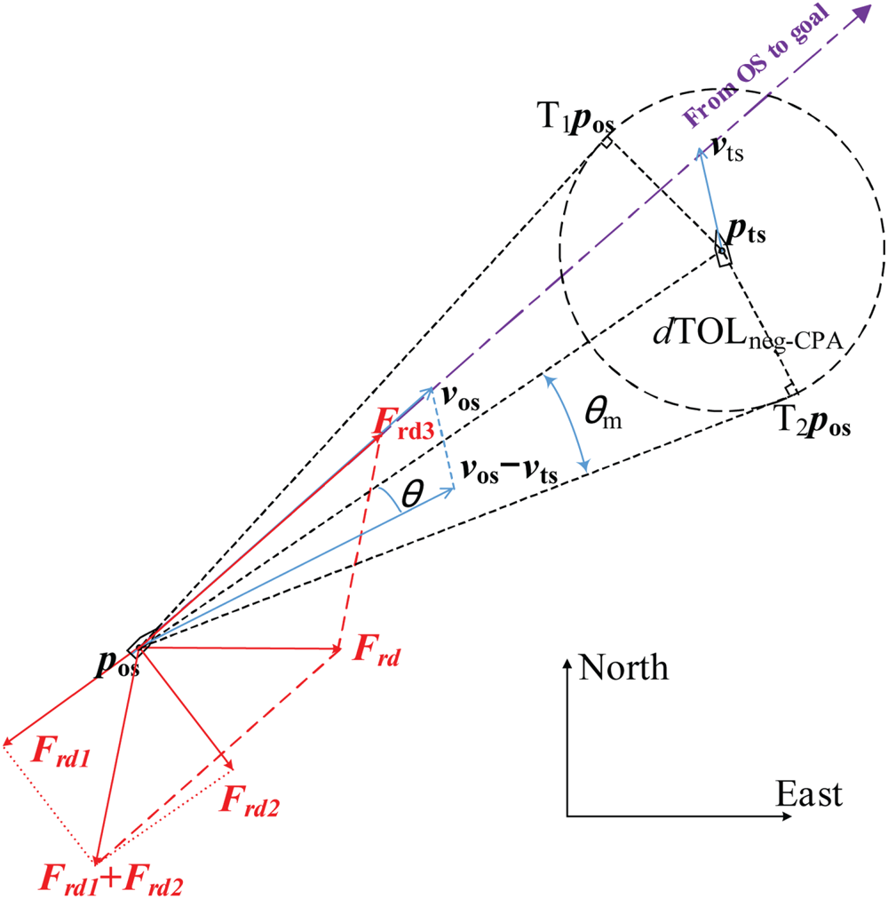
where the direction and significance of each force are shown in Figure 6. The term ${\boldsymbol{n}_{ot}}$ denotes a unit vector pointing to TS or obstacle from own ship (OS); ${d_g}$ is the distance between OS and the goal; d is the distance between OS and TS; ${\theta _\textrm{m}}$ is the angle between any tangent line (T₁p_os or T₂p_os) and the relative position vector ${{\boldsymbol p}_{{\boldsymbol os}}}{{\boldsymbol p}_{{\boldsymbol ts}}}$;$\theta$ is the angle between the relative position vector ${{\boldsymbol p}_{\textrm{ot}}}$(${{\boldsymbol p}_{\textrm{ot}}} = {{\boldsymbol p}_{\textrm{ts}}} - {{\boldsymbol p}_{\textrm{os}}}$) and the relative speed vector ${{\boldsymbol v}_{\textrm{ot}}}$(${{\boldsymbol v}_{\textrm{ot}}} = {{\boldsymbol v}_{\textrm{os}}} - {{\boldsymbol v}_{\textrm{ts}}}$). The risk of collision occurs when the extension line of ${{\boldsymbol v}_{\textrm{os}}}$ crosses the circle of radius $d\textrm{TO}{\textrm{L}_{\textrm{neg - CPA}}}$($\theta < {\theta _\textrm{m}}$); otherwise, the OS can pass through the TS with a safe distance larger than $d\textrm{TO}{\textrm{L}_{\textrm{neg - CPA}}}$. Because the algorithm works on a 2D Cartesian system, we use the Euclidean distance rather than measuring the distance with the haversine formulas.

Figure 6.

Repulsive forces for TS

Terms ${d_{\textrm{emg}}}$ and ${d_{\textrm{neg}}}$ represent the distance criterion of emergency CA and negotiation CA, respectively, $d\textrm{TO}{\textrm{L}_{\textrm{neg - CPA}}}$ and $t\textrm{TO}{\textrm{L}_{\textrm{neg - CPA}}}$ denote the distance and time criteria of negotiation CA, respectively, and $d\textrm{TO}{\textrm{L}_{\textrm{emg - CPA}}}$ and $t\textrm{TO}{\textrm{L}_{\textrm{emg - CPA}}}$ represent the distance and time criteria of emergency CA, respectively. Because all the CA parameters have actual meanings in navigation, and the CA results correspond well to the CA parameters, the modification of the repulsive force model can be comprehended and accepted by navigators.

If there are N TSs, the total repulsive force can be obtained by adding the repulsive forces generated by each TS. The ship will take the corresponding CA actions under the resultant ${F_{sum}}$ for varying conditions and reach the goal. Based on the calculation of attractive and repulsive forces, the total virtual force exerted on the ship can be obtained as:

(24)\begin{equation}{F_{\textrm{sum}}} = {F_{\textrm{att}}} + {F_{\textrm{rep}}}\end{equation}

5.1 EPF modelling for face objects

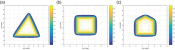
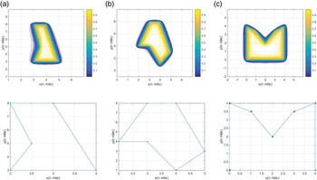
EPF modelling of convex polygons is uncomplicated because the implicit functions of polygons can be obtained using a one-layer intersection operation (${\wedge}$). The potential field at any position generated by the polygons can be obtained as shown in Figure 7.

Figure 7.

Potential fields generated by convex polygons ($\boldsymbol{\alpha}$ = 10 ⋅ 0): (a) triangle, (b) quadrangle, (c) pentagon

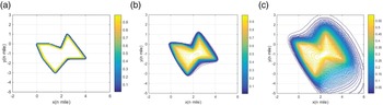
If the polygon includes one or more concave points, the discrete-convex hull method should be applied to obtain its hierarchical structure; the implicit function can then be obtained bottom-up based on the R-function theory. There is only one concave point in Figures 8(a) and 8(b), and the implicit functions of the polygons can be obtained using a two-layer discrete-convex hull calculation, whereas the polygon in Figure 8(c) requires a three-layer discrete-convex hull calculation.

Figure 8.

Potential fields generated by concave polygons ($\boldsymbol{\alpha}$ = 10 ⋅ 0): (a) pentagon, (b)hexagon, (c) heptagon

Figure 9 shows the potential field with different values of $\boldsymbol{\alpha}$. It is obvious that a smaller value of $\boldsymbol{\alpha}$ generates a larger action range of the potential field (the navigable area is smaller around the object). The approach proposed in this study provides an edge-smoothed potential field. The potential field was well-smoothed even around the sharp vertices, which is beneficial for the OA of the MASS.

Figure 9.

Potential fields with different $\alpha$ values: (a) $\boldsymbol{\alpha}$ = 50 ⋅ 0, (b) $\boldsymbol{\alpha}$ = 10 ⋅ 0, (c) $\boldsymbol{\alpha}$ = 1 ⋅ 0

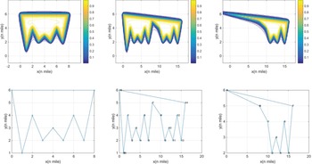
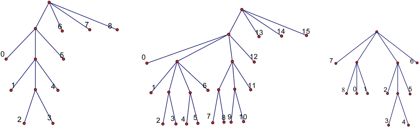
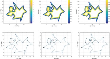
For the polygons shown in Figure 10, their hierarchical structures (as shown in Figure 11) are quite difficult to obtain owing to their complex shapes and concave-convex structures. In current research, automatic potential field modelling of these types of polygons is impractical, while the EPF can be effectively obtained in this study.

Figure 10.

Potential fields of complex polygons ($\boldsymbol{\alpha}$ = 10 ⋅ 0)

Figure 11.

Hierarchical structure of complex polygons

As shown in Figure 12, the hierarchical structure of the polygon becomes more complex when new vertices inserted, the potential field around the inserted points changes accordingly, and the potential field far away remains unchanged. The approach proposed in this study is proven to be feasible and reliable for solving these complicated potential field modelling problems.

Figure 12.

Potential fields of very complex polygons

5.2 EPF modelling based on ENC data

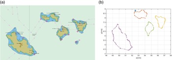
In the vector data provided by the shipboard electronic chart, the 20.0 m isobath data around Zhangzidao (Dalian, China) consist of four islands with 511 sampling points (as shown in Figure 13) (chart number = CN311001, issue date = 2015-08-18, update number = 6, update application date = 2017-12-26, scale = 1:90,000, horizontal geodetic datum = WGS 84). To demonstrate the problem-solving capability of the approach proposed in this study, a series of well-designed tests were conducted using a personal computer with an Intel(R) Xeon(R) CPU E5-1600 v3 @ 3 ⋅ 5 GHz processor, 8 GB RAM, and a 64-bit Windows 10 Professional operating system.

Figure 13.

20 ⋅ 0 m isobath and sampling points near Zhangzidao islands: (a) 20 ⋅ 0 m isobath, (b) sampling points

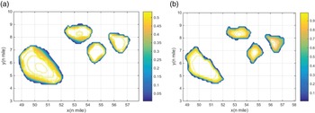
The potential field around Zhangzidao Island was generated based on the 20 ⋅ 0 m isobath data. As shown in Figure 14, a larger value of $\boldsymbol{\alpha}$ results in a larger safe navigation region for the ship, whereas a smaller value of $\boldsymbol{\alpha}$ implies that the ship should maintain a larger distance from the islands. Although a considerable amount of data were provided by the electronic chart, and the shapes of the polygons are extremely complicated, the proposed algorithm could successfully realise the environmental potential field modelling.

Figure 14.

Potential field of 20 ⋅ 0 m depth area: (a) $\boldsymbol{\alpha}$ = 5 ⋅ 0, (b) $\boldsymbol{\alpha}$ = 50 ⋅ 0

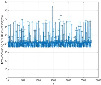
Figure 15 shows the EPF modelling time of the 20 ⋅ 0 m isobath data. The EPF calculation time for each space point is less than 0 ⋅ 1 ms in each iteration. The calculation was relatively time consuming when numerous ENC data were initially imported, because the discrete-convex hull method was applied to obtain the hierarchical structures and the implicit functions based on the R-function theory. Subsequently, the potential field calculation for each point has no direct relationship with the amount and shape of the ENC data. The approach proposed in this study has very small calculations even when operating numerous space data; thus, it can be used in real-time EPF modelling for MASS.

Figure 15.

Time consumption of 1,000 iterations in calculating the EPF for each point

5.3 Path planning in restricted water

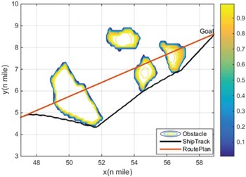
This section presents how one container ship, KangHe, was used as OS to test the OA capability based on the aforementioned 20 ⋅ 0 m isobath data. The CA parameters and initial conditions of the ship are presented in Table 2. $\boldsymbol{\alpha }$ = 50 ⋅ 0 was set for the 20 ⋅ 0 m isobath data. The ship was designed to navigate across three islands successively in accordance with the route plan, and simultaneously detect and maintain a safe distance from obstacles.

Table 2.

Particulars and the initial condition of KangHe

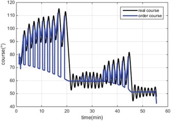
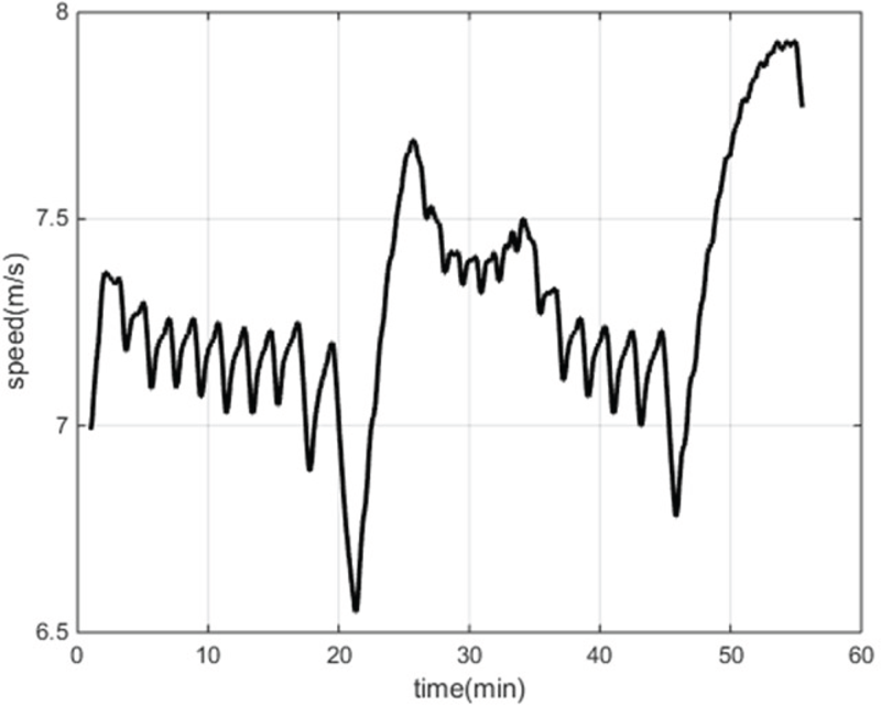
As shown in Figure 16, the OA result shows that KangHe can promptly detect the obstacles and accomplish the OA actions. Figures 17 and 18 show the course and speed changing processes during the test. In the first 20 min, KangHe detected the risk of collision with the first island and altered its course to starboard with a smaller potential field size than the port side. The speed of the ship decreased owing to the frequent operation of the rudder. At 21 min, KangHe headed for the goal with an extra left turn when it had passed the first island, and the speed increased immediately owing to the stable large rudder angle. At 25 min, KangHe started to carry out OA actions to the second and third islands in succession, and the speed of the ship decreased correspondingly owing to the frequent course alteration. At 46 min, KangHe passed and cleared all the islands and altered its course to head for the final destination.

Figure 16.

OA result for KangHe ($\boldsymbol{\alpha}$ = 50 ⋅ 0)

Figure 17.

Course of KangHe in OA test

Figure 18.

Speed of KangHe in OA test

5.4 Path planning in restricted water and with multiple TSs ($\boldsymbol{\alpha}$ = 50 ⋅ 0)

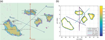
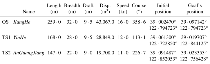
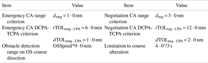
This section presents how the container ship KangHe (OS) was used as a smart ship along with two target container ships, YinHe (TS1) and AnGuangJiang (TS2), to complete the collaborative CA and OA experiment. The initial conditions and ship particulars are presented in Figure 19(a) and Table 3. $\boldsymbol{\alpha}$ = 50 ⋅ 0 was set for the 20 ⋅ 0 m isobath data, and the CA parameters are listed in Table 4.

Figure 19.

Initial conditions of the scenario and collaborative CA results for KangHe: (a) initial scenario conditions, (b) collaborative CA and OA results

Table 3.

Particulars and initial conditions of ships

Table 4.

Parameters for CA tests

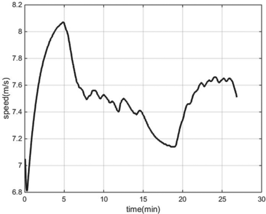
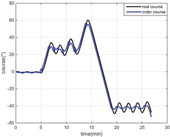
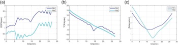
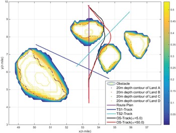
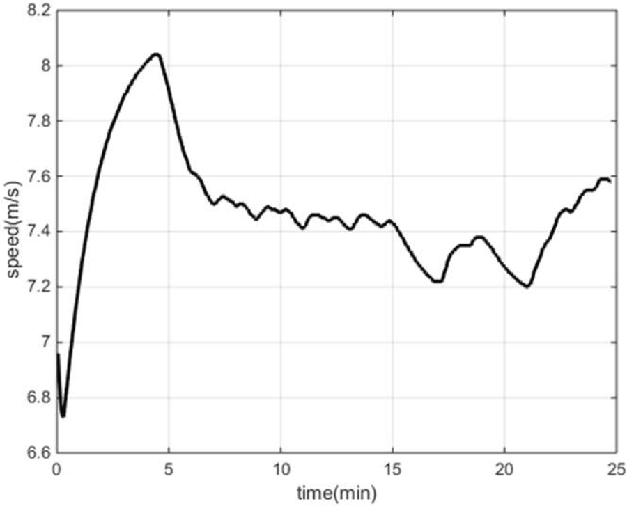
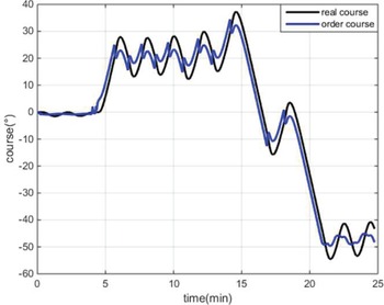
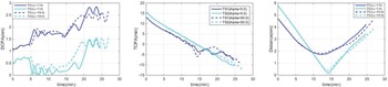
Figure 19(b) shows the collaborative CA and OA results obtained by KangHe. Figures 20 and 21 show the speed and course changing processes, respectively, and Figure 22 shows the DCPAs, TCPAs, and distances during the entire test. By analysing the results and intermediate processes, we observed that the ship navigated on the route plan at full speed in the first 5 min because there was no risk of collision between OS and TSs or obstacles. With the distances between OS and TSs decreasing, the DCPAs and TCPAs decreased accordingly; at 5 min, KangHe started to alter course to starboard as the CA criteria (Negotiation CA TCPA-DCPA and range criterion) with TS1 was fulfilled. At 7 min, the CA criteria with TS2 was fulfilled, KangHe started to carry out CA action with TS1 and TS2, and take OA actions around the islands simultaneously. At 14 min, KangHe started to head for the final destination when it had passed and cleared both TSs and obstacles.

Figure 20.

Speed of KangHe

Figure 21.

Course of KangHe

Figure 22.

DCPAs, TCPAs, and distances between KangHe and TSs: (a) DCPAs, (b) TCPAs, (c) distances

According to the criteria in Table 4, KangHe should maintain a desired DCPA from all vessels and keep a safe distance of 2 ⋅ 0 nm from them. Owing to the restriction of obstacles provided by electronic chart, even though the largest CA actions were applied, KangHe passed and cleared at a distance of 1 ⋅ 81 nm from TS1 and a distance of 0 ⋅ 38 nm from TS2, respectively.

5.5 Path planning in restricted water and with multiple TSs ($\boldsymbol{\alpha}$ = 5 ⋅ 0)

We set $\boldsymbol{\alpha}$ = 5 ⋅ 0 for the 20 ⋅ 0 m isobath data to decrease the navigable area around the islands and conducted the same collaborative CA and OA experiment shown in Section 5.4. Figure 23 shows the CA results for KangHe. Comparisons with the results in Section 5.4 are shown in Figures 23–26. The results show that, in both experiments, the ship conducted the largest CA actions to maintain a relatively safe range of distance from obstacles and other ships.

Figure 23.

Collaborative CA and OA results for KangHe

Figure 24.

Speed of KangHe

Figure 25.

Course of KangHe

Figure 26.

DCPAs, TCPAs, and distances between KangHe and TSs: (a) DCPAs, (b) TCPAs, (c) distances

Through comparison with the results in Section 5.4 (as shown in Figure 26), it can be observed that a smaller value of $\boldsymbol{\alpha}$ induces a larger effective range around the obstacles while reducing the safe navigable region of the ship and restricting the scope of actions. In both experiments, KangHe started to carry out CA action with TS1 at 5 min, and then took CA action with TS1 and TS2 simultaneously. For the restriction of obstacles provided by the electronic chart, KangHe could not pass and clear the TSs at the desired safe distance of 2 ⋅ 0 nm. Because the effective range of the obstacles is larger than that in Section 5.4, the ship needs greater actions to maintain a larger distance from the islands while the action scope in relation to the other ships decreased. Finally, as listed in Table 5, KangHe passed and cleared TS1 and TS2 at distances of 1 ⋅ 72 nm and 0 ⋅ 16 nm, respectively; these distances are smaller than those in Section 5.4.

Table 5.

CA results for KangHe