2. FORMULA FOR LONGITUDE DIFFERENCE IN TERMS OF REDUCED LATITUDE ON A GEODESIC

Geodesic calculations all involve the Clairaut constant or latitude of the vertex along a geodesic, the relationship between the azimuth α and the reduced latitude β can be expressed by the relation (Clairaut, Reference Clairaut1735).

(1)$$c = \cos\beta _V = \cos\beta \,\sin\alpha $$

where e is the first eccentricity, a, b is the semi-major and semi-minor axes, c is the Clairaut constant of a geodesic, β _V is the latitude of vertex along the geodesic, and β is given by the relation shown below:

(2)$$\tan(\beta ) = \sqrt {1 - e^2} \tan (\varphi ),$$

where φ is geodetic latitude.

As mentioned, it is desirable to have a succinct theoretical statement of the solutions to the geodesic, covering all cases in hand before developing these problems' numerical solutions. Referring to Figure 1, it can be seen that the inverse problem is equivalent to solving the geodesic triangle ΔNP ₁P ₂ given two sides and their longitude difference (Δλ). This can be done in more than one way. By using the reduced latitude as the variable of integration such as those presented in Jank and Kivioja (Reference Jank and Kivioja1980) give the longitude and distance integrals as shown in Equations (3) and (4). If the Clairaut constant or latitude of the vertex and one point are given, then the latitude and longitude of any point P of the geodesic are related by Equation (3).

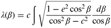(3)$$\lambda (\beta ) = c\int {\sqrt {\displaystyle{{1 - e^2 \cos ^2 \beta} \over {\cos ^2 \beta - c^2}}} \displaystyle{{d\beta} \over {\cos\beta}}} $$

The latitude and distance are related by Equation (4)

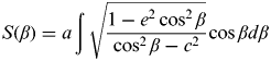(4)$$S(\beta ) = a\int {\sqrt {\displaystyle{{1 - e^2 \cos ^2 \beta} \over {\cos ^2 \beta - c^2}}} \cos\beta d\beta} $$

where the semi-major axis a is 6378137 and eccentricity e is 0·0818191908426215 as adopted in the current WGS-84 ellipsoid model for the Earth.

Figure 1.

Inverse problem of finding the shortest path between two end points.

Applying binomial theorem, Equation (1) and integral techniques expands Equation (3) to the expansion:

(5)$$\lambda (\beta ) = \omega + c\sum\limits_{k = 1}^\infty {C_k ^{1/2} ( - e^2 )^k} \int {\displaystyle{{\cos ^{2k - 1} \beta} \over {\sqrt {\cos ^2 \beta - c^2}}} d\beta} $$

where

$$\omega = \arcsin \left( {\displaystyle{{\tan \beta} \over {\tan \beta _V}}} \right) = \int {\displaystyle{c \over {\sqrt {\cos ^2 \beta - c^2} \cos \,\beta}} d\beta}, \quad{\rm and}\quad\tan \beta _V = \sqrt {1 - c^2 /c}. $$

The vertex latitude β _V is always positive here. Equation (5) gives the longitude formula for the geodesic, and when the eccentricity equals zero, this longitude formula Equation (5) is the same as Napier's rules. Further using the change of variable gives the simplified integral as:

(6)$$\lambda (\beta _1, \beta _2 ) = \omega _{12} + c\sum\limits_{k = 1}^\infty {C_k ^{1/2} ( - e^2 )^k} \int\limits_{\sin \beta _1} ^{\sin \beta _2} {\displaystyle{{(1 - x^2 )^{k - 1}} \over {\sqrt {1 - c^2 - x^2}}}}\, dx$$

where

$$x = \sin \beta, \,\omega _{12} = \arcsin \left( {\displaystyle{{xc} \over {\sqrt {1 - x^2} \sqrt {1 - c^2}}}} \right)\left| \matrix{^{\sin \beta _2} \cr _{\sin \beta _1} } \right.,\quad{\rm and}\quad- \beta _V \leqslant \beta \leqslant \beta _V. $$

By applying the binomial theorem again this expands the numerator in the right-hand side integrand of Equation (6) and this result can be exactly integrated as the following:

(7)$$\lambda (\beta _1, \beta _2 ) = \omega _{12} + c \cdot \sum\limits_{k = 1}^\infty {(M_{k,1} \cdot {\rm}} \sigma + M_{k,2} \cdot \mu )e^{2k} \left| \matrix{^{\sin \beta _2} \cr _{\sin \beta _1} } \right.$$

where $u = \sqrt {1 - c^2  - x^2} $ and 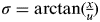$\sigma = \arctan ({\textstyle{x \over u}})$.

The expansion of Equation (6) can be conveniently integrated to arbitrarily order by CAS such as Maple® etc. which yields the two coefficient matrices by truncating the expansion at order e ¹⁰ up to M ₄, as shown below:

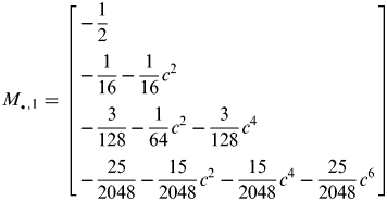(8)$$M_{_ \bullet, 1} = \left[ \matrix{ - \displaystyle{1 \over 2} \cr - \displaystyle{1 \over {16}} - \displaystyle{1 \over {16}}c^2 \cr - \displaystyle{3 \over {128}} - \displaystyle{1 \over {64}}c^2 - \displaystyle{3 \over {128}}c^4 \cr - \displaystyle{{25} \over {2048}} - \displaystyle{{15} \over {2048}}c^2 - \displaystyle{{15} \over {2048}}c^4 - \displaystyle{{25} \over {2048}}c^6 } \right]$$

and

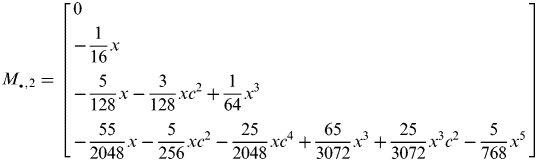(9)$$M_{_ \bullet, 2} =\left[ \matrix{0 \cr - \displaystyle{1 \over {16}}x \cr - \displaystyle{5 \over {128}}x - \displaystyle{3 \over {128}}xc^2 + \displaystyle{1 \over {64}}x^3 \cr - \displaystyle{{55} \over {2048}}x - \displaystyle{5 \over {256}}xc^2 - \displaystyle{{25} \over {2048}}xc^4 + \displaystyle{{65} \over {3072}}x^3 + \displaystyle{{25} \over {3072}}x^3 c^2 - \displaystyle{5 \over {768}}x^5 } \right]$$

where M _•,i=[M _1,i … M _4,i ]^T and i=1, 2.

The latitudes between interval [−β _V, β _V] cannot sketch all the geodesic segments of arbitrary length, so to overcome this disadvantage, one must introduce another variable t with interval [−∞ ∞] and also imply the following properties of Equation (10) which is related to latitudes.

(10)$$\beta (t) = ( - 1)^p {\rm \Delta} t + ( - 1)^{\,p + 1} \beta _V $$

where p=FIX (t+β _V, 2β _V) is the number of phase (2β _V) [FIX(..) rounds the element of (..) to the nearest integer] and Δt=REM (t+β _V, 2β _V) is the fraction of variable t in regard to the phase (REM computes the remainder after division).

As the relationship between variables t and latitude is many-to-one, Equation (10) is a periodical function that oscillates between two opposite vertices as shown in Figure 2.

Figure 2.

The relationship of the oscillating reduced latitude between two vertices and variable t. Two different conditional integrals depend on the phase number.

The integral must be transformed into the following conditional function modified to accommodate variable t. But because although the range of variable t is [−∞ ∞], when integrating Equation (7) it will only give one corresponding value in the range of [−β _V, β_V], thus to solve this problem, one must first determine how many phases (β _V) does the variable t have in regard to Equation (7). If even phases, then use the conditional function Equation (11) (top left rectangle in Figure 2), whereas if it equals odd phases, then use the other conditional (bottom left rectangle in Figure 2).

$$\lambda (0,t) = 2p\Delta \lambda _V + \lambda (0,( - 1)^p \beta (t))$$

i.e.

(11)$$\lambda (0,t) = \left\{ \matrix{2p{\rm \Delta} \lambda _V + \lambda (0,\beta (t)),\quad p \in 2n \cr 2p{\rm \Delta} \lambda _V + \lambda (\beta (t),0),\quad p \in 2n + 1 } \right.$$

where the longitude difference Δλ _V=λ(0, β _V) of one phase equals one quarter cycle wrapping the Equator and the latitude β(t) defined in Equation (10).

Again when variable t is applied to Equation (1), it will only give one corresponding value in the range of [−βv βv]. We solve this problem by first determining how many phases (2β _V) does variable t have in regard to 2β _V. If the phases of variable t are even phases, then use the first condition of Equation (12) (top right rectangle in Figure 2), whereas then otherwise use the second condition of Equation (12) (bottom right rectangle in Figure 2), using Equation (1) gives the course function below on waypoints along the geodesic.

$$\alpha (t) = \pm \left[ {MOD(\,p,2) {\cdot} \pi + ( - 1)^p \sin ^{ - 1} (\cos \beta _V /\cos \beta (t))} \right]$$

i.e.

(12)$$\alpha (t) = \pm \left\{ \matrix{\sin ^{ - 1} (\cos \beta _V /\cos \beta (t)),& p = 2n \cr \pi - \sin ^{ - 1} (\cos \beta _V /\cos \beta (t)),&p = 2n + 1 } \right.$$

If the geodesic is westbound, the positive sign (+) is adopted, otherwise the negative sign (−) is adopted.

The two conditions of Equation (12) mean that the courses are northeast bound or southeast bound as shown in Figure 2, because the default travel direction in the canonical configurations is eastbound.

Apply Equation (11) to calculate the longitudes of the path departing from the first node to the fifth node (passing 2 cycles) where t has the interval [0°, 720°].

Figure 3 shows the oscillations of a geodesic on the spheroid and a great circle on the sphere. Point F on the geodesic crosses the Equator at longitude 0, heading in a northeast direction reaching a maximum northern latitude, then descends in a southeast direction crossing the Equator at a certain longitude, reaching a maximum southern latitude, then ascends in a north-eastern direction crossing the Equator again at point F1 (the red line). This is one cycle of the geodesic, but the longitude difference of the end of one cycle does not equal 360° due to the eccentricity of the spheroid and is not a closed curve, hence the geodesic does not repeat after a complete cycle, unlike its great circle counterpart which repeats after a complete cycle at point F2 (the brown line).

Figure 3.

The oscillation of a geodesic on a spheroid. Note: The eccentricity has been increased to 0·5 in order to accentuate the spheroidal effects.

The geodesic curve will lag a certain longitude compared to a great circle after a complete cycle. Therefore after passing many circuits, it will wrap a band on the spheroid between two opposite vertices shown in Figure 4.

Figure 4.

A geodesic curve wraps a band on a spheroid after many circuits.

Applying Equation (11) gives the longitude difference between the south and north vertices:

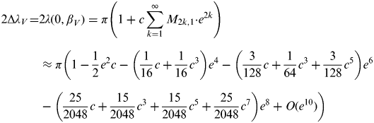(13)$$\eqalign{2{\rm \Delta} \lambda _V\! = & 2\lambda (0,\beta _V ) = \pi \left(1 + c\sum\limits_{k = 1}^\infty {M_{2k,1} {\cdot} {\rm}} e^{2k} \right) \cr & \approx \pi \bigg(1 - \displaystyle{1 \over 2}e^2 c - \left( {\displaystyle{1 \over {16}}c + \displaystyle{1 \over {16}}c^3} \right)e^4 - \left( {\displaystyle{3 \over {128}}c + \displaystyle{1 \over {64}}c^3 + \displaystyle{3 \over {128}}c^5} \right)e^6 \cr & - \left( {\displaystyle{{25} \over {2048}}c + \displaystyle{{15} \over {2048}}c^3 + \displaystyle{{15} \over {2048}}c^5 + \displaystyle{{25} \over {2048}}c^7} \right)e^8 + O(e^{10} )\bigg)} $$

where $x = \sin (\beta _V ) = \sqrt {1 - c^2} $.

The nearly antipodal regions are located within the interval [Δλ _V, π]; there are two geodesics mirrored in the Equator and with complementary azimuths at each point (Figure 5). As stated before, in the special case when the given points are located at the poles of the spheroid, all meridians are geodesics (Sjöberg, Reference Sjöberg2012).

Figure 5.

The variation of geodesic as a function of Clairaut constant c for starting point β ₁=−30°. Note: the eccentricity exaggeratedly is set to 0·5.

The track of the two mirrored geodesics for various starting latitudes can be described by the definition of variable t shown below:

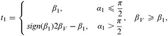(14)$$t_1 = \left\{ {\matrix{ {\beta _1,} & {\alpha _1 \leqslant \displaystyle{\pi \over 2}} \cr {sign(\beta _1 )2\beta _V - \beta _1,} & {\alpha _1 \gt \displaystyle{\pi \over 2}} \cr},} \right.\quad \beta _V \geqslant \beta _1, $$

and the longitudes and latitudes can be obtained by Equation (15):

(15)$${\rm \Delta} \lambda = \lambda (t) - \lambda (t_1 ),\quad t = \left[ {t_1, t_1 + 2\beta _V} \right]$$

Using Equation (13) gives the nearly antipodal regions for various vertices shown in Figure 6.

Figure 6.

Nearly antipodal regions at various vertices.

Figure 6 shows that the longitude difference between the two opposite vertices depends on the vertex. It equals π only when the constant c=0 and is slightly shorter than π. The geodesic is not closed around the spheroid for c≠0, and its period is somewhat shorter than 2π. Applying integration by parts gives a different integral for Equation (3):

(16)$$\lambda (\beta ) = \omega \sqrt {1 - e^2 \cos ^2 \beta} - \int {\omega \displaystyle{{e^2 \sin \beta \cos \beta} \over {\sqrt {1 - e^2 \cos ^2 \beta}}} d\beta} $$

The longitude difference between the two opposite vertices has a minimum value when c equals one. As the latitude of the vertex approaches to zero, the LHS of integral Equation (16) vanishes. The exact formula of the longitude difference between two opposite vertices can be given or setting c=1 in Equation (13) also gives the approximate series Equation (17).

(17)$$\eqalign{2\Delta \lambda _V = \lambda (\beta _1 = 0,\beta _2 \to 0,1) = \pi \sqrt {1 - e^2} \approx \pi \left( {1 - \displaystyle{1 \over 2}e^2 - \displaystyle{1 \over 8}e^4 \displaystyle{1 \over {16}}e^6 - \displaystyle{5 \over {128}}e^8 - \ldots} \right)}$$

The binominal series of the second last term of Equation (17) with respect to e ² is approximately the last term of the above. This is the so-called “lift-off longitude” (Rapp, Reference Rapp1993). The antipodal region (Schmidt, Reference Schmidt2006) is located roughly within 36′.2 from the antipode at the Equator adopting the WGS-84 Earth datum.

3. ARC LENGTH IN TERMS OF REDUCED LATITUDE ON A GEODESIC

Geodesic distances are very important as they are the shortest distances. Applying the binomial theorem, Equation (1), and integral techniques expands Equation (4) to the series Equation (18):

(18)$$S(\beta ) = a \cdot \sigma + a\sum\limits_{k = 1}^\infty {C_k^{1/2} ( - e^2 )^k \int {\displaystyle{{\cos ^{2k + 1} \beta} \over {\sqrt {\cos ^2 \beta - c^2}}} d\beta}} $$

where

$$\sigma = \arctan \left( {\displaystyle{{\sin\beta} \over {\sqrt {\cos ^2 \beta - c^2}}}} \right) = \int {\displaystyle{{\cos \beta} \over {\sqrt {\cos ^2 \beta - c^2}}} d\beta.} $$

Setting x=sin β, thus using the change of variable transforms Equation (18) to Equation (19).

(19)$$S(\beta _1, \beta _2 ) = a \cdot \sigma + a\sum\limits_{k = 1}^\infty {C_k^{1/2} ( - e^2 )^k \int\limits_{\sin \beta _1} ^{\sin \beta _1} {\displaystyle{{(1 - x^2 )^k} \over {\sqrt {1 - c^2 - x^2}}}}}\, dx$$

Again, by using the binomial theorem, the numerator in the right-hand side integrand of Equation (19) may be expanded, and this result can be exactly integrated as Equation (20):

(20)$$S(\beta _1, \beta _2 ) = a \cdot \sigma + a\sum\limits_{k = 1}^\infty {(N_{k,1} \cdot \sigma + N_{k,2} \cdot {\rm}} \mu )e^{2k} \left| \matrix{^{\sin \beta _2} \cr _{\sin \beta _1} } \right.$$

where $u = \sqrt {1 - c^2  - x^2} $ and 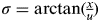$\sigma = \arctan ({\textstyle{x \over u}})$, and β _V ⩽ β ⩽−β _V.

Integrating Equation (19) in terms of CAS or handwork gives the two matrixes of coefficients by truncating the expansion at order e ¹⁰ and N ₅ up to e ⁸ and N ₄.

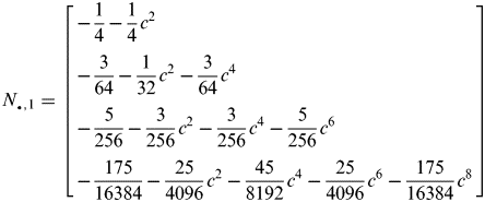(21)$$N_{_ \bullet, 1}=\left[ \matrix{ - \displaystyle{1 \over 4} - \displaystyle{1 \over 4}c^2 \cr - \displaystyle{3 \over {64}} - \displaystyle{1 \over {32}}c^2 - \displaystyle{3 \over {64}}c^4 \cr - \displaystyle{5 \over {256}} - \displaystyle{3 \over {256}}c^2 - \displaystyle{3 \over {256}}c^4 -\displaystyle{5 \over {256}}c^6 \cr - \displaystyle{{175} \over {16384}} - \displaystyle{{25} \over {4096}}c^2 - \displaystyle{{45} \over {8192}}c^4 - \displaystyle{{25} \over {4096}}c^6 - \displaystyle{{175} \over {16384}}c^8 } \right]$$

and

(22)$$N_{_ \bullet, 2} =\left[ \matrix{ - \displaystyle{1 \over 4}x \cr - \displaystyle{5 \over {64}}x - \displaystyle{3 \over {64}}xc^2 + \displaystyle{1 \over {32}}x^3 \cr - \displaystyle{{11} \over {256}}x - \displaystyle{1 \over {32}}xc^2 - \displaystyle{5 \over {256}}xc^4 + \displaystyle{{13} \over {384}}x^3 + \displaystyle{5 \over {384}}x^3 c^2 - \displaystyle{1 \over {96}}x^5 \cr \left( \matrix{ - \displaystyle{{465} \over {16384}}x - \displaystyle{{365} \over {16384}}xc^2 - \displaystyle{{275} \over {16384}}xc^4 - \displaystyle{{175} \over {16384}}xc^6 + \displaystyle{{815} \over {24576}}x^3 + {\rm \ldots} \cr \displaystyle{{75} \over {4096}}x^3 c^2 + \displaystyle{{175} \over {24576}}x^3 c^4 - \displaystyle{{125} \over {6144}}x^5 - \displaystyle{{35} \over {6144}}x^5 c^2 + \displaystyle{5 \over {1024}}x^7 } \right) } \right]$$

where N _•,i=[N _1,i … N _4,i ]^T and i=1, 2.

Again, since the latitudes between the interval [−β _Vβ_V] cannot sketch all the geodesic segments of arbitrarily length, one must introduce the variable t as presented in Equation (10). The integral Equation (20) must be transformed into the following conditional function modified to accommodate variable t.

(23)$$S(0,t) = 2p{\rm \Delta} S_V + S(0,( - 1)^p \beta (t))$$

where ΔS _V=S(0, β _V) is the distance from node to vertex as Equation (24) and the p as defined by Equation (11).

(24)$$\eqalign{\Delta S_V = & S(0,\beta _V ) \cr = & \displaystyle{a \over 2}\pi \left( {1 + \sum\limits_{k = 1}^\infty {N_{2i,1}} \cdot e^{2k}} \right)\! \approx a\pi \left( {1\! -\!\! \left( {\displaystyle{1 \over 4} + \displaystyle{1 \over 4}c^2} \right)}\! \right)e^2\! -\! \left( {\displaystyle{3 \over {64}} + \displaystyle{1 \over {32}}c^2 + \displaystyle{3 \over {64}}c^4} \right)e^4 \ldots} $$

The arc length of a geodesic is the meridian when the vertex is at the pole(s). This shows that the arc length between the two opposite vertices or two nodes depends on the Clairaut constant, and it shall equal the meridional distance when the constant c=0. Applying integration by parts gives a different integral Equation (25) for Equation (3).

(25)$$S(\beta ) = a\sigma \sqrt {1 - e^2 \cos \beta} - a\int {\sigma \displaystyle{{e^2 \sin \beta \cos \beta} \over {\sqrt {1 - e^2 \cos ^2 \beta}}} d\beta} $$

The geodesic arc length between the two opposite vertices has a minimum value when c=1. As before, as the latitude of vertex approaches zero, the LSH integral of Equation (25) vanishes, thus the exact formula of the curve length can be given or the setting c=1 of Equation (24) gives the series approximately.

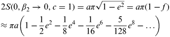(26)$$\eqalign{& 2S(0,\beta _2 \to 0,c = 1) = a\pi \sqrt {1 - e^2} = a\pi (1 - f) \cr &\!\! \approx \pi a\left( {1 - \displaystyle{1 \over 2}e^2 - \displaystyle{1 \over 8}e^4 - \displaystyle{1 \over {16}}e^6 - \displaystyle{5 \over {128}}e^8 - \ldots} \right)} $$

In the case of when c=1, the geodesic runs along the equator, Equation (26) is consistent with Equation (17). Applying Equations (17) or (26) gives the solution of antipodal region at the Equator.

(27)$$\varepsilon = \pi \left( {1 - \sqrt {1 - e^2}} \right) = \pi f.$$

We apply the parameters according to WGS 84 to obtain the maximum distance aε=67·18197165 km along the geodesic on the Equator which is less than one half circle of the Equator. The great ellipse or the normal section passing antipodes located on the Equator cannot be determined, so the track along the Equator may be chosen for convenience. This means that the maximum distance difference between a geodesic and a great ellipse (or normal section) is the distance of one half circle of the Equator minus the length of one half elliptic arc length of the meridian as shown in Equation (28).

(28)$$\eqalign{a\pi - 2S(0,\pi /2,c = 0) = &\, 20037508 {\cdot} 343 - 20003931 {\cdot} 435 \cr = & - 33576 {\cdot} 908\;{\rm m} = 18 {\cdot} 1300799\;{\rm nautical}\;{\rm miles}.} $$

In our previous work (Tseng et al., Reference Tseng, Guo and Liu2013), the maximum error for a longitude difference of 90° from the Equator to a certain latitude is about 7 metres at approximately 45° latitude. The results mean that nearly antipodal points at lower latitudes will generate bigger errors between the great ellipse and geodesic.

4. INVERSE PROBLEM OF GEODESIC SAILING

The inverse problem is intrinsically more complicated than the direct problem because the given longitude λ ₁₂ is related to the corresponding unknown equatorial azimuth α ₀ or latitude β _V of the geodesic vertex. Thus, the inverse problem inevitably becomes a root-finding exercise. This problem can be tackled as follows.

Assume that β _V is known. Solve the hybrid geodesic problem: given β ₁, β ₂, and β _V, find the calculated λ ₁₂ corresponding to the first intersection of the geodesic with the parallel of latitude β ₂ which is the resulting longitude difference of given initial λ ₁₂ in general cases; so adjust β _V using Newton's method, secant method, or other root-finding methods until the correct λ ₁₂ is obtained. The two endpoints can be put in a canonical configuration,

(29)$$\beta _1 \leqslant 0,\quad\beta _1 \leqslant \beta _2 \leqslant - \beta _1,\quad 0 \leqslant \beta _{12} \leqslant \pi. $$

This may be accomplished by swapping the end points and the signs of the coordinates if necessary, and the solution may similarly be transformed to apply to the original points. All geodesics with β _V=[|β ₁|, π/2] and α ₁=[0, π] intersect the parallel of latitude β ₂ with λ ₁₂₌[0, π]. Meridional (λ ₁₂=0 or π) and equatorial (β ₁=β ₂=0, and λ ₁₂<=(1− f)π) geodesics are treated as special cases. The general case is solved by the analog of Newton's method as outlined below. The longitude difference of a geodesic depends on its initial azimuth as northeast or southeast shown as the conditional Equation (30) that is constrained by Condition (29). If the course is southeast bound, then the reference initial point is near the destination and the geodesic passes the vertex and the variable t ₁ is set to −2β _V−β ₁). Otherwise, the geodesic does not pass the vertex; the variable t ₁ is set to β ₁.

(30)$$\lambda (t_1, t_2 ),\quad t_2 = \beta _2,\quad t_1 = - 2NS {\cdot} \beta _V + ( - 1)^{NS} \beta _1 $$

where the direction logical variable NS is given in Equation (32).

The geodesic with vertex latitude β ₁ departing from latitude β ₁ intersects the parallel of the latitude β ₂ at the longitude difference λ _NS as shown in Equation (31):

(31)$$\lambda _{NS} = \lambda (\beta _1, \beta _2, c = \cos (\beta _1 ))$$

The following conditions give the azimuth of a geodesic. If longitude difference λ ₁₂ is greater than the longitude difference λ _NS of the intersection, the initial course of the geodesic is southeast bound, otherwise it is northeast bound as shown in Figure 5. The logical variable NS is decided by Equation (32):

(32)$$NS = \left\{ \matrix{1,(\lambda _{12} - {\rm \Delta} \lambda _{NS} ) \gt 0 \cr 0,(\lambda _{12} - {\rm \Delta} \lambda _{NS} ) \lt 0 } \right.$$

Vincenty (Reference Vincenty1975a) used the iterative method of Helmert (Reference Helmert1880) to solve the inverse problem and was aware of its failure to converge for nearly antipodal regions. In an unpublished report (Vincenty, Reference Vincenty1975b) gives a modification of his method which deals with this case. Unfortunately, this method sometimes requires many thousands of iterations to converge, whereas the approach shown below is used to approximate Newton's method and the innovative iterative method proposed here for nearly antipodal regions only requires a few iterations.

Karney (Reference Karney2013) uses Newton's method, requires a good starting guess and uses more complex procedures which even involves firstly calculating the reduced length of the geodesic and solving a fourth-order polynomial merely to find a good starting point, and may involve a high computational cost. Using Newton's Method solves the inverse problem by the derivative of longitude difference with respect to c or β _V as shown:

(33)$$c = c - \displaystyle{{\lambda (t_1, t_2 ) - \lambda _{12}} \over {\displaystyle{{\partial \lambda (t_1, t_2 )} \over {\partial c}}}},\quad\beta _V = \beta _V - \displaystyle{{\lambda (t_1, t_2, c = \cos (\beta _V )) - \lambda _{12}} \over {\displaystyle{{\partial \lambda (t_1, t_2 )} \over {\partial \beta _V}}}} $$

Differentiating the longitude difference function with respect to c gives

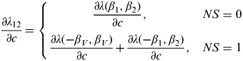(34)$$\displaystyle{{\partial \lambda _{12}} \over {\partial c}} = \left\{ {\matrix{ {\displaystyle{{\partial \lambda (\beta _1, \beta _2 )} \over {\partial c}},} & {NS = 0} \cr {\displaystyle{{\partial \lambda ( - \beta _V, \beta _V )} \over {\partial c}} + \displaystyle{{\partial \lambda ( - \beta _1, \beta _2 )} \over {\partial c}},} & {NS = 1} \cr}} \right.$$

where the derivative of the function with respect to c in-between the two opposite vertices is

(35)$$\displaystyle{{\partial \lambda (\beta \hskip1pt\prime _{\hskip-3pt 1}, \beta \hskip1pt\prime _{\hskip-3pt 2} )} \over {\partial c}} = \int_{\beta \hskip1pt\prime _{\hskip-3pt 1}} ^{\beta \hskip1pt\prime _{\hskip-3pt 2}} {\left( {\displaystyle{{\sqrt {1 - e^2 \cos ^2} \beta} \over {\sqrt {\cos ^2 \beta - c^2} \cos \beta}} + \displaystyle{{c^2 \sqrt {1 - e^2 \cos ^2 \beta}} \over {(\cos ^2 \beta - c^2 )^{3/2} \cos \beta}}} \right)d\beta} $$

If the segment of the geodesic passes the vertex, the derivative of longitude difference function with respect to c or β _V involves the segment of geodesic from the south vertex to the north vertex, which is non-differentiable as shown below.

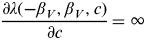(36)$$\displaystyle{{\partial \lambda ( - \beta _V, \beta _V, c)} \over {\partial c}} = \infty $$

By using the finite difference method, the derivative can be completely replaced in all situations to avoid the non-differentiable condition as the following Equation (37).

(37)$$\displaystyle{{\partial \lambda} \over {\partial \beta _V}} \cong \displaystyle{{\Delta _h [\lambda ](\beta _V )} \over h} = _{h \to 0}^{\lim} \displaystyle{{\lambda (\beta _V + h) - \lambda (\beta _V )} \over h}$$

In the general case, the Clairaut constant and the reduced latitude of the vertex can be represented in terms of longitude difference and latitudes of the two given endpoints.

The starting point for Newton's method can be approximately obtained by the spherical model. In rectangular coordinates, any point on the unitary sphere can be represented as coordinates of

(38)$${\mathop{P}\limits^{\rightharpoonup}} = (\cos\beta \,\cos\omega, \cos\beta \,\sin\omega, \sin\beta )$$

where ω can be replaced with λ approximately for the first iteration.

The normal to the plane of a great circle is the cross product of the two vectors as shown:

(39)$${\mathop{N}\limits^{\rightharpoonup}} = [x_N\ y_N\ z_N ] = {\mathop{P}\limits^{\rightharpoonup}} _1 {\rm \times} {\mathop{P}\limits^{\rightharpoonup}} _2 $$

The latitude of the vertex equals to the angle between the Z-axis and the normal to the plane spanned by the two vectors.

(40)$$\tan \beta _V = \sqrt {x_N^2 + y_N^2} /z_N $$

Using the algebra symbolic system and the trigonometric identities expands the last expression as Equation (41)). Sjöberg (Reference Sjöberg2007; Reference Sjöberg2012) has also proven Equation (41) by spherical trigonometric methods.

(41)$$\tan \beta _V = \sqrt {\tan ^2 \beta _1 + \tan ^2 \beta _2 - 2\tan \beta _1 \tan \beta _2 \cos \lambda _{12} /\sin \lambda _{12}} $$

Using trigonometric identity rewrites the formula for the Clairaut constant c as Equation (42).

(42)$$c = \cos \beta _V = \sin \lambda _{12} /\sqrt {\tan ^2 \beta _1 + \tan ^2 \beta _2 - 2\tan \beta _1 \tan \beta _2 \cos \lambda _{12} + \sin \lambda _{12}} $$

If the two endpoints are located on the equator (β ₁=β ₂=0), then by applying Equations (13) and (17), the various cases for the Clairaut constant c can be determined by the following conditional Equation (43):

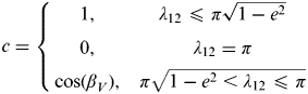(43)$$c = \left\{ {\matrix{ 1, & {\lambda _{12} \leqslant \pi \sqrt {1 - e^2}} \cr 0, & {\lambda _{12} = \pi} \cr {\cos (\beta _V )}, & {\pi \sqrt {1 - e^2 \lt \lambda _{12} \leqslant \pi}} \cr}} \right.$$

If the two endpoints are located in the nearly antipodal regions (β ₁+β ₂=0) and 2Δλ _V<λ ₁₂), then applying Equations (13) and (17), the various cases for the Clairaut constant c can be determined by the following conditional Equation (44):

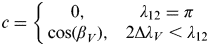(44)$$c = \left\{ {\matrix{ 0, & {\lambda _{12} = \pi} \cr {\cos (\beta _V ),} & {2\Delta \lambda _V \lt \lambda _{12}} \cr}} \right.$$

where the vertex reduced latitude (β _V) is subject to Equation (13) as the following repetitively:

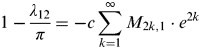(45)$$1 - \displaystyle{{\lambda _{12}} \over \pi} = - c\sum\limits_{k = 1}^\infty {M_{2k,1} \cdot e^{2k}} $$

Truncating the series toward the first order gives the approximate Clairaut constant c as shown in Equation (46):

(46)$$c_k = \displaystyle{{2(\pi - \lambda _{12} )} \over {e^2 \pi}} $$

The accurate value can be re-approached several times by the following iterative computation Equation (47) or Newton's method:

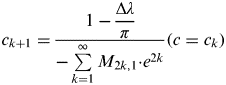(47)$$c_{k + 1} = \displaystyle{{1 - \displaystyle{{{\rm \Delta} \lambda} \over \pi}} \over { - \sum\limits_{k = 1}^\infty {M_{2k,1} {\cdot} e^{2k}}}} (c = c_k )$$

Equation (47) shows that the solution to the Clairaut constant has unique values for the two ends in the nearly antipodal regions.

Applying the method of the asteroid plane provided by Karney (Reference Karney2013) can accelerate the speed of convergence. But the faster method implies a higher computational cost to solve the quartic equation before starting the iteration. Once the Clairaut constant and the coordinates of the end points of the geodesic are known, the azimuths of the geodesic at the end points may be determined from Equation (48)

(48)$$\alpha _1 = NS {\cdot} \pi + ( - 1)^{NS} \sin ^{ - 1} (\cos \beta _V /\cos \beta _1 )$$

and

(49)$$ {{\rm \alpha} _2 = \cos \beta _V /\cos \beta _2} $$

Procedures for solving the geodesic inverse problem are summarised in Figure 7, which gives all the required algorithms clearly for the readers' convenience.

Figure 7.

The flow chart of algorithm for solving the geodesic inverse problem.

* eps and h is very small value; it is set to the value 10−10 here.

5. NUMERICAL RESULTS FOR DISTANCE AND LONGITUDE EQUATIONS

Three examples are represented in this section. The first two samples are cited from Tables 4 and 5 of Karney (Reference Karney2013). Those data obtained from his results are compared with the results computed by the methods proposed here, which are also compared with the results obtained from the great ellipse (GE) provided in our previous work (Tseng et al., Reference Tseng, Guo, Liu and Wu2012a). Analysis of the efficiency and accuracy between such comparisons are shown in Tables 2 and 3. It can be seen that the innovative iterative method proposed here for nearly antipodal regions or general cases only requires a few iterations.

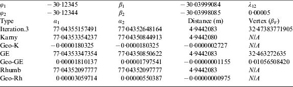
The first example is specified by φ ₁=−30·12345°, φ ₂=−30·12344°, and λ ₁₂=0·00005° as shown in Figure 8 (left). Because the two points are not nearly antipodal, an initial guess for the reduced latitude β _V of the vertex is found from Equation (41). However, in cases of when two points are very close to each other, the line is short enough that the error in β _V is negligible; the solution of this inverse problem is completed by using finite difference or Newton's method as shown in Table 1.

Figure 8.

The track (left) of geodesic between very closely points. The tracks (right) of geodesic and great ellipse from two nearly antipodal points.

Table 1.

Comparing the results of calculations with two very close endpoints.

Note: Geo-K=differences between the result calculated here and Karney's result

As the two points are very close to each other, the line is very short and the differences between the geodesic and GE are very small; both sailing methods may be applied here, even using rhumbline or plane sailing (Tseng et al., Reference Tseng, Earle and Guo2012b) gives near identical results (shown in Table 1).

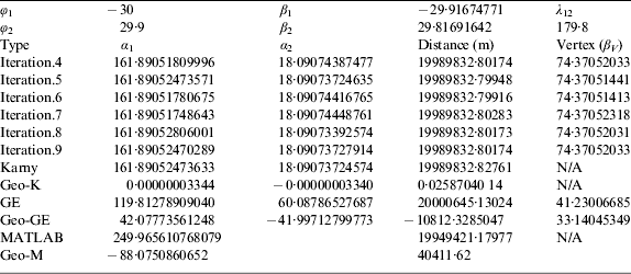
A second example is specified by φ ₁=−30°, φ ₂=29·9°, and λ ₁₂=179·8° in Figure 8 (right). In this case, the points are nearly antipodal, an initial guess for the Clairaut constant c is found by solving Equation (46), then the solution of this problem is completed by using finite difference or Newton's method, the result is shown in Table 2.

Table 2.

Comparing the results of calculations for Example 2.

The function [dist,az]=distance(lat1,lon1,lat2,lon2,ellipsoid) provided in the Mapping Toolbox^® by MATLAB^® computes the geodesic distance and azimuth assuming that the points lie on the reference ellipsoid defined by the input ellipsoid. This distance function of MATLAB adopts Vincenty's algorithm which sometimes requires many thousands of iterations or converges to a wrong answer in nearly antipodal regions, whereas the approximated Newton's method and innovative iterative method for nearly antipodal regions as described here only requires a few iterations. As shown in Table 2, Karney (Reference Karney2013) uses much more complex procedures which even involve calculating the reduced length of the geodesic and solving a fourth-order polynomial to merely find a good starting point for his method.

In the case of closely near antipodal regions, using the MATLAB^® distance function for this problem gives the incorrect result; the initial course and distance have huge errors and cannot be accepted. The discrepancies between the results computed by the proposed methods described here and of those provided by Karney (Reference Karney2013) are negligible; the distance difference between the two is approximately 2·5 cm for this very long geodesic. These results show that the new methods proposed here can be accepted in practical sailing and geodesic calculations. The discrepancies have arisen from truncating the expansion of Equations (7) and (10) both at order e ¹⁰ leaving the series up to e ⁸, the truncated series generates errors in ae ⁸ order which are centimetre-level.

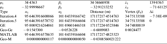
As shown in Table 3, the GE distance is 10812·32 m (5·9 nautical miles) further than the distance of geodesic with the same input values. Fortunately in most cases of navigation, the endpoints of practical sailing are seldom located closely in nearly antipodal regions.

Table 3.

Determining route from Yokohama to Valparaiso.

The third numerical example presented has a very long navigational route with longitude differences between two endpoints of about 145°. The route is from Valparaiso-Chile (32° 59·998′S, 71° 36·675′W) to Yokohama-Japan (34° 26·178′ N, 139° 51·39 E).

The results of Example 3 are shown in Table 3. The geodesic is slightly more curved than the great ellipse (see Figure 9). The eccentricity is exaggerated and set to 0·5 to show the difference between the GE and geodesic. In this example the discrepancy between the two distances (GE: 9242·561583 nautical miles, geodesic: 9242·558019 nautical miles) is approximately 6·6 metres, for which the GE can be accepted for the practical purposes of navigation. As the track doesn't pass through the vertex, the differences of the two tracks are very small which can be negligible in practice. Also, the geodesic distance obtained from the truncated series provided here generates tiny discrepancies compared to those obtained from the different truncated series terms of the in-built function “geodesicinv.m” in MATLAB™; both generate near consistent results.

Figure 9.

The track from Yokohama, Japan to Valparaiso, Chile.

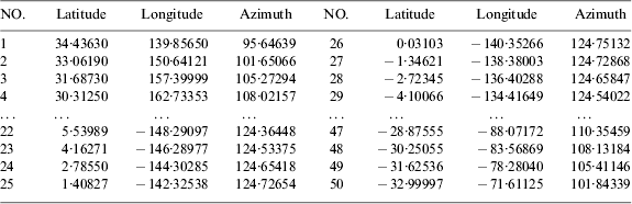
As one can see from Table 3, our method converges very quickly after the first few iterations. The Δλ change of the calculated longitude difference and the given λ ₁₂ also converge very quickly. In the computer program designed by us, the tolerance is set to 10⁻¹⁰ degree, the program designed for geodesic sailing here generates 50 linearly equally spaced points between the two latitudes β ₁ and β ₂, The behaviour of change in longitude decreases as the latitude approaches to the Equator as shown in Table 4.

Table 4.

Waypoints on the geodesic from Yokohama to Valparaiso.