


1. Introduction
Verification of cyber-physical systems (CPS) is challenging as they may deviate from intended behavior due to unexpected environment interference, imprecision of sensors, or simply non-complying implementations. Such deviations may lead to hazardous situations as many CPS, such as unmanned aerial vehicles, may carry out safety critical tasks. For example, the malfunctioning of a drone delivering a package may cause the drone to be out of energy and crash.
It is therefore important to be able to evaluate, at design time, the ability of systems under development to carry out missions as planned despite unexpected events, such as sensor faults or environment perturbations. The system should not deviate from planned behavior, and if a deviation occurs, the system should be able to recover or at least avoid causing harm. For example, if a drone detects that it is too far from a charging station, it should start heading back if necessary. Thus, to carry out missions in unpredictable environments, cyber-physical agents need sufficient sensors to adequately determine their situation and to adapt to unexpected situations.
Given the many different types of faults that may occur, addressing all possible faults by, for example, using better sensors, or with more redundancy, will have great impact on the cost of the system implementation. An alternative approach is to identify at design time faults that the system is unable to deal with. For example, if we can determine that a faulty location sensor can cause the system to be dangerously out of bounds, or fail to meet a critical goal, but a faulty energy sensor does not cause a problem, then more effort can be invested in addressing the faulty location sensor and less effort on addressing energy sensor faults.
Formal methods and tools have been used for verifying the safety (Kamali et al. Reference Kamali, Dennis, McAree, Fisher and Veres2017; Mason et al. Reference Mason, Nigam, Talcott and Brito2017; Mitra Reference Mitra2021; Moradi et al. Reference Moradi, Asadollah, Sedaghatbaf, Causevic, Sirjani and Talcott2020; Sha et al. Reference Sha, Al-Nayeem, Sun, Meseguer and Ölveczky2009) and security (Dantas et al. Reference Dantas, Nigam and Talcott2020) of CPS. While some works investigate the effect of faults (or attacks) on some aspects, such as communication delays, they do not propose systematic means to identify causes for deviations.
The main goal of the work presented in this paper is to enable the use of formal methods for automated design time discovery of unexpected behavior of CPS operating in environments exhibiting faults or other threats, and determining potential causes for this undesired behavior. This allows designs to be adapted to meet many of the challenges before building and testing them. Our work is intended for use during early stages of design and development. During this phase, the mission that the CPS has to perform is specified, e.g., visit some points (Mason et al. Reference Mason, Nigam, Talcott and Brito2017), or be able to autonomously follow vehicles ahead (Dantas et al. Reference Dantas, Nigam and Talcott2020; Moradi et al. Reference Moradi, Asadollah, Sedaghatbaf, Causevic, Sirjani and Talcott2020). Moreover, high level requirements are developed, e.g., the number of CPS agents required, their energy resources, etc. During the specification of these requirements, it is important to understand/discover as well how faults may affect the capacity of CPSes to accomplish their mission. Footnote 1
We build on the soft agents (
 $\textsf{SA}$
) framework (Talcott et al. Reference Talcott, Arbab and Yadav2015), which is a formal framework for specifying and verifying adaptive CPS using the Maude rewriting logic system (Clavel et al. Reference Clavel, Durán, Eker, Lincoln, Martí-Oliet, Meseguer and Talcott2007; Meseguer Reference Meseguer1992). In soft agents, both agent state and the environment are modeled by separate collections of logical assertions called knowledge bases. This supports modeling of both cyber and physical aspects of a system and there interactions. An agents local knowledge base represents its perception of the environment while the environment knowledge base represents ground truth. To specify a CPS model, one needs only specify (i) the logic used by agents to make decisions about actions to perform based on local knowledge and sensing the environment and (ii) the laws determining how the environment is changed by agent actions. The SA framework provides useful data structures and rules for execution to study how system configurations evolve over time.
This paper presents the following contributions:
-
— Formalized Fault Models: We extend
 $\textsf{SA}$
with fault models that may be associated with sensors and actuators. Fault models specify probabilistic distributions on the rate of faults, both erroneous faults, e.g., wrong measurements, and loss faults, e.g., loss of sensors. From the fault specifications, our machinery can execute
$\textsf{SA}$
specifications in which faults may occur.
$\textsf{SA}$
distinguishes the agent’s view of the world specified by its local knowledge base and the (model of) actual world, the environment knowledge base. The effects of fault models in the operational semantics of soft agents specifications lead to mismatches between an agent’s local knowledge base and the environment knowledge base.
-
— Formalized Behavior Requirements as Protocols For the purpose of understanding the impact of faults and other environmental perturbations on the behavior of a CPS, we want a specification that captures both a high level plan and conditions that should hold. Thus, we wanted a language more abstract than rewrite rules, but more operational than temporal logics. We took inspiration from protocols used in regulated collaborative systems (Kanovich et al. Reference Kanovich, Kirigin, Nigam, Scedrov, Talcott and Perovic2017) such as clinical trials. For this purpose, we define a protocol specification language. A protocol specifies which events are expected to happen during a correct execution of a mission; timing constraints to be satisfied by the agents in the form of arithmetic conditions on the time and other parameters of events, e.g., the time between performing action a and action b shall be less than ten time units; constraints on the protocol events; and invariants that shall be preserved, e.g., the energy of a drone shall always be greater or equal to 35 units. The semantics of protocols is given by defining when an execution trace satisfies a protocol. This is done by extracting an event log from an execution trace, i.e., relevant knowledge items accumulated in the execution trace, and checking if the event log satisfies the protocol. The latter problem is solved by mapping it to a satisfaction problem in the language of an SMT-solver.
-
— Cause Diagnosis Workflow: We propose a workflow for determining the cause of failure to satisfy a protocol. Our approach is inspired by recent work on fault ascription based on counterfactual analysis (Gössler and Stefani Reference Gössler and Stefani2016, Reference Gössler and Stefani2020; Laurent et al. Reference Laurent, Yang and Fontana2018). If an execution fails to satisfy a protocol, the associated events determine a set of observable protocol deviations – events that violate protocol constraints or missing events. To check whether a given set of (unexpected) events causes an observed deviation, one asks “if these events had not happened, would the deviation still have occurred?” If not, then indeed the given events can be considered a cause. Otherwise, there must be another set of events to blame. The workflow generates an execution log from a given
$\textsf{SA}$
specification including its fault models, extracts an event log from the execution log, and verifies whether there are deviations using SMT solving to check satisfaction of the protocol. If there are protocol deviations, then we carry out gedanken experiments. Using information about the maximal subprotocol that is satisfied, provided by the SMT solver, and the occurrences of faults identified by execution steps that deviate from the model prediction, we identify a candidate fault. The gedanken experiment re-executes the trace from the point exactly before the candidate fault happened. If the resulting execution satisfies the protocol, then the candidate fault is a cause for the deviation. If not, we proceed by carrying out another gedanken experiment by proposing an earlier fault as candidate.


To the best of our knowledge, the proposed framework is the first executable formal model that uses such protocols to specify desired behavior of CPS and a combination of SMT constraint solving and counterfactual-like reasoning for the diagnosis of deviations. Using the proposed workflow can help design a more robust and efficient system by identifying the faults that are likely to lead to deviations.
This paper starts in Section 2 by giving an overview of the soft agents framework and the running example, called BotTeam, we will be using to illustrate our machinery. After a short introduction to rewriting logic and Maude syntax in Section 3, Section 4 describes more precisely the Soft Agents framework. The main contributions of the paper, listed above, are described in the sections that follow Section 4. Section 5 presents an extension of the soft agents framework with fault models. Section 6 defines the language for specifying protocols and its semantics, while Section 7 defines protocol deviations. Section 8 presents algorithms and a workflow for identifying causes for deviations. Section 9 describes a collection of experiments based on the BotTeam example. Finally, Sections 10 and 11 conclude by discussing related and future work.
2. Soft Agents Overview and Running Example
The soft agents (
 $\textsf{SA}$
) framework provides an architecture and basic functions for defining executable models of
 $\textsf{SA}$
systems. The framework is formalized in the Maude rewriting logic language (Clavel et al. Reference Clavel, Durán, Eker, Lincoln, Martí-Oliet, Meseguer and Talcott2007) and supports exploration of designs (agent strategies) and evaluation in environments with different uncertainties and forms of interference using generic fault models. Key features include
-
— explicit representation of both the cyber (decision making) and physical (using sensors and actuators) aspects of a soft agents CPS,
-
— use of partially ordered knowledge items to represent state, both agent and environment,
-
— soft constraints to support local adaptability by evaluating possible actions in the context of goals, priorities, and local sensor information.
A system configuration consists of one or more agents and one environment object. Each agent has a local knowledge base (KB). This KB can include results of observations (reading sensors), goals, priorities, and information shared by other agents. It is the knowledge an agent uses to make decisions. The environment object also has a KB. This KB is intended to model what holds in the physical world, including agent’s physical state, the surrounding environment (which may include resources, obstacles, etc.), and models for physical actions (including fault models).
Two rewrite rules define the execution/operational semantics of an
 $\textsf{SA}$
system model. The rules depend on interface functions that need to be defined for each model. The doTask rule executes the agent’s decision-making process. The timeStep rule executes actions proposed by the decision processes, carries out information sharing, and advances time. The timeStep rule also has hooks to be used for model specific instrumentation of the execution, for example, recording a log or adding metadata needed to compute properties of interest.
Once model specific interface functions have been defined, the behavior specified by an initial configuration can be explored by using the rewrite command to see one possible execution, using strategy controlled rewriting to explore executions of particular interest, or using search to carry out various forms of reachability analysis.
A consequence of the separation of cyber and physical aspects, the logical model of the physical aspects can be replaced by a simulator, or potentially even by hardware as done in Choi et al. (Reference Choi, McCarthy, Kim and Stehr2013).
2.1 BotTeam example
We will use a simple, yet nontrivial running example, called BotTeam, to illustrate the
 $\textsf{SA}$
machinery throughout the paper. The BotTeam case study was designed to explore simple coordination in the presence of faults. Here we describe the protocol that the agents should follow informally and introduce the model specific components for the BotTeam. Experiments applying fault models and diagnostics will be summarized in Section 9.
The BotTeam consists of two bots with different roles, an initializer, called
 $\textsf{BotI}$
, and a finisher, called
 $\textsf{BotF}$
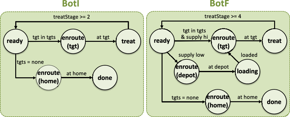
. The high-level specification of the BotTeam case study involving two bots is depicted in Figure 1. Both bots are given a set of locations that requires treatment, e.g., some maintenance work. A treatment consists of a sequence of 4 treatment stages/steps, the first two done by
 $\textsf{BotI}$
, and the last two stages by
 $\textsf{BotF}$
.
The mode automaton for the two bot classes:
 $\textsf{BotI}$
, the initializer, an
 $\textsf{BotF}$
, the finisher. In both cases, the starting state is the
 $\textsf{ready}$
state.

More precisely,
 $\textsf{BotI}$
starts in the
 $\textsf{ready}$
mode. It moves to mode
 $\textsf{enroute(tgt)}$
by selecting one location target,
 $\textsf{tgt}$
, that needs treatment. Once the target location is reached,
 $\textsf{BotI}$
moves to
 $\textsf{treat}$
mode and carries out the first two stages of the treatment. When all target locations are treated,
 $\textsf{BotI}$
enters the mode
 $\textsf{enroute(home)}$
, heads back to the home station, and once reached enters mode
 $\textsf{done}$
.
 $\textsf{BotF}$
follows the same modes of operation as
 $\textsf{BotI}$
. A difference is that
 $\textsf{BotF}$
requires supplies in order to carry out its treatments. Therefore, whenever the supply is low, then
 $\textsf{BotF}$
returns to the depot to re-supply. We also assume, not explicitly shown in the mode automation, that the bots also divert to the charging station whenever their battery level reaches dangerously low level.
Examples of protocol deviations that can be formalized using our machinery include
-
— Wrong Order Treatment Deviation:
$\textsf{BotF}$
carries out a treatment on a target that was not previously treated by
$\textsf{BotI}$
; -
— Delay Between Treatment Deviation:
$\textsf{BotI}$
and
$\textsf{BotF}$
treat a target at times
$t_I$
and
$t_F$
, respectively, such that
$t_F > t_I + \Delta$
, for some
$\Delta > 0$
, i.e.,
$\textsf{BotF}$
treated a target too late. -
— Treatment without Supply Deviation:
$\textsf{BotF}$
attempts a treatment without actually having the necessary supplies. -
— Low Energy Deviation:
$\textsf{BotI}$
or
$\textsf{BotF}$
have energy too low to enable them to return to the charging station to re-charge.


Notice that deviations may involve timing aspects, as in Delay Between Treatment Deviation, or quantitative values, as in Low Energy Deviation and Treatment without Supply Deviation. In the following, we will focus on delay and energy deviations.
To carry out the assigned task of treating target and avoid deviations, the bots make use of their sensors. We assume that each bot has the following sensors: Location Sensor: This sensor reports the location of the bot. Energy Sensor: This sensor reports the current energy level of the bot. Supply Sensor: This sensor reports the current level of supplies available. (This is only used by
 $\textsf{BotF}$
.) Treatment Sensor: This sensor reports whether a target has been treated and up to which stage. Obstacle Sensor: This sensor reports locations of obstacles if any, e.g., a bot at an adjacent/close location. These sensors may be faulty. For example, the location sensor may provide a location reading that does not correspond to the actual location of a bot. This means that the information used by bot to decide how to act may be incorrect, and therefore, the bot does not act as specified by the expected behavior, resulting in a deviation.
3. Rewriting Logic and Maude
The soft-agents framework as well as the detection and diagnosis machinery is specified in Rewriting Logic (Meseguer Reference Meseguer1992, Reference Meseguer2012) and implemented in Maude (Clavel et al. Reference Clavel, Durán, Eker, Lincoln, Martí-Oliet, Meseguer and Talcott2007). We review and illustrate Rewriting Logic and Maude next.
Rewriting logic is a logical formalism that is based on two simple ideas: (i) states of a system are represented as elements of an algebraic data type, specified in an equational theory and (ii) the behavior of a system is specified by local transitions between states described by rewrite rules. An equational theory specifies data types by declaring constants and constructor operations that build complex structured data from simpler parts. Mathematical structures such as sets and maps can be represented directly by declaring, using axioms that the constructors are associative and commutative, and naming the identity element. Functions on the specified data types are defined by equations that allow the result of applying the function to be computed. A term is a variable, a constant, or the application of a constructor or function symbol to a list of terms.
A rewrite rule has the form
 $t \Rightarrow t'~\mathit{if}~c$
, where t and t’ are terms possibly containing variables and c is a condition (a Boolean term). For a system in state s, such a rule is enabled if t can be matched to a part of s by supplying the right values for the variables (using a matching substitution), and if the condition c holds when supplied with those values. In this case, the rule can be applied by replacing the part of s matching t by t’ using the matching values for the place holders in t’. The process of application of rewrite rules generates computations (and traces).
Maude is both a language and tool based on rewriting logic (Clavel et al. Reference Clavel, Durán, Eker, Lincoln, Martí-Oliet, Meseguer and Talcott2007; Maude-Team 2021). Maude provides a high-performance rewriting engine featuring matching modulo associativity, commutativity, identity axioms, and search and model-checking capabilities. Thus, given a specification S of a concurrent system, a user can execute S, using one of Maude’s built-in rewriting strategies, to find one possible behavior; use search to see if a state meeting a given condition can be reached; or model-check S to see if a temporal property is satisfied, and if not to see a counter-example computation. Maude also supports reflection with a simple representation of modules and their components, and access to key functions of the core Maude system that allow the user to specify execution and search strategies and module transformation.
We introduce the syntax of Maude with a simple example with a bot moving on a grid. First, we define the sorts as follows:
sorts Bot Bot? .
subsort Bot < Bot? .
In particular, the first line specifies two sorts Bot and Bot? and the second line specifies that Bot is a subsort of Bot?. Footnote 2
We use operators to populate these sorts as follows:
op noB : -> Bot? [ctor] .
ops B0 B1 : -> Bot [ctor] .
where noB denotes the absence of a Bot, while B0 and B1 are two bot names.
Similarly, we can define square(s) (of the grid) as follows:
sorts Square Squares .
subsort Square < Squares .
op sq : Nat Nat Bot? -> Square [ctor] .
op none : -> Squares [ctor] .
op __ : Squares Squares -> Squares [ctor comm assoc id: none] .
Notice the keywords comm, assoc and id:. They denote that an operator is commutative and associative, with identity none. Thus Squares is a multiset of elements of sort Square.
Footnote 3
Based on these sorts and operators, we can define a scenario with one bot on a
 $3 \times 3$
grid as follows:
op scenario : -> Squares .
eq scenario =
    sq(0,0,B0) sq(0,1,noB) sq(0,2,noB)
    sq(1,0,noB) sq(1,1,noB) sq(1,2,noB)
    sq(2,0,noB) sq(2,1,noB) sq(2,2,noB) .
where scenario denotes that bot B0 is at position (0,0) and the remaining locations are empty.
So far, we have used an equational theory to define the datatypes used by rewrite rules. The following is an example of a conditional rewrite rule:
crl[mv]:
  sq(i0,j0,b:Bot) sq(i1,j1,noB) => sq(i0,j0,noB) sq(i1,j1,b:Bot)
if ((i1 == s i0) or (i0 == s i1) or
        (j1 == s j0) or (j0 == s j1) ) .
This rule specifies that a bot at any position (i0,j0) can move to upward, downward, to the left or right, as long at it it remains on the board. This is specified by the conditions of the rule where s is the successor function.
With the specification above, we can use Maude’s search engine to check for reachability properties. For example, the following command
search [1] scenario =>+ sqs:Squares sq(2,2,B0) .
checks whether the bot B0 can reach the position (2,2). Maude reports a solution where position (0,0) is now empty (noB) and B0 is indeed at position (2,2).
For more details on Maude and Rewriting Logic, we refer the interested reader to Clavel et al. (Reference Clavel, Durán, Eker, Lincoln, Martí-Oliet, Meseguer and Talcott2007).
4. Soft Agents Framework
We will use the BotTeam scenario to illustrate key elements of the soft agents formalization in Maude. The basic soft agents framework is described in more detail in Talcott et al. (Reference Talcott, Nigam, Arbab and Kappe2016) and the technical report accompanying the code (Kim et al. Reference Kim, Mason and Talcott2019).
4.1 Basic sorts and functions
Soft agents uses the following basic sorts:
Id is the sort of identifiers, used to identify agents, and other objects. Each model is responsible for defining its own Id constructors. The BotTeam Id constructors are b(i:Nat) (bots), st(i:Nat) (stations), dp(i:Nat) (depots), and ob(i:Nat) (obstacles). A constant eI of sort Id is declared to name the unique environment object in a system configuration.
Time is the sort used to represent time. The soft agents framework provides a variety of time modules to choose from, including discrete (natural numbers) or dense (rationals or reals) time representations. In the current soft agents framework instances, we use discrete time represented using the sort Nat of natural numbers.
The sort Loc is an interface sort at the framework level. There is a constant noLoc indicating an unknown location. In the Bot example, locations are points on a two-dimensional grid using the following sorts and constructors:
sort Pt2 . subsort Pt2 < Loc . op pt : Nat Nat -> Pt2 [ctor] .
For example, pt(2,1) specifies the location (2,1) on a two-dimensional grid.
Class is the sort of object classes.
A KB (sort KB) is a set of knowledge items (sort KItem). There are two (sub)sorts of knowledge items, persistent (sort PKItem), and transient (sort TKItem). Transient knowledge items are time stamped information items of the form info:Info @ t:Time where terms info:Info are expected to have parameters that change over time. Persistent knowledge items model properties that do not vary over time and thus are not time stamped. There is a distinguished knowledge item clock(t:Time) that represents the current time. For example, clock(10) represents that 10 time units have passed since the starting time 0. There are two additional built in knowledge item terms. class(id:Id,cl:Class) says that the class of the entity (agent or other object) with identifier id:Id is cl:Class. It has sort PKItem as the class is not expected to change. For example, class(b(0),BotI) says that the entity with identifier b(0) is an initializer bot, BotI. The term atloc(id:Id,l:Loc) @ t:Time denotes that the entity with identifier id:Id is at location l:Loc at time t:Time. It has sort TKItem since in the case of a mobile entity l:Loc changes as the agent moves.
The local knowledge base (lkb) of a particular agent and the environment knowledge base (ekb) are of the sort KB. The former specifies the agent’s view of the world, obtained from its possibly faulty sensors, while the latter is the actual specification of the world.
We classify as background knowledge the items in a knowledge base that specify the general conditions of the scenario. Typically, the background knowledge contains data that does not change, e.g., the types of agents, the locations of stations.
Example 4.1. The following local knowledge base of the initializer, lkbI, specifies that its Id is b(0), it is at location (0,1); the station st(0) is at the location (3,2); its energy is 100 units; it is in mode
 $\textsf{ready}$
.
lkbI = clock(0) class(b(0),BotI) class(st(0),Station) (atloc(b(0),pt(0,1)) @ 0)
  (atloc(st(0),pt(3,2)) @ 0)(mode(b(0),ready) @ 0) (energy(b(0), 100) @ 0)
  (ereserve(b(0),35) @ 0) home(b(0),pt(0,1)) (targets(pt(4, 0) ; pt(5, 4)) @ 0)
   (fence (b(0),pt(0,0),pt(6,5)) @ 0)
The KItem (mode(b(0),ready) @ 0) specifies that the bot is ready for carrying out the tasks assigned, namely, visit the points in (targets(pt(4, 0) ; pt(5, 4)) @ 0). The background knowledge of b(0) is
class(st(0),Station) (atloc(st(0),pt(3,2)) @ 0)class(b(0),BotI)
home(b(0),pt(0,1)) (fence (b(0),pt(0,0),pt(6,5)) @ 0) (ereserve(b(0),35) @ 0)
The KItem (ereserve(b(0),35) @ 0) is a parameter used by the soft constraint solving mechanism to cause a Bot to pass by the charging station before its energy level gets too low. It is part of the scenario specification rather than representing state that evolves over time, and thus background knowledge. The (targets(pt(4,0) ; pt(5,4)) @ 0) KItem is the list of locations to be visited. When a target is selected it is removed from the list and made the current target. When there are no more targets and the current target has been treated, the Bot goes home using the home(b(0),pt(0,1)) KItem to remember where that is.
Elements of the sort Sensor name sensors available to an agent. The Bot sensors described in Section 2 are associated to the constants locS, energyS, obstacleS, and treatS, respectively. The finisher Bot also has a supply-level sensor with associated constant supplyS.
The sort Task represents tasks to be carried out by agents. Task events are executed by the doTask rule. In our case studies, only one task is used, namely tick. It is used to schedule the next time the agent reads its sensors and proposes actions.
Events are used to determine what happens during rule application. The sort Event has two subsorts: DEvents that are actions (sort Action) or tasks (sort Task) with delays, and IEvents that are events to be processed immediately (implicit delay of 0).
The sort Action is used to describe actions proposed by agents. Each action has an identifier parameter that identifies the agent carrying out the action and possibly other parameters. Each action consumes resources, such as energy, which are specified by the operational semantics of the scenario described in Section 4.2.
Example 4.2. The actions available to BotTeam agents are
-
— charge(id:Id) increases energy level provided the bot is at the supply depot.
-
— mv(id:Id,dir:Pt2) moves one unit in the direction specified by the vector dir:Pt2.
-
— treat(id:Id) increments treatment stage by 1. For BotF, the execution of this action uses some of the supply.
-
— load(id:Id) available to BotF at the supply depot to replenish its supply.
To decide its next action, an agent ranks each applicable action in its current local knowledge base according to the agent’s preference specified using soft constraints (Bistarelli et al. Reference Bistarelli, Montanari and Rossi1997). The result is a set of ranked actions, ract, which are pairs of the form {rval,act}, where act is the action and rval is the action’s valuation, typically a value in the interval [0,1], where 1 is more preferred.
4.2 Soft agents semantics: Configuration and rules
A soft agents configuration (sort Conf) is a multiset of configuration elements (sort ConfElt). Agent objects (sort Agent) and environment objects (sort Env) are configuration elements. Formally Agent and Env are subsorts of ConfElt. A well-formed configuration needs a unique environment object and at least one agent object. Other configuration elements can be defined to control execution and to track properties of interest. Logs and bounds on the time or number of applications of selected rewrite rules are examples of other configuration elements as we will see later. Configurations are open ended as you can add or remove an element and still have a configuration. A soft agents system conf:Conf (sort ASystem) specifies exactly which configuration elements are present by enclosing them in s. The use of ASystem is required when a rewrite rule needs to know it has all elements of a configuration under consideration, in contrast to rules that operate on one or a pair of configuration elements.
An agent object has the form [id:Id : cl:Class | attrs:AttributeSet] where an attribute is a key-value pair. Agent objects must have at least the following attributes: lkb : localkb:KB, the agent’s local KB; sensors : ss:SensorSet, the agent’s sensors evs : events:Events, events awaiting processing ckb : cachedkb:KB, cached knowledge to be shared.
Example 4.3. The following is an example of an Agent Object for the BotI class where lkbI is taken from Example 4.1 and the sensors are as described in Section 4.1
[b(0) : BotI | lkb : lkbI, ckb : none,
              sensors : (locS obstacleS energyS treatS), evs : (tick @ 0)]
An environment object has the form [eid:Id | ekb:KB] The environment KB (ekb:KB) contains information about the physical state of each agent such as location and energy, information about resources such as location of charging stations, information about obstacles, global parameters such as communication range, and fault models. The environment KB and each agent local KB contain a clock knowledge item.
The semantics of an soft agents configuration is defined by two rewrite rules: doTask and timestep described in the following.
4.2.1 Rule doTask
The doTask rule applies to subconfigurations involving a single agent object as it has no need to know all the configuration elements of a system. Formally, this rule applies to any agent with a task that has 0 delay ((task @ 0)) as specified below:
Footnote 4
crl[doTask]:
  [id : cl | lkb : lkb, evs : ((task @ 0) evs), ckb : ckb, sensors : sset, ats]
  [eid | ekb]
=> [id : cl | lkb : lkb', evs : evs', ckb : ckb', sensors : sset, ats][eid | ekb']
  if t := getTime(lkb)
  /\ {ievs,devs} := splitEvents(evs,none)
  /\ {skb,ekb'} := readSensors(id,sset,ekb)
  /\ kekset := doTask(cl,id,task,ievs,devs,skb,lkb)
  /\ {lkb', evs', kb} kekset0 := selectKeK(lkb,kekset)
 /\ ckb' := addK(ckb,kb) .
The doTask rule uses the following functions:
splitEvents splits its first argument into two sets, the immediate events ievs and the events with delays devs. The agent processes ievs. It may modify devs, but usually just adds new tasks and/or actions.
readSensors returns the union skb of the result of reading each sensor in sset independently, together with an updated environment. To read a single sensor, the sensor knowledge is retrieved from the environment KB along with a fault model for that sensor, if any. If there is no fault model, the sensor knowledge is returned. If there is a fault model, it is applied using applySensorF(id,s:Sensor,skb0,fkb,ekb) where skb0 is the sensor knowledge and fkb is the fault model. The environment update is an artifact of how fault models are applied using Maude’s random number generator. Fault models and their application are discussed in Section 5. As an example the knowledge associated to the location sensor locS of a Bot with identifier b(0) has the form atloc(b(0),loc:Loc) @ t:Time.
The doTask function specifies the possible actions that the agent is willing to do, given its current set of tasks, events (immediate and delayed), sensed information, and local knowledge base. It returns a set of triples of the form lkb’,evs’,kb where lkb’ is the agent’s new local KB, evs’ updates the pending events, and KB is new information to share. The set arises because there maybe more than one choice of action that the soft constraint solver views as acceptable.
Example 4.4. For example, the doTask rule applied to the agent object described in Example 4.3 (and the corresponding environment object) results in the Bot b(0) updating its evs to (tick @ 1) (cv(100),u(1),mv(b(0), pt(1, 0)) @ 0) specifying that the bot decided to move north with the highest preference cv(100),u(1). This is achieved by first determining using splitEvents the immediate events and the delayed events. In this example, there is only the immediate event tick @ 0 and no delayed event. Then the function readSensors probes the environment knowledge base using the sensors (locS obstacleS energyS treatS). This means that the variable skb in the doTask rule contains the new location, obstacles, energy, and treated knowledge (with errors introduced by fault models). The the function doTask evaluates which action to take, which in this case is to move north. Footnote 5
4.2.2 Rule timeStep
Intuitively, the timeStep rule advances time carrying out the actions that have been decided by each agent as specified by the doTask rule. So it is only applicable when doTask is no longer applicable. Since the rule needs to know all configuration elements it applies to systems, aconf as specified below:
crl[timeStep]: { aconf } => { aconf2 }
  if nzt := mte(aconf)
  /\ t := getTime(envKB(aconf))
  /\ evs := effActs(aconf)
  /\ ekb0 := doEnvAct(t,nzt,envKB(aconf),evs)
  /\ ekb' := resolveKB(getEnvId(aconf),ekb0,envKB(aconf))
  /\ aconf0 := updateEnv(ekb',timeEffect(aconf,nzt))
  /\ aconf1 := shareKnowledge(aconf0)
  /\ aconf3 := updateLog(aconf1,t,nzt,evs)
  /\ aconf2 := updateConf(aconf3) .
where mte computes the time of the next scheduled task. So when it returns a nonzero time, it means that doTask is not applicable.
effActs(aconf) computes the set of action events in each agents evs attribute.
Actions in evs are carried out concurrently by doEnvAct(t,nzt,envKB(aconf),evs), producing updates for the environment KB. This function also implements action faults discussed in Section 5.
Example 4.5. When doEnvAct is applied to the events shown in Example 4.4 it returns an ekb’ where the position of the b(0) is (atloc(b(0),pt(1,1)) @ 1), instead of the position (atloc(b(0),pt(0,1)) @ 0). That is the agent moves north.
resolveKB(getEnvId(aconf),ekb0,envKB(aconf)) produces a consistent global update. In the current models, the only conflicts are when two or more agents want to move to the same position. This is resolved by choosing one of the agents to succeed, the others must stay where they started. Footnote 6
timeEffect(aconf,nzt) advances time in the configuration aconf by nzt, and the environment KB in the resulting configuration is updated using the function updateEnv and ekb’.
shareKnowledge is used to enable the communication between agents. It considers the ckb attributes for each pair of agents that are within the model’s communication distance, computes what is new from each agent’s perspective, updates the caches, and adds rcv(newkb) to the agent’s evs attribute.
updateLog and updateConf are hooks to allow for instrumenting configurations. Execution logs are a common form of instrumenting executions. The soft agents framework provides a data structure and parametric procedure to collect log information. A log (sort Log) is a sequence of log items with elements of the sequence separated by ;. In our case studies where the time to pass (nzt) is 1, updateLog(aconf1,t,1,evs) returns aconf1 if aconf1 has no log element. Otherwise it adds to the log a logitem t:Time,acts,lconf:Conf where acts is the actions with delay 0 in evs and lconf is computed by the interface function kblog(aconf1,none) (the none is the initial value of the configuration element accumulator).
The default for updateConf is to return its argument unchanged. The soft agents framework provides a configuration element bound(n:Nat) to limit the number of timeStep rule applications.
4.3 Executions
Using the two rewrite rules, doTask and timeStep, executions of a soft agents system alternate steps where agents observe (read their sensors) and decide on actions, and steps where the actions are realized by the environment. Assuming a set of agents,
 $a_1, \ldots, a_n$
, an execution step is a sequence of transition segments of the form
 \begin{equation*} \mathcal{C}_0 \longrightarrow[\texttt{doTask}(a_1)]~ \mathcal{C}_1 \longrightarrow[\texttt{doTask}(a_2)]~ \cdots \longrightarrow[\texttt{doTask}(a_n)]~ \mathcal{C}_n \longrightarrow[\texttt{timestep}]~\mathcal{C}'\end{equation*}
with a sequence of applications of doTask
 $(a_i)$
applied to an agent
 $a_i \in \{a_1,\ldots,a_n\}$
followed by an instance of the timestep rule. We will abbreviate any such sequence as
 \begin{equation*} \mathcal{C}_0 \longrightarrow[\texttt{doTask}]~ \mathcal{C}_n \longrightarrow[\texttt{timestep}]~\mathcal{C}'.\end{equation*}
An execution trace is a sequence of execution steps.
The Maude implementation of the soft agents framework, case studies, sample output of executions and searches, and documentation is available at
github.com/SRI-CSL/SoftAgentsDiagnosis.git.
It is possible to use Maude rewriting and search machinery to carry out experiments and analysis.
Example 4.6. (Using search to check energy-level compliance) We illustrate using the search capability to look for situations in which the BotTeam fails to meet the energy caution invariant: a bots energy should not go below 35%. In the case of two targets to maintain and no faults the initial state is described by the term mkInitS(pt(4, 0) ; pt(5, 4), true).
The command to search for one example of non compliance by the finisher bot b(1) is
search [1] mkInitS(pt(4, 0) ; pt(5, 4), true) =>+
   {aconf:Conf [eI | ekb:KB ]} such that getEnergy(b(1),ekb:KB) < 35 .
and the result is No solution. This means that in the absence of faults, the energy of b(1) is not lower than 35.
5. Fault Models
This section introduces a general mechanism, called fault models, for adding faults to a soft agents system model. The fault models serve two purposes. One purpose is to provide a setting for developing detection and diagnosis methods. Another purpose is to support exploring the design space for soft agents behavior in terms of resilience and adaptability in the presence of imperfect sensors and actuators and unpredictable environment perturbations. There are two kinds of fault, sensor faults and action faults, which we describe in the following. Environment perturbations such as obstacles are modeled as knowledge items in the environment KB. Suitable sensors are needed to detect these perturbations, which can be faulty.
There are three sorts used to parameterize fault models: FType, FVal, and FPars.
FType is the sort of fault types. The soft agents framework currently provides two sensor fault types: a boolean fault type, boolFT, a fault that is either present or not; and a simple fault type, simpleFT, with fault effect parameterized by elements of sort FPars. FVal provides a super sort for collecting parameters with different structures.
The parameters for a fault of type boolFT are terms of sort FPars of the form bFP(bp:Rat) where bp:Rat specifies the probability of a fault. The parameters for a fault of type simpleFT are terms of sort FPars of the form sFP(fp0:Rat,fp1:Rat,fv:FVal). The two rational arguments, fp0:Rat,fp1:Rat, are typically used as probability thresholds, such as, determining if a sensor is broken (no reading) or not, and if not broken whether there is a reading error. The FVal argument is an interface sort. Each soft agents model and sensor will have its own subsorts.
Sensor faults can model imprecision of sensors, broken sensors, environmental interference such as mud on a camera or interference with a GPS signal. A sensor fault is specified by a term of sort Info of the form sF(id:Id,s:Sensor,ft:FType,fp:FPars) where id:Id is the identifier of the agent whose sensor s:Sensor is faulty.
Example 5.1. The term sF(b(0),locS,simpleFT,sFP(1/10,1/5,ptV(pt(0,1)))) specifies a simple location sensor fault for Bot b(0). With probability
 $1/10$
the sensor gives no reading (noLoc) and if it gives a reading, the reading is off by 1 unit north with probability
 $1/5$
. The meaning of the fault term is given by the readSensors function.
The interpretation of a sensor fault model is defined by the function
applySensorF(id:Id,s:Sensor,skb:KB,fm:KB,ekb:KB)
which is invoked by the readSensor function as described in Section 4.2.1. id:Id is the identifier of the agent reading its sensors, s:Sensor is the sensor being read, skb:KB is the sensor information in the absence of faults fm:KB is the fault model to apply, and ekb:KB is the environment KB where the sensor is being read. The result is a pair of KBs, the faulty sensor knowledge and the updated environment KB. applySensorF uses Maude’s builtin randon number sequence generator to sample the various fault probablility distributions. Each agents is allocated a subsequence and the environment KB records the agent’s position in its subsequence. The updated environment KB records the new random sequence positions for each agent.
Action faults can be used to model action imprecision or failure, environmental interference such as wind blowing a drone or a steep hill reducing the effectiveness of a move action. Similar to sensors, we need names for action types. The sort Act is the sort of action (type) names. In the BotTeam example the names are mvA (move action), chargeA (charge action), treatA (treat action), and loadA (load action, for the finisher bot). Similar to sensor faults, an action fault is specified by terms aF(id:Id,a:Act,ft:FType,fp:FPars) of sort Info.
Example 5.2.
aF(b(0),mvA,simpleFT,sFP(1/10,1/10,ptV(pt(-1,0)))) specifies a move action fault for Bot b(0) with probability
 $1/10$
of a broken actuator (no move), probability
 $1/10$
of a faulty move, if the actuator is not broken, with error given by the vector pt(-1,0).
As discussed in Section 4.2.2, the interpretation of an action fault model is defined by the doEAct function. It returns an update to the environment KB that may include execution deviations. The occurrence of such deviation depends on the probability distributions specified by the given fault-models.
6. Protocols: Formal Behavior Requirements
In order to detect when something goes wrong in an SA system, one needs to know what is right. Furthermore, to find the cause when a goal is not achieved or a requirement/invariant is not satisfied it helps to have some idea of the steps expected to lead to success, for example, a mission plan. To identify where in the mission plan things went wrong, it is important to have a formal representation of the plan and its constraints. Correct execution of a mission plan may achieve higher level goals, but that is not the issue being addressed here. It might be possible to encode relevant features of a mission plan in a temporal logic. We felt that a direct formalization would be simpler and easier to understand and validate.
Inspired by rules for carrying out scientific experiments and clinical trials (Kanovich et al. Reference Kanovich, Kirigin, Nigam, Scedrov, Talcott and Perovic2017), we propose the notion of soft agents protocol to specify desired/required behavior of a soft agents system. Intuitively, a protocol specifies a finite mission as in the BotTeam example described in Section 2. In particular, a protocol specifies observable events that should take place (stages or steps making progress) along with any ordering or timing conditions and possibly other conditions. To allow for flexibility and avoid specifying values, such as exact times, a protocol consists of a set of observable event patterns and constraints expressed in terms of pattern variables, together with invariant constraints (defining what is called adverse events in clinical trials).
Given a protocol, we associate notion of compliance or satisfaction – when does an execution of a soft agents system meet the requirements specified by that protocol. Using the intuition above, the idea is to match protocol event patterns to observable events of the execution and then check that the instantiated constraints hold.
Intuitively, protocol specifications are artifacts produced between system specification, e.g., expressed as Linear Temporal Logic (Pnueli Reference Pnueli1977) formulas, and the development of executable models, such as those using SA framework. The purpose of protocols is to enable analysis of how things may go wrong based on fault models and the executable models as we detail in Section 7.
6.1 SA protocols
A soft agents protocol is a finite partial order of observable event patterns together with constraints on the pattern variables and possibly additional invariant constraints independent of the event pattern variables. Using event patterns rather than concrete events allows for compact specification and also for specifications that can be met under many conditions. For example, there is no need to specify concrete times for events, when relative times and time intervals are what is important; one may not want to specify precise locations, but only neighborhoods; and in some cases, the order between a pair of events may not matter as long as both happen.oft agents event patterns are represented by symbolic knowledge items, i.e., time stamped information items where the time stamps are variables, and the parameters of the information part may be variables. The partial order is specified by ordering relations on the time stamp variables. We require that each event has a unique symbolic time stamp. Thus, a symbolic event can be identified by its time stamp and so multiple occurrences of the same information template can be distinguished. Invariants are typically used to represent safety envelopes, such as maintaining energy above a given minimum level or ensuring that the distance between pairs of agents is greater than a given minimum.
Definition 6.1.
(SA Protocol) For a system with agents whose identifiers are the elements of AgentIds, a (soft agent) protocol
 $\mathcal{P}$
is a tuple
 $(\mathit{TL}, \mathit{Eps}, \mathit{LO}, \mathit{GO}, \mathit{CS},\mathit{Inv})$
where
-
—
$\mathit{TL}$
is a list of timelines, where the timeline for an agent is the list of time stamp variables for events under control of that agent. -
—
$\mathit{Eps}$
is the set of protocol event patterns. -
—
$\mathit{LO}$
is the set of local order constraints for each agent. A local order constraint for an agent has the form s0:Time < s1:Time where s0:Time, s1:Time are time stamp variables in the timeline for that agent. -
—
$\mathit{GO}$
is the set of global order constraints, s0:Time < s1:Time where s0:Time, s1:Time belong to the timelines of different agents. -
—
$\mathit{CS}$
consists of additional constraints on protocol event pattern variables. -
—
$\mathit{Inv}$
is the set of invariant constraints. These are implications epats => c where epats is a list of event pattern viewed as a conjunction, c is a constraint on the variables of the event patterns in epats.


Example 6.2. (BotTeam Protocol) We describe protocol elements for bot b(0) (Initiator) as introduced in Section 2. Its timeline is
timeline(b(0),s00:Time,s01:Time,s02:Time,s03:Time,s04:Time,s05:Time)
The time stamp variables are used in the event pattern:
atloc(b(0),pt(4, 0)) @ s00:Time treatStage(pt(4, 0),2) @ s01:Time
atloc(b(0),l0:Pt2) @ s02:Time atloc(b(0),pt(5, 4)) @ s03:Time
treatStage(pt(5, 4),2) @ s04:Time atloc(b(0),l1:Pt2) @ s05:Time
This pattern specifies the events to be carried out by the bot, namely, the locations b(0) to be visited and the treatments to be applied.
Local order constraints specify temporal conditions for the protocol. The following local ordering constraint specifies that the timestamps of the events in the pattern above shall form a total order, i.e., one event is followed by the next one.
s00:Time < s01:Time s01:Time < s02:Time s02:Time < s03:Time
s03:Time < s04:Time s04:Time < s05:Time
The local ordering s03:Time - s01:Time < 15 specifies that the bot shall not take too long to reach the second location once the second treatment of the first location is completed.
Global order constraints can specify timing conditions involving multiple agents. For example, treatStage(pt(4, 0),4) @ s11:Time is in the event patterns of bot b(1), and the global order constraint s11:Time - s01:Time < 10 specifies that the time between treatments shall not exceed 10 time units.
The following invariant specifies that the energy levels of the bot shall always be greater than 35 time units: energy(id:Id,e:Nat) @ s:Time => e > = 35
The design of the protocol language has been carefully crafted to enable the development of automated workflows using SMT-solvers and Maude. While we believe that it is possible to extend the language with other constructs such as finite branching and finite unfolding, unbounded recursion will likely lead to undecidability of the diagnosis problem, or to problems that current SMT implementations cannot check satisfiability.
Typically in an execution of the protocol the local order for an agent is a total order. The order need not be totally specified, meaning that multiple orders are acceptable. Some actions may cause change in more than one observable and hence the corresponding events will appear simultaneously.
6.2 Protocol satisfaction by event logs
Not all knowledge items make sense as events. The realization of a protocol event is the result of an agent action, that is it is among the knowledge items returned by doAct or envAct. In particular, for the agents to execute the protocol these events should be under the control of the agents, not environment actions. In the case of the BotTeam protocol events are location, treatment stage, and energy knowledge items. If the bots had cameras, knowledge items relevant to taking pictures could be protocol events.
We define the event language,
 $\mathit{EL}$
, of a protocol to be the knowledge items generated by the information constructors used in the event patterns appearing in the protocol (both the partial order and the invariants). This language is specified by a sub-signature of the Maude KB signature. For example, the event language of the BotTeam above is given by the constructors
atloc : Id Loc -> Info treatStage : Loc Nat -> Info energy : Id Nat -> Info
Definition 6.3
(Event Log) An event log,
 $\mathit{EvL}$
, over a given event language and AgentIds is a concrete set of events, i.e., ground knowledge terms whose information component is in the given language and whose agent identifiers are in AgentIds.
Definition 6.4
(Satisfaction by Event Log) Let
 $\mathcal{P} = (\mathit{TL}, \mathit{Eps}, \mathit{LO}, \mathit{GO}, \mathit{CS}, \mathit{Inv})$
be a protocol for AgentIds with event language,
 $\mathit{EL}$
. Let
 $\mathit{EvL}$
be an event log over AgentIds and
 $\mathit{EL}$
.
 $\mathit{EvL}$
satisfies
 $\mathcal{P}$
(
 $\mathit{EvL} \models \mathcal{P}$
) is defined as follows:
-
—
$\mathit{EvL} \models \mathcal{P}$
if and only if
$\mathit{EvL} \models (\mathit{Eps}, \mathit{LO}, \mathit{GO}, \mathit{CS})$
and
$\mathit{EvL} \models \mathit{Inv}$
. -
—
$\mathit{EvL} \models (\mathit{Eps}, \mathit{LO}, \mathit{GO}, \mathit{CS})$
if and only if there is a substitution,
$\sigma$
, embedding
$\mathit{Eps}$
in
$\mathit{EvL}$
(
$\sigma(\mathit{Eps}) \subseteq \mathit{EvL}$
) such that
$\sigma(\mathit{LO})$
,
$\sigma(\mathit{GO})$
,
$\sigma(\mathit{CS})$
are all true. -
—
$\mathit{EvL} \models \mathit{Inv}$
if and only if
$\mathit{EvL} \models \mathtt{ep => c}$
for each invariant expression ep => c in
$\mathit{Inv}$
. -
—
$\mathit{EvL} \models \mathtt{ep => c}$
if and only if for each instance
$\sigma_0(\mathtt{ep})$
in
$\mathit{EvL}$
,
$\sigma_0(\mathtt{c})$
is true.


Example 6.5. For example, running the BotTeam example in Maude, we obtain an event log of the following form:
(atloc(b(0), pt(0,0)) @ 1) ... atloc(b(0), pt(5,4)) @ 20)
(treatStage(pt(4,0), 2) @ 9) ... (treatStage(pt(4,0), 4) @ 15)
(treatStage(pt(5,4), 2) @ 28) ... (treatStage(pt(5,4), 4) @ 34)
((energy(b(0), 100) @ 1)) ... (energy(b(0), 60) @ 34)
The first line contains the events with positions of b(0) during the execution, while the following two lines contains the treatment events for the two treatment points. The last line contains the bot’s energy levels. This event log satisfies the local constraint s03:Time - s01:Time < 15 described in Example 6.2. Indeed, the time of completion of the second treatment of the location pt(4,0) is nine, i.e., the value s01:Time is nine. Moreover, the time b(0) reached and the second point was 20, i.e., the value of s03:Time is 20. Thus, the constraint s03:Time - s01:Time < 15 is true as
 $20 - 9 = 11 < 15$
.
6.3 Protocol satisfaction by execution traces
In Section 4.2.2, a generic mechanism for collecting execution logs was described. Here we consider logs appropriate for checking satisfaction and detecting deviations from a protocol and derive event logs from these execution logs.ecall that a log item has the form t, acts,lconf where t is a time stamp, acts an action set, and lconf a set of configuration elements. t is the time just before the actions are carried out. A log
 $\mathit{Lg}$
is a sequence of log items with time increasing. We write
 $len(\mathit{Lg})$
for the length of the sequence. Define
 $\mathit{Lg}[t]$
to be the (unique) log item of
 $\mathit{Lg}$
with time stamp t, i.e., the log item of the form t, acts, lconf.
 $\mathit{Lg}[t]$
is nil if there is no such log item. Note that the logs generated by updateLog have a log item for each time from 0 up to (not including) the length of the log.
Here we restrict our attention to logged configurations lconf that have the form [eid | ekbl] … [id : Cl | lkb : lkbl] … In particular, only the lkb attribute of agents is kept. How much of the execution configuration KBs to keep in the log depends on the intended use. If one is only checking protocol satisfaction, then only the knowledge items in the protocol event language are needed. For detecting deviations or diagnosis more information is usually needed. For checking properties other than protocol satisfaction, log items might collect metadata rather than environment and agent knowledge.
We introduce some auxiliary notation used to define the notion of “log for a trace” and satisfaction relations between protocols and traces or logs. In the following,
 $\mathit{Tr}$
is an execution trace as defined in Section 4.3 and
 $\mathit{Lg}$
is a log. For j from 0 up to (not including)
 $len(\mathit{Tr})$
,
 $\mathit{Tr}[j]$
is the
 $j^{th}$
execution step of
 $\mathit{Tr}$
:
 $\mathcal{C}_j \longrightarrow[\mathtt{doTask}]~\mathcal{C}_{j}' \longrightarrow[\mathtt{timestep}]~\mathcal{C}_{j+1}.$
Moreover, let acts.j be the actions carried out in the above timestep rule. Notice that j is the time t in
 $\mathcal{C}_j$
, and
 $j + 1$
is the time in
 $\mathcal{C}_{j+1}$
and we also write
 $\mathit{Tr}[t]$
for this trace element. For t a timestamp of
 $\mathit{Lg}$
,
 $\mathit{Lg}[t]$
is t,acts,lconf where lconf has the form
[eid | ekbl] ... [id : Cl | lkb : lkbl.id] ...
We define the following notation:
 $\mathit{Lg}[t][eid] = \mathtt{ekbl}$
,
 $\mathit{Lg}[t][id] = \mathtt{lkbl.id}$
,
 $\mathit{Lg}[t][a] = \mathtt{acts}$
and letting [eid | ekb] … [id : cl | lkb: lkb.id …] … be the final configuration C.j+1 of
 $\mathit{Tr}[j]$
where
 $j = t$
above, then
 $\mathit{Tr}[t][eid] = \mathtt{ekb}$
,
 $\mathit{Tr}[t][id] = \mathtt{lkb.id}$
,
 $\mathit{Tr}[t][a] = \mathtt{acts.j}$
.
Definition 6.6
(Trace and Logs). Let AgentIds be the identifiers of agents in the initial configuration of
 $\mathit{Tr}$
(and hence of each configuration of
 $\mathit{Tr}$
).
-
A log
$\mathit{Lg}$
is a log for
$\mathit{Tr}$
if
$\mathit{Lg}[j]$
is a log item for
$\mathit{Tr}[j]$
for j a time stamp of
$\mathit{Lg}$
. -
$\mathit{Lg}[t]$
is a log item for
$\mathit{Tr}[t]$
if and only if the following conditions are satisfied
-
—
$\mathit{Lg}[t][eid]$
is a subset of
$\mathit{Tr}[t][eid]$
-
—
$\mathit{Lg}[t][id]$
is a subset of
$\mathit{Tr}[t][id]$
for id in AgentIds
-
—
$\mathit{Lg}[t][a] = Tr[t][a]$
-


Satisfaction of a protocol from the environment and agent perspective for traces and logs is defined by reducing it to associated event logs.
Definition 6.7
(Trace and Log Satisfaction). For a trace
 $\mathit{Tr}$
and a log
 $\mathit{Lg}$
as above
-
—
$\mathit{Tr} \models_E \mathcal{P}$
if
$\mathit{EvsE}(\mathit{Tr}) \models \mathcal{P}$
– the environment view of trace satisfaction -
—
$\mathit{Tr} \models_A \mathcal{P}$
if
$\mathit{EvsA}(\mathit{Tr}) \models \mathcal{P}$
– the agent view of trace satisfaction -
—
$\mathit{Lg} \models_E \mathcal{P}$
if
$\mathit{EvsE}(\mathit{Lg}) \models \mathcal{P}$
– the environment view of log satisfaction -
—
$\mathit{Lg} \models_A \mathcal{P}$
if
$\mathit{EvsA}(\mathit{Lg}) \models \mathcal{P}$
– the agent view of log satisfaction


where

A useful log should collect enough information such that if
 $\mathit{Lg}$
is a log for
 $\mathit{Tr}$
then
 \begin{equation*}\mathit{Tr} \models_E \mathcal{P} \Leftrightarrow \mathit{Lg} \models_E \mathcal{P} ~\hbox{and}~ \mathit{Tr} \models_A \mathcal{P} \Leftrightarrow \mathit{Lg} \models_A \mathcal{P}\end{equation*}
Example 6.8. The logs for the BotTeam contains all the logs of the two bots b(0) and b(1), as well as of the environment. It is similar to the event log depicted in Example 6.5. Since we are collecting all the information mentioned in the protocol, described in Example 6.2, it satisfies the correspondence properties above between logs and traces.
In particular, the following event pattern in Example 6.2
atloc(b(0),pt(4, 0)) @ s00:Time treatStage(pt(4, 0),2) @ s01:Time
atloc(b(0),l0:Pt2) @ s02:Time atloc(b(0),pt(5, 4)) @ s03:Time
treatStage(pt(5, 4),2) @ s04:Time atloc(b(0),l1:Pt2) @ s05:Time
can be matched by the log in Example 6.5:
(atloc(b(0), pt(0,0)) @ 1) ... atloc(b(0), pt(5,4)) @ 20)
(treatStage(pt(4,0), 2) @ 9) ... (treatStage(pt(4,0), 4) @ 15)
(treatStage(pt(5,4), 2) @ 28) ... (treatStage(pt(5,4), 4) @ 34)
((energy(b(0), 100) @ 1)) ... (energy(b(0), 60) @ 34)
For example, s01:Time is matched to 9. Moreover, one can check that the constraints in Example 6.2 are satisfied or not by simply checking their validity. For example, the constraint s03:Time - s01:Time < 15 is satisfied as the drone reached the location pt(5,4) at time 28 and treated location pt(4,0) at time 9.
7. Deviations and Diagnosis
Given definitions of system behavior (traces), protocols specifying events and invariants, and a notion of satisfaction
 $\mathit{Tr} \models \mathcal{P}$
, we are interested in situations in which a soft agents system fails to satisfy a protocol. That is, we assume that under normal/ideal conditions with sensors and actuators working as expected, and absence of interference from the environment, the soft agents system will succeed in satisfying the protocol. In the real world, sensors may fail or be inaccurate, actuators may not have the expected effect, weather conditions and objects in the external environment may interfere or compete for resources. Under these conditions, the soft agents system may fail to satisfy the protocol. Soft agents systems are intended to be resilient and robust to faults and unexpected situations so it is important to determine the level of tolerance to different faults and to find the cause of failure when it happens.
We first informally classify what can go wrong, i.e., in what ways satisfaction of a protocol can fail. These are called deviations. The aim is a classification that aids detection and fault ascription.
In the following, we fix a scenario:
-
— a soft agents model and initial configuration, iC, with agent’s identifiers in AgentIds, and a family of fault models,
$\mathit{FM}$
. There are fixed sets of sensors and actions available to each agent. -
— an event language
$\mathit{EL}$
(sublanguage of the soft agents model knowledge language). -
— a protocol
$\mathcal{P} = (\mathit{TL},\mathit{Eps},\mathit{LO},\mathit{GO},\mathit{CS},\mathit{Inv})$
over
$\mathit{EL}$
. -
— an event log
$\mathit{EvL}$
from an execution trace from
$\mathit{Tr}(\verb|{iC}|,\mathit{FM})$
.


 $\mathit{Tr}(\verb|{iC}|,\mathit{FM})$
stands for the set of traces
 $\mathit{Tr}(\verb|{addFaultModel(iC,fm)}|)$
for fm in
 $\mathit{FM}$
.
 $\mathit{EvL}$
can be from the environment perspective or the agent perspective.
Recall that
 $\mathit{TL}$
is a list of timelines, one for each agent, where the timeline for an agent is the list of time stamp variables for events under control of that agent.
 $\mathit{Eps}$
is the set of protocol event patterns over
 $\mathit{EL}$
.
 $\mathit{LO}$
is the set of local order constraints for each agent.
 $\mathit{GO}$
is the set of global order constraints, relating events controlled by different agents.
 $\mathit{CS}$
contains any additional constraints on variables of
 $\mathit{Eps}$
.
 $\mathit{Inv}$
contains invariant constraints, epat => c, with variables disjoint from the variables of
 $\mathit{Eps}$
.
Suppose
 $\mathit{EvL} \nvDash \mathcal{P}$
. Thus, there is no instantiation of
 $\mathcal{P}$
that can be embedded in
 $\mathit{EvL}$
satisfying all the constraints
 $(\mathit{LO},\mathit{GO},\mathit{CS},\mathit{Inv})$
. What is wrong? What part of the protocol is unsatisfiable? We call the unsatisfied bits deviations and write
 $\mathit{Dev}(\mathit{EvL},\mathcal{P})$
. Since the invariants
 $\mathit{Inv}$
quantify over all matches and are independent from the event patterns that make up the partial order of events, we consider two cases: (1)
 $\mathit{EvL} \nvDash \mathit{Inv}$
or (2)
 $\mathit{EvL} \nvDash (\mathit{Eps},\mathit{LO},\mathit{GO},\mathit{CS})$
. Note that the cases are not disjoint in the sense that both parts of the protocol could be unsatisfiable. In case (1),
 $\mathit{Dev}(\mathit{EvL},\mathcal{P})$
includes the set of
 $I_j$
in
 $\mathit{Inv}$
such that
 $\mathit{EvL} \nvDash I_j$
. In the case (2), we consider three further cases: (2a) embeddings exist such that
 \begin{equation*}\mathit{EvL} \models (\mathit{Eps},\mathit{LO},\mathit{GO})\end{equation*}
but none satisfy
 $\mathit{CS}$
; (2b) full embeddings of
 $\mathit{Eps}$
in
 $\mathit{EvL}$
exist but none satisfy all of the ordering constraints in
 $(\mathit{LO},\mathit{GO})$
; and (2c) no full embedding of
 $\mathit{Eps}$
in
 $\mathit{EvL}$
exists.
In case (2a) let
 $\sigma_0,\ldots,\sigma_k$
enumerate the embeddings of
 $(\mathit{Eps},\mathit{LO},\mathit{GO})$
in
 $\mathit{EvL}$
and let
 $C_j$
be the subset of
 $\mathit{CS}$
such that
 $\sigma_j(C_j)$
is false. Then
 $\mathit{Dev}(\mathit{EvL},\mathcal{P})$
includes the set
 $(\sigma_0, C_0), \ldots, (\sigma_k, C_k)$
. The case (2b) is similar, but here the
 $C_j$
are subsets of
 $(\mathit{LO},\mathit{GO})$
as well as possibly from
 $\mathit{CS}$
. In case (2c) we consider maximal embeddings
 $\sigma_0,\ldots,\sigma_k$
and cases as for (2a,b) restricting constraints to
 $dom(\sigma_j)$
, i.e., domain of
 $\sigma_j$
, adding the missed events to the deviations.
Examples of deviations include
-
— (inv) The protocol specifies that energy reserve must be at least 35, energy(id:Id,e:Nat) @ s:Time => e > = 35, and the Event Log contains (energy(b(1), 30) @ 32)
-
— (cstr) The protocol contains event patterns treatStage(pt(4,0),2) @ s01:Time treatStage(pt(4,0),4) @ s11:Time and constraint s11:Time - s01:Time < 10. The Event Log contains
$\mathtt{(treatStage(pt(4,0), 2) @ 11)}\textrm{ and } \mathtt{(treatStage(pt(4,0), 4) @ 51)}$
violating the constraint. -
— (missing event) The protocol contains atloc(b(1),pt(1,4)) @ s14:Time and the Event log contains no match for (atloc(b(1), pt(1,4)) @ s14:Time). Bot b(1) never reached point (1,4).

Recall that protocols specify finite missions. This means that it is enough to check for finite executions. Notice as well that not every fault may lead to protocol deviations. A key goal is to identify which faults can be the responsible for protocol deviations, and therefore need to be addressed by counter-measures, e.g., increasing redundancy or more careful testing, from which faults do not cause protocol deviations.
8. Automated Deviation Identification from Execution Traces
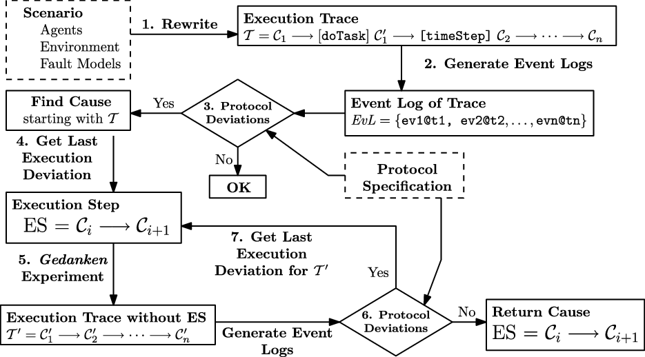
In this section, we introduce the machinery developed to partially automate the detection and diagnosis process. Figure 2 depicts the main steps in the workflow to analyze a soft agents specification. We assume, given as input, the scenario that is the subject of analysis, specified as an initial configuration with agents and environment, the fault models for the sensors, and the protocol specification. The workflow for detecting and diagnosing protocol deviations consists of the following steps:
-
1. We first use Maude’s rewrite engine to construct an execution trace
$\mathcal{T}$
and the associated event log for the protocol language. -
2. Then we extract the event logs from the execution log. This is done by traversing the event log as described in Section 8.1.
-
3. Checking whether the event log satisfies the given protocol specification is done by transforming the problem to an SMT problem and using an SMT-solver. This is described in Section 8.2. If the event log satisfies the protocol, i.e., no deviations are found, then the process can repeat from the beginning with another execution trace.
-
4. Otherwise, we look for the cause of deviation by maximal subprotocols that are satisfiable and find execution deviations at times just after the last events of such maximal subprotocols. Execution deviations are caused by faulty sensors or actions. For example, if it was expected that a faulty speed sensor measured a speed
$s_1$
, but measured a speed
$s_2 \neq s_1$
, then this is an observable execution deviation. This is also described in Section 8.2. -
5. To determine whether the identified execution deviation ES is the cause for the protocol deviation, we carry out a gedanken experiment by rewriting without any faults from the point exactly before ES occurred obtaining a new trace
$\mathcal{T}'$
. -
6. We then extract the event logs of
$\mathcal{T}'$
and check whether it satisfies the protocol. If so, ES is a cause for the protocol deviation. Otherwise, there is another execution deviation happening before ES that is a cause. We repeat by extracting the last execution deviation from
$\mathcal{T}'$
.


Workflow for determining the cause of a protocol deviation. The dashed boxes, scenario and protocol specification are the inputs to the workflow.

We note that the workflow is intended as a tool for exploring effects of different perturbations to determine which cause deviations that should be avoided. It is not complete, but our preliminary experiment indicate that it can be useful.
8.1 Generating execution and event logs
Generating an execution log has two realizations. The first is instrumenting the execution so that the final state contains not only the final system configuration but also a log of the execution. The second is generating a log as a term that can be used as input for other functions, such as checking for deviations. These are different because the result of rewriting is just text that is printed as part of the Maude read-eval-print loop. However, due the Maude’s support for reflection, going from the first to the second is easy as we will see below.
To instrument the execution, recall from Section 4.2.2 that the timeStep rule provides a hook and data structures for log generation, as well as the function updateLog which invokes the model specific function kbLog to compute the configuration component of a log item.
In the BotTeam case study, kbLog collects the agent sensor readings from the environment for the environment part of the log item and collects, for each agent log component, the knowledge items used in deciding actions to propose. This includes location and energy knowledge items and information about targets for treatment and treatment status.
To check satisfaction of a soft agents protocol, we extract an event log from an execution log. Given a log lg, the function flatLog(lg,none,none) returns a pair ekbAll,lkbAll where ekbAll is the union of the environment KBs in the log items of lg and lkbAll is the union of the lkb attributes of each agent in the log items of lg. That is ekbAll is
 $\mathit{EvsA}(\mathtt{lg})$
and lkbAll is
 $\mathit{EvsE}(\mathtt{lg})$
as defined in Section 6.3.
8.2 Protocol deviations
We developed a tool called deviate to detect deviations from a protocol by transforming a protocol plus event log into a logical theory and using the Yices SMT solver to find models of the event partial order component.
To do this deviate first translates the event log into a complete set of atomic and negated atomic formula (clauses), with no free variables, in a finite language over a finite domain. It does this by assuming that if an event does not occur in the log, then the event is in fact false. The protocol is then translated into a simple set of quantifier-free constraints over the theory constructed from the log. The satisfiability of the constraints is then checked by using, the python interface to, the Yices SMT solver. If there is no solution, then we can further investigate the cause by looking at various sub problems. Either by limiting the events in the log to an initial segment or by restricting the form of the constraints generated from the protocol. In this manner, we can further clarify why the initial constraint set has no solution.
We illustrate the information provided by deviate using the following scenario: The initiator bot, b(0), starts at pt(0,1) and the finisher bot, b(1), starts at pt(0,4). The fault model adds location faults for b(1) and the initiator bot waits until b(0) is within 3 moves of the target location to start treatment. Giving deviate the BotTeam protocol and the Environment view of the events from the log for the above scenario we can ask several questions. First, simply, does the event set satisfy the the protocol. deviate reports UNSAT. Next we ask about satisfaction at different levels:
-
— Level 0: Does a mapping
$\sigma$
exist giving times for the specified event patterns? The answer is yes (and a witness is returned). -
— Level 1: Is there a level 0
$\sigma$
that satisfies the local order constraints (LO)? Yes. (
$\sigma$
may be different.). -
— Level 2: Is there a level 1
$\sigma$
that also satisfies the global order constraints (GO)? Yes. (
$\sigma$
may again be different.) -
— Level 3: Is there a level 2
$\sigma$
that also satisfies the event constraints (CS)? NO! (UNSAT) -
— Level 4: Is there a
$\sigma$
that also satisfies the protocol invariants (INV)? NO! (UNSAT)


Finally, the frontier often provides useful information. Intuitively, the frontier specifies a possible minimal stage of concurrent execution where things go wrong, i.e., all earlier stages are consistent with the protocol.
Given a protocol with timelines
 $[tl_0, ... tl_N]$
where each
 $tl_j$
is a sequence of time stamp variables
 $s_{j,k}$
for
 $0 \le k \le N_j$
; and an event log, the problem associated with
 $(i_0, ... i_N)$
is whether there is a mapping of the timeline variables
 $s_{j,k}$
for
 $0 \le k \le i_j)$
that satisfies the protocol restricted to these variables. The frontier is the set of tuples
 $(i_0, ... i_N)$
such that
-
—
$i_j \le N_j$
-
— the problem associated with
$(i_0, ... i_N)$
is UNSAT, -
— the problem associated with any (pointwise) smaller tuple is SAT.


In the case of our example, the frontier has a single element (1,1) and deviate tells us that the unsat core includes [(treatStage (pt 4 0) 4 s11), (treatStage (pt 4 0) 2 s01)]. That is, the finisher bot is late at the first target point.
8.3 Execution deviations
An execution deviation is a result of an agent action that differs from what is predicted by the agent’s model, or a broken sensor reading. In soft agents, an execution deviation can be determined by comparing the local knowledge base of agents and the environment knowledge base. If they differ, it means that there is an execution deviation.
More precisely, an execution deviation (sort EDev) has one of the forms
{ract,lkb,lkb0,ekb0} {ract,lkb,lkb0,{lkb1,ekb0}}
where ract is the (ranked) action executed, lkb is the executing agent’s local KB, lkb0 is the knowledge items updated by the action carried out in lkb0 according to the agent’s model of the world, and ekb0 is the knowledge items in the environment KB, after the action, that disagree with lkb0. In the second case, lkb1 are items in lkb0 that have no corresponding update in the environment KB (for example, if a move action failed, lkb0 will have a location update, but the environment will not). Footnote 7 An execution deviation element (sort EDevsElt) is a time stamped set of execution deviations [t:Time,edevs:EDevSet].
Intuitively, we compute the execution deviations from an execution log by comparing at each step of the log, the local knowledge base of an agent with the expected outcome of performing the same action (without fault models) at that step. Footnote 8 If there is a disagreement, then there is an execution deviation.
Example 8.1. As an example of execution deviations, the following two EDevsElts are obtained from the execution log of the Bot Team scenario with location faults for the finisher bot, b(1). At time 6, the location sensor gave no answer (noLoc), while the environment shows that b(1) is at pt(1,0). No actions were carried out in this step as b(0) is waiting for b(1) to get close enough and b(1) does not know where it is.
[6,{{(zero).RVal,noAct},
(targets(pt(5,4)) @ 2)(target(pt(4,0)) @ 0)
... (energy(b(1),75) @ 6)(mode(b(1),enroute(pt(4, 0))) @ 6),
atloc(b(1), noLoc) @ 6,atloc(b(1), pt(1, 0)) @ 6}]
At time 11 b(1) is trying to charge, since it thinks its at the charging station (pt(3,2)). Thus, it predicts that its energy increases from 55 to 75. However, from the environment perspective (ground truth), we find that the location of b(1) is pt(3,1), charging has no effect, and thus the environment does not record a new value for energy.
[11,{{{cv(100),u(1)},charge(b(1))}, (targets(pt(5, 4)) @ 2) (target(pt(4,0)) @ 0)
... (atloc(b(1), pt(3,2)) @ 11) (energy(b(1), 55) @ 11)
(mode(b(1), enroute(pt(4,0))) @ 11) @ 0, energy(b(1), 75) @ 12,
{energy(b(1), 75) @ 12,(none).KB}}]
8.4 Checking candidate causes
We continue the scenario in Section 8.2 with protocol
 $\mathcal{P}$
, an event log
 $\mathit{EvL}$
from log
 $\mathit{Lg}$
for
 $\mathit{Tr}$
in
 $\mathit{Tr}(iC,\mathit{FM})$
. To check that a candidate event in the log is a possible cause for a deviation in
 $\mathit{Dev}(\mathit{EvL},\mathcal{P})$
we do a gedanken experiment. That is we find a trace
 $\mathit{Tr}'$
in
 $\mathit{Tr}(iC,\mathit{FM})$
that agrees with
 $\mathit{Tr}$
up to the event, avoids the identified event, and continues without further fault injection.
Footnote 9
The idea is inspired by counterfactual reasoning.
ceq gedanken(asys,asysB,n,j) = log1
if log := genLog(asys, ((s n) * 3)) --- 3 rew per time unit
  /\ litem := subLog(log,n,1) --- last trace element
  /\ ekb := getLIEnvKB(litem) --- current environment KB
  /\ aconf := getLIAgents(litem) --- current agent state
  /\ asys1 := updateSys(asysB,s n,ekb,aconf)
  /\ log1 := genLog(asys1,j) . --- hoping for no deviation
asys is the system (with faults) generating
 $\mathit{Tr}$
and asysB contains the base configuration information needed to continue, avoiding the candidate execution deviation. The n is the time just before the candidate execution deviation, and j is how long to continue to check that the protocol deviation is gone. The factor 3 is due to the fact that for every application of the timeStep rule there are two applications of the doTask rule, one for each agent. The 3 is scenario dependent. asys1 augments the logged environment and agent state with knowledge that is constant, such as fence boundary or resource location knowledge, that are not logged, but needed to execute the rules. This information is contained in asysB. The logged environment KB does not contain fault models that are the mechanisms for generating faulty executions, but it may contain obstacles as they are among the entities in the configuration. They must be removed for the gedanken experiment, as they are the other source of perturbations. Note that for the purpose of gedanken the log needs to collect all of the agent state that changes and that is used to decide actions. It also needs to collect all environment knowledge of changing information that is needed for sensor readings or to compute the effects of actions. This may extend what is collected just for determining protocol satisfaction.
The result of this function is a new event log log1 which is then used to check for protocol deviations following the workflow shown in Figure 2. If there are no protocol deviations, then the candidate execution is deemed a possible cause.
Example 8.2. In the case of our BotTeam example with location faults for the finisher bot, b(1), deviation analysis shows that even the first target point has late treatment, and the execution deviations list indicates deviations at times 6, 11, and onward. A gedanken experiment that eliminates faults after time 6,
red gedanken(addFaultsR(mkInitS(pt(4, 0) ; pt(5, 4), true),
 locsf(1), 500),mkInitS(pt(4, 0) ; pt(5, 4), true), 7,90) .
shows that the execution now satisfies the protocol. In particular, we have events
(treatStage(pt(4, 0), 2) @ 11) (treatStage(pt(4, 0), 4) @ 17)
(treatStage(pt(5, 4), 4) @ 35) (treatStage(pt(5, 4), 2) @ 29)
Repeating the gedanken experiment by allowing the fault at 11 but no more we find that the finishing treatment at pt(4,0) is late, but the finishing treatment at pt(5,4) is on time.
(treatStage(pt(4, 0), 2) @ 11) (treatStage(pt(4, 0), 4) @ 28)
(treatStage(pt(5, 4), 2) @ 34) (treatStage(pt(5, 4), 4) @ 43)
9. Experimental Results
In this section, we summarize the results of diagnosis for executions of the BotTeam case study, presented in Section 2, using two and three target locations and a variety of fault models. Our main purpose is not to be comprehensive on the set of experiments, but to illustrate the types of analysis that can be carried out using the proposed machinery and illustrate the different effects of different faults.
9.1 Summary of BotTeam execution results
The scenario for this case study has two bots on a
 $7 \times 6$
grid: b(0), the initiator (class BotI), with sensors locS energyS obstacleS treatS, initially at pt(0,1); and b(1), the finisher (class BotF), with sensors locS energyS obstacleS treatS supplyS, initially at pt(0,4). There is a charging station at pt(3,2) and a supply depot at pt(3,3). Experiments were done for two target lists with initial system configurations initS1a (2 targets) and initS2 (3 targets).
The fault models used in the experiments are described in Tables 1 and 2. The first column of the table is the name used for the fault model in the corresponding experiment summary table. The second column is the knowledge item(s) added to the environment KB specifying the fault. Finally, we also evaluated the impact of the choice of the random sequence used for deciding the occurrence of execution deviations due to the fault models. We specified fault models mvaf1 and mvaf1x with the same fault model specification, but with different subsequences of the sequence generated by Maude. This means that the occurrence of execution deviations using these faults are generally different.
Fault models used in for the experiments involving the 2 target scenario initS1a

Fault models used in for the experiments involving the 3 target scenario initS2

To evaluate the impact of faults on individual sensors, we used fault models for energy, location, movement actuator, and obstacles. We explain in the following the intuition of the fault models in Table 1. The meaning of the faults in Table 2 is similar but using different parameters.
-
— ensfm1 corresponds to the fault model in Example 5.1. In particular, energy measurements may either not return a value or return a value 10 units below the agent’s actual energy. Such wrong measurement may impact the bot’s behavior making them decide to return to the station to recharge.
-
— locsf1x is similar to ensfm1, but considers measurement errors in the location of the bot, instead of the energy.
-
— mvaf1 is similar to the fault model in Example 5.2. In particular, a bot may move erroneously with a probability of 1/5 with an error of pt(-1,0). Moreover, the bot may fail to move altogether with probability of 1/10.
-
— mvaf1x is similar to mvaf1 by using a different random seed.
-
— Obs4-2 is a fault model where there is an unknown obstacle at position pt(4,2).
Tables 3 and 4 summarize, respectively, the results of experiments using the two target scenario, initS1a, and the three target scenario, initS2 with the SA protocol described in Example 6.2. The Faults column names the fault model used (as defined above). The Close column specifies how close the BotI bot requires the BotF bot to be before beginning treatment at a target location. Intuitively, on the one hand, the closer the bots have to be, the less is the risk that the interval between treatments constraints is not satisfied, but on the other hand, the greater is the risk that the overall time of treatment target is not satisfied. For the experiments, the possible values used are 1 and 3 distance units. The PDevs column lists the minimal (with respect to the protocol partial order) protocol deviation(s) if any. The EDevs column gives the number of execution deviations prior to the protocol deviation. In the Gedanken column, a +/- indicates that the gedanken experiment defined by the candidate execution deviation causes confirmed/failed to confirm that elimination of the deviation events eliminated the protocol deviation. na abbreviates “not applicable”.
Summary of experiment results for the 2 target scenario initS1a. If PDevs is none, then EDevs counts deviations in the full execution. Execution deviations due to obstacles are not currently collected. In this experiment, removing the obstacle at event before deviation corrects the behavior

Summary of experiment results for the 3 target scenario initS2

We use the following notation for protocol deviations.
-
— delta(x,y) abbreviates: the log events have
(treatStage(pt(x,y),2) @ t0) (treatStage(pt(x,y),4) @ t1)
-
— with t1 - t0 > = 10 violating the constraint on delay between initial and final treatments.
-
− delta((x0,y0),(x1,y1)) abbreviates: the log events have
(treatStage(pt(x1,y1),2) @ t0) (tloc(b(0),pt(x0,y0)) @ t1)
-
— with t1 - t0 > = 15 violating the constraint on time between target locations.
-
− atloc(b(j),pt(x,y)) indicates an event that was expected by the protocol specification is missing.
From Tables 3 and 4, we see that in all but one case this process was able to identify execution deviations which, when removed, eliminated the protocol deviation. Already from these (non-comprehensive) experiments, it seems that for the scenario with two targets, faults on location and obstacle are most damaging. In contrast, for the scenario with three targets, the impact of energy and movement sensors/actuators start to have a greater impact. This is expected as adding an additional target results in bots needing to traverse greater distances thus consuming more energy and having tighter deadlines.
There is one exceptional case involved in the three target scenario with location sensor faults for BotI. The deviation is an event for which BotF is responsible. The actual problem is that BotF passes through a location adjacent to the target location on the way to the supply depot. It gets stuck there waiting for BotI to finish its treatment because the constraint system gives 0 preference to moving if it is adjacent to its target and BotI is there treating. For the diagnosis system to understand this, more information is needed about the constraints underlying the bots’ action decisions.
10. Related Work
The use of soft constraints and explicit representation of cyber and physical aspects has been discussed in KappÉ et al. (Reference Kappé, Lion, Arbab and Talcott2019) and Talcott et al. (Reference Talcott, Arbab and Yadav2015); Talcott et al. (Reference Talcott, Nigam, Arbab and Kappe2016), Mason et al. (Reference Mason, Nigam, Talcott and Brito2017), respectively. Here we focus on work related to diagnosis.
Comparison with other CPS specification languages: In KappÉ et al. (Reference Kappé, Lion, Arbab and Talcott2019), an automaton-based formalism for compositional design was developed along with an extension of Linear Temporal Logic with two unary connectives that reflect the compositional structure of actions. A method was developed to use the logic and an algebra of action preferences to diagnose undesired behavior by tracing the falsification of a specification back to one or more culpable components. Instead of using temporal logics, we propose a protocol specification which is a domain-specific specification language for mission requirements. A key advantage of this specification language is that it is similar to the operations related to the planning problems that are considered for mission accomplishment for CPS. This domain-specific aspect of protocol specification improves, arguably, the understanding of requirements to CPS engineers. It remains open, although likely, to translate these specifications into fragments of suitable quantitative temporal logic formulas.
The soft agents CPS model is complimentary to the work on hybrid systems (Mitra Reference Mitra2021). It abstracts from details at the level of differential equations and device controllers to focus on short term adaptive planning. Issues that are similar in spirit arise at multiple levels. Reachability analysis is an important tool in both cases, but may be concerned with different properties.
Falsification is an important topic in hybrid systems research (Frehse and Althoff Reference Frehse and Althoff2021). In falsification, the problem is to develop efficient methods for finding inputs that drive a system to a bad state. Falsification is also relevant in security protocol analysis, where falsification means finding an attack that leads to violation of a security property (Basin et al. Reference Basin, Cremers and Meier2012, Reference Basin, Cremers, Dreier and Sasse2017; Schmidt et al. Reference Schmidt, Meier, Cremers and Basin2012). The detection and diagnosis problem studied in the current paper is concerned with determining which environmental perturbations such as faulty sensors or actuators or obstacles cause protocol violations. The use of attack models (how an intruder can manipulate messages or emulate honest participants) in security protocol analysis is analagous to the use of fault models in our work, in the sense that it used to identify threats/perturbations which which cause a system to fail to satisfy given properties. In Basin et al. (Reference Basin, Cremers and Meier2012), the form of attacks found for different properties is used to (manually) identify “root” causes and suggest repairs. In Schmidt et al. (Reference Schmidt, Meier, Cremers and Basin2012), constraint solving is used to verify/falsify protocols.
Comparison with related Counter-Factual Work: Our use of ‘gedanken experiments’ was motivated by Gössler and Stefani (Reference Gössler and Stefani2016, Reference Gössler and Stefani2020), Laurent et al. (Reference Laurent, Yang and Fontana2018). A general semantic framework for fault ascription is proposed in Gössler and Stefani (Reference Gössler and Stefani2016) based on counterfactual analysis to identify necessary and sufficient causes of faults in component-based systems. The key is an operation CF(X,L) that constructs from a log L and candidate violations X, a set of counterfactual configurations modeling system behavior “if X had not happened”, and there are no new component failures. This work is extended and refined in Gössler and Stefani (Reference Gössler and Stefani2020) including new requirements and properties for the counterfactual construction operator and a concrete example. In Gössler and Stefani (Reference Gössler and Stefani2020), hyperproperties are also considered, which is an interesting direction for future work.
GS (Gössler and Stefani Reference Gössler and Stefani2020) compare counter-factual reasoning to the mathematical definition of causality proposed by Pearl and Halpern (PH) (Halpern 2005; Pearl Reference Pearl2000) PH models are deterministic while CPS systems are distributed, nondeterministic systems. PH causes are observable, while GS ascription may propose unobserved causes. In the PH formalism, there is no notion of specification or fault in causality.
A symbolic approach to fault ascription in real-time systems based on timed automata is presented in Gössler and Astefanoaei (Reference Gössler and Astefanoaei2014). Here an execution trace violating a safety property is analyzed by counterfactual reasoning which is reduced to a model-checking problem.
Laurent et al. (Reference Laurent, Yang and Fontana2018) defines the semantics of counterfactual analysis for traces of events of stochastic rule-based models. The objective is to construct a causal diagram that explains how a phenomenon of interest occurred, given a trace of a system behavior. The semantics is based on sampling counterfactual trajectories that are probabilistically as close to the factual trace as a given intervention permits them to be.
Comparing Gössler and Stefani (Reference Gössler and Stefani2020) (GS), Laurent et al. (Reference Laurent, Yang and Fontana2018) (LF), and the current work (SA), we note that the intended contexts of use are somewhat different: SA is focused on design time, and GS seems to be focused on run time analysis. GS and SA aim to find causes of faulty behavior in software/CPS, while LF is using causal analysis to understand mechanisms of natural (biological) processes. SA and LF use rule-based component specifications and trace semantics (LF traces are stochastic simulations), while GS uses configuration structures to describe components and systems with added (faulty) behaviors. SA uses explicit fault models to add faulty behavior to systems. GS properties are configuration structures, while SA properties are specified by protocols. In GS logs not all events are observable, while SA logs contain all the events relevant to the protocol specification, reflecting a difference between design time and runtime analysis. GS proposes counterfactual constructors to generate all behaviors consistent with a given log where given violations no longer happen. SA provides mechanisms to identify potential causes of violations and a mechanism to check by generating traces avoiding the candidates. The LF approach additionally provides a means for measuring distance of the counter factual traces from the original. An interesting direction of future work is to recast some of the GS requirements for counterfactual constructors in the SA setting. Another interesting direction for developing the SA approach is to consider distributed detection and diagnosis at runtime, which will entail some events being unobservable.
There are many protocols for carrying out diagnosis. For example. protocols are used in Debouk et al. (Reference Debouk, Lafortune and Teneketzis2000) as a mechanism to define diagnosers for distributed event systems. Here each component does local diagnosis and reports to a central coordinator component that carries out system-level diagnosis. A protocol specifies the communication and system-level decision rules. To the best of our knowledge, the use of protocols to specify behavior whose deviations are to be diagnosed in the context of CPS seems new.
11. Conclusions
This paper presents a formal framework enabling the diagnosis of cause for deviations from desired behavior to support design time decisions. Our formal framework extends the soft agents framework which is implemented in Maude. In particular, we extend Soft Agents with fault models, define a protocol specification language, from which protocol deviations are defined. We then propose a workflow for determining causes for deviations. This workflow is partially automated by using Maude and an SMT-solver. We demonstrate the workflow with some experiments involving a proof of concept BotTeam scenario.
There are several directions that we are currently investigating. The first is on the expressiveness of the protocol language. We suspect that the proposed workflow can be extended to support further protocol constructs, such as finite branching and finite unfolding. We are also considering other forms of constraints involving other than time variables such as resources, following our previous work on protocol security (Urquiza et al. Reference Urquiza, Alturki, Kirigin, Kanovich, Nigam, Scedrov and Talcott2021). We have developed and tested the ideas using simple, easy to understand examples. An important future direction is developing methods to scale to more complex systems. There are several approaches to investigate including reducing interleaving by replacing some rewrite rules by equations, using symbolic rewriting where configurations are pairs consisting of a term with variables and a boolean condition constraining the variables (Lee et al. Reference Lee, Kim, Bae and Ölveczky2021; Nigam and Talcott Reference Nigam and Talcott2022) and leveraging modularity. Finally, we are also investigating further scenarios, such as scenarios involving autonomous vehicles.
Acknowledgments
Kim and Mason were partially supported by the US Office of Naval Research under award number N00014-15-1-2202. Talcott was partially supported by the US Office of Naval Research under award numbers N00014-15-1-2202 and N00014-20-1-2644. Nigam was partially by CNPq grant 303909/2018-8.