




No CrossRef data available.
Article contents
- Abstract
- INTRODUCTION – THE IMPACT OF TICK ECOLOGY ON PATHOGEN TRANSMISSION DYNAMICS
- PHYSIOLOGICAL ECOLOGY – THE ADAPTATION OF TICKS TO THEIR NATURAL ENVIRONMENT
- POPULATION ECOLOGY: CONSEQUENCES OF DEMOGRAPHIC PROCESSES
- ECOLOGICAL AND EPIDEMIOLOGICAL CONSEQUENCES OF TICK–HOST INTERACTIONS
- PREDICTIVE MAPPING OF THE RISK FACTORS OF TICKS AS VECTORS
- CONCLUSIONS
- ACKNOWLEDGEMENTS
- References
Tick ecology: processes and patterns behind the epidemiological risk posed by ixodid ticks as vectors
Published online by Cambridge University Press: 19 April 2005
Article contents
- Abstract
- INTRODUCTION – THE IMPACT OF TICK ECOLOGY ON PATHOGEN TRANSMISSION DYNAMICS
- PHYSIOLOGICAL ECOLOGY – THE ADAPTATION OF TICKS TO THEIR NATURAL ENVIRONMENT
- POPULATION ECOLOGY: CONSEQUENCES OF DEMOGRAPHIC PROCESSES
- ECOLOGICAL AND EPIDEMIOLOGICAL CONSEQUENCES OF TICK–HOST INTERACTIONS
- PREDICTIVE MAPPING OF THE RISK FACTORS OF TICKS AS VECTORS
- CONCLUSIONS
- ACKNOWLEDGEMENTS
- References
Abstract
The population ecology of ticks is fundamental to the spatial and temporal variation in the risk of infection by tick-borne pathogens. Tick population dynamics can only be fully understood by quantifying the rates of the demographic processes, which are influenced by both abiotic (climatic) factors acting on the free-living tick stages and biotic (host) responses to the tick as a parasite. Within the framework of a population model, I review methods and results of attempts to quantify (1) rates of tick development and the probability of diapause, (2) the probability of questing for hosts by unfed ticks, (3) the probability of ticks attaching to a host, and (4) tick mortality rates. Biologically, these processes involve the physiological and behavioural response of ticks to temperature, moisture stress and day length that result in specific patterns of seasonal population dynamics and host relationships. Temperate and tropical patterns will be illustrated with reference mostly to Ixodes ricinus and Rhipicephalus appendiculatus, respectively.
Information
- Type
- Research Article
- Information
- Copyright
- © 2004 Cambridge University Press
INTRODUCTION – THE IMPACT OF TICK ECOLOGY ON PATHOGEN TRANSMISSION DYNAMICS
The ecology of ticks, the outcome of their interactions with their natural environment, is fundamental to the spatial and temporal variation in the risk of infection by tick-borne pathogens. Due to the biology of ticks as blood-feeding parasites, their physical environment includes the host itself. This biotic environment reacts to the tick's presence in both the short and the long term in ways that the abiotic environment cannot do, imposing physiological, population and evolutionary pressures on ticks. Ticks, however, are only intermittent parasites, spending the majority of their life cycle free within their habitat where they are at the mercy of abiotic factors such as habitat structure and climate. They take only one (ixodid ticks) or a few (argasid ticks) very large blood meals per life stage, as larvae, nymphs and adults, then develop to the next stage, which takes weeks, months or even years, depending on the ambient temperature. This inter-stadial period is usually passed off-host, although the relatively few two- and one-host ticks (e.g. Hyalomma anatolicum excavatum and Boophilus microplus, respectively) remain on the host for one or both of the inter-stadial periods. For simplicity, and because generally less is known about the ecology of argasid ticks, what follows will refer almost exclusively to ixodid ticks.
At the individual level, a tick's potential as a vector is enhanced by its habit of taking such large, slow blood meals, and by its adaptations to survive the host's defences (see chapter by Brossard & Wikel in this Supplement). At the population level, vector potential is severely constrained by the limitations of taking such few meals. Vector–host contact rates can never exceed three per generation, and are reduced to only one per generation for one-host species that take all three meals on the same individual host. Furthermore, a tick of one stage that acquires pathogens in its blood meal from an infected host cannot transmit them to a new susceptible host until it feeds again as the next stage. Trans-stadial maintenance of infection (of which trans-ovarial transmission, from female to larvae, is a special form), is the sine qua non of an ixodid tick's performance as a vector. Furthermore, the transmission cycle must involve at least two tick stages feeding on the same host individual (although not necessarily at the same time), one to transmit and the preceding stage to acquire. (Exceptions involve transmission by peripatetic male ticks of some species, either directly by their taking small meals on more than one host, or via the venereal route – Alekseev et al. 1999.) This introduces a very long delay into the transmission process, accompanied by high tick mortality, both of which vary geographically and seasonally with climate. Climate-driven tick seasonal population dynamics therefore have an impact on the pace and force of transmission (the longer the delay in transmission, the slower the transmission cycle and the fewer ticks survive). Population dynamics also determine the seasonal abundance of active ticks questing for hosts and therefore the risk of infection.
In the case of some pathogens, the very existence of the specific transmission route also depends on a particular pattern of the vector's seasonal dynamics. Tick-borne encephalitis (TBE) virus (see chapter by Labuda & Nuttall in this Supplement), for example, is very short-lived in its principal rodent hosts, and commonly does not develop patent systemic infections (Labuda et al. 1993a,b, 1996), so it must be transmitted directly from infected nymphal Ixodes ticks to uninfected larvae co-feeding on the same hosts. Only where large numbers of larvae feed together with nymphs, determined both by climate and host factors as described below, is there sufficient transmission to allow TBE virus to persist (Randolph et al. 1999). For this, larvae and nymphs must have synchronous seasons of activity, which is characteristically seen within TBE foci, but not elsewhere (Randolph et al. 2000). This synchrony may occur at any time of the year (see Figs. 1–4 in Randolph et al. 2000), but will be most significant epidemiologically in the spring and summer when both tick stages are most abundant. This is also when most human TBE cases occur (Zabicka, 1994; Danielová et al. 2002). Larval–nymphal synchrony and TBE foci are statistically significantly associated with a particular seasonal land surface temperature profile, characterized by a relatively rapid rate of cooling during the autumn (Randolph et al. 2000). These empirical conclusions have been disputed on the grounds that TBE virus can also be transmitted from transovarially infected larvae to other co-feeding larvae (Danielová et al. 2002). This transmission route cannot, however, account quantitatively for persistent cycles of TBE virus (see below), nor explain the absence of TBE in many places where Ixodes ricinus is abundant (Randolph et al. 2000).
This system is just one example of a dominant theme of this chapter – the general influence of climate on tick–host–pathogen relationships and therefore on the epidemiology of tick-borne diseases. It also highlights another theme – that ecological (or epidemiological) systems can only be fully understood by quantifying the rates of the constituent processes. Differential rates and epidemiological patterns depend on specific biological features of pathogens, vectors and hosts. The longer the duration of infectivity of the pathogen in the vertebrate host, for example, the greater the window of opportunity for transmission and so the less specific is the pattern of tick seasonal dynamics necessary for persistent enzootic cycles. Borrelia burgdorferi sensu lato, the agent of Lyme borreliosis (see chapter by Piesman & Gern in this Supplement), survives in vertebrates for many weeks or months. Consequently, it is much more wide-spread, with higher infection prevalences, than TBE virus, despite being transmitted by the same vector species.
The ultimate aim of attempts to describe and explain any system must be to make testable predictions, ideally within the quantitative framework of a model. A tick population model can predict all the major risk factors for tick-borne diseases, the distribution (i.e. places where tick populations survive), abundance, seasonal dynamics and even host relationships of the vector tick. Ticks, however, pose a considerable challenge to population modellers. To be of any epidemiological use, the model must predict the abundance of three overlapping life stages simultaneously. This complexity must be captured in the simplest possible terms by focussing on the following four essential processes (Fig. 1). First there is entry into the population of unfed ticks of each stage by development from the previous stage. Secondly, there is a certain probability that an unfed tick will quest actively for a host on any day. These two terms describe the input into the questing tick population. Thirdly, if a tick is questing, it has a daily probability of attachment to a host. This will vary with host species and density, and so offers some insight into host relationships. Finally, there are daily rates of mortality, which are specific to each stage and state (questing, feeding and engorged). These latter two are output terms. Only analysis of field observational and experimental data can yield reliable measures of the quantitative relationships between these processes and the abiotic and biotic predictor variables.

Fig. 1. The structure of a population model for the tick Ixodes riciuns. Factors which determine the rates of the processes described within each box may be abiotic (solid arrow) or biotic (dotted arrow).
Within this framework, the following review will examine how both the biotic and abiotic elements of the tick's environment give rise to the precise patterns of tick distribution, seasonal abundance and host relationships that determine pathogen transmission dynamics and therefore spatial and temporal variation in the risk of infection. This review does not aim to be exhaustive. Instead, I shall focus on studies that illustrate the hierarchy of processes and patterns inherent in the epidemiological risk posed by ticks as vectors. At the base is the physiological ecology of ticks, the adaptation of individuals to their natural habitats. As each tick is born, lives and dies, it contributes to the overall rates of the demographic processes that add up to the next level, population ecology. In this chapter I shall deal with tick–host relationships as properties of populations, rather than at the individual level as described in previous chapters. Finally, I shall review recent attempts to describe and explain wide-scale patterns of epidemiological risk factors as a way towards biological, process-based predictive risk mapping. Most of the detailed accounts will use I. ricinus as a temperate exemplar and Rhipicephalus appendiculatus as a tropical exemplar, drawing on my first-hand experience of primary research on these species.
PHYSIOLOGICAL ECOLOGY – THE ADAPTATION OF TICKS TO THEIR NATURAL ENVIRONMENT
Natural outcomes of temperature-dependent development rates
Entry into a population is measured by the birth rate (and immigration rate where appropriate). Because a female ixodid tick lays a single large egg mass (typically several thousand eggs) over a short time period, a more useful demographic input parameter is the development rate from one stage to the next. In common with most physiological processes in poikilothermic animals, inter-stadial development rates of ticks increase non-linearly with increasing ambient temperature. To be of most use in predicting development periods under varying temperature conditions in different parts of a tick species' range, temperature-dependent development rates should be established under constant conditions in the laboratory. In equatorial regions with minimal seasonal temperature variation, however, field observations may be sufficiently precise.
The daily rates for both the tropical tick R. appendiculatus and the temperate species I. ricinus (Campbell, 1948) may be adequately described by second-order polynomial relationships with temperature (R2 values range from 0·924 to 0·998), but there appear to be considerable differences in the precise rates for each species and each stage (the latter more marked for R. appendiculatus than I. ricinus) (Fig. 2). In Slovakia, a sympatric tick species, Dermacentor reticulatus, develops very much more rapidly than I. ricinus in the same habitat, for example passing from engorged larva to moulted nymphs within one month during the summer rather than two or three. These differences suggest an element of adaptation evolved by each species, which may extend to each geographical strain of the same species. It is essential, therefore, to establish the correct rates for each species, laborious though this is. Quantitative inter-stadial linkages cannot be deduced reliably by assuming that development periods correspond to the interval between peak numbers of ticks seen questing in the field (see Figs. 4 and 5 below). In this and other ways, Randolph (1993) stands as an object lesson of what not to do!

Fig. 2. The relationships between temperature and daily rates of inter-stadial development. Note the same pattern, but quantitative differences between stages (circles, larva–nymph; squares, nymph–adult; triangles, female–larva), and between species (filled symbols, Rhipicephalus appendiculatus; open symbols, Ixodes ricinus). Re-drawn from original data in Campbell, 1948; Branagan, 1973; Kaiser et al. 1988.
Using a day-degree summation method, natural development periods in the field may be estimated by applying daily development rates to varying temperatures within the tick's habitat. Development is complete once the proportional development per day sums to 1, after which there is a period of ‘hardening off’ before the emergent tick starts to quest. Because it is so important to describe this foundation layer of the tick's population performance accurately, temperature should be measured as closely as possible to the micro-habitat in which the tick undergoes its development. Soil surface temperatures are buffered both diurnally and seasonally compared with air temperature, so the use of uncorrected air temperatures as predictors of development rates gives a highly inaccurate picture. In southern UK, for example, air temperature measured 50 cm above the ground predicts 10–40% faster development by I. ricinus larvae for most of the spring and summer months (Fig. 3), resulting in the emergence of nymphs 2–3 weeks earlier. Such inaccuracies could have a marked knock-on effect on the predicted phenology of tick populations, especially in continental Europe where air temperatures are even more variable. Only when we know precisely which ticks, and therefore how many, of one stage give rise to which and how many ticks of the next stage, counted in the field, can we progress to further analysis of the seasonal population dynamics of the tick and transmission dynamics of any pathogens.

Fig. 3. Seasonal and geographical variation in daily rates of larva–nymph inter-stadial development rates predicted by day-degree summation models based on ambient temperatures. Squares, Ixodes ricinus in Dorset, UK ([squf ]) and Wales, UK (□); circles, Rhipicephalus appendiculatus in Kirundo, Burundi ([bull ]) and Gulu, South Africa (○). The grey symbols () show the effect of basing the predictions for Dorset on air, rather than soil, temperatures.
The simple fact of geographical variation in absolute ambient temperatures and their seasonal variability results in contrasting patterns of recruitment to questing tick populations, potentially continuous in the tropics and even in the sub-tropical regions of South Africa (Randolph, 1997), but intermittent in temperate regions. Where development rates drop very low and even to zero for large parts of the year (Fig. 3), development periods are telescoped and so emergence of unfed ticks becomes more synchronised.
Diapause – significance in tropical and temperate tick-borne disease systems
‘Behavioural’ diapause in tropical ticks
As an adaptation to ensure that emergence coincides with optimal conditions for survival, many tick species have incorporated some form of diapause into their life cycles. In southern Africa, for example, recruitment of R. appendiculatus is not in fact continuous throughout the year (Rechav, 1981, 1982; Short & Norval, 1981; Pegram & Banda, 1990; Randolph, 1997). This species illustrates nicely the plastic, presumably adaptive nature of diapause. Diapause is confined to unfed adult ticks, which do not always quest and feed as soon as they have hardened after emergence from the engorged nymphal stage. In South Africa, those which emerge after July each year do not start questing until some time after November of the same year (Rechav, 1981; Randolph, 1997). This diapause appears to be induced by short day lengths (the southern winter solstice occurs in June) (Rechav, 1981; Short & Norval, 1981; Pegram & Banda, 1990; Madder et al. 1999). As a result, there are periods of near absence of each tick stage sequentially during the year (Fig. 4a), and the majority of the vulnerable egg-to-larval stage occurs during the warm wet season (December–May), which would favour rapid development and good survival, although excessively wet conditions are correlated with increased mortality (see below).

Fig. 4. Seasonal variation in the number of larval, nymphal and adult Rhipicephalus appendiculatus at (a) Gulu, South Africa (data from Rechav, 1982) and (b) Kirundo, Burundi (data from Kaiser et al. 1988). The grey arrows indicate which ticks of one life stage gave rise to which ticks of the next stage (according to Randolph, 1994a, 1997). In (a), ‘d’ marks the months of diapausing adults, and asterisks mark those adults and larvae which were counted after recruitment had apparently ceased (see text).
In contrast, in equatorial Africa, where long cold dry seasons do not occur, the same tick species does not show any diapause (Branagan, 1973). All tick stages feed throughout the year (Newson, 1978; Kaiser, Sutherst & Bourne, 1982, 1991; Kaiser et al. 1988), resulting in continuous overlapping generations each of c. 8–9 months duration (Fig. 4b). Marked declines in abundance of all stages occur simultaneously during the dry season. Based on laboratory experiments, Madder et al. (1999) concluded that there is a latitudinal gradient in the propensity to diapause, with ticks from Zimbabwe exhibiting diapause more consistently than those from Zambia. While long day length may trigger diapause termination in the south, further north in Zambia diapause may end gradually over periods of up to five months, perhaps in response to physiological ageing (Berkvens, Pegram & Brandt, 1995).
This variable pattern of diapause is significant not only for the survival of tick populations, but also for the epidemiology of associated infections. Norval et al. (1991) concluded that the occurrence of diapause in R. appendiculatus in southern Africa may account for the absence there of the virulent strain of Theileria parva that causes East Coast Fever in cattle in eastern and central Africa (see chapter by Bishop et al. in this Supplement). Only where there is sufficient overlap between the more or less continuous activity periods of the different tick stages can the virulent strain of T. parva be acquired from infected cattle by larvae and nymphs and transmitted onwards by nymphs and adults. If this is true, it suggests that inter-stadial transmission from larvae to nymphs, which do in fact overlap considerably more than nymphs and adults in South Africa (Fig. 4a), may not be sufficient to maintain cycles of virulent T. parva. The larval–nymphal route was indeed shown experimentally to be less efficient than the nymphal–adult route (Ochanda et al. 1996). The less virulent strain of T. parva that causes January or Corridor disease survives for longer periods in carrier cattle, and so can be acquired by nymphs and transmitted by adults where there is less inter-stadial overlap; hence its occurrence in southern Africa.
‘Morphogenetic’ and ‘behavioural’ diapause in temperate ticks
Temperate tick species have to deal with even more marked seasonality in environmental conditions. The inter-stadial periods between two or more stages of Ixodes species, including I. rubicundus from South Africa (Fourie, Belozerov & Needham, 2001), may be prolonged (i.e. adjusted) by a variable delay in the onset of development (Campbell, 1948; Kemp, 1968), commonly called ‘morphogenetic diapause’ (Belozerov, 1982). As this occurs in I. ricinus that are collected from the field after July, fed in the laboratory and then held in either constant laboratory conditions (Campbell, 1948; Kemp, 1968) or quasi-natural field conditions (Chmela, 1969; Cerny, Daniel & Rosicky, 1974; Daniel et al. 1976, 1977; Gray, 1982), diapause must be triggered by conditions experienced by the questing stages, or the difference between pre- and post-engorgement conditions. Belozerov identified photoperiod as the major cue for diapause, specifically the change from long (pre-feed) to short (post-feed) day length for both Palaearctic (I. ricinus and I. persulcatus) and Nearctic (I. scapularis) members of this species complex (Belozerov, 1998a; Belozerov & Naumov, 2001).
The exact light sensitivity of the photoreceptor cells on the dorso-lateral surface of all stages of I. ricinus (Perret et al. 2003) is unknown, but ticks have now been shown to respond to simulated natural changes in day length (Beattie & Randolph, unpublished observations), which are much more gradual (c. 20–30 minutes per week) than those used in Belozerov's experiments (typically an 8-hour difference within a few days, either side of feeding). Under natural conditions there is a latitudinal gradient in the date of diapause onset. It occurs in I. ricinus that feed from the end of July onwards in Scotland (c. 56° N), from mid-August in Ireland (c. 53° N) and from the end of August in the Czech Republic (c. 49° N). At this time of year, day length is longer but declines faster with increasing latitude, suggesting that the rate of day length change may be a critical cue. However, in light conditions that simulated rapid or slow day length decrease equivalent to July–October at St Petersburg (60° N) and Valtice in the Czech Republic (49° N), respectively, and under 18 °C constant temperature conditions, ticks entered diapause as photoperiods reached the same absolute length, c. 13 hours light, irrespective of the rate of decrease (Beattie & Randolph, unpublished observations). Therefore other factors, such as decreasing temperature, or even increasing age of the tick, both of which are known to enhance the diapause response (Belozerov, 1967, 1970; Fourie et al. 2001), may be responsible for its earlier onset further north, although on their own they would offer less reliable signals to ticks.
There is clearer evidence that temperature is instrumental in breaking morphogenetic diapause in I. ricinus. Ticks exposed to even a brief period of 0 °C show non-delayed development, similar to those fed in the spring (i.e. pre-July) (Campbell, 1948). This ensures that all ticks, whenever they feed after July/August, start development once temperatures increase after the winter (Fig. 3). Those which feed before July develop rapidly without delay. Under a wide range of conditions across the UK, the combination of diapause and seasonal temperature-dependent development rates acts to synchronise the emergence of virtually all unfed ticks of each stage to within a couple of months every autumn (Randolph et al. 2002). This conclusion was validated by examining the physiological state of questing ticks; emergence dates predicted from the day-degree summation development model (Fig. 5) coincided exactly with the first appearance in the field of questing nymphal and adult ticks with high fat content.

Fig. 5. Seasonal variation in the number of larval, nymphal and adult Ixodes ricinus in Dorset, UK. The arrows indicate which ticks of one life stage gave rise to which ticks of the next stage (according to Randolph et al. 2002). Asterisks mark show dates of first appearance of high-fat (newly recruited) nymphs and adults in the field.
Fat is a source of energy derived from each blood meal, that can be used as a marker of physiological ageing in the field (Uspensky, 1995; Walker, 2001). After emergence, fat is used to fuel a tick's locomotory and physiological activity involved in locating and ascending vegetation stems from which to quest, and descending to moist conditions at the base of the vegetation to restore its fluid content by passive and active uptake of atmospheric water (Knulle & Rudolph, 1982; Needham & Teel, 1991; Sonenshine, 1991; see chapter by Bowman & Sauer in this Supplement). Its natural rate of usage therefore varies with seasonal activity and climatic conditions (Steele & Randolph, 1985; Randolph & Storey, 1999), allowing a distinction between the calendar age and physiological age of ticks. At three field sites in the UK, at the end of the summer all nymphs and adults of I. ricinus had very low fat content until, in September or October, a large proportion of ticks had distinctly higher fat content, typically about three times as much when corrected for tick size (Randolph et al. 2002). At this point two overlapping cohorts of ticks were clearly present (Fig. 6). Thereafter modal fat content decreased throughout the following spring. Increasing numbers of ticks became active in the spring, but they had lower fat content than ticks seen in the previous autumn, indicating that they had endured a longer interval between emergence and questing than had the new recruits in the autumn. Through the summer, fat was gradually exhausted by ticks still questing for hosts, so that virtually no low-fat ticks persisted beyond October.
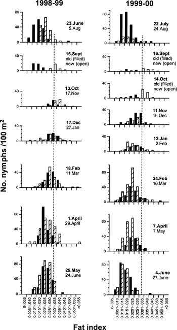
Fig. 6. Seasonal changes in absolute frequency distributions of questing nymphal Ixodes ricinus with different fat content indices counted per 100 m2 in Dorset, UK, starting with late summer at the top in each of two years. Data for two monthly samples are presented in each histogram, showing the earlier data of each pair as filled bars and the later date hatched. In September/October when old and new recruits occur within the same sample, new recruits are shown by open bars. The vertical dotted line is purely to guide the eye.
So it appears that under a wide range of climatic conditions in the UK, a single cohort of each stage of I. ricinus is recruited each year in the autumn and then survives for one year until the ticks have either fed or died of fat exhaustion. The same appears to be true for I. persulcatus, despite a prolonged total life cycle (up to six years) in more extreme climates (Filippova, 1985; Uspensky, 1995; Korenberg, 2000). This timing of recruitment does not, however, coincide with the timing of peak numbers of ticks seen questing in the field. Most newly emergent ticks delay their questing activity until the following spring in many parts of Europe, inter alia (Lees & Milne, 1951; Daniel et al. 1976; Gray, 1985; Randolph et al. 2002). This may be true ‘behavioural diapause’ (Belozerov, 1982), similar to that seen in adult R. appendiculatus and I. pacificus (Padgett & Lane, 2001), although the triggers will be species-specific. Belozerov (1982) concluded that unfed stages of I. ricinus entered diapause in response to short day length. In the field in mild climates, however, ticks may be active from January onwards (Fig. 7), suggesting that decreasing day length beyond a certain level, rather than absolute day length, may be the cue for diapause. Ticks also vary their questing activity in response to their immediate climatic conditions (see below). All-in-all, the pattern of seasonal questing by ticks that diapause in the unfed stage is the product of behaviour (and mortality) superimposed on the phenology. It is time to move to the second box of the tick population model (Fig. 1) and consider determinants of the probability of questing.

Fig. 7. Seasonal variation in maximum air temperature (Ta) and numbers of questing larval (○) and nymphal ([bull ]) Ixodes ricinus at three sites in the UK (note that larval density is presented at 33% of observed level). Dotted and dashed lines indicate the temperature thresholds for the onset of seasonal activity of larvae and nymphs, respectively.
Environmental constraints on host-questing activity and behaviour
Temperature and day length
Abiotic factors impose constraints on when, where and how ticks quest for hosts. Interacting with the putative inhibitory effects of decreasing day length, and the supposed converse permissive effects of increasing day length, low winter temperatures in temperate regions inhibit tick activity. Mild winters in southern UK allow us to disentangle day length and temperature as determinants of tick questing probability. In contrast to the north of the UK, Switzerland and Wales, where questing activity by nymphs and adults of I. ricinus does not begin in the spring until the weekly mean maximum temperature has reached 7 °C (Macleod, 1936; Perret et al. 2000; and Fig. 7c, respectively), in the south of the UK from 1998 to 2000 winter temperatures did not drop low enough to inhibit nymphal and adult questing activity (Fig. 7a, b). In the south, however, fewer questing nymphs (and adults – data not shown) were counted from October to December, when temperatures were well above threshold levels, than from January onwards. Thus we can propose that at the end of each year, decreasing day length reduces the probability of questing and low temperatures may inhibit activity altogether (see Wales, Fig. 7c), while at the start of each year, increasing day length is permissive, but only if temperatures are high enough. Gradual recruitment to the questing population will occur as temperatures reach this critical level in increasing parts of the ticks’ over-wintering micro-habitats (Eisen, Eisen & Lane, 2002). Because the use of field sampling data to impute questing activity may, however, be confounded by variable rates of disappearance from the questing population through variable feeding and/or mortality rates (see below), experiments under controlled conditions are essential to test this proposed explanation.
Tick size
Activity threshold temperatures vary inter-specifically, inter-stadially, and even intra-stadially, which appears to be size-dependent (Clark, 1995). In the UK, the onset of larval activity coincides with a threshold of 10 °C, rather than 7 °C, mean maximum temperature (Fig. 7). Furthermore, at our UK sampling sites, smaller nymphs (and adults – not shown) started questing later each year (Randolph et al. 2002). Each new cohort of ticks that appeared on the vegetation in the autumn showed a normal size (fat-free weight) distribution, virtually symmetrical about a median of 75–85 μg, which then changed seasonally (Fig. 8). A sub-set of larger nymphs started questing in February, with only 15–30% <80 μg and almost none <60 μg. As the year progressed, the questing population was composed increasingly of smaller nymphs, as small ticks appeared from March onwards.

Fig. 8. Seasonal changes in the size (i.e. fat free weight) composition of populations of questing nymphal Ixodes ricinus during the life-span of a single cohort on Exmoor, UK 1998–1999. Sample dates and sizes are shown in the key. With permission from Randolph et al. 2002.
Figure 8 also shows that once recruitment has ceased beyond April/May and tick numbers fall, the largest ticks (>100 μg) disappear first and only the smallest ones persist to September. Larger ticks arrive sooner and may find hosts more rapidly if their relatively higher energy levels (Van Es, Hillerton & Gettinby, 1998; Randolph et al. 2002) permit them to quest for longer periods. Smaller ticks (including all larvae – Fig. 7) that arrive later may find hosts more slowly if they are forced into temporary inactivity during the summer by the other major constraint of questing probability, moisture stress.
Moisture stress
Despite generic adaptations permitting them to inhabit dry environments, water loss remains the Achilles heel of all terrestrial arthropods, including ticks. Ticks that live in xeric habitats show special adaptations. They tend to be larger than average, thereby reducing their relative surface area, but still they must shelter in cracks and under stones. They cannot sit in the open and ambush passing hosts, but must hunt them actively, travelling fast from shelter to host when the opportunity arises. Sonenshine (1991) describes how ‘camel ticks, Hyalomma dromedarii, emerge from the barren sand around desert caravansaries and run across the hot, exposed ground to attack people and livestock when these hosts were resting near their shelters’.
Other tick species live in far less challenging habitats, but have lower tolerance to water stress. They can sit on vegetation to await passing hosts, but must still limit their host-questing activity to maintain their water balance. Questing behaviour therefore varies diurnally and seasonally with climate (Lees & Milne, 1951; Belozerov, 1982). Triggered by the onset of darkness, ticks appear to make use of moist night-time conditions to walk, thought to be related to selecting suitable questing locations (Perret et al. 2003). In experimental conditions, nymphs walked further after periods of quiescence (median 43 cm, max 9·7 m) than after questing (median 17 cm, max 2·9 m), while those denied atmospheric moisture walked between 5 and 31 m until they died.
Under favourable conditions, ticks may remain in questing positions on the vegetation for periods of several days (Lees & Milne, 1951; Loye & Lane, 1988), but they descend much more frequently in response to increased saturation deficit (SD – a measure of the drying power of the atmosphere that depends on both temperature and relative humidity – RH) so that, commonly, fewest ticks quest during the middle of the day. Macleod (1935) observed that I. ricinus demonstrates positive geotropism at saturation deficits above 4·4 mm Hg (equal to 80% RH at 24 °C, or 71% RH at 18 °C). In the field, reductions in the questing I. ricinus population coincided with maximum SD above 4·4 mm Hg (Perret et al. 2000), with adults less affected than nymphs. Likewise, experiments in quasi-natural arenas (Randolph & Storey, 1999) revealed that under such dry conditions questing activity was diminished more amongst larvae than nymphs, but for both stages it was reversible once moist conditions were restored, i.e. high SD, even up to 15–20 mm Hg, induced quiescence rather than direct mortality (Fig. 9). Nevertheless, high SD may shorten a tick's life span indirectly. In the dry arena, nymphs used up their fat twice as fast as those in the wet arena, presumably largely related to the increased metabolic costs of walking (Perret et al. 2003) and active water absorption (Fielden & Lighton, 1996; Gaede & Knülle, 1997), thereby reducing the estimated maximum questing period from 4 to 2 months (Steele & Randolph, 1985; Randolph & Storey, 1999). If ticks run out of fat before finding a host they will die. Conversely, under favourable warm, moist conditions, prolonged questing will increase the probability of finding a host, thereby exhausting the questing tick population more rapidly. Standard field sampling data can rarely distinguish between tick quiescence/mortality and tick feeding as a cause for the end of the active questing season (Eisen et al. 2002).

Fig. 9. Questing activity and attachment to rodents of Ixodes ricinus nymphs and larvae in relation to degrees of moisture stress in dry (left) and wet (right) experimental arenas. (a) maximum saturation deficit; (b) numbers of nymphs and (c) larvae counted per hour at 0900 and 2100 h (filled symbols) and 1200, 1500 and 1800 h (open symbols); (d) numbers of nymphs (circles) and larvae (diamonds) attached per rodent. Fresh ticks were added to the arenas on days 17 and 24 as indicated, and the dry arena was watered on day 24, both of which showed that quiescence rather than death was the cause of low questing activity. Data taken from Randolph & Storey, 1999.
Impact on host relationships
Adult ticks adopt species-specific preferred questing heights, loosely correlated with the size of their principal host animal (Lees & Milne, 1951; Gigon, 1985; Loye & Lane, 1988). Laboratory experiments with artificial ‘vegetation’, such as glass rods or wooden dowels, suggest an inherent preference (ibid), which may have been established under natural conditions through a response to scent-markings from glands on various parts of the host's body (see chapter by Sonenshine in this Supplement). Alternatively, the ‘choice’ of hosts may be determined purely mechanistically by the tick's questing height. A general feature for many tick species is vertical separation in questing positions between life stages, with sub-adults sitting nearest to the base of the vegetation, commonly with larvae lower than nymphs, and adults questing very much higher (Gigon, 1985). Inter-stadially, it seems as if ticks ascend as high as possible within the limitations of their size-related tolerance to moisture stress (Rechav, 1979), locomotory powers and costs, and energy reserves, but the benefits of height are not entirely obvious. Making contact with the upper body parts of the host will certainly facilitate attachment there, but large numbers of nymphal and larval I. ricinus, for example, attach and engorge successfully on the lower body and lower legs, respectively, of large ungulate hosts (Gilot et al. 1994; Talleklint & Jaenson, 1994; Ogden, Hails & Nuttall, 1998). Any increased ability of later life stages to exploit higher, unoccupied feeding niches is off-set by the lost opportunity to exploit smaller hosts, particularly rodents that are abundant and ubiquitous.
Stage-specific host relationships are affected by the impact of climate on questing heights. In the same arena experiments referred to above, dry conditions forced nymphs of I. ricinus to quest lower down the vegetation from where they contacted and attached to small rodents in greater numbers than in wet conditions (Fig. 9). Very few larvae in the same dry conditions fed on the rodents. Once the dry arena was watered, the same host relationships were established as in the wet arena, with the same low nymph[ratio ]larva ratio on rodents as is typically seen in the wild. These climatic effects will clearly have an impact on the potential for pathogen transmission between nymphs and larvae feeding on rodents, and perhaps also on other trans-stadial routes via other host species, and involving other tick species.
Longevity at the expense of pathogen transmission
Ticks counter-balance their extraordinarily long feeding intervals by unusually low weight-specific metabolic rates, 12% less than those of ants, beetles or spiders (Lighton & Fielden, 1995). Diapause in both the engorged and unfed stages is accompanied by an even lower level of respiratory metabolism (Belozerov, 1998b). Unfed ticks of many species may survive for up to a year or more before they find a host, eking out the limited energy from their previous meal. Any period of diapause or short-term quiescence ensures optimally timed questing, as described above, and results in the longevity for which ticks are renowned, but reduces the pace (i.e. rate) of the tick's life cycle and therefore of the pathogen's transmission cycle. Transmission will occur with shorter or longer delays in different parts of the tick's seasonal cycles, depending on when the ticks feed.
POPULATION ECOLOGY: CONSEQUENCES OF DEMOGRAPHIC PROCESSES
Variable host-attachment rates: impact on tick population size estimates
The risk of infection of humans by tick-borne pathogens depends chiefly on the numbers of infected questing ticks (Glass et al. 1995; Nicholson & Mather, 1996; Dister et al. 1997; Kitron & Kazmierczak, 1997), which is principally a function of the population size of unfed ticks rather than their infection prevalence (Talleklint & Jaenson, 1996; Randolph, 2001). Indices of the standing crop of questing ticks provided by standard blanket-dragging or flagging methods (which count <10% of the ticks actually present – Daniels, Falco & Fish, 2000; Talleklint-Eisen & Lane, 2000) give us a measure of the epidemiological risk at any moment in time, but cannot yield comparative information on absolute tick population sizes from place to place unless relative feeding probabilities are known. This latter factor depends on host assemblages and densities. The standing crop of ticks depends on the balance of the rates of input through development and questing probability (above) and output through host attachment and death (Fig. 10), which we now go on to consider in turn. The higher the host density, the greater the probability of ticks attaching and progressing through their life cycle. Demographically, this is especially important for the reproductive stage, adult females, which is obviously the basis for the frequently observed positive relationship between densities of deer and ticks (e.g. I. scapularis and I. ricinus) (Wilson, Adler & Speilman, 1985; Gray et al. 1992; Daniels & Fish, 1995; Falco, Daniels & Fish, 1995; Jensen, Hansen & Frandsen, 2000; Rand et al. 2003). Yet the higher the host density, the smaller the proportion of the questing tick population available to be counted, and the earlier the onset of seasonal decline, as ticks do not persist and accumulate on the vegetation (Fig. 10). Decline in tick numbers may start before recruitment has completely ceased if the rates of death and attachment together exceed the rate of recruitment. An estimate of tick attachment rates is essential for a complete description of tick population dynamics, and any predictive model.

Fig. 10. Theoretical changes in the numbers of questing ticks (Nt) through time (t) in the absence of hosts or the presence of hosts at different densities. Seasonal recruitment (which may be directly through development, or by reactivation of ticks after a period of behavioural diapause or quiescence) starts at time t0 and ceases at time t1. Re-drawn from Randolph & Steele, 1985.
The best, perhaps the only, way to estimate this parameter is by experimental manipulation of natural systems, such as by the use of enclosures. On upland sheep grazings in the UK, rodents and other small hosts are very scarce so that sheep feed c. 80% of larval and >99% of nymphal and adult I. ricinus (Ogden, Randolph & Nuttall, 1997). This convenient fact was exploited in Wales. When four, two or zero sheep were grazed in four identical contiguous 1 ha enclosures (Randolph & Steele, 1985), decreased host density resulted in more questing ticks being counted and a prolonged activity season of nymphs (but not larvae, which exhaust their fat reserves within about two months) (Fig. 11). A simple model describes the change in numbers of questing ticks after recruitment has finished:

where r is the rate of contact between ticks and sheep, N is the number of questing ticks, S is the number of sheep and m is the death rate of questing ticks. In the absence of sheep, the logarithmic decline in numbers of ticks counted after the cessation of recruitment gives a measure of the natural death rate. Once this is known, it is a matter of simple mathematics, based on the relationship between total numbers of ticks counted post-recruitment and host density, to calculate r (Randolph & Steele, 1985). This yielded an estimated contact rate of approximately 0·04 per host per day for nymphs (i.e. on average it takes 25 days for a questing nymph to find a sheep, so that 63% (1−e−25r) of the population will have attached within 25 days), and only about one tenth this value for larvae. As these estimates are based on counts of ticks that are, by definition, actually questing in the field, they refer to the daily probability of feeding per se. Although this is possibly a slight over-estimate for nymphs (as it may include an element of mortality – see below and details in original paper), at least 80%, possibly well over 90%, of questing nymphs will have fed on sheep stocked at a density of 2/ha within two months, well before they have exhausted their energy reserves, compared with only 32% of larvae within their two-month energy time-span. Furthermore, the total number of ticks fed per sheep per year was the same in each enclosure. This supports the idea of a characteristic contact rate for each tick stage, which allows each individual host to feed a certain proportion of the questing tick population. This must vary with host species and will also vary with climate (see above).
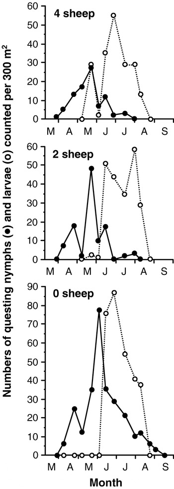
Fig. 11. The numbers of larvae (○) and nymphs ([bull ]) of Ixodes ricinus picked up by blanket-dragging in each of three enclosures on hill grazings in Wales, UK, with different densities of sheep, the only significant host. From Randolph & Steele, 1985.
Similar estimates of the period of persistence of questing ticks were derived from counts of R. appendiculatus feeding on cattle in South Africa. Because there was no element of experimental manipulation in this case, it was not possible to dissect mortality from host-attachment as the cause of disappearance. Asterisks on Fig. 4a indicate that at the end of the feeding seasons, there are sometimes months when larvae and adults were counted despite an absence of adults and nymphs, respectively, that could have produced them n months previously. These are interpreted as those ticks that persisted on the vegetation for up to two months beyond their recruitment until they eventually found a host. This must happen throughout the feeding season for each stage, but only becomes apparent at the end of each season. From the monthly rate of decline in the numbers of ticks counted after recruitment has ceased, the mean daily rate of disappearance was estimated as 0·043 for three farms, i.e. ticks persisted on the vegetation for an average of 23 days (range 15–34 days), with 7% remaining after two months. There was no discernible difference between tick stages; one interpretation is that, as mortality rates decrease with successive stages of this tick (see below), the questing success rate does in fact increase through the life cycle, as with I. ricinus, presumably because greater size, and thus resistance to environmental stress, permits prolonged exposure on the vegetation. Alternatively, but less likely, larvae may have a relatively high questing success rate because of a greater abundance of, and/or contact rate with, hosts for larval R. appendiculatus other than cattle (Macleod, 1970).
Thus we see that the rate of host-attachment is perhaps the most difficult of the essential demographic processes (Fig. 1) to measure empirically, requiring a great deal of host-specific data necessarily collected under natural conditions. Fortunately, however, this parameter is one of the easiest to incorporate into a population model. It is a simple probability which, even if not known accurately, can be assigned a realistic value and tweaked according to relative host availability.
Natural rates of tick mortality
Natural field experiments
The final demographic process in any life history is death. Seasonally variable daily death rates are fixed by the specific local abiotic and biotic conditions, and then operate for the duration of each stage in the life cycle. While we commonly estimate daily rates empirically from observations on percent survival, in reality the latter is determined by the former together with the time-span, according to the simple equation:

where m is the daily mortality rate and t is the period in days over which that mortality acts. If, for example, hosts are scarce and host attachment rates are low, the period of questing will be prolonged; daily mortality will not increase (although possibly increases non-linearly with the age of the tick), but will operate for longer, and so the percentage survival will be reduced. To be of most versatile use, the daily probability of death should be quantified at as fine a resolution (temporal, spatial and phenomenological) as possible. Well-defined rates can always be combined subsequently for any particular use, but can rarely be dissected from data if the original measurements are too coarse. Ideally, seasonally variable daily mortality rates operating on each stage in each state (questing, feeding, developing) should be measured. This usually requires specific experimental, but natural, conditions, and has rarely been achieved.
By excluding sheep from one of the enclosures described above (Randolph & Steele, 1985), estimates could be made of the daily mortality rates for larval (0·015) and nymphal (0·031) I. ricinus questing on a Welsh hillside between June and August or September, respectively (Fig. 11). Normally, however, in the presence of hosts the nymphs would not suffer such high mortality, because this estimate includes some element of death by starvation for nymphs active from April onwards. For larvae not active until mid-June, this specific cause of mortality was probably minimal before mid-August, and the above estimate may be realistic – it would permit c. 40% of the unfed larval population to survive the 2 month questing season here. Although highly specific in place and time, these estimates highlight the potential importance of biotic agents of mortality, such as predators, parasites or microbial infections, in habitats where saturation deficit, and therefore abiotic stress, is typically low throughout the summer.
Field observations within containers
So that survivors may be recovered and counted, most estimates of tick mortality have involved the use of containers within natural habitats (Branagan, 1973; Daniel et al. 1976; Gray, 1981; Daniels et al. 1996; Bertrand & Wilson, 1997). These exclude most predators, but are designed so that ticks are fully exposed to ambient conditions through plastic or nylon mesh walls. Ticks, however, actively select their resting positions within their architecturally diverse microhabitats, which may well offer higher moisture and more buffered temperature conditions than are found within containers. An accident during observations on larval R. appendiculatus in Kenya (Branagan, 1973) illustrates this point convincingly. Larvae from one batch escaped from their container and survived about four times as long as those which did not. It appears that they positioned themselves relative to the stomata on the grass stems so as to benefit from the raised transpirational humidities both before and after temporary closure of stomata during brief periods of evaporative stress. These larvae eventually succumbed only during periods of more prolonged arrested transpiration. Branagan (1973) concluded ‘The association between the climatic recordings and survival within containers cannot therefore be related to the survival of emerged instars which have access to transpirational microclimates – i.e. those under natural conditions.’
Nevertheless, container-derived estimates are the most common tools currently available for comparing relative mortality rates for ticks at various stages of their development or activity, in different habitats and at different seasons. Examples from studies in the Czech Republic (Daniel et al. 1976, 1977; and see chapter by Daniel et al. in this Supplement) and Ireland (Gray, 1981) (Table 1) illustrate some general principles. For comparability across different seasons, durations and stages, the observations on percentage survival (or mortality) of each exposed group of ticks have been translated into daily mortality rates, using the equation described above. Where available, the estimates for each stage were very similar from the two sets of studies, apart from the very much higher over-winter mortality of developing larvae and developing eggs in the Czech Republic than in Ireland, presumably related to the harshness of the continental winter. Engorged nymphs appeared to suffer least from this, but this stage was consistently more robust (as are nymphs of I. scapularis when exposed to the cold – Vandyk et al. 1996). Unfed larvae exposed in July suffered very high daily mortality (0·0067) until October, but much lower mortality (0·0018) over-winter, as would be expected from both the greater tick activity and the moisture stress typical of late summer. Despite the very high percentage hatch of eggs laid by females in Ireland, only c. 40% of larvae became active and reached the top of the activity tubes a few weeks later (Gray, 1981, 1982). Also, as expected, the mortality rates of ticks exposed in open meadows, and even on forest edges, were consistently very much higher than those in forests (Daniel et al. 1976, 1977).

Overall, the mortality rates estimated from these studies are much lower than the theoretical requirements for population regulation. A working model can be based on the expectation of decreasing natural mortality rates with successive, increasingly robust, life stages. This was indeed observed for R. appendiculatus, whose daily mortality rates were 0·019–0·070 for questing larvae, 0·017–0·029 for questing nymphs and 0·005–0·011 for questing adults confined in quasi-natural conditions in Zimbabwe and Zambia (calculated from survival data given in Short et al. 1989; Pegram & Banda, 1990), and is not contradicted by the above estimates for I. ricinus. We can therefore postulate that, on average, for a tick species with a mean fecundity of 2000 eggs, 5% survival from eggs to larvae, 10% survival from larvae to nymphs and 20% survival from nymphs to fully reproductive adults would theoretically allow the equilibrium state, i.e. one egg-laying female tick replacing herself per generation (Randolph, 1998). Although these are merely conveniently rounded numbers, they do allow some idea of the average inter-stadial mortality necessary to prevent exponential population increase in such fecund organisms. 20% survival requires a daily mortality rate of 0·0176 over a 3 month nymph-adult inter-stadial period, decreasing to 0·0044 if the inter-stadial period lasts 12 months. Likewise, 10% survival requires daily mortality rates of 0·0252–0·0063 for 3–12 month inter-stadial periods. These are approximately an order of magnitude greater than any observed for I. ricinus in container experiments (Table 1). Either mortality from abiotic causes within containers in temperate climates is much lower than occurs naturally, in contradiction to Branagan's (1973) observations in the tropics, or the vast majority of ticks die during processes prevented by containers, such as feeding or falling prey to predators.
It is clear that, with no realistic empirical estimates of absolute mortality rates, we lack a fundamental component for use in population models. Fortunately, the continuous production, more or less throughout the year, of new recruits into the tick populations of tropical and sub-tropical regions (Fig. 4) allows the calculation, not of absolute mortality rates, but of monthly relative indices of mortality. Standard census data on either questing or cattle-feeding R. appendiculatus of all stages in natural open-field situations at 11 sites in East and southern Africa yielded monthly inter-stadial mortality indices in the form of k values (Randolph, 1994a, 1997). These are estimated by subtracting the monthly log10(numbers+1) of one stage of ticks (e.g. nymphs) from the log10(numbers+1) of preceding stage (e.g. larvae) with the appropriate time interval equivalent to the development period (Varley, Gradwell & Hassell, 1973). By seeking correlations with these mortality indices, it was possible to identify the seasonally variable drivers of mortality, not only climate but also those biotic factors responsible for tick population regulation.
Natural population regulation in ticks
Ticks appear to be subjected to unusually intense mechanisms of natural population regulation. For organisms with such high birth rates, several thousand eggs per female, the potential for wide fluctuations in population size is large (Begon, Harper & Townsend, 1996). Yet regular sampling of various species over a number of years shows that ticks are typified by remarkably constant population sizes, varying annually by considerably less than one order of magnitude (see examples in Figs. 4 and 5, references in Randolph, 1994a, 1997). Population regulation about a fairly constant equilibrium level can be brought about only if the rates of one or more of the demographic processes vary with population density. Death rates must increase, or birth rates must decrease, with increasing density. Only biotic agents can respond to population density in this way, although not all such agents necessarily do so.
Analyses of R. appendiculatus populations have shown that inter-stadial mortality does indeed increase with increasing density of ticks of the stage preceding that inter-stadial phase (Fig. 12) (Randolph, 1994a, 1997). Furthermore, population regulation occurred at a level rarely seen in free-living populations of arthropods. Both the amount of density dependence (the regression coefficient, b, when the mortality index is regressed on tick density) and its predictability (R2 value for the same regression) are unusually high: of 22 observations of density-dependent mortality, 86% showed values of b between 0·51 and 2·0 (compared with 35% of observations on insects – Stubbs, 1977), while 73% gave R2 values [ges ]0·5. Such intensity is more likely to arise from an intimate biological interaction involving host immunity rather than the more diffuse ecological interaction of predation or parasitism, although the latter may possibly also contribute.

Fig. 12. Significant density-dependent relationships between the index of mortality from nymphs to adults and the log number of Rhipicephalus appendiculatus nymphs ([bull ]), and from larvae to nymphs and the log number of R. appendiculatus larvae (○), at Kirundo, Burundi (a) and (c) and Gulu, South Africa (b) and (d). Deviations from the regressions are significantly related to rainfall at Kirundo. Re-drawn from Randolph, 1994a, 1997.
Acquired resistance to feeding ticks can act in a density-dependent manner both in tick–cattle and tick–rodent interactions (Sutherst et al. 1979; Randolph, 1979, 1994b) and has been observed in many natural tick–host interactions (reviewed in Rechav, 1992; see chapter by Brossard & Wikel in this Supplement). Its effects may operate both intra- and inter-stadially (Jongejan et al. 1989; Walker, Fletcher & Todd, 1990), and vary with host type, such as breeds of cattle (Utech, Seifert & Wharton, 1978; Rechav, 1992; Moran, Nigarura & Pegram, 1996) and species of rodents. For example, woodmice (Apodemus spp.) do not, but voles (Clethrionomys glareolus) do acquire effective resistance against feeding larvae of Ixodes spp., resulting in reduced engorged weight and reduced survival to the nymphal stage (Randolph, 1979, 1994b; Dizij & Kurtenbach, 1995).
As expected on theoretical grounds, the observed strength of density dependence operating in R. appendiculatus populations was weaker nearer to the edge of the tick's geographical range, where less favourable abiotic conditions cause greater deviations from the density-dependent relationship, and for earlier developmental phases because the smaller immature stages are more vulnerable to these adverse abiotic factors (Fig. 12). The absence of an apparent density-dependent relationship for the adult-to-larval stage (with one exception) is merely an extension of this pattern; it is not that acquired resistance, elicited either by adults or larvae, does not affect the numbers of eggs produced or the success of feeding by larval ticks, as they have been shown to do (Chiera, Newson & Cunningham, 1985; Fivaz & Norval, 1990; Walker et al. 1990), but rather that even greater susceptibility of eggs and larvae to variable abiotic factors will swamp any biotic factors. These abiotic factors typically involved moisture availability to the eggs and larvae, measured in terms of rainfall or relative humidity, but probably more precisely dependent on soil moisture (Fig. 13) (see Guerra et al. 2002 for similar conclusions concerning I. scapularis in the mid-west of the USA). High mortality occurs where it is both too dry (typical of East Africa) and too wet (at the wettest site of South Africa), and also where development periods are prolonged in the coolest parts of South Africa (not shown). Sensitivity to moisture stress also introduces deviations from the density-dependent regressions for the larva–nymph and nymph-adult stages, as dry seasons impose exceptionally high mortality on all stages simultaneously (Fig. 12) (Randolph, 1994a).

Fig. 13. Significant relationships between the index of mortality from females to larvae of Rhipicephalus appendiculatus and moisture conditions during egg development, (a) rainfall at Kirundo, Burundi and (b) minimum % relative humidity at Gulu, South Africa. The bracketed outlier in (a) refers to the mortality during egg development in a month of low rainfall in the middle of the wet season, when soil moisture was likely to be high. Re-drawn from Randolph, 1994a, 1997.
Thus, even in the absence of precise estimates of absolute mortality rates, we may combine the theoretical limits based on known tick fecundity with a quantitative understanding of the abiotic and biotic determinants, sufficient to generate a working population model (Randolph & Rogers, 1997) (and see below).
ECOLOGICAL AND EPIDEMIOLOGICAL CONSEQUENCES OF TICK–HOST INTERACTIONS
Inter-specific patterns of tick–host relationships
Vertebrate hosts are absolutely necessary, of course, but not sufficient on their own for the presence of ticks. Animals upon which ticks can feed are more or less ubiquitous, and yet not all ticks are found on all apparently available hosts. Most tick species are less widely distributed than their principal hosts on both local and continental scales (Kitron et al. 1992; Cumming, 1999). Although different stage-specific requirements may account for some of this, Cumming (1999, 2002) concluded that climate, rather than vegetation or host distributions, limits the species ranges of most African ticks. Taking an explicitly evolutionary, global approach, it has been concluded that restrictions imposed by biogeography and ecological specificity, rather than by host specificity, lead to the observed host-association patterns (Klompen et al. 1996). This is not surprising, given the low specificity of most tick–host relationships. I. ricinus in Europe and I. scapularis in the USA feed on virtually any vertebrate of any class (mammals, birds or reptiles, but not amphibia) with which they come into contact (Milne, 1949; Anderson, 1991; Apperson et al. 1993). Other tick species show variable host specificity at each taxonomic level, some restricted merely to particular classes of vertebrates, others largely to particular orders within classes (e.g. the Carnivora, Artiodactyla, Rodentia among others), and a few apparently species-specific. Taking into account the many different sorts of biases introduced by collection practices and intensity (see also Klompen et al. 1996), Cumming (1998) showed convincingly that, although some may be classified as true specialists, the majority of the huge assemblage of African ticks are generalists to some degree. As contrasting examples of specialists, he cites Dermacentor circumguttatus, found on elephants but not on the many other sympatric mammals (i.e. host specificity), and Ixodes matopi, found only on granite kopjes where hyraxes and klipspringers are available as hosts (i.e. ecological specificity).
In general, therefore, ticks may be seen as opportunists, limited by abiotic constraints on where they can quest. Superimposed on this are the physical, behavioural and immunological characteristics of vertebrates which determine the differential distribution of ticks amongst their host species. This has significant consequences for the ecology of the tick, and for the transmission potential of any dependent pathogens.
Because vertebrate species are differentially competent to support the transmission of various tick–borne pathogens, the distribution of ticks amongst different host species will have an impact on the basic reproduction number, R0, of the pathogens. Non-competent hosts, for example, have been credited with having a zooprophylactic effect by decreasing the infection prevalence in the tick population (Spielman et al. 1985; Matuschka et al. 1992, 2000), but they may in fact have the opposite effect. Any host species that feeds enough ticks to reduce the overall infection prevalence in questing ticks of the next stage by diverting them away from transmission-competent host species, would be likely to increase the tick population density (and therefore the density of infected ticks – see above) by improving the chances of successful tick feeding. Deer seem to have played this role in relation to several tick-borne pathogens in northern temperate regions. In the USA and Denmark, the increase in incidence of Lyme borreliosis has been correlated with the increasing density and distribution of deer (Spielman et al. 1985; Jensen & Frandsen, 2000; Jensen et al. 2000). In parts of Europe, the risk of tick-borne encephalitis has been positively related to the presence of deer (Zeman & Januska, 1999; Hudson et al. 2001), not because deer can transmit the virus, but because deer support I. ricinus populations. Similarly, new epidemics of Kyasanur Fever Disease in India appear to have been precipitated by a marked increase in human population during the 1950s: cattle newly introduced into forests, although not hosts for the virus, supported increased populations of ticks which infected humans as they gathered firewood (Hoogstraal, 1981).
The degree of zooprophylaxis depends on the relative proportion of the vector population fed by different host species, which is highly variable geographically, and may also change with human impacts on habitat structure (Allan, Keesing & Ostfeld, 2003). High mammalian diversity has been predicted to have a negative effect on the infection prevalence of B. burgdorferi in nymphal I. scapularis (LoGiudice et al. 2003), but will only reduce the density of infected nymphs if the density of competent hosts species declines sufficiently with increasing host diversity. Where competent transmission hosts are more or less completely replaced, rather than augmented, by non-competent host species, enzootic cycles may be severely limited. This is thought to account for the much lower prevalence of B. burgdorferi sensu stricto in nymphal ticks in the southeast, compared with the northeast, of the USA (Piesman, 2002), where refractory lizards rather than rodents are the major hosts for immature I. scapularis (Apperson et al. 1993). Likewise, where pheasants are locally very abundant in southern England, they feed such a large proportion of the nymphal I. ricinus population that B. afzelii, which is not transmitted by birds, evidently cannot persist (Kurtenbach et al. 1998). In this case, the end point of R0<1 is reached, thereby eliminating infection altogether. This particular case is largely artificial, created by unnaturally high densities of pheasants released from game farms in the interests of shooting. Usually, hosts large enough to carry very high individual infestation levels of ticks exist at low population densities and so do not necessarily feed any greater fraction of the total tick population than do smaller, abundant hosts such as rodents (Talleklint & Jaenson, 1994; Craine, Randolph & Nuttall, 1995). The western fence lizard in northern California, however, is both non-competent to transmit B. burgdorferi sensu lato and so abundant as to feed almost all of the nymphal I. pacifucus in some areas, thereby significantly reducing the infection prevalence in adults compared with nymphs (Lane & Quistad, 1998).
Intra-specific patterns of tick–host relationships
Causes of aggregated distributions of ticks amongst their hosts
Higher infestation levels on larger hosts are common to many sorts of parasites, and this applies not only between, but also within, host species (Milne, 1949; Matuschka et al. 1992; Craine et al. 1995; Moore & Wilson, 2002). Size is just one of a nexus of host characteristics that cause aggregated rather than random distributions of parasites amongst their hosts, seen habitually in macro-parasites (reviewed by Shaw, Grenfell & Dobson, 1998). As mentioned above, these may be physical, behavioural or immunological, which frequently, but not invariably, operate synergistically. Thus within many wild populations, sexually mature male hosts tend to be larger, often range more widely in search of mates, and may be immunologically compromised by their hormones (Peters, 2000). All these features would promote higher tick infestation levels on this fraction of the host population, as has indeed been observed (Randolph, 1975; Matuschka et al. 1992).
Underpinning these particular host features are variable levels of testosterone, and this hormone has been shown experimentally to have a direct impact on resistance to tick infestations (Hughes & Randolph, 2001a). Testosterone levels were manipulated in voles, C. glareolus, and wood-mice, A. sylvaticus, within the normal physiological range seen in the wild. When exposed to repeated larval I. ricinus infestations, hosts with high hormone levels showed reduced innate and acquired resistance to tick feeding (Hughes & Randolph, 2001a). The innate resistance was manifested by the greater success with which larvae attached to high testosterone hosts independent of previous tick exposure. Successive infestations on voles were accompanied by a decrease in tick feeding success and survival, and this was significantly more marked in ticks fed on control voles than in those fed on voles implanted with testosterone (Fig. 14). Mice, which do not acquire resistance to I. ricinus, showed no such effects. Moreover, when reduced feeding success had been induced, by vaccination with tick salivary gland extract or four successive infestations, implantation with testosterone partially reversed that acquired resistance.
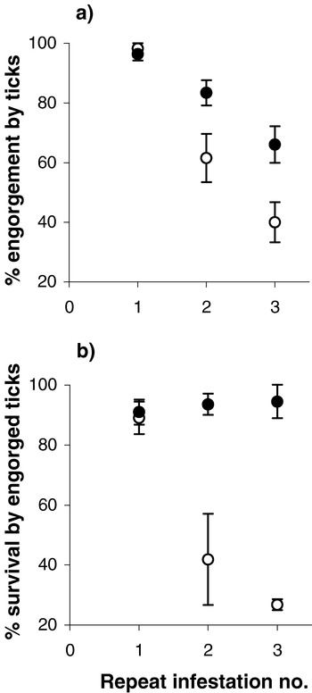
Fig. 14. Changes in mean (a) percent engorgement and (b) percent survival of Ixodes ricinus larvae with successive infestations on castrated voles (Clethrionomys glareolus) implanted with oil (○) or with testosterone ([bull ]). Data from Hughes & Randolph, 2001a.
These effects of testosterone will exacerbate the normal tendencies of acquired resistance to generate over-dispersed distributions of parasites (Anderson & Gordon, 1982; Pacala & Dobson, 1988), especially as those hosts with low resistance are also prone to high contact with ticks. High testosterone levels are also associated with increased locomotory activity in rodents (Randolph, 1977; Rowsewitt, 1986). Therefore, the same individual hosts are likely both to pick up most ticks and to feed them successfully. The ubiquitous presence of high testosterone levels in one fraction of wild populations, at least during part of each year, could offer a common basis for the typical over-dispersed distribution of diverse parasites amongst their hosts, and even amongst males themselves (Shaw et al. 1998).
In the case of pheasants as hosts, a field experiment showed that high infestation levels of ticks may themselves exacerbate further exposure to ticks via a negative impact on territoriality in male birds (Hoodless et al. 2002). Many sorts of parasites have an impact on male secondary sexual characteristics and female choice (reviewed in Clayton & Moore, 1997). When tick burdens on cock pheasants were reduced during March–August using a slow-release acaricide, the degree of wattle inflation was significantly improved (Fig. 15). This is an indicator of territorial status and a correlate of harem acquisition, and, correspondingly, harems were acquired by 44% of treated birds compared with only 22% of controls. Males that acquired females ranged over small areas on field edges, while those with no females ranged more widely in woods and the adjoining fields, thereby increasing their exposure to ticks. If non-territorial male pheasants do indeed feed a greater proportion of the tick population (which could not actually be observed in this experiment), ipso facto they support more tick-borne parasite transmission, which suggests therefore that ticks themselves could have a positive effect on the transmission dynamics of tick-borne parasites.

Fig. 15. Frequency distributions of the numbers of treated and control male pheasants that acquired different numbers of females, depending on their median wattle score (from 3 observations of each male in April). Score 1=no inflation of wattle, pinnae (ear tufts) not visible; 2=some inflation of wattles, pinnae discernible; 3=wattles fully inflated, pinnae erect. Number of females: open bars, 0; diagonal hatch, 1; stippled, 2; cross hatch, 3; black, 4–7. From Hoodless et al. 2002.
Consequences of aggregated distributions of ticks amongst their hosts
The population consequences of aggregated distributions of parasites amongst their hosts have been well revisited since Crofton's seminal work (Crofton, 1971a,b). With host mortality rates that increase with parasite burdens, and density-dependent constraints (immunological and other) on parasite survival, over-dispersion of parasites will stabilize the dynamical behaviour of host–parasite interactions (Anderson & May, 1978).
In addition, because ticks are also vectors, their over-dispersion increases the transmission potential of the dependent pathogens (Hasibeder & Dye, 1988; Randolph, 1995; Randolph et al. 1999) by focusing transmission efficiently within one highly infected fraction of the host population (Woolhouse et al. 1997, 1998). Quantitatively, this is an essential element in the persistence of those tick-borne pathogens that have very low R0 values. Babesia microti, for example, is maintained in rodent populations despite low mean infestation levels of the vector, I. trianguliceps (and possibly I. ricinus – Gray, von Stedingk & Gurtelschmid, 2002), and the very narrow window of transmission (Randolph, 1995). In this system, testosterone has yet another effect, directly increasing the transmissibility of B. microti by causing prolonged and more intense infections (Hughes & Randolph, 2001b). This occurs in exactly the same fraction of the host population that carries most ticks through other, synergistic effects of testosterone.
Because tick-borne transmission of pathogens depends on at least two tick stages feeding on the same host, one to transmit and the other to acquire, we can predict that the transmission potential will be improved if both tick stages show coincident aggregated distributions. For pathogens such as TBE virus with short-lived, even non-systemic, infections, this coincidence must be more or less synchronous, whereas for longer-lived, systemic infections (e.g. B. burgdorferi sensu lato) it need not be so. Such a phenomenon would easily arise if the same causal factors of aggregated distributions apply to both tick stages, as would all intrinsic host factors. Analysis of tick infestations on over 2500 individual rodents trapped in western Slovakia over three years supported this prediction (Randolph et al. 1999). The distributions of larval and nymphal I. ricinus were highly aggregated and, rather than being independent, the distributions of each stage were coincident so that the same c. 20% of hosts fed about 75% of both larvae and nymphs (Fig. 16). As a result, twice the number of infectible larvae fed alongside each potentially infected nymph compared with the null hypothesis of independent distributions, and estimated R0 values were >1, as required for virus persistence.

Fig. 16. The coincident aggregated frequency distributions of Ixodes ricinus larvae and nymphs on rodents (Clethrionomys glareolus and Apodemus flavicollis) from April to July in the Borská nízina lowland, Slovakia. At each intensity of larval infestation (X-axis), the numbers of hosts coincidentally feeding zero (open bars), 1–2 (light stippled), 3–4 (dark stippled) or 5–23 (black) nymphs are shown. Mean number of larvae co-feeding with a nymph=20. From Randolph et al. 1999.
The significance of this aspect of tick ecology in determining vector performance in nature is illustrated by the sympatric tick species in western Slovakia. Because of the different life cycle characteristics of D. reticulatus, the pattern of co-feeding larvae and nymphs does not apply to nearly the same extent as to I. ricinus. Development times of D. reticulatus are short, allowing the life cycle (apart from the egg stage) to be completed within a single year, with most larvae feeding one month before the nymphs. Thus, whereas only 3% of I. ricinus nymphs were recorded on hosts that were not carrying at least one larva, as many as 28% of D. reticulatus nymphs were not co-feeding with larvae of the same species (Randolph et al. 1999). Alternatively, as both species are competent vectors of TBE virus in the laboratory (Korenberg & Kovalevskii, 1994), the virus could potentially be exchanged between ticks of each species where they co-exist. These tick species, however, make differential use of voles and mice as hosts: more D. reticulatus were recorded on C. glareolus than on A. flavicollis, while I. ricinus showed the reverse host association (Randolph et al. 1999), so they do not co-feed to a significant extent. The principal host of I. ricinus, mice, are also the more efficient amplifiers of TBE virus (Labuda et al. 1993b, 1997). Factors such as these may explain why, amongst 18 species competent to transmit TBE virus in the laboratory (Korenberg & Kovalevskii, 1994), I. ricinus in Europe and I. persulcatus in Eurasia appear to be the only vectors and reservoirs responsible for long-term TBE virus survival in nature (Nuttall & Labuda, 1994). This is ecological specificity, leading to quantitative vectorial non-competence.
Of course, intra-specifically larvae are more likely to co-feed with other larvae than with nymphs, so could acquire the TBE virus from any trans-ovarially infected larva (Danielová et al. 2002). This, however, can only be an accessory route, insufficient on its own for two reasons. First, any resulting infected engorged larvae can only pass the infection on as they feed as infected nymphs on rodents, so we are back to nymphal-larval co-feeding transmission. Secondly, an essential quantitative element in transmission is amplification to offset the considerable natural mortality of ticks. If an infected nymph arising from a trans-ovarially infected larva, as above, feeds instead on a non-competent host but retains the virus and passes it trans-stadially to the adult stage, there would only be enormous diminution of infection prevalence in the tick population. Each larva, whether infected or not, on average gives rise to 0·01 adult female ticks (see above). Unless this were completely offset by trans-ovarial amplification, which is unlikely on the present evidence of 20% maternal transmission, 0·23–0·75% filial infection and the relatively low numbers of larvae that typically feed close together on any rodent (Danielová & Holubová, 1991; Danielová et al. 2002), TBE virus could not persist by this route. In fact, of 419 larval I. ricinus taken from 103 small mammals trapped in May and October within a TBE focus in the south of the Czech Republic, only 3 (1 unfed and 2 fed) were infected with TBE virus (Danielová et al. 2002).
PREDICTIVE MAPPING OF THE RISK FACTORS OF TICKS AS VECTORS
Distribution, abundance, seasonal dynamics and host relationships
For certain tick-borne pathogens, the transmission pathways are so robust that more or less wherever populations of competent ticks exist the pathogen will circulate to a greater or lesser extent. This appears to be true, for example, of B. burgdorferi sensu lato in Eurasia. In this case mapping the risk of infection in humans effectively becomes an exercise in mapping the distribution and abundance of the vector ticks. The use of statistical, pattern-matching approaches for predicting tick distributions has become increasingly sophisticated over the past two decades (Daniel & Kolar, 1990; Hugh-Jones et al. 1992; Daniel et al. 1998; Cumming, 1996, 2002; Estrada-Peña, 1998, 1999; Guerra et al. 2002). For further information on the application of Geographical Information Systems (GIS) for predicting tick and tick-borne diseases, the reader is directed to the accompanying chapter in this Supplement by Daniel, Kolar & Zeman. Briefly, within GIS statistical methods, such as discriminant analysis, logistic regression or co-kriging, can establish correlations between the presence of each tick species and selected environmental factors, either measured directly on the ground or remotely sensed from satellites (reviewed in Randolph, 2000). These correlations may then be used to predict relative habitat suitability across wide areas, beyond the original observations of tick presence or absence, thereby generating maps of the relative probabilities of tick presence. A higher probability may reflect greater abundance, although this has not been tested. The remotely sensed Normalized Difference Vegetation Index (NDVI), a measure of plant photosynthetic activity, has proved to be a key predictor of tick presence in all these studies. This index reflects moisture availability on the ground which, as we have seen above, is a major determinant of tick population performance and is indeed correlated with tick mortality rates (Randolph, 1994a).
For many tick-borne disease systems, however, the mere presence of the tick, even at high population densities, is not sufficient for a significant risk of infection. For the reasons outlined above, certain patterns of host relationships and tick seasonal dynamics may be required for robust enzootic cycles. In principle it should be possible to establish correlations between environmental conditions and tick–host relationships, because both vertebrate populations and tick questing habits are influenced by abiotic factors, but this has not yet been done on a wide scale. On the other hand, climatic correlates of particular patterns of tick seasonal dynamics have been identified and shown to be central to the accurate risk mapping of tick-borne encephalitis (Randolph, 2000; Randolph et al. 2000). At present, the association between a relatively rapid autumnal cooling in satellite-derived Land Surface Temperatures and both the continental distribution of TBE foci and the seasonal synchrony of larval and nymphal I. ricinus, is purely statistical. To move from this statistical prediction to a process-based biological explanation for the precise way in which this seasonal temperature profile generates larval-nymphal synchrony would give us a much more versatile tool. This is obviously the role of a fully functional tick population model and the raison d'être of this chapter.
Although not yet fully achieved for the complex system of I. ricinus in temperate regions, largely because of unresolved questions about diapause, a model for the more tractable system of R. appendiculatus in Africa has given encouraging results (Randolph & Rogers, 1997). Its predictions match the observed geographically variable patterns of seasonal dynamics closely (Fig. 17). This model is driven by just two climatic factors, temperature and rainfall. Therefore appropriate climatic data for any locality, accessible from an interpolated climate database (Hutchinson et al. 1995) or from meteorological satellite imagery, can be inserted into the model to predict the distributional limits, abundance and seasonal dynamics of the tick. Thus it should be possible to define the major risk factors for tick-borne diseases biologically in terms of population process rates, rather than relying on very much cruder statistical methods.

Fig. 17. Seasonal variation in the mean number of Rhipicephalus appendiculatus per host observed (○) and predicted by the population model ([bull ]); observed larvae×100, observed nymphs×10. (a) Gulu, South Africa, observations from Rechav, 1981; (b) Baker's Fort, northern Uganda, observations from Kaiser et al. 1991; (c) Ukunda, coastal Kenya, observations from Newson, 1978 did not include larvae. From Randolph & Rogers, 1997.
When this approach was applied to East Africa, the predicted spatial variation in relative numbers of adult ticks in Kenya, Uganda, Rwanda and Burundi showed vanishingly low R. appendiculatus abundance coinciding with the north-eastern edge of the recorded distribution (Fig. 18a). In Tanzania, however, although the model correctly predicted the observed declining abundance of ticks with increasing distance south- and east-wards from Lake Victoria (Tatchell & Easton, 1986), in central Tanzania the model fit was less good. It did not capture the recorded tick distribution as accurately as did the earlier statistical attempts (Rogers & Randolph, 1993; J. F. Toomer, unpublished observations) (Fig. 18b). Clearly there are still gaps in our knowledge that must be filled before this highly demanding biological approach can generate consistently reliable predictions over large geographical areas.

Fig. 18. Predictive maps of Rhipicephalus appendiculatus in East Africa compared with recorded presence ([bull ]) as compiled by Cumming (1996). (a) Relative abundance predicted by the population model (Randolph & Rogers, 1997) driven by temperature and rainfall taken from an interpolated climate database (Hutchinson et al. 1995). (b) Probabilities of tick presence driven by Advanced Very High Resolution Radiometer (AVHRR) satellite imagery (J. F. Toomer, 1996, unpublished observations).
CONCLUSIONS
Counting ticks, of all stages, in the field is the essential starting point of understanding tick ecology and tick-borne disease epidemiology. All such data are grist to the mill of analysis. Models, sometimes unhelpfully dismissed as ‘armchair ecology’, are the equally essential framework for that analysis, defining and refining our questions as we plug some gaps in our knowledge, but uncover yet more. If model predictions sometimes appear to run ahead of the known facts, that is the very purpose of models. They direct the collection of good quality data on vectors and vector-borne pathogens to match the increasingly sophisticated tools of analysis. The long, slow life cycle of ticks poses an extra challenge to tick ecologists working against the current insistence on short-term scientific productivity. The reward, a missing piece slotted neatly into the intricate jigsaw of the natural history of such important creatures, is worth the wait.
ACKNOWLEDGEMENTS
I am grateful to all my colleagues in many parts of the world who have contributed to my understanding of tick ecology. All past and present members of the Oxford Tick Research Group, particularly Chris Beattie, Noel Craine, Graeme Cumming, Rob Green, Andrew Hoodless, Vicki Hughes, Klaus Kurtenbach, Nick Ogden, Pat Nuttall and Mick Peacey, have helped to reveal the patterns and processes described here. David Rogers has been inspirational and operational in much of this work. I am grateful for financial support from The Royal Society, The Wellcome Trust and the Natural Environment Research Council of the UK.
References
REFERENCES
ALEKSEEV, A. N., DUBININA, H. V., RIJPKEMA, S. G. T. &
SCHOULS, L. M. (
1999).
Sexual transmission of Borrelia garinii by male Ixodes persulcatus ticks (Acari, Ixodidae).
Experimental and Applied Acarology
23, 165–169.CrossRefGoogle Scholar
ALLAN, B. F., KEESING, F. &
OSTFELD, R. S. (
2003).
Effect of forest fragmentation on Lyme disease risk.
Conservation Biology
17, 267–272.CrossRefGoogle Scholar
ANDERSON, J. F. (
1991).
Epizootiology of Lyme borreliosis.
Scandinavian Journal of Infectious Diseases Supplement
77, 23–34.Google Scholar
ANDERSON, R. M. &
GORDON, D. M. (
1982).
Processes influencing the distribution of parasite numbers within host populations with special emphasis on parasite-induced host mortalities.
Parasitology
85, 373–398.CrossRefGoogle Scholar
ANDERSON, R. M. &
MAY, R. M. (
1978).
Regulation and stability of host–parasite population interactions. I. Regulatory processes.
Journal of Animal Ecology
47, 219–249.Google Scholar
APPERSON, C. S., LEVINE, J. F., EVANS, T. L., BRASWELL, A. &
HELLER, J. (
1993).
Relative utilization of reptiles and rodents as hosts by immature Ixodes scapularis (Acari: Ixodidae) in the coastal plain of North Carolina, USA.
Experimental and Applied Acarology
17, 719–731.Google Scholar
BEGON, M., HARPER, J. L. &
TOWNSEND, C. R. (
1996).
Ecology (3rd edn.).
Oxford, Blackwell Scientific Publications.
BELOZEROV, V. N. (
1967).
[Larval diapause in the tick Ixodes ricinus L and its dependence on external conditions. IV. Interactions between exogenous and endogenous factors in the regulation of the larval diapause.] (In Russian).
Entomological Review
46, 447–451.Google Scholar
BELOZEROV, V. N. (
1970).
[Nymphal diapause in the tick Ixodes ricinus L. (Ixodidae). III. Photoperiodic reaction in unfed nymphs.] (In Russian.)
Parazitologiya
4, 139–145.Google Scholar
BELOZEROV, V. N. (
1982).
Diapause and biological rhythms in ticks. In
Physiology of Ticks (
ed. Obenchain, F. D. & Galun, R.), pp.
469–500.
Oxford, Pergamon Press.CrossRef
BELOZEROV, V. N. (
1998 a).
Role of two-step photoperiodic reaction in the control of development and diapause in the nymphs of Ixodes persulcatus.
Russian Journal of Zoology
2, 414–418.Google Scholar
BELOZEROV, V. N. (
1998 b).
Dynamics of gas exchange during development of Ixodid ticks: III. Dynamics of gas exchange in nymphs of the Ixodid ticks Hyalomma anatolicum Koch (Acari, Ixodidae) during active development and developmental diapause.
Entomological Review
78, 197–205.Google Scholar
BELOZEROV, V. N. &
NAUMOV, R. L. (
2001).
Photoperiodic control of nymphal diapause in the North American tick, Ixodes (Ixodes) scapularis Say (Acari: Ixodidae). In
IVth European Workshop of Invertebrate Ecophysiology (
ed. Kipyatkov, V. E.), p.
69.
St Petersburg, Russia.
BERKVENS, D. L., PEGRAM, R. G. &
BRANDT, J. R. A. (
1995).
A study of the diapausing behaviour of Rhipicephalus appendiculatus and R. zambesiensis under quasi-natural conditions in Zambia.
Medical and Veterinary Entomology
9, 307–315.Google Scholar
BERTRAND, M. R. &
WILSON, M. L. (
1997).
Microhabitat-independent regional differences in survival of unfed Ixodes scapularis nymphs (Acari: Ixodidae) in Connecticut.
Journal of Medical Entomology
34, 167–172.CrossRefGoogle Scholar
BRANAGAN, D. (
1973).
Observations on the development and survival of the Ixodid tick Rhipicephalus appendiculatus Neumann, 1901 under quasi-natural conditions in Kenya.
Tropical Animal Health and Production
5, 153–165.CrossRefGoogle Scholar
CAMPBELL, J. A. (
1948).
The life history and development of the sheep tick Ixodes ricinus Linaeus in Scotland, under natural and controlled conditions. PhD thesis, University of Edinburgh.
CERNY, M., DANIEL, M. &
ROSICKY, B. (
1974).
Some features of the developmental cycle of the tick Ixodes ricinus (L.) (Acarina: Ixodidae).
Folia Parasitologica
21, 85–87.Google Scholar
CHIERA, J. W., NEWSON, R. M. &
CUNNINGHAM, M. P. (
1985).
Cumulative effects of host resistance on Rhipicephalus appendiculatus Neumann (Acarina: Ixodidae) in the laboratory.
Parasitology
90, 401–408.CrossRefGoogle Scholar
CHMELA, J. (
1969).
On the developmental cycle of the common tick (Ixodes ricinus L.) in the north-Moravian natural focus of tick-borne encephalitis.
Folia Parasitologica
16, 313–319.Google Scholar
CLARK, D. D. (
1995).
Lower temperature limits for activity of several ixodid ticks (Acari: Ixodidae): effects of body size and rate of temperature change.
Journal of Medical Entomology
32, 449–452.CrossRefGoogle Scholar
clayton, d. h. &
moore, j. (ed.) (
1997).
Host–Parasite Evolution.
Oxford, Oxford University Press.
CRAINE, N. G., RANDOLPH, S. E. &
NUTTALL, P. A. (
1995).
Seasonal variation in the role of grey squirrels as hosts of Ixodes ricinus, the tick vector of the Lyme disease spirochaete, in a British woodland.
Folia Parasitologica
42, 73–80.Google Scholar
CROFTON, H. D. (
1971 a).
A quantitative approach to parasitism.
Parasitology
62, 179–193.Google Scholar
CROFTON, H. D. (
1971 b).
A model of host–parasite relationships.
Parasitology
63, 343–364.Google Scholar
CUMMING, G. S. (
1996).
The evolutionary ecology of African ticks. DPhil thesis, University of Oxford.
CUMMING, G. S. (
1998).
Host preference in African ticks (Acari: Ixodidae): a quantitative data set.
Bulletin of Entomological Research
88, 379–406.CrossRefGoogle Scholar
CUMMING, G. S. (
1999).
Host distributions do not limit the species ranges of most African ticks (Acari: Ixodida).
Bulletin of Entomological Research
89, 303–327.CrossRefGoogle Scholar
CUMMING, G. S. (
2002).
Comparing climate and vegetation as limiting factors for species ranges of African ticks.
Ecology
83, 255–268.CrossRefGoogle Scholar
DANIEL, M., CERNY, V., DUSBABEK, F., HONZAKOVA, E. &
OLEJNICEK, J. (
1976).
Influence of microclimate on the life cycle of the common tick Ixodes ricinus (L.) in thermophilic oak forest.
Folia Parasitologica
23, 327–342.Google Scholar
DANIEL, M., CERNY, V., DUSBABEK, F., HONZAKOVA, E. &
OLEJNICEK, J. (
1977).
Influence of microclimate on the life cycle of the common tick Ixodes ricinus (L.) in an open area in comparison with forest habitats.
Folia Parasitologica
24, 149–160.Google Scholar
DANIEL, M. &
KOLAR, J. (
1990).
Using satellite data to forecast the occurrence of the common tick Ixodes ricinus (L.).
Journal of Hygiene, Epidemiology, Microbiology and Immunology
45, 243–252.Google Scholar
DANIEL, M., KOLAR, J., ZEMAN, P., PAVELKA, K. &
SADLO, J. (
1998).
Predictive map of Ixodes ricinus high-incidence habitats and a tick-borne encephalitis risk assessment using satellite data.
Experimental and Applied Acarology
22, 417–433.CrossRefGoogle Scholar
DANIELOVÁ, V. (
2002).
Natural foci of tick-borne encephalitis and prerequisites for their existence.
International Journal of Medical Microbiology
291, S183–S186.CrossRefGoogle Scholar
DANIELOVÁ, V. &
HOLUBOVÁ, J. (
1991).
Transovarial transmission rate of tick-borne encephalitis virus in Ixodes ricinus ticks. In
Modern Acarology (
ed. Dusbabek, F. & Bukva, V.), pp.
7–10.
The Hague, Academia, Prague and SPB Academic Publishing.
DANIELOVÁ, V., HOLUBOVA, J., PEJCOCH, M. &
DANIEL, M. (
2002).
Potential significance of transovarial transmission in the circulation of tick-borne encephalitis virus.
Folia Parasitologica
49, 323–325.CrossRefGoogle Scholar
DANIELS, T. J., FALCO, R. C., CURRAN, K. L. &
FISH, D. (
1996).
Timing of Ixodes scapularis (Acari: Ixodidae) oviposition and larval activity in southern New York.
Journal of Medical Entomology
33, 140–147.CrossRefGoogle Scholar
DANIELS, T. J., FALCO, R. C. &
FISH, D. (
2000).
Estimating population size and drag sampling efficiency for the blacklegged tick (Acari: Ixodidae).
Journal of Medical Entomology
37, 357–363.CrossRefGoogle Scholar
DANIELS, T. J. &
FISH, D. (
1995).
Effect of deer exclusion on the abundance of immature Ixodes scapularis (Acari: Ixodidae) parasitizing small and medium-sized mammals.
Journal of Medical Entomology
32, 5–11.CrossRefGoogle Scholar
DISTER, S. W., FISH, D., BROS, S. M., FRANK, D. H. &
WOOD, B. L. (
1997).
Landscape characterization of peridomestic risk for Lyme disease using satellite imagery.
American Journal of Tropical Medicine and Hygiene
57, 687–692.CrossRefGoogle Scholar
DIZIJ, A. &
KURTENBACH, K. (
1995).
Clethrionomys glareolus, but not Apodemus flavicollis, acquires resistance to Ixodes ricinus L., the main European vector of Borrelia burgdorferi.
Parasite Immunology
17, 177–183.Google Scholar
EISEN, L., EISEN, R. J. &
LANE, R. S. (
2002).
Seasonal activity patterns of Ixodes pacificus nymphs in relation to climatic conditions.
Medical and Veterinary Entomology
16, 235–244.CrossRefGoogle Scholar
ESTRADA-PEÑA, A. (
1998).
Geostatistics and remote sensing as predictive tools of tick distribution: a cokriging system to estimate Ixodes scapularis (Acari: Ixodidae) habitat suitability in the United States and Canada from Advanced Very High Resolution Radiometer satellite imagery.
Journal of Medical Entomology
35, 989–995.CrossRefGoogle Scholar
ESTRADA-PEÑA, A. (
1999).
Geostatistics as predictive tools to estimate Ixodes ricinus (Acari: Ixodidae) habitat suitability in the western Paleartic from AVHRR satellite imagery.
Experimental and Applied Acarology
23, 337–349.CrossRefGoogle Scholar
FALCO, R. C., DANIELS, T. J. &
FISH, D. (
1995).
Increase in abundance of immature Ixodes scapularis (Acari: Ixodidae) in an emergent Lyme disease endemic area.
Journal of Medical Entomology
32, 522–526.CrossRefGoogle Scholar
FIELDEN, L. J. &
LIGHTON, J. R. B. (
1996).
Effects of water stress and relative humidity on ventilation in the tick Dermacentor andersoni (Acari: Ixodidae).
Physiological Zoology
69, 599–617.CrossRefGoogle Scholar
FILIPPOVA, N. A. (ed.) (
1985).
[Taiga Tick Ixodes persulcatus Schulze (Acarina, Ixodidae).] (In Russian).
Leningrad:
Nauka.
FIVAZ, B. H. &
NORVAL, R. A. I. (
1990).
Immunity of the ox to the brown ear tick Rhipicephalus appendiculatus.
Experimental and Applied Acarology
8, 51–63.CrossRefGoogle Scholar
FOURIE, L. J., BELOZEROV, V. N. &
NEEDHAM, G. R. (
2001).
Ixodes rubicundus nymphs are short-day diapause-induced ticks with thermolabile sensitivity and desiccation resistance.
Medical and Veterinary Entomology
15, 335–341.CrossRefGoogle Scholar
GAEDE, K. &
KNÜLLE, W. (
1997).
On the mechanism of water vapour sorption from unsaturated atmospheres by ticks.
Journal of Experimental Biology
200, 1491–1498.Google Scholar
GIGON, F. (
1985).
Biologie d'Ixodes ricinus L. sur le Plateau Suisse – une contribution a l'écologie de ce vecteur. MS thesis, Université de Neuchâtel, Switzerland.
GILOT, B., BONNEFILLE, M., DEGEILH, B., BEAUCOURNU, J.-C., PICHOT, J. &
GUIGUEN, C. (
1994).
La colonisation des massifs forestiers par Ixodes ricinus (Linne, 1758) en France: utilisation du chevreuil, Capreolus capreolus (L. 1758) comme marqueur biologique.
Parasite
1, 81–86.Google Scholar
GLASS, G. E., SCHWARZ, B. S., MORGAN III, J. M., JOHNSON, D. T., NOY, P. M. &
ISRAEL, E. (
1995).
Environmental risk factor for Lyme disease identified with geographic information systems.
American Journal of Public Health
85, 944–948.CrossRefGoogle Scholar
GRAY, J. S. (
1981).
The fecundity of Ixodes ricinus (L.) (Acarina: Ixodidae) and the mortality of its developmental stages under field conditions.
Bulletin of Entomological Research
71, 533–542.Google Scholar
GRAY, J. S. (
1982).
The development and questing activity of Ixodes ricinus (L.) (Acari: Ixodidae) under field conditions in Ireland.
Bulletin of Entomological Research
72, 263–270.Google Scholar
GRAY, J. S. (
1985).
Studies on the larval activity of the tick Ixodes ricinus L. in Co. Wicklow, Ireland.
Experimental and Applied Acarology
1, 307–316.CrossRefGoogle Scholar
GRAY, J. S., KAHL, O., JANETZKI, C. &
STEIN, J. (
1992).
Studies on the ecology of Lyme disease in a deer forest in County Galway, Ireland.
Journal of Medical Entomology
29, 915–920.CrossRefGoogle Scholar
GRAY, J. S., VON STEDINGK, L. V. &
GURTELSCHMID, M. E. A. (
2002).
Transmission studies of Babesia microti in Ixodes ricinus ticks and gerbils.
Journal of Clinical Microbiology
40, 1259–1263.CrossRefGoogle Scholar
GUERRA, M., WALKER, E., JONES, C. J., PASKEWITZ, S., CORTINAS, M. R., SANCIL, A., BECK, L., BOBO, M. &
KITRON, U. (
2002).
Predicting the risk of Lyme disease: habitat suitability for Ixodes scapularis in the north central United States.
Emerging Infectious Diseases
8, 289–297.CrossRefGoogle Scholar
HASIBEDER, G. &
DYE, C. M. (
1988).
Population dynamics of mosquito-borne disease: persistence in a completely heterogeneous environment.
Theoretical Population Biology
33, 31–53.CrossRefGoogle Scholar
HOODLESS, A. N., KURTENBACH, K., NUTTALL, P. A. &
RANDOLPH, S. E. (
2002).
The impact of ticks on pheasant territoriality.
Oikos
96, 245–250.CrossRefGoogle Scholar
HOOGSTRAAL, H. (
1981).
Changing patterns of tick-borne diseases in modern society.
Annual Review of Entomology
26, 75–99.CrossRefGoogle Scholar
HUDSON, P. J., RIZZOLI, A., ROSA, R., CHEMINI, C., JONES, L. D. &
GOULD, E. A. (
2001).
Tick-borne encephalitis virus in northern Italy: molecular analysis, relationships with density and seasonal dynamics of Ixodes ricinus.
Medical and Veterinary Entomology
15, 304–313.CrossRefGoogle Scholar
HUGH-JONES, M., BARRE, N., NELSON, G., WEHNES, K., WARNER, J., GARVIN, J. &
GARRIS, G. (
1992).
Landsat-TM identification of Amblyomma variegatun (Acari: Ixodidae) habitats in Guadeloupe.
Remote Sensing of the Environment
40, 43–55.CrossRefGoogle Scholar
HUGHES, V. L. &
RANDOLPH, S. E. (
2001 a).
Testosterone depresses innate and acquired resistance to ticks in natural rodent hosts: a force for aggregated distributions of parasites.
Journal of Parasitology
87, 49–54.Google Scholar
HUGHES, V. L. &
RANDOLPH, S. E. (
2001 b).
Testosterone increases the transmission potential of tick-borne parasites.
Parasitology
123, 365–371.Google Scholar
HUTCHINSON, M. F., NIX, H. A., McMAHON, J. P. &
ORD, K. D. (
1995).
Africa. A topographic and climate database. In
Centre for Resources and Environmental Studies, Canberra, The Australian National University.
JENSEN, P. M. &
FRANDSEN, F. (
2000).
Temporal risk assessment for Lyme borreliosis in Denmark.
Scandinavian Journal of Infectious Diseases
35, 539–544.Google Scholar
JENSEN, P. M., HANSEN, H. &
FRANDSEN, F. (
2000).
Spatial risk assessment for Lyme borreliosis in Denmark.
Scandinavian Journal of Infectious Diseases
35, 545–550.Google Scholar
JONGEJAN, F., PEGRAM, R. G., ZIVKOVIC, D., HENSEN, E. J., MWASE, E. T., THIELEMANS, M. J. C., COSSE, A., NIEWOLD, T. A., SAID, A. E. &
UILENBERG, G. (
1989).
Monitoring of naturally acquired and artificially induced immunity to Amblyomma variegatum and Rhipicephalus appendiculatus ticks under field and laboratory conditions.
Experimental and Applied Acarology
7, 181–189.CrossRefGoogle Scholar
KAISER, M. N., SUTHERST, R. W. &
BOURNE, A. S. (
1982).
Relationship between ticks and zebu cattle in southern Uganda.
Tropical Animal Health Production
14, 63–74.CrossRefGoogle Scholar
KAISER, M. N., SUTHERST, R. W. &
BOURNE, A. S. (
1991).
Tick (Acarina: Ixodidae) infestations on zebu cattle in northern Uganda.
Bulletin of Entomological Research
81, 257–262.CrossRefGoogle Scholar
KAISER, M. N., SUTHERST, R. W., BOURNE, A. S., GORISSEN, L. &
FLOYD, R. B. (
1988).
Population dynamics of ticks on Ankole cattle in five ecological zones in Burundi and strategies for their control.
Preventive Veterinary Medicine
6, 199–222.CrossRefGoogle Scholar
KEMP, D. H. (
1968).
Physiological studies on hard ticks Ixodidae. PhD thesis, University of Edinburgh.
KITRON, U., JONES, C. J., BOUSEMAN, J. K., NELSON, J. A. &
BAUMGARTNER, D. L. (
1992).
Spatial analysis of the distribution of Ixodes dammini (Acari: Ixodidae) on white-tailed deer in Ogle county, Illinois.
Journal of Medical Entomology
29, 259–266.CrossRefGoogle Scholar
KITRON, U. &
KAZMIERCZAK, J. J. (
1997).
Spatial analysis of the distribution of Lyme disease in Wisconsin.
American Journal of Epidemiology
145, 558–566.CrossRefGoogle Scholar
KLOMPEN, J. S. H., BLACK, W. C., KEIRANS, J. E. &
OLIVER, J. H. (
1996).
Evolution of ticks.
Annual Review of Entomology
41, 141–161.CrossRefGoogle Scholar
KNULLE, W. &
RUDOLPH, D. (
1982).
Humidity relationships and water balance of ticks. In
Physiology of Ticks (
ed. Obenchain, F. D. & Galun, R.), pp.
43–70.
Oxford, Pergamon Press.CrossRef
KORENBERG, E. I. (
2000).
Seasonal population dynamics of Ixodes ticks and tick-borne encephalitis virus.
Experimental and Applied Acarology
24, 665–681.CrossRefGoogle Scholar
KORENBERG, E. I. &
KOVALEVSKII, Y. V. (
1994).
A model for relationships among the tick-borne encephalitis virus, its main vectors, and hosts.
Advances in Disease Vector Research
10, 65–92.CrossRefGoogle Scholar
KURTENBACH, K., PEACEY, M. F., RIJPKEMA, S. G. T., HOODLESS, A. N., NUTTALL, P. A. &
RANDOLPH, S. E. (
1998).
Differential transmission of the genospecies of Borrelia burgdorferi sensu lato by game birds and small rodents in England.
Applied and Environmental Microbiology
64, 1169–1174.Google Scholar
LABUDA, M., AUSTYN, J. M., ZUFFOVA, E., KOZUCH, O., FUCHSBERGER, N., LYSY, J. &
NUTTALL, P. A. (
1996).
Importance of localized skin infection in tick-borne encephalitis virus transmission.
Virology
219, 357–366.CrossRefGoogle Scholar
LABUDA, M., JONES, L. D., WILLIAMS, T., DANIELOVA, V. &
NUTTALL, P. A. (
1993 a).
Efficient transmission of tick-borne encephalitis virus between cofeeding ticks.
Journal of Medical Entomology
30, 295–299.Google Scholar
LABUDA, M., KOZUCH, O., ZUFFOVA, E., ELECKOVA, E., HAILS, R. S. &
NUTTALL, P. A. (
1997).
Tick-borne encephalitis virus transmission between ticks cofeeding on specific immune natural rodent hosts.
Virology
235, 138–143.CrossRefGoogle Scholar
LABUDA, M., NUTTALL, P. A., KOZUCH, O., ELECKOVA, E., WILLIAMS, T., ZUFFOVA, E. &
SABO, A. (
1993 b).
Non-viraemic transmission of tick-borne encephalitis virus: a mechanism for arbovirus survival in nature.
Experientia
49, 802–805.Google Scholar
LANE, R. S. &
QUISTAD, G. B. (
1998).
Borreliacidal factor in the blood of the Western Fence Lizard (Sceloporus occidentalis).
Journal of Parasitology
84, 29–34.CrossRefGoogle Scholar
LEES, A. D. &
MILNE, A. (
1951).
The seasonal and diurnal activities of individual sheep ticks (Ixodes ricinus).
Parasitology
41, 180–209.CrossRefGoogle Scholar
LIGHTON, J. R. B. &
FIELDEN, L. J. (
1995).
Mass scaling of standard metabolism in ticks – a valid case of low metabolic rates in sit-and-wait strategists.
Physiological Zoology
68, 43–62.CrossRefGoogle Scholar
LOGIUDICE, K., OSTFELD, R. S., SCHMIDT, K. A. &
KEESING, F. (
2003).
The ecology of infectious disease: effects of host diversity and community composition on Lyme disease risk.
Proceedings of the National Academy of Sciences, USA
100, 567–571.CrossRefGoogle Scholar
LOYE, J. E. &
LANE, R. S. (
1988).
Questing behavior of Ixodes pacificus (Acari: Ixodidae) in relation to meteorological and seasonal factors.
Journal of Medical Entomology
25, 391–398.CrossRefGoogle Scholar
MACLEOD, J. (
1935).
Ixodes ricinus in relation to its physical environment. II. The factors governing survival and activity.
Parasitology
27, 123–144.Google Scholar
MACLEOD, J. (
1936).
Ixodes ricinus in relation to its physical environment. IV. An analysis of the ecological complexes controlling distribution and activities.
Parasitology
28, 295–319.CrossRefGoogle Scholar
MACLEOD, J. (
1970).
Tick infestation patterns in the Southern Province of Zambia.
Bulletin of Entomological Research
60, 253–274.CrossRefGoogle Scholar
MADDER, M., SPEYBROECK, N., BRANDT, J. &
BERKVENS, D. (
1999).
Diapause induction in adults of three Rhipicephalus appendiculatus stocks.
Experimental and Applied Acarology
23, 961–968.CrossRefGoogle Scholar
MATUSCHKA, F.-R., FISCHER, P., HEILER, M., RICHTER, D. &
SPIELMAN, A. (
1992).
Capacity of European animals as reservoir hosts for the Lyme disease spirochete.
Journal of Infectious Diseases
165, 479–483.CrossRefGoogle Scholar
MATUSCHKA, F.-R., SCHINKEL, T. W., KLUG, B., SPIELMAN, A. &
RICHTER, D. (
2000).
Relative importance of European rabbits for Lyme disease spirochaetes.
Parasitology
121, 297–302.CrossRefGoogle Scholar
MILNE, A. (
1949).
The ecology of the sheep tick, Ixodes ricinus L. Host relationships of the tick. Part 2. Observations on hill and moorland grazings in northern England.
Parasitology
39, 173–194.Google Scholar
MOORE, S. L. &
WILSON, K. (
2002).
Parasites as a viability cost of sexual selection in natural populations of mammals.
Science
297, 2015–2018.CrossRefGoogle Scholar
MORAN, M. C., NIGARURA, G. &
PEGRAM, R. G. (
1996).
An assessment of host resistance to ticks on cross-bred cattle in Burundi.
Medical and Veterinary Entomology
10, 12–18.CrossRefGoogle Scholar
NEEDHAM, G. R. &
TEEL, P. D. (
1991).
Off-host physiological ecology of ixodid ticks.
Annual Review of Entomology
36, 659–681.CrossRefGoogle Scholar
NEWSON, R. M. (
1978).
The life cycle of Rhipicephalus appendiculatus on the Kenyan coast. In
Tick-borne Diseases and their Vectors (
ed. Wilde, J. K. H.), pp.
46–50.
Edinburgh, CTVM, University of Edinburgh.
NICHOLSON, M. C. &
MATHER, T. N. (
1996).
Methods for evaluating Lyme disease risks using geographical information systems and geospatial analysis.
Journal of Medical Entomology
33, 711–720.CrossRefGoogle Scholar
NORVAL, R. A. I., LAWRENCE, J. A., YOUNG, A. S., PERRY, B. D., DOLAN, T. T. &
SCOTT, J. (
1991).
Theileria parva: influence of vector, parasite and host relationships on the epidemiology of theileriosis in southern Africa.
Parasitology
102, 347–356.CrossRefGoogle Scholar
NUTTALL, P. A. &
LABUDA, M. (
1994).
Tick-borne encephalitides. In
Ecological Dynamics of Tick-borne Zoonoses (
ed. Sonenshine, D. E. & Mather, T. N.), pp.
351–391.
New York, Oxford, Oxford University Press.
OCHANDA, H., YOUNG, A. S., WELLS, C., MEDLEY, G. F. &
PERRY, B. D. (
1996).
Comparison of the transmission of Theileria parva between different instars of Rhipicephalus appendiculatus.
Parasitology
113, 243–253.CrossRefGoogle Scholar
OGDEN, N. H., HAILS, R. S. &
NUTTALL, P. A. (
1998).
Interstadial variation in the attachment sites of Ixodes ricinus ticks on sheep.
Experimental and Applied Acarology
22, 227–232.CrossRefGoogle Scholar
OGDEN, N. H., RANDOLPH, S. E. &
NUTTALL, P. A. (
1997).
Natural Lyme disease cycle maintained via sheep by co-feeding ticks.
Parasitology
115, 591–599.CrossRefGoogle Scholar
PACALA, S. W. &
DOBSON, A. P. (
1988).
The relation between the number of parasites/host and host age: population dynamics causes and maximum likelihood estimation.
Parasitology
96, 197–210.CrossRefGoogle Scholar
PADGETT, K. A. &
LANE, R. S. (
2001).
Life cycle of Ixodes pacificus (Acari: Ixodidae): timing of development processes under field and laboratory conditions.
Journal of Medical Entomology
38, 684–693.CrossRefGoogle Scholar
PEGRAM, R. G. &
BANDA, D. S. (
1990).
Ecology and phenology of cattle ticks in Zambia: development and survival of free-living stages.
Experimental and Applied Acarology
8, 291–293.CrossRefGoogle Scholar
PERRET, J.-L., GUERIN, P. M., DIEHL, P.-A., VLIMANT, M. &
GERN, L. (
2003).
Darkness favours mobility and saturation deficit limits questing duration in Ixodes ricinus, the tick vector of Lyme disease in Europe.
Journal of Experimental Biology
206, 1809–1815.CrossRefGoogle Scholar
PERRET, J.-L., GUIGOZ, E., RAIS, O. &
GERN, L. (
2000).
Influence of saturation deficit and temperature on Ixodes ricinus tick questing activity in a Lyme borrelosis-endemic area (Switzerland).
Parasitology Research
86, 554–557.CrossRefGoogle Scholar
PETERS, A. (
2000).
Testosterone treatment is immunosuppressive in superb fairy-wrens, yet free-living males with high testosterone are more immunocompetent.
Proceedings of the Royal Society of London, B
267, 883–889.CrossRefGoogle Scholar
PIESMAN, J. (
2002).
Ecology of Borrelia burgdorferi sensu lato in North America. In
Lyme Borreliosis Biology, Epidemiology and Control (
ed. Gray, J. S., Kahl, O., Lane, R. S. & Stanek, G.), pp.
223–250.
Wallingford, CABI.CrossRef
RAND, P. W., LUBELCZYK, C., LAVIGNE, G. R., ELIAS, S., HOLMAN, M. S., LACOMBE, E. H. &
SMITH, R. P. J. (
2003).
Deer density and the abundance of Ixodes scapularis (Acari: Ixodidae).
Journal of Medical Entomology
40, 179–184.CrossRefGoogle Scholar
RANDOLPH, S. E. (
1975).
Patterns of distribution of the tick Ixodes trianguliceps Birula on its hosts.
Journal of Animal Ecology
44, 451–474.CrossRefGoogle Scholar
RANDOLPH, S. E. (
1977).
Changing spatial relationships in a population of Apodemus sylvaticus with the onset of breeding.
Journal of Animal Ecology
46, 653–676.CrossRefGoogle Scholar
RANDOLPH, S. E. (
1979).
Population regulation in ticks: the role of acquired resistance in natural and unnatural hosts.
Parasitology
79, 141–156.CrossRefGoogle Scholar
RANDOLPH, S. E. (
1993).
Climate, satellite imagery and the seasonal abundance of the tick Rhipicephalus appendiculatus in southern Africa: a new perspective.
Medical and Veterinary Entomologyy
7, 243–258.CrossRefGoogle Scholar
RANDOLPH, S. E. (
1994 a).
Population dynamics and density-dependent seasonal mortality indices of the tick Rhipicephalus appendiculatus in east and southern Africa.
Medical and Veterinary Entomology
8, 351–368.Google Scholar
RANDOLPH, S. E. (
1994 b).
Density-dependent acquired resistance to ticks in natural hosts, independent of concurrent infection with Babesia microti.
Parasitology
108, 413–419.Google Scholar
RANDOLPH, S. E. (
1995).
Quantifying parameters in the transmission of Babesia microti by the tick Ixodes trianguliceps amongst voles (Clethrionomys glareolus).
Parasitology
110, 287–295.CrossRefGoogle Scholar
RANDOLPH, S. E. (
1997).
Abiotic and biotic determinants of the seasonal dynamics of the tick Rhipicephalus appendiculatus in South Africa.
Medical and Veterinary Entomology
11, 25–37.CrossRefGoogle Scholar
RANDOLPH, S. E. (
1998).
Ticks are not insects: consequences of contrasting vector biology for transmission potential.
Parasitology Today
14, 186–192.CrossRefGoogle Scholar
RANDOLPH, S. E. (
2000).
Ticks and tick-borne disease systems in space and from space.
Advances in Parasitology
47, 217–243.CrossRefGoogle Scholar
RANDOLPH, S. E. (
2001).
The shifting landscape of tick-borne zoonoses: tick-borne encephalitis and Lyme borreliosis in Europe.
Philosophical Transactions of the Royal Society, B
356, 1045–1056.CrossRefGoogle Scholar
RANDOLPH, S. E. &
STEELE, G. M. (
1985).
An experimental evaluation of conventional control measures against the sheep tick Ixodes ricinus (L) (Acari: Ixodidae). II. The dynamics of the tick–host interaction.
Bulletin of Entomological Research
75, 501–518.Google Scholar
RANDOLPH, S. E., GREEN, R. M., PEACEY, M. F. &
ROGERS, D. J. (
2000).
Seasonal synchrony: the key to tick-borne encephalitis foci identified by satellite data.
Parasitology
121, 15–23.CrossRefGoogle Scholar
RANDOLPH, S. E., GREEN, R. M., HOODLESS, A. N. &
PEACEY, M. F. (
2002).
An empirical quantitative framework for the seasonal population dynamics of the tick Ixodes ricinus.
Internatioal Journal for Parasitology
32, 979–989.CrossRefGoogle Scholar
RANDOLPH, S. E., MIKLISOVÁ, D., LYSY, J., ROGERS, D. J. &
LABUDA, M. (
1999).
Incidence from coincidence: patterns of tick infestations on rodents facilitate transmission of tick-borne encephalitis virus.
Parasitology
118, 177–186.CrossRefGoogle Scholar
RANDOLPH, S. E. &
ROGERS, D. J. (
1997).
A generic population model for the African tick Rhipicephalus appendiculatus.
Parasitology
115, 265–279.CrossRefGoogle Scholar
RANDOLPH, S. E. &
STOREY, K. (
1999).
Impact of microclimate on immature tick-rodent interactions (Acari: Ixodidae): implications for parasite transmission.
Journal of Medical Entomology
36, 741–748.CrossRefGoogle Scholar
RECHAV, Y. (
1979).
Migration and dispersal patterns of three African ticks (Acari: Ixodidae) under field conditions.
Journal of Medical Entomology
16, 150–163.CrossRefGoogle Scholar
RECHAV, Y. (
1981).
Ecological factors affecting the seasonal activity of the brown ear tick Rhipicephalus appendiculatus. In
Tick Biology and Control (
ed. Whitehead, G. B. & Gibson, J. D.), pp.
187–191.
South Africa, Grahamstown University.
RECHAV, Y. (
1982).
Dynamics of tick populations (Acari: Ixodidae) in the Eastern Cape Province of South Africa.
Journal of Medical Entomology
19, 679–700.CrossRefGoogle Scholar
RECHAV, Y. (
1992).
Naturally acquired resistance to ticks – a global view.
Insect Science and its Application
13, 495–504.CrossRefGoogle Scholar
ROGERS, D. J. &
RANDOLPH, S. E. (
1993).
Distribution of tsetse and ticks in Africa: past, present and future.
Parasitology Today
9, 266–271.CrossRefGoogle Scholar
ROWSEWITT, C. N. (
1986).
Seasonal variation in activity rhythms of male voles: mediation by gonadal hormones.
Physiology and Behaviour
37, 797–803.CrossRefGoogle Scholar
SHAW, D. J., GRENFELL, B. T. &
DOBSON, A. P. (
1998).
Patterns of macroparasite aggregation in wildlife host populations.
Parasitology
117, 597–610.CrossRefGoogle Scholar
SHORT, N. J., FLOYD, R. B., NORVAL, R. A. I. &
SUTHERST, R. W. (
1989).
Survival and behaviour of unfed stages of the ticks Rhipicephalus appendiculatus, Boophilus decoloratus and B. microplus under field conditions in Zimbabwe.
Experimental and Applied Acarology
6, 215–236.Google Scholar
SHORT, N. J. &
NORVAL, R. A. I. (
1981).
The seasonal activity of Rhipicephalus appendiculatus Neumann 1901 (Acarina: Ixodidae) in the high veld of Zimbabwe Rhodesia.
Journal of Parasitology
67, 77–84.CrossRefGoogle Scholar
SONENSHINE, D. E. (
1991).
Biology of Ticks, vol. 1.
Oxford, Oxford University Press.
SPIELMAN, A., WILSON, M. L., LEVINE, J. F. &
PIESMAN, J. (
1985).
Ecology of Ixodes dammini-borne human babesiosis and Lyme disease.
Annual Review of Entomology
30, 439–460.CrossRefGoogle Scholar
STEELE, G. M. &
RANDOLPH, S. E. (
1985).
An experimental evaluation of conventional control measures against the sheep tick Ixodes ricinus (L) (Acari: Ixodidae). I. A unimodal seasonal activity pattern.
Bulletin of Entomological Research
75, 489–499.Google Scholar
STUBBS, M. (
1977).
Density dependence in the life-cycles of animals and its importance in K- and r-strategies.
Journal of Animal Ecology
46, 677–688.CrossRefGoogle Scholar
SUTHERST, R. W., UTECH, K. B. W., KERR, J. D. &
WHARTON, R. H. (
1979).
Density-dependent mortality of the tick Boophilus microplus, on cattle – further observations.
Journal of Applied Ecology
16, 397–403.CrossRefGoogle Scholar
TALLEKLINT, L. &
JAENSON, T. G. T. (
1994).
Transmission of Borrelia burgdorferi s.l. from mammal reservoirs to the primary vector of Lyme borreliosis, Ixodes ricinus (Acari: Ixodidae), in Sweden.
Journal of Medical Entomology
31, 880–886.Google Scholar
TALLEKLINT, L. &
JAENSON, T. G. T. (
1996).
Relationship between Ixodes ricinus density and prevalence of infection with Borrelia-like spirochetes and density of infected ticks.
Journal of Medical Entomology
33, 805–811.CrossRefGoogle Scholar
TALLEKLINT-EISEN, L. &
LANE, R. S. (
2000).
Efficiency of drag sampling for estimating population sizes of Ixodes pacificus (Acari: Ixodidae) nymphs in leaf litter.
Journal of Medical Entomology
37, 484–487.CrossRefGoogle Scholar
TATCHELL, R. J. &
EASTON, E. (
1986).
Tick (Acari: Ixodidae) ecological studies in Tanzania.
Bulletin of Entomological Research
76, 229–246.CrossRefGoogle Scholar
USPENSKY, I. (
1995).
Physiological age of Ixodid ticks: aspects of its determination and application.
Journal of Medical Entomology
32, 751–764.CrossRefGoogle Scholar
UTECH, K. B. W., SEIFERT, G. W. &
WHARTON, R. H. (
1978).
Breeding Australian Illawara shorthorn cattle for resistance to Boophilus microplus. I. Factors affecting resistance.
Australian Journal of Agricultural Research
29, 411–422.CrossRefGoogle Scholar
VAN ES, R. P., HILLERTON, J. E. &
GETTINBY, G. (
1998).
Lipid consumption in Ixodes ricinus (Acari: Ixodidae): temperature and potential longevity.
Bulletin of Entomological Research
88, 567–573.CrossRefGoogle Scholar
VANDYK, J. K., BARTHOLOMEW, D. M., ROWLEY, W. A. &
PLATT, K. B. (
1996).
Survival of Ixodes scapularis (Acari: Ixodidae) exposed to cold.
Journal of Medical Entomology
33, 6–10.CrossRefGoogle Scholar
VARLEY, G. C., GRADWELL, G. R. &
HASSELL, M. P. (
1973).
Insect Population Ecology: An Analytical Approach.
Oxford, Blackwell Scientific Publications.
WALKER, A. R. (
2001).
Age structure of a population of Ixodes ricinus (Acari: Ixodidae) in relation to its seasonal questing.
Bulletin of Entomological Research
91, 69–78.Google Scholar
WALKER, A. R., FLETCHER, J. D. &
TODD, L. (
1990).
Resistance between stages of the tick Rhipicephalus appendiculatus (Acari: Ixodidae).
Journal of Medical Entomology
27, 955–961.CrossRefGoogle Scholar
WILSON, M. L., ADLER, G. H. &
SPEILMAN, A. (
1985).
Correlation between abundance of deer and that of the deer tick, Ixodes dammini (Acari: Ixodidae).
Annals of the Entomological Society of America
78, 172–176.CrossRefGoogle Scholar
WOOLHOUSE, M. E. J., DYE, C., ETARD, J. F., SMITH, T., CHARLWOOD, J. D., GARNETT, G. P., HAGAN, P., HII, J. L. K., NDHLOVU, P. D., QUINNELL, R. J., WATTS, C. H., CHANDIWANA, S. K. &
ANDERSON, R. M. (
1997).
Heterogeneities in the transmission of infectious agents: implications for the design of control programs.
Proceedings of the National Academy of Sciences, USA
94, 338–342.CrossRefGoogle Scholar
WOOLHOUSE, M. E. J., ETARD, J.-F., DIETZ, K., NDHLOVU, P. D. &
CHANDIWANA, S. K. (
1998).
Heterogeneities in schistosome transmission dynamics and control.
Parasitology
117, 475–482.CrossRefGoogle Scholar
ZABICKA, J. (
1994).
[The tick-borne encephalitis in Poland.] (In Polish.)
Przegl Epidemiology
48, 197–203.Google Scholar
ZEMAN, P. &
JANUSKA, J. (
1999).
Epizootiologic background of dissimilar distribution of human cases of Lyme borreliosis and tick-borne encephalitis in a joint endenic area.
Comparative Immunology, Microbiology and Infectious Diseases
22, 247–260.CrossRefGoogle Scholar

Fig. 1. The structure of a population model for the tick Ixodes riciuns. Factors which determine the rates of the processes described within each box may be abiotic (solid arrow) or biotic (dotted arrow).

Fig. 2. The relationships between temperature and daily rates of inter-stadial development. Note the same pattern, but quantitative differences between stages (circles, larva–nymph; squares, nymph–adult; triangles, female–larva), and between species (filled symbols, Rhipicephalus appendiculatus; open symbols, Ixodes ricinus). Re-drawn from original data in Campbell, 1948; Branagan, 1973; Kaiser et al. 1988.

Fig. 3. Seasonal and geographical variation in daily rates of larva–nymph inter-stadial development rates predicted by day-degree summation models based on ambient temperatures. Squares, Ixodes ricinus in Dorset, UK ([squf ]) and Wales, UK (□); circles, Rhipicephalus appendiculatus in Kirundo, Burundi ([bull ]) and Gulu, South Africa (○). The grey symbols () show the effect of basing the predictions for Dorset on air, rather than soil, temperatures.

Fig. 4. Seasonal variation in the number of larval, nymphal and adult Rhipicephalus appendiculatus at (a) Gulu, South Africa (data from Rechav, 1982) and (b) Kirundo, Burundi (data from Kaiser et al. 1988). The grey arrows indicate which ticks of one life stage gave rise to which ticks of the next stage (according to Randolph, 1994a, 1997). In (a), ‘d’ marks the months of diapausing adults, and asterisks mark those adults and larvae which were counted after recruitment had apparently ceased (see text).

Fig. 5. Seasonal variation in the number of larval, nymphal and adult Ixodes ricinus in Dorset, UK. The arrows indicate which ticks of one life stage gave rise to which ticks of the next stage (according to Randolph et al. 2002). Asterisks mark show dates of first appearance of high-fat (newly recruited) nymphs and adults in the field.

Fig. 6. Seasonal changes in absolute frequency distributions of questing nymphal Ixodes ricinus with different fat content indices counted per 100 m2 in Dorset, UK, starting with late summer at the top in each of two years. Data for two monthly samples are presented in each histogram, showing the earlier data of each pair as filled bars and the later date hatched. In September/October when old and new recruits occur within the same sample, new recruits are shown by open bars. The vertical dotted line is purely to guide the eye.

Fig. 7. Seasonal variation in maximum air temperature (Ta) and numbers of questing larval (○) and nymphal ([bull ]) Ixodes ricinus at three sites in the UK (note that larval density is presented at 33% of observed level). Dotted and dashed lines indicate the temperature thresholds for the onset of seasonal activity of larvae and nymphs, respectively.

Fig. 8. Seasonal changes in the size (i.e. fat free weight) composition of populations of questing nymphal Ixodes ricinus during the life-span of a single cohort on Exmoor, UK 1998–1999. Sample dates and sizes are shown in the key. With permission from Randolph et al. 2002.

Fig. 9. Questing activity and attachment to rodents of Ixodes ricinus nymphs and larvae in relation to degrees of moisture stress in dry (left) and wet (right) experimental arenas. (a) maximum saturation deficit; (b) numbers of nymphs and (c) larvae counted per hour at 0900 and 2100 h (filled symbols) and 1200, 1500 and 1800 h (open symbols); (d) numbers of nymphs (circles) and larvae (diamonds) attached per rodent. Fresh ticks were added to the arenas on days 17 and 24 as indicated, and the dry arena was watered on day 24, both of which showed that quiescence rather than death was the cause of low questing activity. Data taken from Randolph & Storey, 1999.

Fig. 10. Theoretical changes in the numbers of questing ticks (Nt) through time (t) in the absence of hosts or the presence of hosts at different densities. Seasonal recruitment (which may be directly through development, or by reactivation of ticks after a period of behavioural diapause or quiescence) starts at time t0 and ceases at time t1. Re-drawn from Randolph & Steele, 1985.

Fig. 11. The numbers of larvae (○) and nymphs ([bull ]) of Ixodes ricinus picked up by blanket-dragging in each of three enclosures on hill grazings in Wales, UK, with different densities of sheep, the only significant host. From Randolph & Steele, 1985.

Table 1. Examples of mortality estimates for I. ricinus derived from observations on ticks within containers

Fig. 12. Significant density-dependent relationships between the index of mortality from nymphs to adults and the log number of Rhipicephalus appendiculatus nymphs ([bull ]), and from larvae to nymphs and the log number of R. appendiculatus larvae (○), at Kirundo, Burundi (a) and (c) and Gulu, South Africa (b) and (d). Deviations from the regressions are significantly related to rainfall at Kirundo. Re-drawn from Randolph, 1994a, 1997.

Fig. 13. Significant relationships between the index of mortality from females to larvae of Rhipicephalus appendiculatus and moisture conditions during egg development, (a) rainfall at Kirundo, Burundi and (b) minimum % relative humidity at Gulu, South Africa. The bracketed outlier in (a) refers to the mortality during egg development in a month of low rainfall in the middle of the wet season, when soil moisture was likely to be high. Re-drawn from Randolph, 1994a, 1997.

Fig. 14. Changes in mean (a) percent engorgement and (b) percent survival of Ixodes ricinus larvae with successive infestations on castrated voles (Clethrionomys glareolus) implanted with oil (○) or with testosterone ([bull ]). Data from Hughes & Randolph, 2001a.

Fig. 15. Frequency distributions of the numbers of treated and control male pheasants that acquired different numbers of females, depending on their median wattle score (from 3 observations of each male in April). Score 1=no inflation of wattle, pinnae (ear tufts) not visible; 2=some inflation of wattles, pinnae discernible; 3=wattles fully inflated, pinnae erect. Number of females: open bars, 0; diagonal hatch, 1; stippled, 2; cross hatch, 3; black, 4–7. From Hoodless et al. 2002.

Fig. 16. The coincident aggregated frequency distributions of Ixodes ricinus larvae and nymphs on rodents (Clethrionomys glareolus and Apodemus flavicollis) from April to July in the Borská nízina lowland, Slovakia. At each intensity of larval infestation (X-axis), the numbers of hosts coincidentally feeding zero (open bars), 1–2 (light stippled), 3–4 (dark stippled) or 5–23 (black) nymphs are shown. Mean number of larvae co-feeding with a nymph=20. From Randolph et al. 1999.

Fig. 17. Seasonal variation in the mean number of Rhipicephalus appendiculatus per host observed (○) and predicted by the population model ([bull ]); observed larvae×100, observed nymphs×10. (a) Gulu, South Africa, observations from Rechav, 1981; (b) Baker's Fort, northern Uganda, observations from Kaiser et al. 1991; (c) Ukunda, coastal Kenya, observations from Newson, 1978 did not include larvae. From Randolph & Rogers, 1997.

Fig. 18. Predictive maps of Rhipicephalus appendiculatus in East Africa compared with recorded presence ([bull ]) as compiled by Cumming (1996). (a) Relative abundance predicted by the population model (Randolph & Rogers, 1997) driven by temperature and rainfall taken from an interpolated climate database (Hutchinson et al. 1995). (b) Probabilities of tick presence driven by Advanced Very High Resolution Radiometer (AVHRR) satellite imagery (J. F. Toomer, 1996, unpublished observations).
 You have
Access
- 394
- Cited by