





1. Introduction
In Part 1 of this study, the influences of local and upstream pressure gradients (PGs) on high-Reynolds-number adverse-pressure-gradient (APG) turbulent boundary layers (TBLs) were examined, demonstrating that PG history can significantly modify the mean velocity profile. Building on those findings, the present paper focuses on the wall-normal structure of the mean streamwise velocity profile in APG TBLs and the development of a composite representation of this profile.
The mean velocity profile is of particular interest because it is directly associated with quantities of engineering relevance, such as the skin-friction drag generated by the TBL (Panton Reference Panton2005). More broadly, a well-resolved mean velocity profile is also a fundamental component in the development of mixing-length and eddy-viscosity models, which can be used to predict the Reynolds-stress distribution of the TBL (Subrahmanyam et al. Reference Subrahmanyam, Cantwell and Alonso2022). It also plays a central role in resolvent-based descriptions of wall-bounded turbulence, where the mean profile acts as the base flow that governs the amplification and organisation of coherent motions (Sharma & McKeon Reference Sharma and McKeon2013).
These utilities make accurate description of the mean velocity profile valuable for both simulations and experiments, particularly when quantities such as the Reynolds stresses or the wall-shear stress cannot be measured directly. The importance of such approaches also increases with the friction Reynolds number (
 $ \textit{Re}_{\tau }=\delta U_{\tau }/\nu$
), as numerical simulations become more expensive and experimental measurements of Reynolds stresses become increasingly difficult. Here,
 $\delta$
denotes the boundary-layer thickness (determined in this manuscript using the method of Lozier et al. Reference Lozier, Deshpande, Zarei, Lindić, Rowin and Marusic2025),
 $U_{\tau }$
is the friction velocity (related to the wall-shear stress through
 $\tau _w=\rho U_\tau ^2$
),
 $\rho$
is the density and
 $\nu$
is the kinematic viscosity. Throughout this study, the term high-
 $ \textit{Re}_{\tau }$
follows the arguments of Hutchins & Marusic (Reference Hutchins and Marusic2007), where an
 $ \textit{Re}_{\tau }\gtrsim 4000$
provides the scale separation indicative of high-Reynolds-number TBL behaviours.
For these reasons, the development of analytical expressions describing the mean velocity profile has been an enduring objective in wall-bounded turbulence research (Panton Reference Panton2005). Such descriptions take a variety of forms (e.g. the integral formulations of Cantwell et al. Reference Cantwell, Bilgin and Needels2022; Subrahmanyam et al. Reference Subrahmanyam, Cantwell and Alonso2022; Yang et al. Reference Yang, Chen, Zhang and Kunz2024; Shu & Xu Reference Shu and Xu2026); however, one widely used approach is the composite formulation. In composite models, the mean profile is constructed by combining expressions that represent the dominant physics of different regions of the boundary layer (e.g. the inner, overlap and wake regions) into a single continuous profile (see Nickels Reference Nickels2004). These formulations are typically expressed in terms of normalised variables, with the mean streamwise velocity
 $U$
and wall-normal coordinate
 $z$
scaled by the viscous velocity (
 $U_\tau$
) and length (
 $\nu /U_\tau$
) scales (denoted by the superscript ‘
 $+$
’).
It is well known that TBL statistics, including the mean velocity profile, depend on several flow parameters such as
 $ \textit{Re}_{\tau }$
, streamwise PGs and surface roughness. Consequently, developing a robust and generic composite representation of the mean velocity profile is challenging. Such a formulation must capture the underlying physics across the different regions of the boundary layer while remaining consistent with established high-fidelity datasets spanning a broad range of flow conditions.
1.1. Composite mean velocity profile formulations for the TBL
We briefly review the development of composite formulations for the mean velocity profile in TBLs. In the classical view, the composite profile follows a wall–wake structure consisting of two functional relationships commonly referred to as the ‘law of the wall’ and the ‘law of the wake’ (Coles Reference Coles1956; Marusic et al. Reference Marusic, McKeon, Monkewitz, Nagib, Smits and Sreenivasan2010)
 \begin{align} U^{+} =f(z^{+}) + {g}(\varPi ,\eta ), \end{align}
where the wall function,
 $f$
, depends on the viscous-scaled wall-normal distance (
 $z^{+}=zU_{\tau }/\nu$
), while the wake function,
 $\mathrm{g}$
, depends on the outer-scaled wall-normal distance (
 $\eta =z/\delta$
) and Coles’ wake-strength parameter,
 $\varPi$
.
The wall function can be further decomposed into two fundamental scaling laws obtained through a range of arguments (see Millikan Reference Millikan1938; Clauser Reference Clauser1956; Coles Reference Coles1956; Panton Reference Panton2005; Marusic et al. Reference Marusic, McKeon, Monkewitz, Nagib, Smits and Sreenivasan2010). The first applies very near the wall (
 $z^{+} \lesssim 5$
, i.e. in the viscous sublayer), where
 \begin{align} U^{+}=z^{+}, \end{align}
as required in the limit as
 $z^{+} \rightarrow 0$
. The second applies farther from the wall, while
 $\eta$
remains small
 \begin{align} U^{+} = \frac {1}{\kappa } \,\ln ( z^{+} ) + B, \end{align}
where
 $\kappa$
and
 $B$
are traditionally referred to as the von Kármán and additive constants (Marusic et al. Reference Marusic, Monty, Hultmark and Smits2013), respectively, although recent studies suggest that they should be regarded as coefficients that may depend on flow and boundary conditions (Monkewitz & Nagib Reference Monkewitz and Nagib2023). This classical logarithmic law is observed in the overlap region of canonical high-
 $ \textit{Re}_{\tau }$
TBLs and has been studied extensively (Marusic et al. Reference Marusic, McKeon, Monkewitz, Nagib, Smits and Sreenivasan2010).
Between the viscous sublayer and overlap region lies the buffer region, where neither scaling law applies exclusively. Its functional form is not well defined physically, and some studies (Long & Chen Reference Long and Chen1981; Afzal Reference Afzal1984) have further identified ‘mesolayers’ between the buffer and overlap regions. Accordingly, many studies have sought to combine the two classical scaling laws into a single expression for the near-wall mean velocity. For example, Van Driest (Reference Van Driest1956) derived a shear-stress relation that, when integrated, yields an integral expression for the streamwise velocity, although its practical use is not straightforward. Alternative expressions, such as those of Spalding (Reference Spalding1961) and Musker (Reference Musker1979), provide a single representation for the viscous sublayer and buffer regions (collectively termed the ‘inner’ region) and asymptotically recover the logarithmic law with increasing wall-normal distance.
Following these approaches, many composite formulations take the form
 \begin{align} U^{+} = U^{+}_{\textit{inner}}(z^{+})+U^{+}_{ov\textit{erlap}}(z^{+},\eta )+U^{+}_{w\textit{ake}}(\eta ,\varPi ), \end{align}
where separate analytical expressions describe the inner, overlap and wake regions of the TBL (see Chauhan et al. Reference Chauhan, Monkewitz and Nagib2009). If the boundary-layer thickness and friction velocity are known, these formulations contain only one free parameter,
 $\varPi$
, which may be obtained by fitting the composite profile to the measured mean velocity profile. Such formulations are therefore referred to here as one-parameter composite profiles. They typically provide good fits for ‘well-behaved’ canonical TBLs (i.e. smooth-wall, zero-pressure-gradient (ZPG) flows with minimal history effects; see Chauhan et al. Reference Chauhan, Monkewitz and Nagib2009), although some limitations remain.
For example, the boundary-layer thickness used in these formulations does not always correspond to a commonly, or easily, measured quantity (e.g.
 $\delta _{99}$
), and is sometimes treated as an additional fitting parameter. Further uncertainty arises in the wake region. The wake function,
 $\mathcal{W}$
, introduced by Coles (Reference Coles1956) was sinusoidal, such that the wake contribution was written as
 \begin{align} U^{+}_{w\textit{ake}}= \frac {2\varPi }{\kappa } \mathcal{W}(\eta ). \end{align}
Subsequent studies have instead used exponential functions (Nickels Reference Nickels2004; Chauhan et al. Reference Chauhan, Nagib and Monkewitz2007), polynomial functions (Jones et al. Reference Jones, Marusic and Perry2001) and other physically motivated models (for example, based on turbulent/non-turbulent interface interactions; Krug et al. Reference Krug, Philip and Marusic2017). Although these forms can produce good fits for particular TBLs, ambiguity regarding a generally applicable wake function persists. The classical wall–wake formulation of Coles (Reference Coles1956) and the one-parameter composite profile of Chauhan et al. (Reference Chauhan, Monkewitz and Nagib2009) are therefore primarily associated with canonical TBLs.
For PG TBLs specifically, the mean velocity profile depends not only on Reynolds number but also on both the local streamwise PG (Nagano et al. Reference Nagano, Tsuji and Houra1998; Monty et al. Reference Monty, Harun and Marusic2011; Harun et al. Reference Harun, Monty, Mathis and Marusic2013; Dróżdż et al. Reference Dróżdż, Elsner, Niegodajew, Vinuesa, Örlü and Schlatter2020 ; Deshpande et al. Reference Deshpande, Van Den Bogaard, Vinuesa, Lindić and Marusic2023) and the upstream PG history (Bobke et al. Reference Bobke, Vinuesa, Örlü and Schlatter2017; Vinuesa et al. Reference Vinuesa, Örlü, Sanmiguel Vila, Ianiro, Discetti and Schlatter2017; Pozuelo et al. Reference Pozuelo, Li, Schlatter and Vinuesa2022; Romero et al. Reference Romero, Zimmerman, Philip and Klewicki2023). However, there is currently no established mathematical framework for explicitly describing the mean velocity profile of generic PG TBLs. Although one-parameter composite profiles were not intended only for canonical flows, they generally do not describe non-canonical TBLs well, including certain regimes of streamwise PGs and/or surface roughness. For example, in PG flows without a wake region (e.g. sink flows), the overlap expression in (1.4) grows unboundedly, whereas physically the mean velocity should approach a constant value at the boundary-layer edge (i.e.
 $U^{+} \rightarrow U^{+}_\infty$
as
 $\eta \rightarrow 1$
). These limitations have motivated new composite formulations for specific non-canonical TBL classes, including generic PG TBLs (Nickels Reference Nickels2004), i.e. for both APG and favourable-pressure-gradient (FPG) conditions.
Accounting for streamwise PGs in a composite mean velocity formulation then requires at least one additional free parameter beyond
 $\varPi$
, yielding a two-parameter composite profile. Here, the local PG is quantified using Clauser’s PG parameter
 \begin{align} \beta = \frac {\delta ^\ast }{\tau _w}\left (\frac {{\rm d}P}{{\rm d}x}\right ) \!, \end{align}
where
 $\delta ^\ast$
denotes the displacement thickness and
 ${\rm d}P/{\rm d}x$
the streamwise gradient of the static pressure. The local PG strength may also be expressed using viscous scaling alone
 \begin{align} p_{x}^{+} = \frac {\nu }{\rho u_\tau ^3} \left ( \frac {{\rm d}P}{{\rm d}x} \right )\!. \end{align}
This viscous-scaled PG parameter,
 $p_{x}^{+}$
, is important because it arises naturally in composite formulations, specifically in the inner-region expression, through a Taylor-series expansion of the boundary-layer equations near the wall (Nickels Reference Nickels2004). The PG-related terms in this expansion are often neglected because
 $p_x^{+}$
is small in high-
 $ \textit{Re}_{\tau }$
TBLs (
 $p_{x}^{+}=\beta /\delta ^{*+}$
) and/or in flows with low-to-moderate PGs, but these terms do become significant in low-
 $ \textit{Re}_{\tau }$
PG TBLs and in flows subjected to strong PGs (Nickels Reference Nickels2004). However, we note that, for strong APGs, specifically as the flow approaches separation,
 $U_{\tau }$
is no longer considered a reliable scaling parameter. In this limit, Nickels (Reference Nickels2004) suggested the relevant scaling parameter is instead the pressure velocity,
 $U_p=\{(\nu /\rho )\, (\mathrm{d}P/\mathrm{d}x)\}^{1/3}$
, and it is unclear if the corresponding mean velocity profiles can be described within the original framework of Nickels (Reference Nickels2004), or the present formulation. As such, further work is needed to establish the appropriate scaling and formulation for APG TBLs in this limit.
Contributions of the inner, overlap and wake expressions from Nickels (Reference Nickels2004) as a function of (a)
 $p_x^{+}$
and (b)
 $z^{+}_{c}$
. The composite mean velocity profiles (solid lines) are the sum of the three individual expressions. A baseline dataset with
 $ \textit{Re}_{\tau }=5000$
was used to generate these profiles.

Figure 1. Long description
Panel A: A line graph shows the contributions of inner, overlap, and wake expressions to mean velocity profiles as a function of z+. The x-axis is labeled z+ and ranges from 10^1 to 10^4. The y-axis is labeled U+ and ranges from 0 to 35. Three solid lines represent different values of px+ (-0.02, 0, 0.02). Dashed lines indicate the contributions of inner, overlap, and wake expressions. Panel B: Another line graph shows the contributions of inner, overlap, and wake expressions to mean velocity profiles as a function of z+ for different values of zc+ (14.0, 12.0, 10.4). The x-axis is labeled z+ and ranges from 10^1 to 10^4. The y-axis is labeled U+ and ranges from 0 to 35. Three solid lines represent different values of zc+.
Accordingly, Nickels (Reference Nickels2004) reintroduced the
 $p_x^{+}$
-dependent terms and introduced a new parameter,
 $z^{+}_{c}=z_c U_{\tau }/\nu$
, into the inner and overlap expressions of the composite profile
 \begin{align} U^{+} = U^{+}_{\textit{inner}} \big(z^{+},p_x^+,z^{+}_{c} \big)+U^{+}_{ov\textit{erlap}} \big(z^{+},p_x^+,z^{+}_{c},\eta \big)+U^{+}_{w\textit{ake}}(\eta ,\varPi ). \end{align}
The parameter
 $z^{+}_{c}$
, referred to as the ‘sublayer thickness’, accounts for PG-induced changes to the inner and overlap regions of the mean velocity profile. The details of this formulation are given by Nickels (Reference Nickels2004); here, only the key features relevant to the present study are summarised. The contributions of the inner, overlap, and wake terms in Nickels’ formulation are shown in figure 1, together with the effects of varying
 $z^{+}_{c}$
and
 $p_x^{+}$
. The shape of the inner-region profile depends on the magnitude of
 $p_x^+$
through the inclusion of the PG-related terms from the Taylor expansion (figure 1
a), while the inner-region profile asymptotes to a constant value equal to the sublayer thickness,
 $z^{+}_{c}$
(figure 1
b).
A fundamental relationship between
 $p_x^+$
and
 $z^{+}_{c}$
can also be obtained by following the arguments of Clauser (Reference Clauser1954) and Van Driest & Blumer (Reference Van Driest and Blumer1963), which introduce a critical Reynolds number
 \begin{align} R_c=z_c U_{\tau ,c}/\nu , \end{align}
where
 $z_c$
is a critical wall-normal location at which the sublayer becomes unstable, and
 $U_{\tau ,c}=\sqrt {\tau (z=z_c)/\rho }$
. Within Nickels’ framework, the total shear stress near the wall may be written as
 \begin{align} \frac {\tau }{\tau _w} = -\overline {uw}^+ + \frac {\partial U^+}{\partial z^+} \;\approx \; 1 + p_x^+ z^+, \end{align}
and substitution into the critical-Reynolds-number relation yields
 \begin{align} p_x^+ z_c^{+3} + z_c^{+2} - R_c^2 = 0. \end{align}
Here,
 $R_c$
is assumed to be universal for wall-bounded flows, with a value of approximately
 $12$
.
Nickels also showed that in the high-Reynolds-number limit
 $z^{+}_{c}$
is directly related to the classical additive constant
 $B$
of the logarithmic law, indicating that
 $z^{+}_{c}$
plays an important role in describing deviations from classical logarithmic scaling in PG TBLs. The formulation further prescribes changes in the von Kármán coefficient proportional to
 $p_x^+$
, suggesting that at sufficiently high Reynolds numbers the von Kármán coefficient remains quasi-invariant and asymptotes to a constant value,
 $\kappa$
. In addition, the overlap expression in (1.8) does not grow unboundedly (figure 1), thereby avoiding the non-physical behaviour of some composite profiles, particularly in flows with a weak, or absent, wake region such as sink flows.
These predictions were tested experimentally in Part 1, where the universality of
 $\kappa$
and the dependence of the additive constant,
 $B$
, on
 $\beta$
were investigated systematically using a methodology that imposed moderate APG conditions with minimal PG-history effects at high
 $ \textit{Re}_{\tau }$
. The results showed that, at high
 $ \textit{Re}_{\tau }$
,
 $\kappa$
remained invariant within experimental uncertainty, while
 $B$
decreased systematically with both local PG strength and PG history, consistent with the general framework of Nickels (Reference Nickels2004).
In summary, Nickels’ formulation may be categorised as a two-parameter composite profile, with free parameters
 $z^{+}_{c}$
and
 $\varPi$
accounting for variations in streamwise PG and Reynolds number. In practice, however, as with one-parameter composite profiles,
 $\delta$
is often treated as an additional fitting parameter. Moreover, although Nickels’ formulation was developed for generic PG TBLs, it does not explicitly account for PG history, and it does not adequately describe the mean velocity profile of high-Reynolds-number PG TBLs in all cases, since
 $p_x^+$
is a local and viscous-scaled parameter, as demonstrated further in § 3. For example, in the wake region, PG history was found in Part 1 to modify both the vertical displacement of the mean velocity profile, through changes in
 $\varPi$
(see also Preskett et al. Reference Preskett, Virgilio, Jaiswal and Ganapathisubramani2025), and the horizontal stretching of the wake profile, through changes in its
 $\eta$
dependence. Similarly, in the overlap region, PG history introduces additional deviations from the
 $\beta$
-based trend observed for the additive constant in Part 1. These observations suggest that at least one additional parameter is required to describe a broader range of PG TBLs, particularly those at high
 $ \textit{Re}_{\tau }$
or influenced by substantial upstream PG histories.
Motivated by the framework of Nickels (Reference Nickels2004) and the findings of Part 1, the growing database of APG TBLs in the literature provides a foundation for developing a more robust composite profile for generic APG TBLs. Past experimental and numerical investigations (e.g. Nagano et al. Reference Nagano, Tsuji and Houra1998; Perry et al. Reference Perry, Marusic and Jones2002; Monty et al. Reference Monty, Harun and Marusic2011; Bobke et al. Reference Bobke, Vinuesa, Örlü and Schlatter2017; Sanmiguel Vila et al. Reference Sanmiguel Vila, Vinuesa, Discetti, Ianiro, Schlatter and Örlü2017; Pozuelo et al. Reference Pozuelo, Li, Schlatter and Vinuesa2022; Preskett et al. Reference Preskett, Virgilio, Jaiswal and Ganapathisubramani2025; Zarei et al. Reference Zarei, Lozier, Deshpande and Marusic2026) have provided new insight into the behaviour of the mean velocity profile across a wide range of Reynolds numbers and APG conditions. Building on these datasets and physical insights, the present study develops a composite mean velocity profile formulation applicable across a broad range of Reynolds numbers and APG conditions while explicitly accounting for PG-history effects with minimal additional complexity. Analysis of the available datasets confirms that a two-parameter composite profile is insufficient to describe the range of PG TBL behaviour considered here. Accordingly, the formulation of Nickels (Reference Nickels2004) is extended by introducing one additional parameter to capture these effects, yielding a three-parameter composite profile.
The resulting formulation also provides several practical utilities. In particular, it enables estimation of
 $U_{\tau }$
and
 $\delta$
for APG TBL datasets in which these quantities are difficult to measure experimentally, especially for high
 $ \textit{Re}_{\tau }$
TBLs with well controlled PG histories. The analytical form of the profile further allows evaluation of quantities involving wall-normal derivatives of the mean velocity, such as the indicator function, which are often difficult to obtain from experimental data. Finally, the additional parameter introduced to account for PG-history effects can be interpreted in terms of an ‘effective’ local PG, providing new physical insight into the development of APG TBLs, and a framework to characterise PG-history effects.
Summary of flow conditions and symbols for the datasets considered in this study.

Table 1. Long description
The table presents a summary of flow conditions and symbols for different datasets. It includes 18 rows and 5 columns. The columns are labeled Reference, Database, β, Reτ, Cases, and Symbol. Each row lists a different study with corresponding flow conditions and symbols. The studies are from various years ranging from 1994 to 2026. The Database column includes types like EXP, LES, and DNS. The β column contains numerical values or ranges. The Reτ column lists specific Reynolds numbers. The Cases column indicates the number of cases studied. The Symbol column shows different symbols used to represent the data.
The remainder of the paper is organised as follows. Section 2 introduces the datasets used to assess and refine the composite profile formulation. Section 3 examines the limitations of existing composite profiles and motivates the modifications introduced here. Section 4 presents the new composite profile formulation and the associated fitting procedure. Section 5 evaluates the accuracy of the formulation and interprets trends in the fitted parameters across the compiled datasets. Section 6 discusses practical utilities of the composite profile for analysing APG TBL datasets.
2. Datasets
To assess the robustness of the proposed composite profile across a broad range of flow conditions, a carefully selected compilation of APG TBL datasets from the literature is considered. These datasets span more than three decades of experimental and numerical investigations and include well-resolved large-eddy simulations (LES) and direct-numerical simulations (DNS), together with experimental measurements, with and without induced PG-history effects, covering a broad range of
 $\beta$
and
 $ \textit{Re}_{\tau }$
, as listed in table 1. Additional datasets (e.g. Örlü & Schlatter Reference Örlü and Schlatter2013; Marusic et al. Reference Marusic, Chauhan, Kulandaivelu and Hutchins2015; Li et al. Reference Li, De Silva, Chung, Pullin, Marusic and Hutchins2021) are also considered to highlight the influence of varying tripping or surface roughness conditions, which are distinct from PG-related influences. Considering APG TBLs both with and without pronounced PG-history effects is a key aspect of the database assembled here, enabling the influence of upstream PG history to be decoupled from the effects of local flow conditions for parameters of the composite profile, such as
 $z^{+}_{c}$
. This compilation of datasets, together with the composite profile framework described below, also provides a useful means of contextualising the effects of different PG histories across studies reported in the literature. Beyond the regimes represented in table 1, further high-fidelity datasets would be valuable for assessing the wider universality of the proposed formulation. In particular, high-
 $ \textit{Re}_{\tau }$
datasets under stronger APG (and FPG) conditions, with minimal or well-controlled PG history, and independent
 $U_{\tau }$
measurements with high resolution in the near-wall region remain important targets for future assessment.
Mean velocity data and corresponding composite profiles (1.8) for (a) a well-resolved LES ZPG dataset, (b) an APG dataset influenced by PG history and (c) a high-
 $ \textit{Re}_{\tau }$
APG dataset with minimal PG history.

3. Formulation of a new composite profile for APG TBLs
To motivate key modifications to existing composite formulations for PG TBLs, the profile of Nickels (Reference Nickels2004) is applied to several representative datasets from table 1. Specifically, the formulation of Nickels (Reference Nickels2004) is fitted to high-resolution ZPG numerical data from Eitel-Amor et al. (Reference Eitel-Amor, Örlü and Schlatter2014), high-
 $ \textit{Re}_{\tau }$
APG experimental data from Zarei et al. (Reference Zarei, Lozier, Deshpande and Marusic2026) and APG LES data with PG-history effects from Bobke et al. (Reference Bobke, Vinuesa, Örlü and Schlatter2017), as shown in figure 2. The two-character designations for each profile correspond to specific cases listed in table 1, with nomenclature and specific details of individual cases documented in Appendix A. Starting with the well-resolved ZPG dataset of Eitel-Amor et al. (Reference Eitel-Amor, Örlü and Schlatter2014) (figure 2
a), the composite profile accurately captures the mean velocity in the overlap region and near the wall (
 $z^{+}\lt 10$
). However, visible discrepancies remain in the buffer (inset I) and wake (inset II) regions. The discrepancy in the buffer region arises from a velocity overshoot relative to the overlap-region scaling (i.e. the classical logarithmic law), which has been observed in both experimental and numerical studies (Monkewitz et al. Reference Monkewitz, Chauhan and Nagib2007) but is not captured by the inner-region expression in (1.8).
In the wake region, discrepancies arise when the boundary-layer thickness (
 $\delta$
) is not treated as a fitted parameter. In the present study,
 $\delta$
is instead defined using the physically motivated approach of Lozier et al. (Reference Lozier, Deshpande, Zarei, Lindić, Rowin and Marusic2025). Applying this independently determined
 $\delta$
within the formulation of Nickels (Reference Nickels2004) reveals that the wake function in (1.8) is not well suited to adopt this definition, as demonstrated consistently in figure 2(a–c). Nickels (Reference Nickels2004) also noted this limitation; allowing
 $\delta$
to vary as a fitted parameter introduced at least a 3 % difference relative to the
 $\delta _{98.5}$
definition, which may become even larger when alternative definitions of
 $\delta$
are used. Allowing
 $\delta$
to vary can improve the apparent agreement in the wake region; however, this improvement is obtained by returning coupled values of
 $\delta$
and
 $\varPi$
that compensate for the mismatch in the wake formulation. For example, for the case Z17, when
 $\delta$
is a free parameter, the fit gives
 $\delta =295.2$
mm and
 $\varPi =1.28$
, compared with the independently determined values
 $\delta =419$
mm and
 $\varPi =1.50$
(see table 2), corresponding to relative differences of approximately
 $30\,\%$
and
 $15\,\%$
, respectively.
For the APG datasets, additional discrepancies appear in the overlap region for cases with strong PG-history effects (inset III, figure 2
b) or at high Reynolds number (inset V, figure 2
c). These deviations arise from the overlap formulation of Nickels (Reference Nickels2004), which relates shifts in the mean velocity to
 $p_x^+$
. Because
 $p_x^+$
diminishes with increasing
 $ \textit{Re}_{\tau }$
(irrespective of the magnitude of
 ${\rm d}P/{\rm d}x$
) and reflects only the local PG, it is not well suited for the cases shown in figure 2(b,c). The discrepancy in the wake region is particularly pronounced for the case with strong PG-history effects (inset IV, figure 2
b). This behaviour is consistent with the findings of Part 1, which showed that PG history significantly modifies both the magnitude and the distribution of the mean velocity profile in the wake region. Here, PG-history effects are considered as the imprint of upstream PG development on the mean velocity profile, beyond the effects expected from the local conditions (
 $ \textit{Re}_{\tau }$
and
 $\beta$
).
3.1. The new composite profile formulation
The observations described above motivate a series of modifications to the formulation of Nickels (Reference Nickels2004). Specifically, the present formulation will introduce a velocity overshoot in the inner region, reformulate the wake function to be consistent with the physically motivated definition of
 $\delta$
adopted here and incorporate recent physical insights regarding PG effects in the overlap region (at high
 $ \textit{Re}_{\tau }$
) and PG-history effects in the wake region. Accordingly, we propose a modified composite profile expressed as
 \begin{align} U^{+} = U^{+}_{\textit{inner}} \big(z^{+},p_x^+,z^{+}_{c} \big)+U^{+}_{ov\textit{erlap}} \big(z^{+},p_x^+,z^{+}_{c},\eta ,C_{H_w} \big)+U^{+}_{w\textit{ake}} \big(\eta ,C_{H_w},\varPi \big), \end{align}
with the specific modifications to each component of the formulation described below.
3.1.1. Addition of a wake-stretching parameter
First, an additional parameter,
 $C_{H_w}$
, is introduced as a ‘wake-stretching’ parameter to account for PG-history effects observed in the wake region. The coefficients in the wake function are also revised to ensure consistency with the boundary-layer thickness definition of Lozier et al. (Reference Lozier, Deshpande, Zarei, Lindić, Rowin and Marusic2025). Accordingly, the outer-scaled wall-normal coordinate
 $\eta$
is rescaled within the wake-region expression (
 $U^{+}_{w\textit{ake}}$
), resulting in an effective coordinate
 \begin{align} \eta _{\textit{eff}} = 1.455 C_{H_w} \eta . \end{align}
3.1.2. Addition of an overshoot function
The overshoot function is included here primarily because it influences the inferred lower bound of the logarithmic region; in particular, the commonly assumed onset near
 $z^+ \approx 70$
typically underestimates the start of the logarithmic region (see figure 13). If this effect is not accounted for, part of the buffer region may be interpreted as logarithmic scaling which can bias fitted quantities such as
 $\kappa$
,
 $B$
and
 $U_{\tau }$
. To account for the velocity overshoot observed in the buffer region, a Gaussian-type function is used following the approach of Monkewitz et al. (Reference Monkewitz, Chauhan and Nagib2007) and Chauhan et al. (Reference Chauhan, Monkewitz and Nagib2009), who incorporated a similar term into the inner-region expression of Musker (Reference Musker1979). The overshoot function is written as
 \begin{align} f(z^{+}_{c}) \exp \left ( \frac {-\ln ^2(z^+/38)}{0.835} \right ) \!, \end{align}
where
 $f$
represents the maximum overshoot relative to the baseline profile of Musker (Reference Musker1979). For ZPG flow,
 $f \approx 0.2$
, consistent with the findings of Chauhan et al. (Reference Chauhan, Monkewitz and Nagib2009). However, this value depends on the PG (i.e. varies with
 $z^{+}_{c}$
), as demonstrated in Appendix B. The contribution of the overshoot function is also restricted to the inner region,
 $9 \leqslant z^{+} \leqslant 150$
, with its maximum occurring at
 $z^{+} = 38$
. This ensures that the inner-region expression asymptotes to
 $U^{+}=z^{+}_{c}$
with increasing
 $z$
(figure 3), consistent with the framework of Nickels (Reference Nickels2004) and maintaining compatibility with the overlap-region formulation.
Contributions of the inner (3.7), overlap (3.8) and wake (3.9) expressions to the present composite profile as a function of (a) the wake-history factor
 $C_{H_w}$
, (b)
 $z^{+}_{c}$
and (c)
 $\varPi$
. A reference dataset with
 $ \textit{Re}_{\tau }=5000$
was used to generate these profiles.

Figure 3. Long description
Panel A: A line graph shows the mean velocity profile contributions of inner, overlap, and wake expressions as a function of the wake-history factor. The x-axis is labeled z+ and ranges from 10^1 to 10^4. The y-axis is labeled U+ and ranges from 0 to 35. Three lines represent different values of the wake-history factor: 0.7, 1.0, and 1.3. Panel B: A line graph shows the mean velocity profile contributions as a function of z+. The x-axis is labeled z+ and ranges from 10^1 to 10^4. The y-axis is labeled U+ and ranges from 0 to 35. Three lines represent different values of z+: 12.0, 10.8, and 9.5. Panel C: A line graph shows the mean velocity profile contributions as a function of z+. The x-axis is labeled z+ and ranges from 10^1 to 10^4. The y-axis is labeled U+ and ranges from 0 to 35. Three lines represent different values of Pi: 0.5, 1.0, and 1.5.
3.2. Linking local and upstream PGs to
 $z^{+}_{c}$

As demonstrated in Part 1 and by Bobke et al. (Reference Bobke, Vinuesa, Örlü and Schlatter2017), PG-history effects can produce differences in the overlap-region mean velocity profiles of APG TBLs even when the local flow conditions (
 $ \textit{Re}_{\tau }$
and
 $\beta$
) are matched. These differences appear primarily as variations in the additive constant
 $B$
(or equivalently
 $z^{+}_{c}$
, see Nickels Reference Nickels2004). To capture this behaviour, we introduce the concept of an effective PG parameter
 \begin{align} \beta _{\textit{eff}} = \beta C_{H_i}, \end{align}
which combines the local PG parameter,
 $\beta$
, with a PG-history parameter,
 $C_{H_i}$
, to represent the combined influence of local and upstream PGs on the inner and overlap regions.
Importantly,
 $C_{H_i}$
is not introduced as an additional free parameter of the composite profile. Rather, it is obtained from the fitting process and provides a means of linking both local and upstream PG effects to
 $z^{+}_{c}$
, thereby offering physical insight into the overall flow conditions experienced by the TBL. To model this relationship, we follow the framework of Nickels (Reference Nickels2004), as described by (1.10) and (1.11). While
 $p_x^+$
plays an important role in the near-wall shear-stress expression for APG TBLs (1.10) (particularly for
 $z^+\lt 5$
), the resulting model for the sublayer thickness (1.11) does not capture the changes in
 $z^{+}_{c}$
(or equivalently
 $B$
) observed for high-
 $ \textit{Re}_{\tau }$
TBLs with moderate APGs in Part 1. Accordingly, we propose that
 $z^{+}_{c}$
is more appropriately described as a function of
 $\beta _{\textit{eff}}$
, consistent with the results of Part 1 and previous studies. This leads to a modified form of (1.11)
 \begin{align} c\, \beta _{\textit{eff}}\, z_c^{+3} + z_c^{+2} - R_c^2 = 0, \end{align}
whose root predicts
 $z^{+}_{c}$
for a given
 $\beta _{\textit{eff}}$
. This model yields excellent agreement with experimental data for both low- and high-
 $ \textit{Re}_{\tau }$
APG TBLs when
 $c=0.0145$
, as demonstrated by the dashed line in figure 8(a).
The history parameter
 $C_{H_i}$
can then be expressed in terms of
 $z^{+}_{c}$
and
 $\beta$
using (3.5)
 \begin{align} \begin{array}{ll} C_{H_i} = \dfrac {144 - z_c^{+2}}{c \beta z_c^{+3}} & \text{for } \beta \neq 0; \\[12pt] C_{H_i} = \dfrac {12}{z_c^{+}} & \text{for } \beta = 0. \end{array} \end{align}
To avoid the singularity that arises for nominally ZPG cases (
 $\beta =0$
), the second expression compares the fitted
 $z^{+}_{c}$
directly with the canonical ZPG value
 $z^{+}_{c}=12$
. For APG TBLs with minimal upstream PG-history effects, both history parameters introduced here should be approximately unity (
 $C_{H_i} \approx 1$
and
 $C_{H_w} \approx 1$
). Deviations from unity, therefore, indicate a significant influence of PG history on the TBL.
Notably,
 $C_{H_i}$
and
 $C_{H_w}$
are also independent parameters that can be interpreted in terms of the characteristic time scales associated with different PG effects. Specifically,
 $C_{H_i}$
reflects the relatively rapid response of the inner region to changes in PG conditions, whereas
 $C_{H_w}$
represents the slower adjustment of the wake region, consistent with the observations reported in Part 1.
Incorporating these modifications, the proposed composite profile formulation becomes
 \begin{align} U_{\textit{inner}}^+ &= z^{+}_{c} \Bigg [ 1 - \Bigg ( 1 + 2 \left ( \frac {z^+}{z^{+}_{c}} \right ) + \frac {1}{2} \left ( 3 - p_x^+ z^{+}_{c} \right ) \left ( \frac {z^+}{z^{+}_{c}} \right )^2 - \frac {3}{2} p_x^+ z^{+}_{c} \left ( \frac {z^+}{z^{+}_{c}} \right )^3 \Bigg ) e^{- \tfrac {3z^+}{z^{+}_{c}}} \Bigg ] \nonumber \\[5pt]&\quad + \left (0.23 + 0.5 \tanh \left (31 \, \frac {144 - {z^{+}_{c}}^2}{{z^{+}_{c}}^3}\right )\right ) \exp \left ( \frac {-\ln ^2(z^+/38)}{0.835} \right )\!, \\[-28pt] \nonumber \end{align}
 \begin{align} U^+_{ov\textit{erlap}} = \frac {\sqrt {1+p_x^+z^{+}_{c}}} {6\kappa } \ln \left ( \frac {1+(0.6(z^+/z^{+}_{c}))^6} {1 + \eta _{\textit{eff}}^6} \right )\!, \\[-28pt] \nonumber \end{align}
 \begin{align} U^+_{w\textit{ake}} = \frac {2\varPi }{\kappa } \left ( 1 - \exp \left ({\frac {-15(\eta _{\textit{eff}}^4 + \eta _{\textit{eff}}^8)}{1 + 15\eta _{\textit{eff}}^3}} \right ) \right )\!. \\[0pt] \nonumber \end{align}
Figure 3 illustrates the influence of the three free parameters (
 $C_{H_w}$
,
 $z^{+}_{c}$
and
 $\varPi$
) on the resulting composite mean velocity profile. Variations in
 $C_{H_w}$
and
 $\varPi$
primarily reshape the wake region, influencing both the extent and magnitude of the wake. In contrast, variations in
 $z^{+}_{c}$
modify the overlap region (through shifts in the mean velocity) and the inner region (through the magnitude of the buffer-region overshoot and the near-wall profile shape). We also note that the present composite profile is only intended to model the mean velocity profile for
 $z \leqslant \delta$
, and does not attempt to reach the external inviscid region beyond
 $\delta$
, where the mean velocity is not necessarily constant in PG flows (Coleman et al. Reference Coleman, Rumsey and Spalart2018).
3.3. Note for high-Reynolds-number TBLs
In the high-
 $ \textit{Re}_{\tau }$
limit, the proposed composite profile formulation simplifies, particularly in the overlap region. Specifically, as
 $ \textit{Re}_{\tau } \rightarrow \infty$
,
 $p_x^+ \rightarrow 0$
and
 $\eta _{\textit{eff}} \rightarrow 0$
, while
 $z^{+} \rightarrow \infty$
(since
 $\delta ^+ \rightarrow \infty$
). In this limit, the inner-region expression asymptotes to
 $U^{+}=z^{+}_{c}$
for
 $z^{+} \gg z^{+}_{c}$
. Consequently, the overlap-region expression (3.8) reduces to
 \begin{align} U^+ = \frac {1}{\kappa } \ln (z^+) + \underbrace { z^{+}_{c}-\frac {1}{\kappa } \ln (z^{+}_{c}/0.6) }_{B}, \end{align}
which has the form of the classical logarithmic law. Here,
 $\kappa$
remains constant, while the additive constant
 $B$
depends only on
 $z^{+}_{c}$
(i.e. PG effects), consistent with the results of Part 1. For ZPG TBLs, when
 $z^{+}_{c}=12$
, (3.10) reduces to the classical log law with
 $\kappa =0.39$
and
 $B=4.3$
, consistent with Marusic et al. (Reference Marusic, Monty, Hultmark and Smits2013).
3.4. Fitting method
We now outline practical considerations for applying the proposed composite mean velocity profile to APG TBL datasets. The primary inputs may be expressed in normalised form as
 $U^+$
,
 $z^+$
,
 $ \textit{Re}_{\tau }$
and
 $p_x^+$
(or equivalently in dimensional form as
 $U$
,
 $z$
,
 $U_\tau$
,
 $\delta$
,
 ${\rm d}P/{\rm d}x$
,
 $\nu$
and
 $\rho$
). The three parameters optimised when fitting the composite profile to a dataset are the sublayer thickness
 $z^{+}_{c}$
(which also determines
 $\beta _{\textit{eff}}$
and
 $C_{H_i}$
), together with the wake parameters
 $\varPi$
and
 $C_{H_w}$
.
For all cases considered here, the fitted parameters were determined simultaneously using a nonlinear least-squares curve-fitting procedure applied to the measured mean velocity profiles over the range
 $z^+\lt 1.25\mathrm{Re}_{\tau }$
. The procedure minimises the sum of the squared differences between the measured and composite values of
 $U^+$
, with equal weighting assigned to all retained data points. The upper limit is imposed because measurements beyond the boundary-layer edge correspond to the external inviscid region, where the mean velocity may not necessarily approach a constant value (Coleman et al. Reference Coleman, Rumsey and Spalart2018). To facilitate application of this method, an example implementation is provided as a notebook. Normalised mean velocity data, together with the corresponding flow parameters described above, can be supplied as inputs. The notebook then performs the nonlinear fit to determine the optimal values of the three free parameters in the composite profile formulation (3.1) and plots the resulting fitted profile.
The fitting procedure was tested for all datasets considered in this study (table 2) to confirm that the optimisation remained robust across a wide range of flow conditions. In addition, for TBLs with minimal or well-controlled PG-history effects (i.e. where
 $C_{H_i}=C_{H_w}=1$
), the composite profile may alternatively be used to estimate
 $U_\tau$
and
 $\delta$
, as discussed in § 5. An implementation of this procedure is also provided in a separate notebook, where dimensional mean velocity data can be supplied when
 $U_\tau$
and
 $\delta$
are not known a priori.
4. Quality and interpretation of the new composite profile
In this section, the accuracy of the new composite profile is evaluated using a range of published ZPG and APG datasets, with and without PG-history effects, and trends in the optimised fitting parameters are examined. Appendix A provides a complete list of parameters obtained from the fitting of all cases considered here.
The composite profile is first fitted to a series of ZPG datasets with well-controlled PG histories, as shown in figure 4. The optimised profiles match the mean velocity data well across all cases, and regions of the TBL. The resulting fitting parameters also confirm that
 $z^{+}_{c}=12$
for ZPG TBLs, independent of data resolution and/or database type (i.e. experimental or numerical), consistent with Nickels (Reference Nickels2004). Moreover, the resulting history parameters are found to be
 $C_{H_w} \approx C_{H_i} \approx 1$
for all cases, confirming that PG-history effects are minimal in these datasets, as expected.
Validation of the new composite profile for ZPG TBLs with minimal PG history from (a) the low-
 $ \textit{Re}_{\tau }$
LES dataset of Eitel-Amor et al. (Reference Eitel-Amor, Örlü and Schlatter2014), and (b) the high-
 $ \textit{Re}_{\tau }$
dataset of Marusic et al. (Reference Marusic, Chauhan, Kulandaivelu and Hutchins2015). Individual profiles are offset by five units in the vertical direction. Dashed lines represent (1.2) and dash-dotted lines represent (1.3).

Validation of the new composite profile for high-
 $ \textit{Re}_{\tau }$
moderate-APG TBLs with minimal PG-history effects from Part 1. The mean velocity profiles are plotted in both (a) logarithmic and (b) linear scaling to confirm the quality of the composite profile across all regions of the TBL. Dashed lines represent (1.2) and dash-dotted lines represent (1.3).

Figure 5. Long description
Panel A: A line graph depicts mean velocity profiles in logarithmic scaling. The x-axis is labeled z+ and ranges from 10^0 to 10^4. The y-axis is labeled U+ and ranges from 0 to 40. Three data series are shown in red, green, and black, with dashed and dash-dotted lines representing different equations. Panel B: A line graph depicts mean velocity profiles in linear scaling. The x-axis is labeled z+ and ranges from 0 to 10000. The y-axis is labeled U+ and ranges from 0 to 40. The same three data series are shown in red, green, and black, with dashed and dash-dotted lines representing different equations.
Next, the composite profile is fitted to the high-
 $ \textit{Re}_{\tau }$
moderate-APG dataset with minimal PG-history effects from Part 1, as shown in figure 5. These cases are of particular interest because they enable PG-related trends in the optimised fitting parameters to be examined without the additional influence of PG-history effects. The profiles are presented using both linear and logarithmic scaling of the wall-normal distance (
 $z^{+}$
) to demonstrate the quality of the fit across all regions of the TBL. As with the ZPG datasets above, the resulting fitting parameters indicate that
 $C_{H_w} \approx 1$
for these APG datasets, confirming minimal effects of PG history, particularly in the wake region.

Validation of the new composite profile for additional APG TBL datasets where
 $\delta$
is not known. Dashed lines represent (1.2) and dash-dotted lines represent (1.3).

Figure 7. Long description
A line graph with the horizontal axis labeled z+ and the vertical axis labeled U+. The graph includes multiple data series represented by different colored lines and markers. The data series are labeled as G 2, Y 1, D 1, N 2, K 4, and K 1. Each series shows a trend of increasing U+ with increasing z+. Dashed and dash-dotted lines represent specific equations. The trends vary among the data series, with some showing steeper increases than others.
Finally, the composite profile is fitted to select APG datasets with varying PG-history effects that span a broad range of
 $ \textit{Re}_{\tau }$
and
 $\beta$
, as shown in figures 6 and 7. For clarity, the experimental and numerical datasets are plotted separately in figure 6. The fitted composite profiles match the mean velocity data well in each case, and the optimised values of
 $z^{+}_{c}$
,
 $C_{H_w}$
and
 $\varPi$
for these datasets are listed in Appendix A.
For some datasets, the boundary-layer thickness
 $\delta$
could not be determined using the method of Lozier et al. (Reference Lozier, Deshpande, Zarei, Lindić, Rowin and Marusic2025), due to the unavailability of skewness data. In such cases, the composite profile fitting procedure still provides optimised values of
 $z^{+}_{c}$
and
 $\varPi$
, along with an effective outer length scale
 $\delta /C_{H_w}$
. The boundary-layer thickness
 $\delta$
can then be estimated by assuming
 $C_{H_w}=1$
, or alternatively
 $C_{H_w}$
can be estimated by assuming
 $\delta =1.25\delta _{99}$
(i.e. following Lozier et al. Reference Lozier, Deshpande, Zarei, Lindić, Rowin and Marusic2025). Despite this limitation, the fitted composite profiles continue to match the mean velocity data well, including cases with significant PG effects (figure 7).
Having established the accuracy of the composite profile across a broad range of APG TBL datasets, the fitting procedure was applied to all datasets considered in this study and the optimised fitting parameters were compiled to evaluate PG-specific trends.
4.1. Overlap region
We first examine trends in
 $z^{+}_{c}$
, a key parameter governing the overlap-region behaviour of the mean velocity profile. As discussed by Nickels (Reference Nickels2004), and demonstrated experimentally in Part 1,
 $z^{+}_{c}$
is related to the additive constant of the classical log law and therefore governs the magnitude of the mean velocity in the overlap region. This parameter is also expected to depend on the local PG according to the model proposed in (3.5). As such, the optimised values of
 $z^{+}_{c}$
for cases with minimal PG history are plotted as a function of
 $\beta$
in figure 8(a). Excellent agreement is observed between the
 $z^{+}_{c}$
values obtained from the composite profile fitting method and the tuned model (3.5; when
 $C_{H_i}\approx 1$
), shown by the dashed black line in figure 8(a,b). Notably,
 $z^{+}_{c}$
decreases systematically with increasing APG, independent of Reynolds number, consistent with the results of Part 1. Additionally, these results agree more closely with the proposed
 $\beta$
-dependent model (3.5) as compared with the original
 $p_x^+$
-based model (1.11) of Nickels (Reference Nickels2004) (which was tested, although not shown here).
Variation of
 $z^{+}_{c}$
with
 $\beta$
for (a) cases with minimal PG history and (b) cases with PG-history effects. The dashed line represents the proposed model (3.5), and the grey lines represent
 $C_{H_i}$
levels. (c) Schematic of the mean velocity profile for reference high-
 $ \textit{Re}_{\tau }$
ZPG and APG datasets depicting ‘history-enhanced’ and ‘history-damped’ shifting behaviours.

Next, we consider cases with known PG-history influences, as shown in figure 8(b). For these datasets, the optimised
 $z^{+}_{c}$
values deviate from the model of (3.5), indicating a measurable influence of their PG histories, and
 $C_{H_i} \neq 1$
. Physically, this
 $C_{H_i}$
indicates the cumulative influence of upstream PG history on the overlap-region structure of the mean velocity profile. To further aid in the interpretation of
 $C_{H_i}$
, we consider the composite mean velocity profiles of the reference high-
 $ \textit{Re}_{\tau }$
ZPG (black) and APG (red) TBLs with minimal PG history, shown schematically in figure 8(c). The reference APG profile exhibits the expected ‘downward’ shift relative to the reference ZPG profile in the overlap region, consistent with (3.5). However, if PG-history effects are introduced (while maintaining the same local
 $\beta$
), the profile may instead lie in between the reference ZPG and APG cases, corresponding to
 $C_{H_i}\lt 1$
(yellow shaded regions in figure 8). We refer to this behaviour as history-damped shifting. Conversely, the upstream PG history may enhance the downward shift of the mean velocity profile in the overlap region, exceeding that of the reference APG profile, corresponding to
 $C_{H_i}\gt 1$
(red shaded regions in figure 8). We refer to this behaviour as history-enhanced shifting. It is also noted that if the profile instead lies above the reference ZPG profile, then
 $C_{H_{i}}\lt 0$
(i.e. indicating behaviour akin to an FPG TBL).
While minor deviations from the model curve (e.g. that fall within the representative uncertainty of
 $\pm 0.1$
) should not necessarily be interpreted as evidence of significant PG-history effects, some cases do show clear evidence of strong PG-history effects. For example, the datasets of Gungor et al. (Reference Gungor, Gungor and Maciel2024) and Preskett et al. (Reference Preskett, Virgilio, Jaiswal and Ganapathisubramani2025) contain cases with nominally ZPG conditions (i.e.
 $\beta =0$
locally), which have experienced significant upstream PG variations. These cases appear as the yellow and orange downward triangles in figure 8(b), lying at
 $\beta =0$
but with
 $z^{+}_{c} \neq 12$
. Their corresponding mean velocity profiles are also shown in figure 7, specifically case G2 from Gungor et al. (Reference Gungor, Gungor and Maciel2024) (
 $z^{+}_{c}=8.2$
) and case K4 from (Preskett et al. Reference Preskett, Virgilio, Jaiswal and Ganapathisubramani2025) (
 $z^{+}_{c}=12.6$
), illustrating the non-canonical behaviour of these profiles despite having locally ZPG conditions.
These cases with
 $C_{H_i} \neq 1$
can also be mapped to an effective PG parameter
 $\beta _{\textit{eff}}$
using the fitted
 $z^{+}_{c}$
and (3.5). Flows with matched
 $\beta _{\textit{eff}}$
will therefore exhibit similar overlap-region behaviours (i.e. the same additive constant
 $B$
). In this way,
 $\beta _{\textit{eff}}$
is interpreted as the effective PG conditions experienced by the boundary layer after accounting for both the local PG and the influence of its upstream PG history. This framework, therefore, provides a simple means of interpreting/characterising the influences of different upstream PG histories on the mean velocity profile.
The different patterns of
 $z^{+}_{c}(\beta )$
observed within individual datasets further reflect the unique PG histories/developments of each case (e.g. differences in their
 $\beta (x)$
distributions arising from ramp or roof geometries in experiments). These PG-history effects become clearer when considering specific APG TBLs with matched local conditions (
 $ \textit{Re}_{\tau }$
and
 $\beta$
) but different PG histories. The corresponding
 $z^{+}_{c}$
values for such cases from the numerical datasets of Bobke et al. (Reference Bobke, Vinuesa, Örlü and Schlatter2017) and Pozuelo et al. (Reference Pozuelo, Li, Schlatter and Vinuesa2022), together with the high-
 $ \textit{Re}_{\tau }$
experimental dataset from Part 1, are shown in figure 9(a,b). In figure 9(a), differences in the upstream PG development (see inset
 $\beta (x)$
distributions) produce clear differences in
 $z^{+}_{c}$
despite having matched local flow conditions. In other words, the influences of the local and upstream PGs combine to produce different effective PG conditions,
 $\beta _{\textit{eff}}$
. Specifically, for the higher-
 $ \textit{Re}_{\tau }$
data points (labelled 2), the case of Pozuelo et al. (Reference Pozuelo, Li, Schlatter and Vinuesa2022) exhibits history-damped shifting (
 $\beta _{\textit{eff}}\lt \beta$
on account of its PG history; orange curve in the inset), whereas the case of Bobke et al. (Reference Bobke, Vinuesa, Örlü and Schlatter2017) exhibits history-enhanced shifting (
 $\beta _{\textit{eff}}\gt \beta$
on account of its PG history; black curve in the inset).
In figure 9(b), the cases labelled ZA and ZD were designed to introduce measurable PG-history effects relative to the reference minimal PG-history cases (ZA-Ref. and ZD-Ref.) from Part 1. For ZA, an imposed upstream APG perturbation produces history-enhanced shifting relative to the reference ZPG case (ZA-Ref.), corresponding to
 $\beta _{\textit{eff}}\gt 0$
, as expected. In contrast, delayed APG development in ZD, relative to the reference APG case (ZD-Ref.) leads to history-damped shifting, although
 $z^{+}_{c}$
remains less than the canonical ZPG value of 12 (i.e.
 $\beta \gt \beta _{\textit{eff}} \gt 0$
). Finally, despite differences in upstream PG history, both ZE and ZE-Ref. exhibit overlap-region shifts consistent with the local
 $\beta$
, following (3.5).
Together, these observations demonstrate that the composite profile, fitting procedure and PG-history characterisation framework proposed here provide a consistent way to describe the combined influences of local and upstream PGs across a wide range of APG TBLs. While the parameter
 $C_{H_i}$
characterises PG-history effects on the overlap-region velocity magnitude, the wake region can exhibit additional history-dependent behaviours. We therefore next examine how PG history influences the wake region through the parameter
 $C_{H_w}$
.
Variation of
 $z^{+}_{c}$
with
 $\beta$
for cases with matched local flow conditions (
 $ \textit{Re}_{\tau }$
and
 $\beta$
) but different PG histories from the datasets of (a) Bobke et al. (Reference Bobke, Vinuesa, Örlü and Schlatter2017) and Pozuelo et al. (Reference Pozuelo, Li, Schlatter and Vinuesa2022), and (b) Zarei et al. (Reference Zarei, Lozier, Deshpande and Marusic2026).

Figure 9. Long description
Panel A: A scatter plot shows the variation of zc+ with beta for cases with matched local flow conditions. The x-axis represents beta, ranging from 1.0 to 2.2, and the y-axis represents zc+, ranging from 10.2 to 11.6. Data points from Bobke et al. (2017) and Pozuelo et al. (2022) are plotted, with different symbols and colors representing different datasets. An inset graph shows the variation of beta with Reτ. Panel B: Another scatter plot shows the variation of zc+ with beta for cases with matched local flow conditions from the dataset of Zarei et al. (2026). The x-axis represents beta, ranging from 0 to 1.5, and the y-axis represents zc+, ranging from 10.8 to 12.2. Data points for perturbed and reference cases are plotted with different symbols and colors.
4.2. Wake region
As established, the wake region can be strongly influenced by both local and upstream PGs (Bobke et al. Reference Bobke, Vinuesa, Örlü and Schlatter2017; Gungor et al. Reference Gungor, Gungor and Maciel2024; Preskett et al. Reference Preskett, Virgilio, Jaiswal and Ganapathisubramani2025). However, in contrast to the inner and overlap regions, which adjust relatively rapidly to changes in the local flow conditions, the wake region is typically associated with larger-scale motions, and therefore may retain a longer memory of the upstream PG history. This behaviour motivates the introduction of the independent wake-history parameter
 $C_{H_w}$
in the composite profile formulation, which captures history-dependent stretching of the wake-region mean velocity profile, as described in Part 1. Consequently, it is also challenging to formulate a general wake function that accounts simultaneously for a wide range of local APG conditions and PG-history effects, and incorporates an independent measure of
 $\delta$
. To demonstrate the robustness of the present composite formulation, both PG-history parameters (i.e.
 $C_{H_w}$
and
 $C_{H_i}$
) obtained from a subset of the datasets considered here are plotted as a function of
 $ \textit{Re}_{\tau }$
in figure 10.
Variation of (a)
 $C_{H_w}$
and (b)
 $C_{H_i}$
for all datasets considered here.

For cases with minimal PG histories and/or near equilibrium conditions, including both experimental and numerical ZPG and APG datasets,
 $C_{H_w} \approx C_{H_i} \approx 1$
, largely independent of
 $ \textit{Re}_{\tau }$
and
 $\beta$
. Here, the representative uncertainties in
 $C_{H_w}$
and
 $C_{H_i}$
obtained from the composite profile fitting method were estimated to be
 $\pm 0.05$
and
 $\pm 0.1$
, respectively (shaded regions in figure 10). This behaviour is consistent with previous studies, such as Chauhan et al. (Reference Chauhan, Monkewitz and Nagib2009) and Krug et al. (Reference Krug, Philip and Marusic2017), which employed constant coefficients in their wake functions, although these functions were primarily valid for ‘well-behaved’ TBLs.
When significant PG-history effects are present, deviations (beyond their respective uncertainties) appear in the wake parameter (
 $C_{H_w}$
) and/or the inner/overlap parameter (
 $C_{H_i}$
). This behaviour, for instance, is evident for the cases ZA and ZD discussed in § 4.1. Another example is the non-equilibrium APG dataset of Volino (Reference Volino2020) (the magenta diamonds), which shows very large deviations of both
 $C_{H_i}$
and
 $C_{H_w}$
from unity in figure 10. However, in some datasets, the influence of PG history is (significantly) more pronounced in
 $C_{H_w}$
rather than in
 $C_{H_i}$
; for example, the orange downward triangles corresponding to Preskett et al. (Reference Preskett, Virgilio, Jaiswal and Ganapathisubramani2025). This observation highlights the importance of considering
 $C_{H_w}$
when characterising/interpreting PG-history effects, and justifies the inclusion of
 $C_{H_w}$
as an additional fitting parameter in the present composite formulation. Without this parameter, the wake function cannot reproduce the observed variations in the wake-region mean velocity profile across datasets with different PG histories, leading to systematic deviations in the wake-region scaling of up to
 $\pm 20\,\%$
. Further, these results also highlight the importance of incorporating an independent measure of
 $\delta$
, since the wake function can scale with both
 $C_{H_w}$
and
 $\delta$
through
 $\eta _{\textit{eff}} = 1.455\ C_{H_w}\ z/\delta$
. This observation is consistent with Lozier et al. (Reference Lozier, Deshpande, Zarei, Lindić, Rowin and Marusic2025), who showed that the ratio of
 $\delta /\delta _{99}$
(effectively a measure of wake stretching) remains nearly constant for TBLs with minimal PG history but deviates when PG-history effects are present.
Finally, it should be noted that variations in tripping conditions and/or surface roughness changes, can also influence the history parameters
 $C_{H_w}$
and
 $C_{H_i}$
, as discussed further in Appendix C.
Comparison between fitted and directly measured values of (a) the friction velocity
 $U_{\tau }$
, (b) the wake strength
 $2\varPi /\kappa$
and (c) the TBL thickness
 $\delta$
for the datasets from Part 1.

Figure 11. Long description
Panel A: A scatter plot compares fitted and measured values of friction velocity. The x-axis represents measured friction velocity (U_t,exp) and the y-axis represents fitted friction velocity (U_t,fit). The plot includes a dashed line representing y = x. Panel B: A scatter plot compares fitted and measured values of wake strength. The x-axis represents measured wake strength (2π/κ)_exp and the y-axis represents fitted wake strength (2π/κ)_fit. The plot includes a dashed line representing y = x. Panel C: A scatter plot compares fitted and measured values of boundary layer thickness. The x-axis represents measured boundary layer thickness (δ_exp) and the y-axis represents fitted boundary layer thickness (δ_fit). The plot includes a dashed line representing y = x.
5. Utilities of the new composite profile
In addition to the framework for characterising PG-history effects described in § 4, and the broader applications of well-resolved mean velocity profiles in resolvent analysis or Reynolds-stress modelling, the new composite profile also provides practical utilities for analysing previously published and future APG TBL datasets.
5.1. Revisiting previous datasets
Accurate measurement of
 $U_{\tau }$
and/or
 $\delta$
is often challenging in APG TBL experiments, especially for those at high
 $ \textit{Re}_\tau$
. Accordingly, one of the primary utilities of the proposed composite profile is to estimate these key boundary-layer characteristics from datasets in which they are not directly measured. To achieve this, the curve-fitting procedure described in § 3.4 is applied using the composite profile formulation together with (3.5). In this case, the inputs consist of the non-normalised mean velocity profile (
 $U$
and
 $z$
), the streamwise PG (
 ${\rm d}P/{\rm d}x$
), and the fluid properties (
 $\nu$
and
 $\rho$
). The PG-history parameters must also be specified; for well-behaved TBLs, these typically satisfy
 $C_{H_i}=C_{H_w}=1$
. The fitting procedure then provides optimised values of
 $U_{\tau }$
,
 $\varPi$
and
 $\delta$
, from which other boundary-layer properties may be determined.
To evaluate the accuracy of this approach, the method is applied to the datasets from Part 1, which are characterised by minimal PG history (
 $C_{H_i} \approx C_{H_w} \approx 1$
) and for which
 $U_{\tau }$
and
 $\delta$
were independently measured. The comparison is shown in figure 11. The values obtained from the composite-profile fitting procedure agree closely with the experimentally measured values and fall within the range of typical experimental uncertainties for all three quantities considered.
This demonstrates the utility of the composite profile as a tool for revisiting datasets in which direct measurements of
 $U_{\tau }$
were not reported. As an example, the method is applied to the dataset of Marusic & Perry (Reference Marusic and Perry1995), where the APG flow evolves from a well-developed ZPG region upstream (minimum PG history), and
 $U_{\tau }$
was originally estimated using the Clauser method since near-wall measurements were limited. Despite the absence of near-wall data, the composite profile matches the experimental velocity profiles well (figure 12
a). Comparing the resulting friction velocities with those obtained using the Clauser method (figure 12
b) reveals clear differences for cases with increasing
 $\beta$
, while the ZPG case shows good agreement. For the strongest APG case (A6 with
 $\beta \approx 5$
), the Clauser method underestimates
 $U_{\tau }$
by approximately 10 %. This behaviour is expected, since the Clauser method is reliable primarily for canonical TBLs with negligible PGs. The optimised parameters obtained from this procedure are listed in table 2. In addition to providing improved estimates of the friction velocity, the composite profile also yields a well-resolved representation of the near-wall velocity profile, which was experimentally inaccessible for these cases (yellow-shaded region in figure 12
a).
(a) Experimental mean velocity data and corresponding composite profiles from Marusic & Perry (Reference Marusic and Perry1995). The yellow-shaded region indicates the wall-normal extent which was not measured experimentally. Dashed lines represent (1.2) and dash-dotted lines represent (1.3). (b) Comparison of
 $U_{\tau }$
values obtained from the Clauser method and the composite profile.

5.2. Improving accuracy of the indicator function
The indicator function (5.1) is also of particular interest because a logarithmic mean velocity profile produces a plateau, with a value of
 $1/\kappa$
, providing a direct criterion for identifying regions with logarithmic scaling (i.e. the start and end points), estimating
 $\kappa$
, and selecting an appropriate interval over which
 $B$
may be evaluated. Overall, the indicator function enables a clear examination of the influences of
 $ \textit{Re}_{\tau }$
, APG strength and PG history on the classical log law. In practice, however, evaluating the indicator function from experimental data, particularly single-point hot-wire measurements, is challenging because it requires accurate wall-normal derivatives of the measured mean velocity profile.
Experimental noise, small measurement errors and sparse wall-normal resolution make it difficult to draw firm conclusions about the existence of a logarithmically scaled region or to identify its start and end points. Similarly, numerical datasets require very high wall-normal resolution to accurately resolve the indicator function, making them computationally expensive at high
 $ \textit{Re}_{\tau }$
(Nagib et al. Reference Nagib, Vinuesa and Hoyas2024).
In contrast, the composite profile provides an analytical representation of the mean velocity profile that can be differentiated analytically, yielding a smooth expression for the indicator function. For example, in the overlap region, the indicator function can be written as
 \begin{align} z^+ \frac {{\rm d}U^+}{{\rm d}z^+} = \frac {\gamma z^+}{\kappa } \boldsymbol{\cdot }\frac {0.6 \, \xi ^5 \, Re_\tau (1 + \eta _{\textit{eff}}^6) - \eta _{\textit{eff}}^5 \, z^{+}_{c} (1 + \xi ^6)}{z^{+}_{c} \, Re_\tau \, (1 + \xi ^6)(1 + \eta _{\textit{eff}}^6)};\quad \xi = \frac {0.6 z^+}{z^{+}_{c}};\quad \gamma = \sqrt {1 + p_x^+ z^{+}_{c}}. \end{align}
In the high-
 $ \textit{Re}_{\tau }$
limit, this expression reduces to
 $z^+ {{\rm d}U^+}/{{\rm d}z^+} = 1/\kappa$
, consistent with the classical log-law behaviour expected in the overlap region of high-
 $ \textit{Re}_{\tau }$
TBLs.
Indicator functions computed from composite profiles fitted to (a) the low-
 $ \textit{Re}_{\tau }$
ZPG LES dataset of Eitel-Amor et al. (Reference Eitel-Amor, Örlü and Schlatter2014), (b) the high-
 $ \textit{Re}_{\tau }$
ZPG experimental datasets of Marusic et al. (Reference Marusic, Chauhan, Kulandaivelu and Hutchins2015) and the high-
 $ \textit{Re}_{\tau }$
moderate-APG experimental datasets from Part 1 with (c) minimal PG histories or (d) imposed PG-history effects. Horizontal dashed lines represent
 $1/\kappa$
.

Figure 13. Long description
Panel A: One line graph shows indicator functions computed from composite profiles fitted to the low-zero pressure gradient (ZPG) LES dataset. The x-axis is labeled z+ on a logarithmic scale, and the y-axis is labeled z+ dU+ / dz+. The graph includes data points and a composite fit line. Panel B: One line graph displays indicator functions for high-ZPG experimental datasets and high-moderate adverse pressure gradient (APG) experimental datasets. The x-axis is labeled z+ on a logarithmic scale, and the y-axis is labeled z+ dU+ / dz+. Multiple lines represent different datasets. Panel C: One line graph shows indicator functions for datasets with minimal pressure gradient (PG) histories. The x-axis is labeled z+ on a logarithmic scale, and the y-axis is labeled z+ dU+ / dz+. Different lines represent varying conditions. Panel D: One line graph depicts indicator functions for datasets with imposed PG-history effects. The x-axis is labeled z+ on a logarithmic scale, and the y-axis is labeled z+ dU+ / dz+. Different lines represent varying conditions.
The indicator function also provides an additional criterion for assessing the quality of the composite-profile fit. Figure 13(a) compares the indicator function computed directly from the well-resolved ZPG LES of Eitel-Amor et al. (Reference Eitel-Amor, Örlü and Schlatter2014) with that obtained from the corresponding composite profile, demonstrating excellent agreement.
Further insight can be obtained by considering indicator functions fitted to high-
 $ \textit{Re}_{\tau }$
experimental datasets. For example, the plateau associated with the overlap region becomes increasingly pronounced as
 $ \textit{Re}_{\tau }$
increases, reflecting the growing separation between the inner and wake regions and therefore a larger overlap-region extent. This behaviour is shown in figure 13(b) for the high-
 $ \textit{Re}_{\tau }$
ZPG experimental dataset of Marusic et al. (Reference Marusic, Chauhan, Kulandaivelu and Hutchins2015). For the highest-
 $ \textit{Re}_{\tau }$
case (M8), the pronounced plateau corresponding to
 $1/\kappa$
indicates a clear overlap region following classical logarithmic scaling. In contrast, at lower
 $ \textit{Re}_{\tau }$
(e.g. case M1 in figure 13
b and the cases in figure 13
a), a well-defined plateau is not observed.
The effect of increasing APG on the indicator function at approximately
 $ \textit{Re}_{\tau }=10\,000$
is illustrated in figure 13(c) using experimental datasets from Part 1 with
 $\beta _{\textit{eff}}=$
0, 0.66 and 1.44. For moderate APGs at high
 $ \textit{Re}_{\tau }$
, the indicator function still exhibits a clear plateau, indicating that the overlap region still follows logarithmic scaling. However, as
 $\beta _{\textit{eff}}$
increases, the wake strengthens and the plateau terminates earlier, reducing the extent of the logarithmically scaled region, which is consistent with the findings of Knopp (Reference Knopp2022). Increasing
 $\beta _{\textit{eff}}$
also reduces the near-wall velocity gradient, decreasing the first peak of the indicator function, while simultaneously increasing the buffer-region overshoot, which deepens the local minimum (figure 13
c).
Figure 13(d) further illustrates the influence of PG history on the indicator function and the extent of the overlap region. The case corresponding to
 $C_{H_i}=0.57$
exhibits a slightly longer overlap region than the case with
 $C_{H_i}=1$
, despite having matched
 $ \textit{Re}_{\tau }$
and
 $\beta$
.
The composite profile and the associated indicator function can also be used to estimate the number of decades of
 $z^{+}$
over which logarithmic scaling occurs in the overlap region by measuring the plateau extent within a given tolerance (e.g.
 $1/\kappa \pm 1\,\%$
). Predicted variations in the number of decades of the log law are shown as a function of
 $\beta _{\textit{eff}}$
and
 $ \textit{Re}_{\tau }$
in figure 14(a). In this analysis, the following approximations of Perry et al. (Reference Perry, Marusic and Jones2002) were employed:
 $\varPi = 0.68(\beta + 0.5)^{0.75}$
and
 $\delta / \delta ^+ = 7.912 / (1 + 0.1861 \beta )$
, which are considered valid for
 $\beta \lt 6$
. The results demonstrate competing, but expected trends: the logarithmic extent decreases with increasing
 $\beta$
at fixed
 $ \textit{Re}_{\tau }$
, but increases with
 $ \textit{Re}_{\tau }$
at fixed
 $\beta$
. The red dashed line denotes a representative minimum of 1/3 of a decade in
 $z^+$
, roughly corresponding to the predicted logarithmic extent of a ZPG TBL at
 $ \textit{Re}_{\tau }=3000$
. Such predictions provide useful guidelines for selecting experimental parameter ranges for future investigations of logarithmic scaling in APG TBLs.
Variation in (a) the decades of
 $z^{+}$
which follow the classical log law and (b) the value of
 $\kappa$
as a function of
 $ \textit{Re}_{\tau }$
and
 $\beta _{\textit{eff}}$
. The red dashed line indicates 1/3 of a decade.

The composite profile also predicts the slope of the mean velocity profile in the overlap region, i.e. the von Kármán coefficient. According to (3.8),
 $\kappa$
varies as
 $\kappa /0.39 = 1/\sqrt {1 + p_x^{+} z^{+}_{c}}$
. Predicted variations of
 $\kappa$
with
 $\beta _{\textit{eff}}$
are shown as a function of
 $ \textit{Re}_{\tau }$
in figure 14(b). At low
 $ \textit{Re}_{\tau }$
,
 $\kappa$
varies significantly with
 $\beta _{\textit{eff}}$
, whereas for
 $ \textit{Re}_{\tau } \gtrsim 10^4$
the curves approach
 $\kappa =0.39$
(within typical experimental uncertainty) regardless of
 $\beta _{\textit{eff}}$
. This indicates that the
 $p_x^+$
terms in (3.7) and (3.8) become negligible at sufficiently high
 $ \textit{Re}_{\tau }$
, consistent with (3.10). It also suggests that the hierarchy of attached eddies in the overlap region remains largely unchanged at high
 $ \textit{Re}_{\tau }$
, even under moderate APGs or PG-history effects, consistent with Woodcock & Marusic (Reference Woodcock and Marusic2015).
Figure 15 shows the estimated wall-normal extents of the log law, in decades of
 $z^+$
, for the datasets in table 1, based on indicator functions derived from the fitted composite profiles. The red dashed line again denotes the approximate threshold of 1/3 of a decade in
 $z^+$
which is required to clearly identify logarithmic scaling. Cases below this threshold are highlighted in yellow, datasets with previously noted PG-history effects in the overlap region are highlighted in green, and cases satisfying both conditions are highlighted in red. This comparison highlights the uniqueness of the dataset presented in Part 1, which simultaneously maintains a significant overlap region (high
 $ \textit{Re}_{\tau }$
and moderate
 $\beta$
) and controlled PG history effects, enabling a clearer investigation of the logarithmic scaling in APG TBLs.
Decades of log law for the datasets listed in table 1. The red dashed line indicates the threshold of 1/3 of a decade. Cases below this threshold are highlighted in yellow, datasets with noted PG-history effects in the overlap region are highlighted in green and cases with both conditions are highlighted in red.

A further utility of the composite profile is that it provides an analytical expression from which inflection points (
 ${\rm d}^{2}U/{\rm d}z^{2}=0$
) can be identified. This is useful for testing the framework of Schatzman & Thomas (Reference Schatzman and Thomas2017), which links APG-induced energisation of wake-region motions to a shear instability associated with an inflectional mean velocity profile. The availability of an analytical composite profile, therefore, facilitates identification of these inflection points and further assessment of this mechanism for APG TBL dynamics.
6. Conclusions
This study presents a novel and practical composite-profile formulation, (3.7)–(3.9), for the mean streamwise velocity in APG TBLs, with three physically meaningful fitting parameters:
 $z^{+}_{c}$
,
 $C_{H_w}$
and
 $\varPi$
. The formulation is motivated by the results of Part 1 and strategically modifies the earlier composite profile of Nickels (Reference Nickels2004), originally developed for generic low-
 $ \textit{Re}_{\tau }$
PG TBLs, with the aim of extending its applicability to a broader range of Reynolds numbers and PG conditions.
Several key modifications were introduced. First, the wake function was reformulated to be consistent with an independent and physically motivated definition of the boundary-layer thickness (Lozier et al. Reference Lozier, Deshpande, Zarei, Lindić, Rowin and Marusic2025), together with the introduction of a wake-history parameter
 $C_{H_w}$
that accounts for PG history effects in the wake region. Second, a velocity-overshoot function was incorporated in the inner region, consistent with the approaches of Monkewitz et al. (Reference Monkewitz, Chauhan and Nagib2007) and Chauhan et al. (Reference Chauhan, Monkewitz and Nagib2009). Third, the relationship between streamwise PGs and the sublayer thickness
 $z^{+}_{c}$
originally proposed by Nickels (Reference Nickels2004) was reformulated through (3.5) in light of recent high-
 $ \textit{Re}_{\tau }$
APG TBL studies.
The proposed composite profile was evaluated using a compilation of APG TBL datasets spanning more than three decades of experimental and numerical investigations, with particular emphasis on the high-
 $ \textit{Re}_{\tau }$
dataset presented in Part 1. A nonlinear least-squares curve-fitting procedure, implemented in the accompanying notebook, was used to optimise the free parameters and fit the mean velocity profiles across all cases considered. The resulting fits demonstrate that the composite profile provides an accurate representation of the mean velocity across a wide range of Reynolds numbers, PG magnitudes and PG-history conditions.
The optimised parameters further enable the development of a framework for characterising/interpreting PG-history effects. In particular, the wake-history parameter
 $C_{H_w}$
quantifies the influence of upstream PG development on the wake-region structure, while the effective PG parameter
 $\beta _{\textit{eff}}$
(or equivalently
 $C_{H_i}$
), derived from
 $z^{+}_{c}$
, characterises the combined influence of local and upstream PGs on the overlap-region velocity profile. These parameters provide a practical criterion for identifying ‘well-behaved’ APG TBLs, for which
 $C_{H_w} \approx 1$
and
 $\beta =\beta _{\textit{eff}}$
, and allow cases with PG history to be classified in terms of ‘history-enhanced’ or ‘history-damped’ modifications to the mean velocity profile.
The composite profile also provides several practical utilities for analysing APG TBL datasets. In particular, it enables estimation of the friction velocity
 $U_{\tau }$
and boundary-layer thickness
 $\delta$
in cases where these quantities cannot be measured accurately, provided the PG history is minimal or well characterised. For the dataset from Part 1, the values of
 $U_{\tau }$
and
 $\delta$
obtained from this approach agree with direct experimental measurements within typical experimental uncertainty. The analytical form of the composite profile additionally allows smooth differentiation of the mean velocity profile, facilitating evaluation of the indicator function and identification of inflection points, which are often difficult to obtain from sparse or noisy experimental data. The formulation also enables predictions regarding the dependence of the logarithmic-region extent and the von Kármán coefficient on Reynolds number and PG strength, providing useful guidance for future experimental investigations.
Beyond providing an accurate analytical representation of the mean velocity profile, the formulation also yields several physical insights. The results demonstrate that PG history modifies the mean velocity profile in distinct ways across the boundary layer, influencing both the overlap-region velocity shift and the wake-region structure through separate mechanisms characterised by
 $C_{H_i}$
and
 $C_{H_w}$
. The concept of an effective PG
 $\beta _{\textit{eff}}$
provides a simple framework for interpreting the combined influence of local and upstream PGs on overlap scaling.
In summary, the composite-profile formulation introduced here provides a unified and physically interpretable description of APG TBL mean velocity profiles across a wide range of Reynold numbers and PG conditions. Further, since the proposed formulation builds on the generic PG framework established by Nickels (Reference Nickels2004), it might also be applicable to FPG TBLs and/or TBLs approaching separation, however, it has not yet been tested extensively in these regimes. Additional high-fidelity experimental and numerical datasets, FPG and APG, particularly at high Reynolds numbers, will therefore be valuable for further refining of the model. Extending the framework to rough-wall TBLs would likely require additional fitting parameters, and further investigations of rough-wall PG boundary layers are needed to support such developments.
Supplementary material
Computational Notebook files are available as supplementary material at https://doi.org/10.1017/jfm.2026.12089 and online at https://multimediafluids.uam.elogim.com/S0022112026120898/JFM-Notebook.
Acknowledgements
R.D. acknowledges the University of Melbourne and RMIT University for support.
Funding
R.D. was supported by the Melbourne Postdoctoral Fellowship from the University of Melbourne and the Vice Chancellor’s Fellowship from RMIT University.
Declaration of interests
The authors report no conflict of interest.
Appendix A. Fitting results for all datasets considered in the present study
Complete list of datasets/cases considered here with corresponding fitting results (additional results for select cases are shown in https://multimediafluids.uam.elogim.com/S0022112026120898/JFM-Notebook). Inputs and outputs of the composite-profile fitting method, as described in § 3, are highlighted in yellow and green, respectively. Representative uncertainties in the values of
 $\varPi$
,
 $z_c^+$
,
 $C_{H_w}$
,
 $C_{H_i}$
and
 $\beta _{\textit{eff}}$
obtained using this fitting method are approximately
 $\pm$
0.05, 0.1, 0.05, 0.1 and 0.15, respectively (95 % confidence interval). Note: for the Sanmiguel Vila et al. (Reference Sanmiguel Vila, Vinuesa, Discetti, Ianiro, Schlatter and Örlü2020) dataset, cases S1–7 correspond to ‘configuration 3’, while cases SA/B correspond to ‘configuration 1’, at
 $U_{\textrm {ref}}=30$
m s–1 in the original paper. For the Preskett et al. (Reference Preskett, Virgilio, Jaiswal and Ganapathisubramani2025) dataset, the selected cases correspond to the smooth-wall configuration with
 $U_{\infty }=30$
m s–1 and
 $\alpha =$
8, 4, 0, −4, −8, −10
 $^\circ$
in the original paper. For the Volino (Reference Volino2020) dataset, the selected cases correspond to stations 9–12 of cases 2 and 4 in the original paper.

Table 2. Long description
The table compares datasets with relevant TBL properties known, organized by different studies. It includes columns for dataset identifiers, case numbers, beta values, Reynolds numbers, pressure gradients, momentum thicknesses, shape factors, wake parameters, and other relevant parameters. The table has 30 rows and 13 columns. Each row represents a specific case from various studies, with values provided for each parameter. Notable studies include Zarei et al. (2026), Li et al. (2021), and Eitel-Amor et al. (2014). The table provides detailed numerical data for each case, allowing for comparisons across different experimental setups and conditions.
Appendix B. Overshoot function
The maximum overshoot from the log law in the buffer region, i.e.
 $f(z^{+}_{c})$
from (3.3), was measured for all cases in the present study, and the results are plotted as a function of
 $\beta _{\textit{eff}}$
(3.5) in figure 16. A clear trend is observed: the overshoot increases with
 $\beta _{\textit{eff}}$
for the range of APG TBLs considered here; however, the overshoot does not grow unboundedly. As such, we propose the following functional form for the maximum overshoot from the log law as a function of
 $z^{+}_{c}$
, or equivalently
 $\beta _{\textit{eff}}$
,
 \begin{align} f\left (z^{+}_{c}\right ) = 0.23 + 0.5 \tanh \left (31 \, \frac {144 - {z^{+}_{c}}^2}{{z^{+}_{c}}^3}\right ) = 0.23 + 0.5 \tanh (0.45\beta _{\textit{eff}}). \end{align}
From figure 16, a clear agreement between this model and the measured overshoots can be observed, with all cases matching within experimental uncertainty. Consequently, with the overshoot well modelled, the proposed composite profile (3.7) can remain a three-parameter composite profile. It is also noted that this proposed model (B1) has a formulation consistent with previous studies/datasets, such as Chauhan et al. (Reference Chauhan, Monkewitz and Nagib2009) and Monkewitz (Reference Monkewitz2021); however, further high-
 $ \textit{Re}_{\tau }$
studies across a broader range of
 $\beta _{\textit{eff}}$
are necessary to refine this formulation. The underlying mechanism behind the apparent increase in
 $f(z^{+}_{c})$
under an APG can also be analysed through the mean momentum balance (MMB) equation for TBLs (Klewicki Reference Klewicki2013). The MMB equation includes contributions from the mean inertia (MI), PG, turbulent inertia (TI) and viscous force (VF) terms. In the buffer region, the MI term is negligible and, in the absence of any PG, the VF and TI terms are balanced, i.e.
 ${\partial (VF)}/{\partial (TI)}\approx 1$
. However, by introducing an APG (
 ${\rm d}p/{\rm d}x\lt 0$
), this balance shifts, reducing the relative contribution of viscous forces
 ${\partial (VF)}/{\partial (TI)}\lt 1$
(See figures 1 and 3 from Romero et al. Reference Romero, Zimmerman, Philip, White and Klewicki2022, and figures 14 and 15 from Han et al. Reference Han, Ma and Yan2024). The hypothesis is that this interplay between decreasing viscous and increasing turbulent stresses leads to an imbalance, meaning that Reynolds stress builds up more rapidly than viscous stress can dissipate it, causing the mean velocity profile to overshoot before settling back to the log law.
Maximum overshoot of the mean velocity in the buffer region as a function of
 $\beta _{\textit{eff}}$
.

Appendix C. Identifying other upstream history effects
Changes in tripping conditions and/or perturbations in the surface roughness, also leave ‘history’ effects on the TBL mean velocity profile, irrespective of PG-history effects, primarily affecting large-scale structures and reshaping the wake region (Marusic et al. Reference Marusic, Chauhan, Kulandaivelu and Hutchins2015; Örlü et al. Reference Örlü, Fransson and Alfredsson2010). Interestingly, we can identify these other history effects using the same composite profile, which can further contribute to the characterisation of ‘well-behaved’ TBLs (
 $C_{H_i}\approx C_{H_w}\approx 1$
). Here, we consider datasets from Marusic et al. (Reference Marusic, Chauhan, Kulandaivelu and Hutchins2015) and Örlü et al. (Reference Örlü, Fransson and Alfredsson2010), which employ various tripping conditions, as well as the dataset from Li et al. (Reference Li, De Silva, Chung, Pullin, Marusic and Hutchins2021), which involves a step change in surface condition from rough to smooth. The calculated values of
 $C_{H_w}$
and
 $C_{H_i}$
, along with examples of the corresponding composite profiles, are shown in figure 17. As shown, once the TBL has recovered ZPG-like statistics, consistent with the observations reported in the cited studies, both
 $C_{H_w}$
and
 $C_{H_i}$
also converge toward unity. In addition, while tripping conditions primarily affect the wake region (changing
 $C_{H_w}$
), it typically leaves the inner/overlap region (
 $C_{H_i}$
) unaffected, as seen in figure 17. In contrast, for the case with the rough to smooth transition,
 $C_{H_w}$
and
 $C_{H_i}$
both change independently, and a fundamentally different physical framework must be considered to interpret these changes, e.g. a ‘blending model’ for the mean velocity profile (Li et al. Reference Li, De Silva, Chung, Pullin, Marusic and Hutchins2021) where a smooth-wall profile approximates the flow near the wall while the wake region retains rough-wall characteristics.
Variations in (a)
 $C_{H_w}$
and (b)
 $C_{H_i}$
, and (c) example mean velocity profiles with their corresponding fitted composite profiles for cases with minimal PG-history effects but different tripping/surface roughness histories.


 px+
 zc+
 Reτ=5000
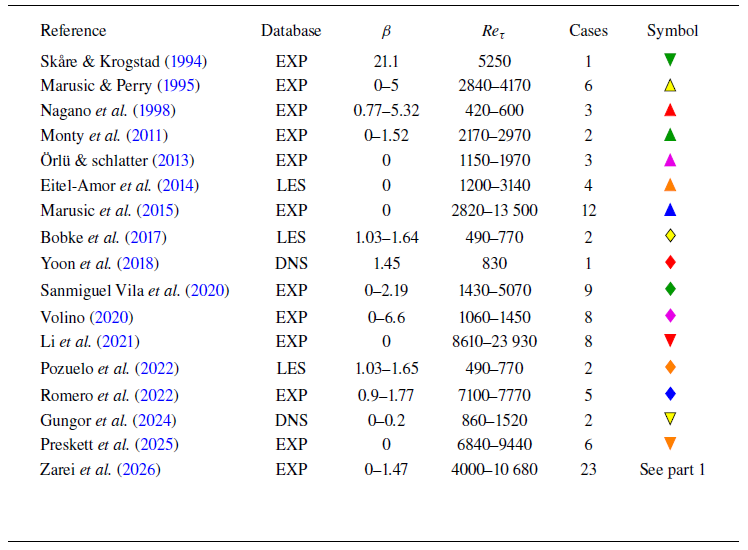

 Reτ

 CHw
 zc+
 Π
 Reτ=5000

 Reτ
 Reτ
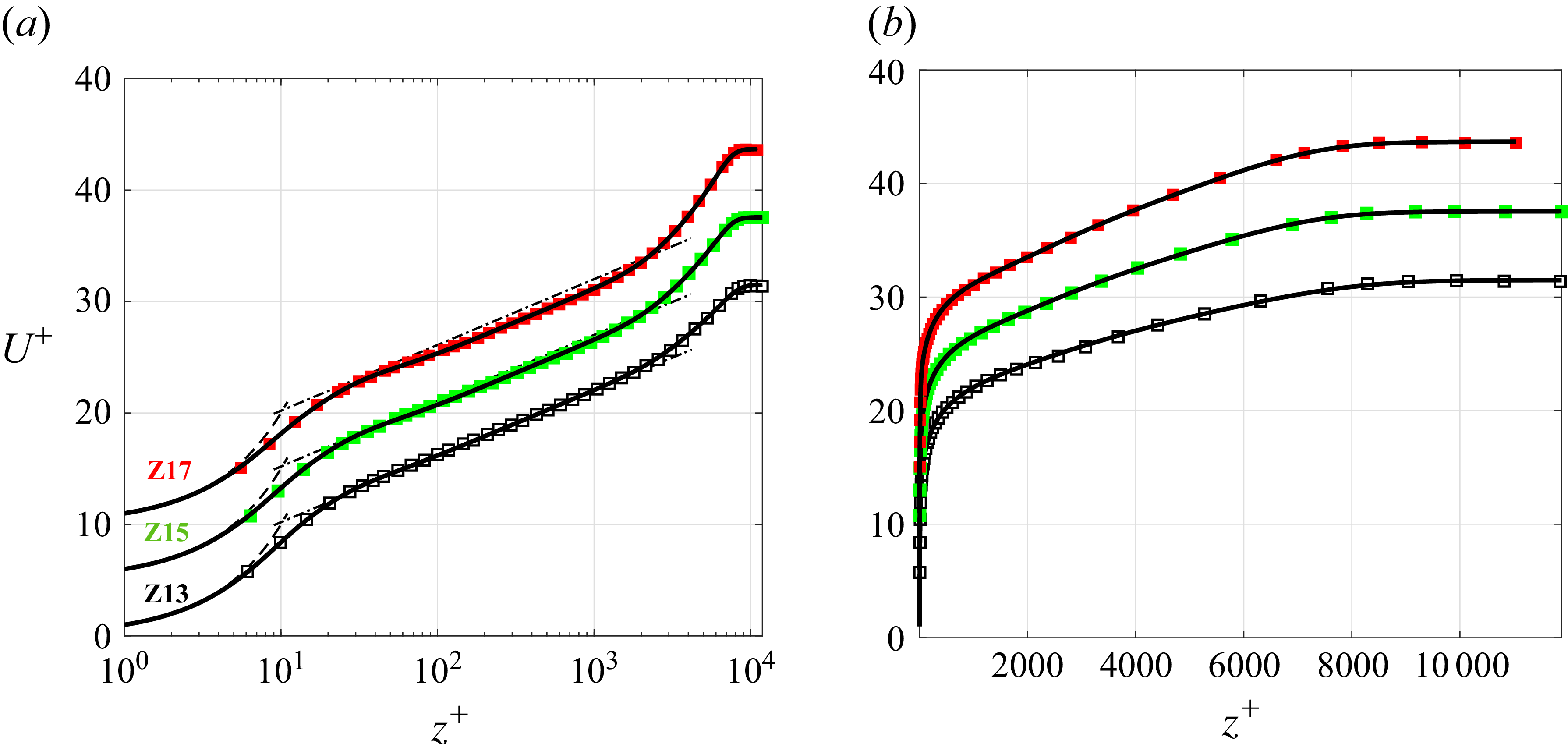
 Reτ


 δ

 zc+
 β
 CHi
 Reτ

 zc+
 β
 Reτ
 β

 CHw
 CHi

 Uτ
 2Π/κ
 δ

 Uτ

 Reτ
 Reτ
 Reτ
 1/κ

 z+
 κ
 Reτ
 βeff


 Π
 zc+
 CHw
 CHi
 βeff
 ±
 Uref=30
 U∞=30
 α=
 ∘

 βeff

 CHw
 CHi


 Open access

