


Democratic governance usually entails a system of institutions working in tandem to construct policy. In most modern democracies, courts are an important element of those institutions. The microlevel processes that underlie the distinct functions of law-making institutions have been extensively studied, especially the particular forms of policy making that each institution undertakes. The way courts make policy, though, is different from other institutions because judicial policy is made through the resolution of discrete cases, one at a time, rather than through the articulation of globally applicable policies. This observation has served as a starting point for many theories of rule construction and judicial politics (e.g., Cameron Reference Cameron1993; Cameron, Segal, and Songer Reference Cameron, Segal and Songer2000; Carrubba and Clark Reference Carrubba and Clark2012; Friedman Reference Friedman2006; Kornhauser Reference Kornhauser1992a; Reference Kornhauser1992b; Lax Reference Lax2007).
That judicial policy is made via the resolution of individual cases is important in part because the rules judges construct are themselves bound up with the factual scenarios giving rise to the cases. Indeed, the deep interconnection between factual scenarios and legal rules is a problem inherent in common law adjudication (Stein Reference Stein1992), as it creates possible indeterminacy of the law in factually distinct cases and creates room for disputing the relevance of past decisions for resolving new cases. Further, the principles of precedent and stare decisis, underlying common law adjudication, require existing rules be respected and applied only in factually similar future cases (Levi Reference Levi1949). Yet the practical realities of the world mean that truly identical disputes rarely arise, and the fact-bound nature of judicial inquiry means that even higher-court judges themselves cannot be sure exactly how certain fact patterns should be resolved without observing those facts closely in the context of a real-world case.
This creates challenges at each level of the judicial hierarchy. For lower-level courts, the challenge is how to use precedent and doctrine in cases that are similar yet different to precedent and for which guidance of higher courts is absent. The predominant method in practice is to use analogy to reason from precedent to factually distinct cases (e.g., Sherwin Reference Sherwin1999; Sunstein Reference Sunstein1999), although how to reason appropriately is frustratingly vague, and the logical foundations of the practice unclear, facing a long-standing challenge from legal theorists concerned about practical limitations to analogical reasoning (e.g., Cross Reference Cross2003).
For higher-level, supervisory courts, the challenge is how to formulate doctrine to guide lower-level courts across the full spectrum of possible case facts from a relatively small sample of actual cases heard, and through judgments that are themselves inextricably interwoven with the facts of the specific case at hand (see also Ellison and Holden Reference Ellison and Holden2014; Jordan Reference JordanN.d.). In turn, this points to the deeper strategic problem of how the higher-level court uses its discretionary jurisdiction to select optimally which cases to hear. Unfortunately, most of the theoretical research on case selection has focused on nondoctrinal features of cases or features not directly related to these challenges (cf. Caldeira and Wright Reference Caldeira and Wright1988; McGuire Reference McGuire1994; Perry Reference Perry1991; Ulmer Reference Ulmer1972). Knowing how courts use the resolution of individual cases to learn about and communicate authoritative doctrine, however, is critical to understanding the normative position of those courts in a democratic polity.
In this article, we develop a model of judicial learning and communication that speaks directly to the problems of legal rule writing, judicial decision making, and case selection in the world of uncertainty. The central tension we investigate concerns the court’s uncertainty about how different factual scenarios will manifest and the challenge that presents for a superior court in picking cases through which to articulate its doctrine. Our model relaxes a core assumption of many models of legal rule-making: that judges can easily order case facts and simply need to articulate doctrine that instructs lower courts and external actors how to resolve future cases (e.g., Cameron Reference Cameron1993; Kornhauser Reference Kornhauser1992b ; Lax Reference Lax2007; Reference Lax2011). By contrast, we conceive of the mapping from case facts to legal outcomes as a complicated mapping about which the courts are uncertain. To do so, we adopt the technology of Brownian motion previously used to study complex policy in other contexts (Callander Reference Callander2008; Reference Callander2011). This representation captures the richness of the law in practice as case facts map in a nonlinear, and unknown, way to legal outcomes.
Our results demonstrate how this complex informational environment drives decision making at all levels of the judicial hierarchy. We show that, in our model, optimal adjudication by lower courts proceeds via analogical reasoning, thereby establishing a logical foundation underneath this widespread practice in legal reasoning. We turn then to the behavior of higher-level, law-finding courts and show how they optimally respond to the use of analogy by lower level courts. We establish why the law must be created case by case and demonstrate the limits of overarching legal rules. We describe what makes a case more or less useful when building a body of law and use this to characterize the properties of optimal case selection by the higher court. In contrast to conventional wisdom, we show that the case selected is almost surely neither the case that is the “closest call” with respect to which party should win nor the case that is most dissimilar from past precedents and thus the most novel. We then turn to aggregate characteristics of the law and show how the law evolves over time in a path-dependent fashion. This path dependence is marked by increases but never decreases in the complexity of law, legal carve-outs in adjudication, and an evolution of doctrine that is logical yet difficult to predict.
The remainder of the article proceeds as follows. We begin with a description and motivation of our conception of the legal environment. We relate the Brownian motion representation to other formal approaches to the study of legal uncertainty, as well as to previous applications of its use. We present our formal results on analogical reasoning in judicial decision making, optimal case selection, and the path dependence of the law and then discuss the empirical implications. We conclude by pointing to several loose ends and other opportunities for further exploration of the model and results.
MODELING THE LEGAL ENVIRONMENT
Facts and Legal Outcomes
The primary job of courts is to take cases, characterized by particular factual scenarios, and dispose of them into mutually exclusive dispositions, such as guilty or innocent, liable or not liable, etc. (e.g., Kornhauser Reference Kornhauser1992b ). This task is not as easy as it sounds. One particular difficulty is that the language of cases and facts is different from the language of the law. To take a stylized example on which we rely throughout, consider search and seizure law. The Constitution prohibits “unreasonable” searches. Thus, the dimension along which judges must evaluate searches is their reasonableness, which can be thought of as a “legal fact.” However, cases are characterized by real-world facts, such as the location of the search, the circumstances under which it took place, the extent of the search, etc. (This distinction between real-world and legal facts has been emphasized by Friedman (Reference Friedman2006)) Exactly what constellations of real-world facts constitute unreasonable searches is a primary challenge for courts seeking to apply the law and is the source of complexity we study.
Put most simply, judges may be able to roughly order cases ex ante along a dimension of real-world facts, but there exists considerable uncertainty in the mind of an open-minded judge about what she would conclude about the reasonableness of a search until she actually reviews a case entailing such a search.Footnote 1 Thus, a primary source of uncertainty for judges, and a challenge for the judicial process, is distilling the relevant real-world facts of a case and translating them into a legal outcome.
It is this rich uncertainty that the Brownian motion representation is intended to capture. To be concrete, consider the setting familiar from the case-space approach to judicial decision making (e.g., Cameron Reference Cameron1993; Kornhauser Reference Kornhauser1992b ), in which case facts and judicial outcomes are represented spatially. In this model, judges choose partitionings to divide the fact space into a dichotomous “disposition space.” This model is depicted in the bottom panel of Figure 1. To continue the search-and-seizure example, the x axis in this figure represents the “intrusiveness” of a search, and the partitioning is between searches a judge finds acceptable and those she finds too intrusive. Implicitly, the model assumes judges can ex ante perfectly order all searches along the intrusiveness dimension, such that the distinction between real-world facts and legal facts plays no role.
Depictions of the Mapping from Real-World Facts to Legal Outcomes (top two panels) and Depiction of Standard Case-Space Model (bottom panel)

In contrast, our model assumes that judges can ex ante only roughly order cases according to real-world facts. Consider the top two panels of Figure 1. Here, each point along the x axes corresponds to a particular set of real-world case facts. More similar cases, from the court’s ex ante perspective, are closer in the space and dissimilar cases more distant. Legal facts are distinct and are represented on the vertical axes. For the sake of clarity—and as legal facts map directly into a judge’s preferences—we refer to the vertical axis as “legal outcomes.” The higher an outcome is on the axis the less “intrusive” is the search.
Judges observe real world facts but possess preferences over legal outcomes—the level of intrusiveness—rather than the real-world facts themselves. Each judge possesses a threshold in this space that distinguishes searches she prefers to “Permit” from those she prefers to “Exclude.” A judge with a threshold of zero prefers to rule Permit for outcomes above zero and Exclude otherwise. Outcomes close to zero correspond to “close calls” whereas those distant from zero are “easy cases” or, more colorfully, “slam dunks.”
The challenge for judges is to translate real-world facts into legal outcomes. Formally, there is a mapping that connects the two dimensions, such that for each set of case facts there is a corresponding legal outcome. This mapping may be a straight line, as in the top left panel of Figure 1, it may be a richer, non-monotonic mapping such as the realized path of a Brownian motion, as depicted in the top right panel, or it may be one of many other possibilities.
When this mapping is known, judicial decision making is involved but not particularly difficult. For any particular case facts, regardless of the mapping realized, the court can simply identify the corresponding legal outcome and determine the correct judgment. In this way, the model collapses to the canonical case-space model as the distinction between case facts and legal facts is rendered unimportant. Our interest is when the courts do not know the full mapping and this distinction is important. Courts, in practice, can never know the full mapping and may, in fact, know only a few points. In this case, the judicial task is substantially more complicated. Facing uncertainty about the translation of case facts into legal outcomes, how courts adjudicate the full range of cases is far from clear.
Learning about Legal Outcomes
Before delving into the details of this uncertainty, it is necessary to first establish how courts learn about the mapping. In practice, the difficulty in translating case facts into outcomes has led to specialization between courts and the creation of a hierarchy across them (e.g., Kornhauser Reference Kornhauser1995). Lower level courts specialize in the collection of facts—and are known as fact-finding courts—but do not possess the capability to independently interpret these facts, instead relying on the guidance of more expert courts. Above them in the hierarchy are expert courts—known as law-finding courts—that can both see facts (when they hear cases) and translate them into legal outcomes.Footnote 2
Our model considers both types of courts. “Law-finding,” or “Higher,” Courts are able to observe facts and to learn the legal outcomes, but have limited resources to hear cases. On the other hand, “fact-finding,” or “Lower,” courts are only capable of distilling facts; they cannot translate them into legal outcomes.Footnote 3 Fact-finding courts can, however, observe the legal outcomes from past cases the law-finding court has heard; that is, whenever the law-finding court hears a case, it establishes a precedent. Note this assumption contrasts with recent models in which the superior court is able to learn about the law from lower courts (e.g., Beim Reference Beim2015; Clark and Kastellec Reference Clark and Kastellec2013); here, learning is a strictly top-down process. Because law-finding courts cannot hear all cases, fact-finding courts must do the bulk of the judicial work, despite their inability to discern the legal outcomes for factually distinct new cases. In this sense, our model is similar to past models of law-building in which supervisory courts seek to use precedent to instruct lower-level courts that seek to apply, potentially imperfectly, the Higher Court’s instructions (e.g., Bueno de Mesquita and Stephenson Reference Bueno de Mesquita and Stephenson2002; Ellison and Holden Reference Ellison and Holden2014); the distinction is that in those models law-finding courts are assumed to have perfect knowledge and imperfect communication capacity. We assume, instead, perfect communication capacity but imperfect knowledge.
To see how a fact-finding court may reason from precedent, suppose that the court has access to a single precedent, say at point (0, ψ(0)) in the top two panels of Figure 1.Footnote 4 Now consider a fact-finding court using that precedent to resolve a new, distinct case, say at case facts p. While the precedent may offer some guidance on p, we would not expect it to be necessarily determinative. This is where the nature of the mapping becomes important. The simplest, and canonical, approach is to suppose that the mapping is linear, as in the top-left panel. Doing so, however, implies that the power of precedent is overwhelming and the fact-finding court’s problem trivial. From the single precedent, and knowledge that the mapping is linear, fact-finding judges would be able to infer the complete mapping and from this determine precisely the correct judgment for the case facts p and, indeed, for any other possible case facts, regardless of how far they may be from the precedent.Footnote 5 Such a simplification masks the very complexity that makes the judicial process so difficult. Indeed, the very distinction between fact-finding and law-finding courts suggests it is unreasonable to assume that a fact-finding court that cannot see the law directly itself, can nevertheless infer the correct judgment for all cases from one, or even a few precedents, regardless of how dissimilar the cases may be.
The nature of this problem can be understood by stepping back and examining how courts draw inferences and learn under uncertainty. Courts learn by combining two types of knowledge: practical and theoretical. Practical knowledge comes from precedent, from the experience of a particular case; theoretical knowledge concerns how cases and their outcomes relate to each other. The problem with the linear mapping is that it endows the courts with an excess of theoretical knowledge, so much so that, as we just saw, the addition of even the minimal amount of experience (of precedent) is sufficient to fully identify the legal environment. Even in models that relax the notion that a single precedent can perfectly inform the resolution of all future cases, the assumption of a linear mapping endows precedent with an extraordinary amount of information for future cases (e.g., Baker and Mezzetti Reference Baker and Mezzetti2012).
A more reasonable—and realistic—presumption is that the relationship between case facts and outcomes is less regular. Nearby cases should be more likely to produce nearby outcomes and, thus, precedent should be instructive, but not determinative, when combined with theoretical knowledge. As Hume (Reference Hume1748) famously argued in his treatise on induction, “From causes which appear similar we expect similar effects.” The unwritten complement of this statement is that dissimilar causes should yield dissimilar, or at least less similar, effects.
The Brownian motion representation captures these desiderata concisely, and in so doing it provides a simple parameterization of the degree to which precedent can be applied across other cases. As is evident from the top-right panel of Figure 1, the Brownian motion mapping is highly nonlinear, with ups and downs that capture the vagaries and uncertainties of judicial decision making in the real world. This allows for the possibility of “carve-outs” in the law and legal rules that do not have a single cut-point that divides cases monotonically along the factual dimension (thus, we are not limited to the kinds of rules Lax (Reference Lax2007) refers to as proper rules).
The Brownian motion contains two components, defined by the drift and the variance. The drift is the expected rate at which the mapping changes, and is depicted by the dashed line in Figure 1. This constitutes the predictable part of the law. Judges know that case facts to the right are more likely—but not certain—to lead to lower outcomes (for drift that is negative). The variance is the unpredictable component of the law. It is the variance that leads to the ups and downs, the unexpected carve-outs and exceptions that mark law-making in practice. The combination of unpredictable variance with predictable linear drift implies that the Brownian motion can be seen as a generalization of the linear mapping of the left panel, extending it to capture the vagaries and richness of the legal decision making in practice. Put differently, the Brownian motion captures the notion that while judges may be able to roughly order hypothetical cases ex ante with respect to their associated legal outcomes, there is often some consequential nuance that the law-finding judges can only learn by hearing the case itself.
To capture this richness, we presume throughout the remainder of the article that the mapping from real world facts to legal outcomes is the realized path of a Brownian motion with drift, μ < 0 and variance σ2. The courts know these parameters and at least one point in the mapping, what we think of as a case of first instance that opens up the legal area, and which we denote by (0, ψ(0)). As our interest is how courts grapple, reason, learn, and communicate in a complicated legal environment, we set aside the questions of preference differences and incentive constraints. Specifically, we suppose that all courts share the same preferences and the same threshold at zero that demarcates between legal outcomes that are best adjudicated Permit and Exclude. This is known as the “team” model of the judiciary (e.g., Kornhauser Reference Kornhauser1995). As a result, any inefficiency that arises in this setting is due exclusively to the informational challenges of the complex environment.Footnote 6
JUDICIAL DECISION MAKING IN A COMPLICATED WORLD
In a complicated world that is partially yet not perfectly predictable, how do Lower Courts arrive at judgments? For cases that match precedent, the answer is trivial: The Court follows the Higher Court’s judgment. Practical knowledge overwhelms theoretical knowledge for these cases. The correct judgment has been identified by the Higher Court, and it is immediate that the Lower Court finds it optimal to follow this judgment. However, this logic holds only when case facts exactly match precedent. Both in our formalization and in the real world of adjudication, identical cases have zero probability of occurring. The question of interest then becomes: How do the Lower Courts adjudicate in the gaps?
To answer this question, we must first define what the courts are trying to achieve; that is, their preferences over case dispositions. We then turn to how the courts reason and make decisions.
Preferences
A judge’s objective is to render correct decisions. However, some correct decisions matter more than others. For instance, excluding an egregious search is more valuable than excluding a search that is marginal. Conversely, making a mistake on what should be a “slam dunk” case is more costly than on a “close call.” Formally, this means that judges benefit more from correct decisions that are well over their decision threshold—the threshold of doubt—and suffer more when they get these decisions wrong. Similar to Beim, Hirsch, and Kastellec (Reference Beim, Hirsch and Kastellec2014), we formalize this relationship linearly. For a judge with a decision threshold of zero, such that she prefers the judgment ”Permit” if ψ(p) ⩾ 0 and the judgment ”Exclude” if ψ(p) < 0, utility for case facts
 $p\in \mathbb {R}$
is
 $$\begin{equation*}
u\left( p\right) =\left\lbrace \begin{array}{l@l}\left|\psi\, \left( p\right) \right|& \text{if}\ \text{correct decision made,} \\[4pt]
-\left|\psi\, \left( p\right) \right|& \text{if}\ \text{incorrect decision made.} \end{array} \right.
\end{equation*}$$
In a team setting, as we consider, all judges share this same utility function and the same decision threshold of zero.
Judicial Reasoning
Before Lower Court judges can come to a decision on a set of case facts, they must first form beliefs over the likelihood as to which outcome may be the correct one. These beliefs are imprecise for case facts that have yet to be heard, as they would be in practice. To reason from what knowledge they do have and arrive at an optimal, if imperfect, judgment, judges combine the practical knowledge from experience with their theoretical understanding of the legal environment. The importance of each type of knowledge depends on the type of case facts under consideration. Borrowing the terminology of Schumpeter (Reference Schumpeter1934), a case can be one of either exploitation or exploration. (We summarize various typologies of cases we use throughout the article in Table 1.) A case of exploitation lies within the existing body of legal knowledge. A case of exploration, on the other hand, lies outside these bounds in new legal territory. The right-side panel of Figure 2 depicts three precedents at zero, pl , and pr . Cases of exploitation are those between zero and pl , and between pl and pr . Cases of exploration are all cases to the right of pr and to the left of zero. In the left-side panel only the case of first instance is known and all cases are exploratory.
Example Brownian Bridges.

Selected Terminological Definitions

Exploitative cases provide the judges with more practical guidance than do cases of exploration, so much so that the practical knowledge dominates. Formally, taking cases between pl and pr as example, beliefs for all p ∈ (pl , pr ) are normally distributed, with
 $$\begin{eqnarray}
\mathbb {E}\left[ \psi\, \left( p\right) \right] &=&\psi\, \left( p_{l}\right) +\frac{p-p_{l}}{p_{r}-p_{l}}\left( \psi\, \left( p_{r}\right) -\psi\, \left( p_{l}\right) \right) \text{,}
\end{eqnarray}$$
 $$\begin{eqnarray}
var\left[ \psi\, \left( p\right) \right] &=&\frac{\left( p-p_{l}\right) \left( p_{r}-p\right) }{p_{r}-p_{l}}\sigma ^{2}\text{.}
\end{eqnarray}$$
The expected outcome for an exploitative case is given by Equation (1) and the variance by Equation (2). The expected outcome is more easily seen graphically as it is simply the straight line between the nearest precedent in either direction; this is depicted in Figure 2 by the dashed lines that join the precedents. Notably, the judge uses only knowledge of the nearest precedent in either direction, discarding all other information.
The variance of beliefs varies according to how novel a set of case facts is. Uncertainty reaches a peak exactly midway between the neighboring precedents (pl and pr ) and approaches zero as a case becomes more similar to either precedent. This captures the idea that uncertainty is highest the more novel is a set of case facts. In Figure 2, the size of uncertainty is represented by the dotted lines between the precedents.
For reasoning over exploitative cases, practical knowing is ascendant. Theoretical knowledge plays no role in the formulation of expected outcomes as the drift and variance terms, μ and σ2, are absent from the judge’s beliefs. The only knowledge that matters is the nearest precedents, the outcomes they produce, and the distance between them in case fact space. The variance term, σ2, does appear in the variance of beliefs in Equation (2), parametrizing the “noisiness” or complexity of the environment.
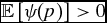
The expected outcome in Equation (1) represents the judge’s best guess as to the true outcome. She may be wrong but law in practice demands that she issue a judgment despite her uncertainty. The judge arrives at her best guess by reasoning by analogy from previous cases, independent of her theoretical knowledge of the environment. Our first result establishes that it is optimal for the judge to follow this best guess in making her ruling. It is optimal, therefore, for the judge to adjudicate via analogical reasoning.Footnote 7
Property 1 For exploitative cases, fact-finding courts reason from analogy by linearly weighting the nearest precedent in either direction. If p
1 and p
2 are the nearest precedents to the left and right, respectively, then for p ∈ [p
1, p
2], the optimal ruling is Permit if
 $\mathbb {E}\left[ \psi\, \left( p\right) \right] >0$
, and Exclude otherwise.
Of interest is not only that judges reason by analogy in formulating rulings, but how they so reason. The method in Property 1 matches features of practice. Substantively, a judge selects the most similar precedent in either direction, ignoring all other precedent. This property is similar to the judicial practice of selecting on-point (or, “controlling”) precedents and applying some sort of balancing test to them in forming an opinion.
The behavior underlying Property 1 follows from the mathematics of the Brownian motion and Bayesian updating. The import of our result is to show that this optimizing behavior matches analogical reasoning as used in practice. It establishes that analogical reasoning is not only an effective response to a complicated legal environment, but that it is an appropriate and even optimal method for dealing with substantial uncertainty.
Exploratory cases cannot apply the same method of reasoning as a second on-point precedent is simply not available. For these cases, the judges must lean more on their theoretical knowledge of the environment, combining it with the practical knowledge they do have. For cases on the right flank, p > pr , beliefs are normally distributed with
 $$\begin{eqnarray}
\mathbb {E}\left[ \psi\, \left( p\right) \right] &=&\psi\, \left( p_{r}\right) +\mu \left( p-p_{r}\right) \text{,}
\end{eqnarray}$$
 $$\begin{eqnarray}
var\left[ \psi\, \left( p\right) \right] &=&\left|p-p_{r}\right|\sigma ^{2}\text{.}
\end{eqnarray}$$
The expected outcome is given by Equation (3) and variance by Equation (4). Uncertainty is again parametrized by σ2, with uncertainty higher the more novel is a set of case facts, and depicted by the dotted lines in the figure. In contrast to exploitative cases, uncertainty increases without bound and can become arbitrarily large as there is no on-point precedent to the right to anchor knowledge.
A second notable difference with exploratory cases is the presence of the drift term μ in Equation (3). This implies that judges require theoretical knowledge of the underlying legal environment to effectively form beliefs for exploratory cases. Judges use the right-most precedent to anchor beliefs, and apply their theoretical knowledge to guide expectations, with the drift parameter μ measuring the rate at which the expected outcome changes. This is depicted in Figure 2 by the dashed line that begins at point (pr , ψ(pr )) and decrease to the right of pr at rate μ; the dashed line departing to the left of the precedent at 0 represents the analogous beliefs on the left flank.
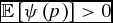
The expected outcome in Equation (3) again reflects the judge’s best guess as to the true outcome, and again it is optimal for the judge to follow this best guess in rendering judgement. This is formalized by Property 2.
Property 2 For exploratory cases, fact-finding courts reason from analogy in combination with theoretical knowledge of the legal environment. If pr
is the right-most precedent, then for p > pr
, the optimal ruling is Permit if
 $\mathbb {E}\left[ \psi\,\; \left( p\right) \right] >0$
, and Exclude otherwise.
As for exploitative cases, judges use the experience of precedent to anchor their reasoning, but, without an anchor to pin down one of the sides, theoretical knowledge is required to extrapolate effectively. This need resonates with practice as more novel cases are generally considered to be harder and to require more legal expertise. We have assumed that the Lower Courts possess the necessary theoretical knowledge, although in practice this may not be the case; we take up this question in the concluding discussion and explore what expertise differences might mean for communication across the judicial hierarchy and the formation of doctrine.
With the behavior of the Lower Courts in hand, we turn now to the question of how law-finding courts allocate their efforts and attention in a world in which reasoning by analogy is the optimal modus operandi of Lower Courts. Should the Higher Court hear only exploratory cases? Should it aim for cases with the highest variance? Or cases in which the Lower Courts are most likely to be wrong in their judgments? We answer these questions, among others, in what follows.
CASE SELECTION AND THE PATH OF THE LAW
For law-finding courts the question of judicial decision making is not so much about forming judgments on particular cases—as the court can see the true outcome and knows the correct judgment—rather it is about which case to hear given its limited resources. In this section, we develop a model of a judicial hierarchy and explore optimal case selection of a law-finding court and the path of law this generates.
A Model of a Judicial Hierarchy
The legal hierarchy has two sets of players. At the top is a single, law-finding Higher Court. At the beginning of each period t, where t = 1, 2, 3, . . ., the Higher Court has the choice to hear a single case at cost c > 0. Upon hearing a new case pt , the Higher Court observes the true outcome, ψ(pt ), reveals it to the world, and issues a judgment of either Permit or Exclude, denoted J(pt ) ∈ {P, E}. The Higher Court’s judgment threshold is zero; thus, it is trivially obvious that the optimal judgment is P for permit if the outcome ψ(pt ) ⩾ 0 and E otherwise. The newly discovered point in the mapping, (pt , ψ(pt )), becomes a new precedent. The set of precedents then becomes ht = {(0, ψ(0)), (p 1, ψ(p 1)), (p 2, ψ(p 2)), . . ., (p t′, ψ(p t′))}, for t′ ⩽ t.
At the bottom of the hierarchy is a set of fact-finding Lower Courts. With the set of precedent, ht , in hand, these courts adjudicate by analogy as described in the previous section. The Lower Courts collectively hear a mass of cases each period according to the distribution f( · ) where, for simplicity, f is distributed uniformly over an interval that spans zero and is large.Footnote 8 As noted above, we assume a team model of the courts, and so all judges’ preferences are aligned, and the Lower Courts therefore also have an ideal threshold of zero. For simplicity, we further assume that the Higher Court seeks in each period to maximize the quality of legal decision making in that period, setting aside forward-looking considerations, which only complicate our analysis while reinforcing the conclusions we draw.Footnote 9
In our model, as in the most judicial hierarchies, the logic is that there exists a highly capable Higher Court that is resource constrained. Picking up the workload is a set of less talented but nevertheless logical fact-finding courts. These courts combine precedent and theoretical knowledge as best they can but, inevitably, these efforts will be imperfect and impact the large number of cases that appear on their dockets. The challenge for the Higher Court is to determine when it is appropriate to hear a new case and, if so, which case will most assist and improve the decision making of the Lower Courts.
The Value of Certiorari
To consider how the Higher Court chooses which cases to hear, we must first establish how a new precedent improves Lower Court decision making. Although reasoning by analogy is optimal, it is imperfect in the judgments it produces. The expected outcome is just that, an expectation, and with positive variance (and a normal distribution) it is always possible, however remotely, that the true outcome lies on the opposite side of zero and the judgment induced by the expected outcome is incorrect. Adding a new precedent can reduce the probability of such errors — indeed, that is the point—but to understand how valuable this reduction is, we must first understand how errors impact the utility of the courts.
The answer is surprisingly subtle. Consider the Lower Courts’ expected utility for case facts p and expected outcome
 $\mathbb {E}\left[ \psi\,\; \left( p\right) \right]$
. When a fact-finding court issues the judgment Permit, expected utility is
 $$\begin{eqnarray*}
\mathbb {E}u\left( \text{Permit}|p,\mathbb {E}\left[ \psi\, \left( p\right) \right] \right) &=&\int _{0}^{\infty }\left|z \right|\phi \left( z\right) dz\\
&&-\,\int _{-\infty }^{0}\left|z \right|\phi \left( z\right) dz,
\end{eqnarray*}$$
where z represents possible values of ψ(p) and ϕ(z) is the density of the normal distribution of mean
 $\mathbb {E}\left[ \psi\,\; \left( p\right) \right]$
and variance var(ψ(p)), with variance given by Equation (2) or (4) depending on the type of case. The first term on the right-hand side is the set of outcomes for which the decision to Permit is correct (values of ψ(p) between 0 and ∞), whereas the second term is the outcomes for which this decision is incorrect (values of ψ(p) between − ∞ and 0). Rearranging, we have
 $$\begin{eqnarray}
&&\mathbb {E}u\left( \text{Permit}|p,\mathbb {E}\left[\psi\, \left( p\right) \right]\right) \nonumber \\
&&\quad=\int _{0}^{\infty } z \phi \left( z\right) dz-\int _{-\infty }^{0}-z \phi \left( z\right) dz \nonumber \\
&&\quad=\int _{0}^{\infty } z \phi \left( z\right) dz+\int _{-\infty }^{0} z \phi \left( z\right) dz \nonumber \\
&&\quad=\int _{-\infty }^{\infty } z \phi \left( z\right) dz \nonumber \\
&&\quad=\mathbb {E}\left[ \psi\, \left( p\right) \right].
\end{eqnarray}$$
Expected utility is simply the utility should the expected legal outcome be the true legal outcome. Surprisingly, variance plays no role; consequently, expected utility is entirely independent of the complexity of the legal environment.
This property presents a perplexing problem for the Higher Court. If expected utility does not depend on variance and uncertainty, what role is left for the Higher Court’s ability to reduce variance? To answer this question, we need to delve more deeply into the logic of Equation (5). The logic is easiest to understand visually, as in Figure 3. Consider case facts p in the left panel, with nearest precedents pl
and pr
and expected legal outcome
 $\mathbb {E}\left[ \psi\,\; \left(p\right) \right]$
. Actual utility will match expected utility only in the unlikely event that the realization of ψ(p) matches the expectation precisely. For all other possible realizations, actual utility will either be higher or lower. (The following logic holds also when the precedents give opposing judgments, as in the right-side panel.)
The Source of Value

Consider then an arbitrary pair of possible legal outcomes, l 1 and u 1, that are equally distant from the expected legal outcome, as depicted. Utility is lower than expected if l 1 is the realized legal outcome, whereas utility is higher than expected if u 1 is realized. Because these possibilities are equidistant from expectation they counterbalance each other and their net effect on expected utility is zero (as they are of equal probability due to symmetry of the normal distribution).Footnote 10 This same logic holds for all such pairs, and expected utility is given exactly by the utility of the expected legal outcome.
To see the role for new precedent, observe that the above logic holds even for the pair u 2 and l 2. The lower outcome is interesting as for this outcome the judgment of the Lower Court is in error. The correct judgment for a legal outcome below zero is Exclude, yet the decision of the Lower Court, based on analogy, is to Permit. Thus, the utility of the Lower Court’s decision given this legal outcome is negative. The possibility of error does not upset the logic of expected utility described above, but it does matter to the Higher Court. It matters because, by hearing a new case and observing the true legal outcome, the Higher Court can rectify error and increase utility. The benefit of these correctives is directly proportional to how often judgments are wrong and how serious are the mistakes made. Both of these factors strictly increase in σ2, the complexity of the legal environment. All else equal, therefore, for case facts p the value to the Higher Court of granting certiorari is strictly increasing in complexity.
Optimal Case Selection
The preceding discussion suggests that, to have maximum impact, the Higher Court should seek out the case with the highest variance, what we refer to as outcome uncertainty. After all, whenever the court hears a case, uncertainty for that case reduces to zero (as the true legal outcome is revealed), and thus the greatest reduction would be for the case that begins with the highest uncertainty. Although this logic accords with the view that courts should remove legal uncertainty, it affords a too narrow view of how best to go about this task.
One element missing from this logic is how meaningful is the uncertainty that is removed. It is possible for a case to have high outcome uncertainty but for this uncertainty to have little import on the correctness of the judgment. For instance, if most of the uncertainty is concentrated on one side of zero (on one side of the judgment threshold) then it is of little importance as the judgment of the court remains almost surely correct. To illustrate, let us return to the search and seizure example. There may be a new search involving a factual situation that is very far outside of the bounds of factual scenarios previously considered, for example using some powerful type of imaging technology that allows police to see inside one’s home. In this instance, the Court may be uncertain about exactly how intrusive that search is but have little uncertainty about whether the level of intrusiveness is enough that it would prefer to exclude such searches. On the other hand, consider a type of search that is “between” past cases but presents a close call to the Court. For example, suppose a technology that captures signals coming from one’s cell phone and decode them to read text messages. Past precedent says that the police require a warrant to listen to phone conversations but that they do not need a warrant to use infrared to image the interior of a house using the pattern of heat being emitted. This new hypothetical technology seems to be somewhere in between, and a court might have a great deal of uncertainty about which side of the threshold of permissible searches this case falls on, independent of how much uncertainty it has about the level of intrusiveness.
Thus, of relevance for case selection is a second measure of uncertainty—what we refer to as error uncertainty—that captures the probability that a judgment reasoned from analogy is incorrect. The size of error uncertainty depends on how much probability mass lies on the opposite side of zero to the expected outcome. This is maximized at exactly one half when the uncertainty is equally distributed about the zero threshold. In this event the correct judgment is equally likely to be Exclude or Permit, and any judgment issued by the Lower Courts is as likely to be wrong as it is right.
A vein of thought in legal practice is that law-finding courts should seek out and hear cases that maximize error uncertainty; that is, to hear cases for which the legal outcome is most uncertain. However, for the same reason that outcome uncertainty is not the court’s only concern, neither is error uncertainty fully determinative of optimal behavior. It may be that the case that maximizes error uncertainty has very low uncertainty overall. In such a situation it is a coin toss whether a judgment is correct or not, yet the errors induced are not very costly (as realized legal outcomes are clustered around zero). The value to a case of being heard by the Higher Court must balance the dueling effects of outcome uncertainty and error uncertainty. The most valuable case lies somewhere between these extremes and is the one that maximizes the expected cost of errors.
Yet even this logic is incomplete, for the value of the Higher Court hearing a case is not limited to only that case. Because similar cases should lead to similar legal outcomes, as observed by Hume (Reference Hume1748), the Higher Court hearing a case not only removes uncertainty for that case, it impacts uncertainty for many similar, neighboring cases. In selecting a case, the Higher Court must allow for this broader impact. Indeed, given that a single case is unlikely to be repeated, whereas the neighborhood of cases facts will surely recur, the overwhelming impact of hearing a case is its impact on other cases rather than the case itself. (Formally, relative to the continuum of case facts, the mass of a single case is zero.) This logic resonates with the conventional wisdom in legal circles that while Lower Courts focus on the cases in front of them, Higher Courts adopt a “big picture” approach in adjudication and, in particular, case selection.
The trade-offs when considering broader impact are the same as for a single case. The court seeks to minimize judicial errors by the Lower Courts and to minimize those errors that are particularly costly. We consider first the choice over standard and exploitative cases. An exploitative case is standard when the on-point precedents give opposing judgments. In this range, therefore, the best judgment is far from clear and requires a balancing of precedent, what one might think of as the standard work of courts. Standard exploitative cases are depicted in Figure 4 for case facts between pl and pr .
Cases the Higher Court will Hear Among Exploitative and Standard Cases

For standard exploitative cases, the case that maximizes error uncertainty is easy to identify. It is the case for which the expected outcome is exactly zero, as then half the uncertainty is above zero and half below. It is given by case facts p in Figure 4. For this case, the correct judgment is as likely to be Permit as it is to be Exclude and error uncertainty attains the maximum possible value of one half. The case that maximizes outcome uncertainty is also well defined and readily identified. It is the case that is exactly equidistant from the on-point precedents, as can be seen Equation (2); the maximum outcome uncertainty is marked by case facts
 $\frac{p_r+p_l}{2}$
in the figure.
Proposition 1 establishes that one of these cases is selected only when they coincide—in which case both are selected—and that this is an exceedingly rare event (in fact, it is a zero probability event). In all other situations, the Higher Court selects neither of these benchmark cases. Rather, it trades off between them and chooses a case that lies strictly between them.
Proposition 1 From a set of standard exploitative cases, the Higher Court optimally hears a case that lies strictly between the cases of maximum error and maximum outcome uncertainty. When these cases coincide, that is the case that is heard. Formally, for the set of cases p ∈ (pl , pr ), where ψ(pl ) > 0 and ψ(pr ) < 0, the optimal case facts for the Higher Court to hear, p*, satisfy the following: If
-
(i) ψ(pl ) < |ψ(pr )|, then |p* − pl | < |pr − p*| and
 $\mathbb {E}\left[\psi\,\; \left( p^{*}\right)\right] <0$
;
-
(ii) ψ(pl ) > |ψ(pr )|, then |p* − pl | > |pr − p*| and
$\mathbb {E}\left[\psi\,\; \left( p^{*}\right)\right] >0$
; -
(iii) ψ(pl ) = |ψ(pr )|, then |p* − pl | = |pr − p*| and
$\mathbb {E}\left[\psi\,\; \left( p^{*}\right)\right] =0$
.



The coincidence of maximum outcome and maximum error uncertainty occurs when ψ(pl ) = |ψ(pr )|, as captured by (iii) in the proposition. As can be seen, this requires the on-point precedents to be exactly equidistant from zero, an event that is possible but that has zero probability of occurring. The more typical situation is depicted in Figure 4, which represents (i) in the proposition. For it and the situation in (ii), the court seeks out a middle ground. The set of possible cases may be broad or it may be narrow, with the width depending on the particular history of precedent that emerges. Regardless, the case chosen is closer to the on-point precedent that has outcome closer to zero, but has an expected outcome that matches the on-point precedent further from zero.
This implies that the case selected has a legal outcome that is already “known,” at least in the sense that one legal outcome is more likely than the other, possibly significantly so. Choosing such cases is common in practice, yet has often seemed puzzling. Our model provides a natural explanation for such case selection. Although the correct judgment for the case in hand may be in little doubt, the actual outcome may remain highly uncertain, and the interdependence of legal outcomes across cases implies that this information is nevertheless valuable. By confirming the correct judgment, and revealing the true outcome, for the “known” case, the Higher Court may provide significant benefit across a broad swathe of other cases, cases that the Higher Court itself does not have time to hear.
Similar logic applies for selection among other types of cases. Proposition 2 deals with nonstandard exploitative cases. These cases lie between two precedents in which the precedents have matching judgments. They are nonstandard in the sense that to either side, precedent guides the Lower Courts to the same destination, and an observer may wonder where the legal uncertainty lies. Yet, as we saw earlier, it remains possible that cases between these precedents yield a different judgment, and this gives value to hearing a non-standard case. Nonstandard exploitative cases can be seen in Figure 4 in the interval between case facts zero and pl . In this situation the case of maximum outcome uncertainty is again at exactly the halfway point of the interval. However, there is no case that attains an error uncertainty of one half. Nevertheless, error uncertainty is biased toward one end of the set of possible cases—toward the precedent without outcome closer to zero—and the case chosen must always come from this subset. Again, for this choice to correspond to the case of maximum outcome uncertainty requires the on-point precedents to be exactly equal, a zero probability event.
Proposition 2 From a set of nonstandard exploitative cases, the Higher Court optimally hears a case that lies strictly between the cases of maximum error and maximum outcome uncertainty. When these cases coincide, that is the case that is heard. Formally, for the set of cases p ∈ (pl , pr ), where ψ(pl ) > 0 and ψ(pr ) > 0, the optimal case facts for the Higher Court to hear, p*, satisfy the following: If
-
(i) ψ(pl ) < ψ(pr ), then |p* − pl | < |pr − p*| and
$\mathbb {E}\left[\psi\,\; \left( p^{*}\right)\right] >0$
; -
(ii) ψ(pl ) > ψ(pr ): then |p* − pl | > |pr − p*| and
$\mathbb {E}\left[\psi\,\; \left( p^{*}\right)\right] >0$
; -
(iii) ψ(pl ) = ψ(pr ): then |p* − pl | = |pr − p*| and
$\mathbb {E}\left[\psi\,\; \left( p^{*}\right)\right] >0.$



Our final proposition for this section turns to exploratory standard cases.Footnote 11 For these cases, there are not opposing judgments from the on-point precedents as there is only a single on-point precedent. These cases arise in the first period when an exploratory case is unavoidable, and will recur whenever the right-most precedent yields an outcome above zero (or the left-most precedent reveals an outcome below zero). For these cases, the line of expected legal outcome crosses zero. Thus, there exists a case with expected outcome of zero and a case of maximum error uncertainty does exist. There is, however, no case that maximizes outcome uncertainty as uncertainty increases without bound for cases further from precedent. Nevertheless, the logic of previous propositions carry over here. The court balances outcome and error uncertainty, such that the case chosen is bolder, and more exploratory, than the case of maximum error uncertainty.
Proposition 3 For the set of exploratory and standard cases p > pr
, where ψ(pr
) > 0, the optimal case facts for the Higher Court to hear, p*, is such that
 $\mathbb {E}\left[ \psi\,\; \left( p^{\ast }\right) \right] <0$
.
The balancing of uncertainties implies that the court explores so boldly that the expected legal outcome of the case heard is on the opposite side of zero from the on-point precedent, and, consequently, yields a different expected outcome. Thus, when the Higher Court decides to explore an area of cases, it does so boldly and with the intent of selecting a case that it expects to create a region of exploitative, standard cases that can pin down the law.
The logic of Higher Court case selection just described reinforces the importance of interdependencies across cases for all levels of the judicial hierarchy. The Lower Courts reason by analogy as legal outcomes are interdependent, and this same interdependence motivates the Higher Court to consider the broader impact of the cases it hears as, in turn, it knows the Lower Courts will reason by analogy from the precedent handed down. The power of our theorizing is to explain these twin behaviors and to expose the connection between them, providing a parsimonious theory of broad judicial behavior.
Legal Complexity, Doctrinal Complexity, and the Path of Law
We turn now from within-period case selection to what this means across time as precedent accumulates and the law evolves. A common and idealistic view is that the law evolves in a rational, thoughtful, and conservative way along a trajectory that perhaps slowly but inexorably converges on the truth and a complete understanding of the legal environment. Clashing against this view is the reality that judicial decision making in practice is seemingly much more haphazard, irregular, and ostensibly without reason. In this section, we demonstrate how to reconcile these perspectives. We show what the idealistic view omits as well as the truth that it captures.
First period behavior in our model is relatively straightforward. As prescribed by Proposition 3, when the Higher Court hears a new case, it hears one that boldly departs from the case of first instance. The value of hearing this case is increasing in outcome and error uncertainty so that, intuitively, the Higher Court is more likely to hear a case the more complex is the area of law. (We formalize and return to this result in Proposition 6 below.) What happens after this case is heard is more difficult to pin down. In each subsequent period, the judges will render judgments according to the optimizing behavior described herein. Yet, this behavior yields no discernible pattern in the types of cases heard.
To see this, suppose the legal outcome of the first case is similar to the legal outcome from the case of first instance; that is, ψ(p 1) is similar to ψ(0), as depicted in Figure 5. The court then has the choice in the second period to hear another exploratory case to the right of p 1, or it can backpedal and instead hear an exploitative nonstandard case between 0 and p 1. How the court resolves this choice depends on the exact values of the legal outcomes, the distance between precedents, and the underlying complexity of the legal area. As more and more precedents accumulate, the possibilities multiply and the richness of choice expands. Calculations reveal that no pattern appears in the sequence of cases, and it is possible for any type of case to follow any other type, depending on the legal outcomes realized (e.g., a standard exploitative case may be followed by another exploitative case or by an exploratory case, with each potentially standard or nonstandard).
Example of Cases the Higher Court can Consider as Precedent Accumulates

The upshot of this is that a rich path dependence emerges in the law. The cases elevated to the Higher Court depend not only on what was heard before but on the legal outcomes observed. This matches the reality of case selection in practice that follows no predictable sequence (at least in the medium to long run). Yet it shows that this apparent haphazardness is exactly what should emerge from rational, deliberate doctrinal choice by a capable court when the underlying legal environment is complex. The path dependence of the law leads to the accumulation of a rich and potentially large body of precedent, complicating the Lower Courts’ task. Keeping track of precedent imposes cognitive demands on the courts, demands that are relevant given the limited resources and demanding case loads faced by the Lower Courts.
Not all precedents are created equal, however, and it is possible to reduce this informational load without compromising the needs of the Lower Courts. The information essential to Lower Court decision making is knowing which case facts should be adjudicated one way and which case facts the other way. Although this knowledge is deduced from precedent, it can be defined directly in the space of case facts as a set of cut-points that delineate the appropriate judgments.Footnote 12 Significantly, the number of cut-points need not correspond to the number of precedents and, typically, will be smaller.Footnote 13 The more cut-points the more complicated is Lower Court decision making and this number can be taken as defining the complexity of legal doctrine.
Doctrinal complexity evolves more regularly than the law itself. It is possible that the number of cut-points remains constant for stretches of time. However, when complexity does change, it only changes in the direction of increasing complexity. Individual cases can provide more clarity, in the sense of more surely identifying where the legal mapping crosses the zero decision threshold, but, in our setting, they cannot reduce doctrinal complexity, which may account for why legal procedure is often so complicated. Individual cases, for all their other benefits, cannot cut through the complexity of doctrine and counter the relentless pressure toward greater complexity.Footnote 14
This observation raises the question of what causes complexity to increase and, equally importantly, what causes it to remain unchanged. The answer depends systematically on the types of cases that are heard. To see the possibilities, consider again Figure 5. In this situation the doctrinal complexity is one as the Lower Courts need only keep track of the single cut point at n 0.
Suppose, then, that the court hears a nonstandard case p between zero and p 1. Regardless of the legal outcome, the new precedent that is established separates the expected outcome line between zero and p 1 into two separate but continuous segments. If the legal outcome of p is u 1, u 2, l 1, or any legal outcome above zero, then the the expected outcome lines also remain above zero for all cases impacted. Consequently, despite the addition of a new precedent, the behavior of the Lower Courts remains unaffected. The courts need only continue to keep track of the single cut point at n 0 and doctrinal complexity is unchanged. This precedent, then, does now affect how the Lower Courts apply the law and so does not need to be considered when the Lower Court hears future cases.Footnote 15
On the other hand, if the legal outcome of p should be l 2, or any outcome below zero, the Lower Courts must pay attention and react. In this event, the new precedent not only affects how the Lower Courts adjudicate case facts p but it impacts how they adjudicate neighboring cases as well. As can be seen in Figure 5, the expected outcome lines cross the zero threshold, and do so at two distinct points, n 1 and n 2. The new cut-points create a carve-out in fact space; the Lower Courts rule Exclude for cases in the interval (n 1, n 2) and Permit to either side. This reflects an increase in doctrinal complexity and demonstrates the general property that when doctrinal complexity increases following a nonstandard case, it increases in steps of two.
Nonstandard cases can have a significant impact on Lower Court behavior and doctrinal complexity. However, to matter, a nonstandard case requires a particular type of legal outcome. An outcome on the same side of zero as the on-point precedents has zero impact on Lower Court behavior. Given this is the typical legal outcome (by the symmetry of the normal distribution), the majority of the time a nonstandard case is heard the impact is zero. It is only in the unexpected event of an outcome on the opposite side of zero that a nonstandard case matters. Nonstandard cases yield, therefore, nonstandard outcomes: Doctrinal complexity is less likely to change than it is to remain the same, but when it does change, the change is important and striking.
The impact of hearing a standard case is the opposite. Consider again Figure 5 and case facts
 $\tilde{p}$
to the right of p
1.Footnote
16
The new precedent at
 $\tilde{p}$
causes the drift line to develop a kink, with a bridge joining p
1 to the new precedent at
 $\tilde{p}$
and a drift line extending to the right of
 $\tilde{p}$
. Of these two, one has to cross the zero threshold but, significantly, the other must not (by continuity). This implies that the number of cut-points and, consequently, the doctrinal complexity are unchanged following the hearing of a standard case. If doctrine abides by a rule that has a single cut point, what Lax (Reference Lax2007) refers to as a “proper rule,” then it abides by a proper rule after it. Nevertheless, the new precedent matters as the cut point almost surely moves and Lower Court adjudication is affected.
The impact of a standard case, therefore, is monotonously standard, contrasting sharply with nonstandard cases. Standard cases fine-tune the law, so to speak, every time they are heard, yet they never fundamentally change the nature of doctrine. Standard cases are, in this sense, the worker bees of doctrinal evolution: constantly working away at refining doctrinal precision but never inducing a paradigm shift in legal practice. The following proposition collects these results.
Proposition 4 Doctrinal complexity weakly increases over time. When the Higher Court hears a nonstandard case, doctrinal complexity increases by two with probability between 0 and
 $\frac{1}{2}$
, otherwise it remains unchanged. When the Higher Court Doctrinal hears a standard case, doctrinal complexity does not change. Nevertheless, the doctrinal cut point changes with probability one.
This process iterates over time, and the courts accumulate more precedent and more knowledge of the underlying legal area. A final question is where this process ends and whether it ends at all. On this question we can be definitive. The Higher Court, with probability one, will reach a point where it stops hearing new cases. When this happens the law, or, at least, this area of the law, becomes closed.
Proposition 5 With probability one, the Higher Court stops hearing new cases in finite time.
This implies that legal knowledge is never complete. Underlying the complexity of the legal environment is a continuum of unknown variables (every set of case facts in the real line). Drawing only a finite set of points out of the possibilities, no matter how many, means that legal knowledge remains forever incomplete. Indeed, formally, the shortcoming of legal learning is even more stark: The set of precedent is of mass zero in the set of possible case facts. Thus, the accumulated legal knowledge, no matter how large and how helpful, remains a mere drop in the bucket of potential knowledge, and the probability that any given case facts exactly matches a precedent is precisely zero.
Also of interest is how the halt to precedent comes and what induces it. The first question yields a clear answer: When learning stops, it stops suddenly and definitively. This follows from the stationarity of the Higher Court’s strategic problem. If, at any time, the court decides it is not worth the cost to hear a new case, then nothing new is learned, and the same decision problem persists ever after (with the same determination by the court). Thus, whenever the court decides not to hear a case, it signals the end of learning in this area of the law.
The answer to the second question—what causes learning to stop—is more subtle and does not yield a clear-cut answer. The value of hearing a new case comes in the reduction in outcome and error uncertainty, as demonstrated in The Value of Certiorari section. Obviously, the more complex the legal area, the higher outcome uncertainty is and, less obviously, the higher error uncertainty is for any case facts. Consequently, learning is more likely to continue the more complex is the legal area.
Proposition 6 For a fixed history ht
, if the Higher Court hears a case for variance
 $\bar{\sigma }^{2}$
, then it hears a case whenever
 $\sigma ^{2}\ge \bar{\sigma }^{2}$
.
The decision whether to hear another case also depends on the legal outcomes realized. The particular legal outcome realized from a case does not impact remaining outcome uncertainty (recall Equations (2) and (4)) but they do affect error uncertainty. In fact, it is possible that the legal outcome of a case makes the court more amenable to hearing a new case, even though outcome uncertainty decreases. To see this, suppose that the outcome of the first case is ψ(p 1) ≫ψ(0); that is, case facts p 1 unexpectedly produce a more permissible search, and much more so, than the precedent at zero. In the second period, the cases with an expected outcome around zero that maximize error uncertainty now have higher outcome uncertainty as they are even more distant from known precedent. As a result, the court finds it even more appealing to hear a second case than it did to hear the first case.
This logic holds generally. For standard exploratory cases, the willingness of the court to hear a new case is increasing in the distance the legal outcome of the of the on-point precedent is from zero. A “slam dunk” on-point precedent, therefore, is less useful than is a “close calls” as it leaves the boundary of adjudication between Permit and Exclude more uncertain.
For exploitative standard cases a similar logic holds although it yields the opposite conclusion. In this situation, it is close calls that provide more incentive for the Higher Court to hear another case. To see this, suppose the on-point precedents produce legal outcomes close to zero and on opposite sides of zero. Expected legal outcomes for the exploitative cases are then all close to zero as well, implying that error uncertainty is high. In contrast, slam dunk on-point precedents imply that error uncertainty is lower across the range of exploitative cases and, thus, that the Lower Courts are less likely to adjudicate in error.
Regardless of the permutations that can arise, the passing of time implies that outcome uncertainty inexorably decreases as new cases are heard. Eventually, and inevitably, this reduction dominates any twists and turns in error uncertainty, and the Higher Court stops hearing new cases and learning stops.
EMPIRICAL IMPLICATIONS
Our model provides a novel framework for understanding the complex nature of judicial law-making through individual case resolution. It also yields a series of empirical implications that can inform future work, both as predictions that can be evaluated and as lessons for what can be inferred from observed patterns of judicial behavior. We consider three in particular.
The nature of doctrine
First, our model yields empirical implications that speak to debates about the breadth of judicial doctrine. In particular, there exists a debate about whether courts ought to create broad legal rules that apply to wide classes of cases or instead engage in minimalism, making decisions that are narrowly circumscribed to the particulars of the individual cases they decide. Some scholars argue that broad, deep judicial decisions can be made with positive normative and practical implications (e.g., Dworkin Reference Dworkin1986). An example of such a case might be Brown v. Board of Education, invalidating all racial segregation in public schools, or Miranda v. Arizona, which held that individuals’ statements made while in police custody are only admissible in court if the defendant had been informed of his right not to speak. Other scholars argue, by contrast, that judicial decisions are best when minimalist (e.g., Sunstein Reference Sunstein1999). Examples of minimalist decisions include US v. Lopez, a case that invalidated a national law that prohibited guns in school zones. What is more, beyond the normative literature, the question of whether and when courts are better off issuing broad or narrow decisions has been the subject of recent attention in the positive theoretical literature (Clark Reference Clark2016; Fox and Vanberg Reference Fox and Vanberg2014; Lax Reference Lax2012; Staton and Vanberg Reference Staton and Vanberg2008), much of which is inspired by the legal-academic literature on “rules v. standards.” In that literature, a central question concerns when or why a supervisor court would prefer a more flexible standard to a strict rule (see, for example, Sullivan Reference Sullivan1992). Our model predicts that the breadth of doctrine will be a function of the factual relationship between the cases in which they are made and past precedents. When working its way into new areas of the law, courts should be less reluctant to take a minimalist approach.
Empirical analysis of the content of judicial opinions, consequently, should incorporate information about not just individual opinions but their place in the larger body of doctrine to which they contribute. Is an opinion opening a new line of doctrine, or is the case further refining regions of the fact space that have been at least broadly staked out by past precedent? Is an opinion creating a carve out or simply shifting the implied threshold between judgments? These questions take on greater significance for empirical inference in light of our analysis.
Fact patterns and the path of law
Second, our theoretical framework helps make sense of previously intractable theoretical dilemmas concerning what we can infer from the pattern of cases high appellate courts decide. Most specifically, scholars of the U.S. judiciary have debated what can be learned from studying the select cases the U.S. Supreme Court chooses to decide (e.g., Cross Reference Cross1997; Friedman Reference Friedman2006). However, scholars have developed consequential theories of judicial decision-making that extrapolate from the relationship between case facts and judicial choice to overarching conjectures about how courts construct law (e.g., Kritzer and Richards Reference Kritzer and Richards2002). Notably, much of this work has been criticized recently for limitations in its empirical strategy (Lax and Rader Reference Lax and Rader2010). Further, as Kastellec and Lax (Reference Kastellec and Lax2008) demonstrate, what we might infer about judicial preferences and rule-making from relationships between facts and voting patterns depends crucially on the underlying theory of case selection. When does the Court refine law by selecting factually similar cases? When does the Court reach out to new factual scenarios not previously considered? While our model cannot predict what the precise path will be through a set of case facts, it does provide a theoretical framework for understanding the incentives a court faces and, as a consequence, how a court will work its way through the path of law.
Future empirical analyses of the role of facts in judicial choice, especially in the context of supervisory, appellate courts, will therefore benefit from considering not just what the particular facts of a given case are, but also how they relate to the facts of past cases. Empirical specifications, such as the models used to evaluate jurisprudential regimes, evaluate the predictive power of particular facts for given cases. From those estimates, they draw inferences about what the underlying structure of the doctrine is, typically interested to see if the doctrine has changed at given points in time. Our model suggests that those analyses may be misspecified, because in order to know what we can infer from correlations between facts and legal outcomes about the underlying doctrine, we must incorporate information about past cases’ factual relationships to current cases. The doctrinal structure can only be inferred by reference to the collection of fact-outcome pairs that have accumulated over time.
Closing and revisiting legal questions
A third empirical implication concerns the decision by a court to reopen an area of law previously thought to be established decisively. For example, consider The Colonial Ordinance of 1647, which established, in part, private land ownership of beaches. The consequence is that landowners with beachfront property could in principle own the beach itself and refuse access to the beach to anyone they so wished. The Ordinance was the subject of litigation in various cases during the 19th century, and it was more-or-less concluded that the state could grant such rights. In the 1980s, though, the State of Maine sought to reclaim the beaches from private property owners in the Town of Wells to allow public access to the beaches. The Ordinance was once again the subject of extensive litigation, though the courts continued to uphold the private property owners’ rights, denying public access to the beaches (see Bell v. Town of Wells 557 A.2d 168 (1989)). However, the story does not end, as the State Supreme Judicial Court of Maine continues to hear new cases about public access rights for the beaches in Maine under the Colonial Ordinance (e.g., Feals Reference Feals2014). Why, after hundreds of years, did the courts decide to revisit these questions about public access to the beaches? Our model suggests one possible account—new fact patterns not previously considered. Public beach use in the 17th century was very different, as it was only in the 20th century that the leisurely use of beaches by the public became common. In terms of our model, the courts have been confronted with factual scenarios—involving public access to beaches for leisure—that are very different from those cases where the court has previously determined the legal outcomes. Our model, then, provides theoretical groundwork for predicting and explaining empirical patterns of judicial resolution and reconsideration of legal questions over time.
DISCUSSION AND CONCLUSION
Beyond the model’s empirical implications, we conclude with a number of normative issues implicated by our analysis and further questions one might extend our analysis to consider.
Analogical reasoning
While it is widely understood that judges reason by analogy, there exists controversy over the normative implications of legal analogical reasoning—namely, about whether it produces efficient and predictable legal outcomes. Analogical reasoning in our model takes a particular form, exhibiting several characteristics that resonate closely with experience. The first is which precedents are used and, more surprisingly, which are not used. Lower Court judges in our model discard all precedents that are not the nearest. Lawyers and judges follow a similar process in practice and we adopt their terminology in referring to the precedents used as on-point precedents (they are also known as controlling precedents). The selection of on-point precedents in practice—in line with the nearest precedents in our model—are those most similar to the case under consideration. To the standard intuition, we add the nuance that directional information also matters. Thus, the courts look for the nearest precedent in either direction, even if these cases are not necessarily the closest in an absolute sense.
A second characteristic that resonates with reality is how judges balance precedent. Judges in our model do not weight precedent equally. Rather, the judges balance according to how similar—or relevant—are the particular case facts to the case at hand. This resonates with the balancing tests that are applied by judges in practice to determine which judgment should be followed.
A third, and perhaps most important, characteristic is that analogical reasoning in our model matches the underlying logic of the process as it is applied in practice. Legal theorists have long critiqued analogical reasoning (and legal realism more broadly) as lacking a coherent vision. This is a point that Sunstein, the leading proponent of analogical reasoning, concedes. Indeed, he goes further, observing that judges are often unable to even articulate the logic of their judgments. Sunstein (Reference Sunstein1993, 747) writes
But it is characteristic of reasoning by analogy, as I understand it here, that lawyers are not able to explain the basis for these beliefs in much depth or detail, or with full specification of the beliefs that account for that theory. Lawyers (and almost all other people) typically lack any large scale theory.
Our model offers a potential resolution of this ambiguity. The Lower Court judges in our model similarly cannot articulate a broad vision or theory of the legal environment they operate in. Indeed, it is not even necessary that they possess any theoretical knowledge of the underlying environment. Yet, we show that these judges are nevertheless able to operate efficiently by simply applying the power of analogy across existing precedent.
Case and doctrinal reversals
The results of our analysis rationalize two empirical regularities in judicial decision making. In particular, the expansion of precedent over time explains why it might be that courts decide identical cases differently at different points in time. These reversals are possible from both Lower and Higher Courts. The Higher Court may simply overrule a Lower Court decision should it hear the exact same case facts. And even when it doesn’t overrule, the revelation of precise outcome information in the new precedent will almost surely change the beliefs of the Lower Courts for neighboring cases, and this leads the Lower Courts to issue different judgments on some cases to what they would have handed down previously.
These reversals come about from the implications of Higher Court actions rather than being direct reversals themselves. As constructed, the model does not provide a reason for the Higher Court to reverse itself on any particular case facts. It is not difficult, however, to see routes to extend the model in which Higher Court reversals become a possibility and, therefore, an input and constraint on judicial decision making. One possibility is to relax the assumption about the theoretical knowledge held by the Lower Courts. We have assumed that the Lower Courts know the value of the drift term, μ, and, therefore, are able to extrapolate correctly in forming beliefs over exploratory cases. A reasonable alternative perspective is that the Lower Courts do not possess this knowledge and that they require additional guidance on cases of exploration beyond precedent. In such a situation, the Higher Court would need to issue doctrinal guidance to Lower Courts, conveying an opinion on how to rule on cases of exploration. As such guidance would be tentative, it follows that it may need to be reversed should the Higher Court hear an exploratory case itself an update precedent. Notably, this possibility emerges only on cases of exploration and not on cases of exploitation; thus, doctrinal reversals occur, as we’d expect in practice, only in new, exploratory areas of the law.
Another possibility is to think of the case space itself as revealing new possibilities. Substantively, we might consider these instances as examples where new dimensions relevant to the Court’s evaluation of cases may present themselves (e.g., Gennaioli and Shleifer Reference Gennaioli and Shleifer2007). Consider our example of search and seizure. During the late 18th century, when the Fourth Amendment was written, the idea of wiretaps was beyond imagination. Later, as technology evolved, so too did Fourth Amendment jurisprudence. However, today we see new challenges arising that present factual scenarios outside of the realm of possibility during the mid-20th century, when doctrine developed to suit to types of searches and privacy questions that were then the universe of things to be considered. Today, cell phones and electronic communication present unique opportunities to distinguish questions that would have, before their time, been otherwise indistinguishable. (Alternatively, one might interpret such an example as an instance in which the assumed fixed interval of case facts changes.) These types of changes in the world could necessitate a reconsideration of precedent by the Higher Court in order to maintain a workable, effective doctrine. Such dynamics are also likely to have particular import in the context of another extension—divergence of preferences among courts—which we take up next.
Nonaligned preferences
By assuming judges share preferences over how to dispose of cases—i.e., the judges are a “team” (Kornhauser Reference Kornhauser1995)—we have isolated one particular tension for the Higher Court. Namely, we focus on the informational challenges in choosing cases to learn about and communicate doctrine under conditions of complex policy and uncertainty. Were the Lower Courts to diverge from the Higher Court with respect to the threshold for distinguishing between judgments (for example, the Lower Courts preferred J(p) = E if and only if ψ(p) > ε > 0), there may arise instances of agency loss or shirking on the part of the Lower Courts. As a consequence, we may encounter incentives to articulate doctrine that is not in line with the Higher Court’s own preferred threshold. This may involve endowing Lower Courts with authority either by entrusting them with doctrine-making capacity (e.g., Gailmard and Patty Reference Gailmard and Patty2013) or crafting doctrine that contains room for discretion in rule-application (e.g., Lax Reference Lax2012; Staton and Vanberg Reference Staton and Vanberg2008). It may also involve modifying the precise rule communicated (e.g., Carrubba and Clark Reference Carrubba and Clark2012) or, more interestingly, deliberate obfuscation in the doctrine communicated. These actions may sway the Lower Courts toward the preference of the Higher Court, but themselves impose costs as the Lower Courts are restricted in their ability to reason by analogy. We expect the magnitude of the agency problem—in terms of the volume of cases, the degree of preference divergence, or the degree of informational asymmetry across the levels of the hierarchy—will condition how a court might use tools of discretion and insincere doctrinal articulation.
Endogenous emergence of stare decisis
Finally, our model and potential extensions of the framework point provide analytic insight not just into why courts might sometimes reverse themselves but also into why courts strongly avoid reversing themselves. Indeed, the framework we propose suggests a rationale for the practice of stare decisis, the doctrine which holds that courts should not reconsider questions they have already answered. Stare decisis in practice is a stronger norm at higher levels of the judicial hierarchy than it is at lower levels. In the model, we note that we do not impose any exogenous requirement that the Lower Court follow precedent or adjudicate consistently with doctrine, although respect for precedent follows immediately from the assumption of common interest across the courts; nevertheless, the observed pattern emerges endogenously. Given the prominence of stare decisis in legal systems around the world, models of the judicial process that can integrate the complexity of law, the method of legal reasoning, and the endogenous support for multiple norms of institutional behavior mark a step towards more comprehensive theories of the law.
Proofs of Formal Results
This section contains the proofs of the formal statements. A good part of the proofs are developed in the equations and discussion in the article. We focus here on developing the remaining key steps and intuition for the proofs.
Proof of Property 1: The optimal ruling follows from linear utility, the expression for
 $\mathbb {E}\left[\psi\,\; \left( p\right) \right]$
in Equation (1), and the expression for expected utility in Equation (5) that is calculated independently.
Proof of Property 2: This follows the same argument as that for Property 1, with the expression for
 $\mathbb {E}\left[\psi\,\; \left( p\right) \right]$
coming instead from Equation (3).
Proof of Proposition 1: Consider the standard exploitative cases on the bridge between (x, t) and (y, b), where t > 0 > b and x < y. Without loss of generality, normalize the end points of the bridge to (0, 1) and (1, b), with b ⩽ −1 (so that the right end of the bridge is lower than the left end is higher), and the 0 threshold is crossed at some
 $p^* \le \frac{1}{2}$
. We proceed point by point. Suppose case facts p ∈ (x, y) is heard and consider the impact on some q ∈ (x, y), where most frequently we have q ≠ p.
Our first step is to demonstrate that the marginal gain in utility at q is strictly increasing in σ. Recall from Equation (5) that expected utility is independent of σ, thus all marginal gains are relative to the same benchmark.
Upon hearing case facts p, the bridge between x and y is split into two bridges, one between 0 and p and the other between p and 1. The expected outcome of p is the realization of a normally distributed random variable of variance p(1 − p)σ2 (and the outcome is observed precisely). The expected outcome for all other case facts are now given by the points on the newly formed bridges. As the bridges are linear, the expected outcome for all other case facts change according to a random variable with standard deviation proportional to how far along the bridge the point is. (The key part of the logic here is that although the value of ψ(q) is not observed precisely for q ≠ p, the expected value is updated with the revelation of ψ(p) in such a way as if it had, albeit with a signal of lower precision.)
Formally, for case facts q ∈ (0, p) the change in the value of
 $\mathbb {E}\left[\psi\,\; \left(q\right)\right]$
is given by a normal distribution of mean zero and standard deviation:
 $\sigma _{q}^{p}= \frac{q}{p} \sigma \sqrt{\left(1-p\right)p}$
. And for case facts q′ ∈ (p, 1) the change in the value of
 $\mathbb {E}\left[\psi\,\; \left(q^{\prime }\right)\right]$
is given by a normal distribution of mean zero and standard deviation:
 $\sigma _{q^{\prime }}^{p}=\frac{1-q^{\prime }}{1-p} \sigma \sqrt{\left(1-p\right)p}$
. These expressions are both strictly increasing in σ.
The analysis of points on both bridges is identical, so without loss of generality, consider case facts q ∈ (0, p). Property 1 established that the decision rule follows the realization of
 $\mathbb {E}\left[\psi\,\; \left(q\right)\right]$
. Following the discussion in the The Value of Certiorari section, utility is gained when a realization is observed on the opposing side of the zero threshold. With linear utility, the expected gain from receiving a signal is the expected value of outcomes on the opposing side of zero multiplied by two (as the judgment at q is changed and the payoff—which is of constant amount—goes from a negative to a positive). The expected outcome at q is μ
q
= 1 − q(1 + b), and the standard deviation is σ
p
q
, from above. Supposing without loss of generality that μ
q
⩾ 0, the marginal utility at q of hearing p is given by
 $$\begin{eqnarray}
V_q^p=2\int _{-\infty }^{0}-z\phi \left(z|\mu _q,\sigma _{q}^{p}\right)dz &=2\displaystyle\int _{-\infty }^{0}-z\frac{1}{\sigma _{q}^{p}\sqrt{2\pi }}e^{-\frac{(z-\mu _q)^2}{2\left(\sigma _{q}^{p}\right)^2}}dz, \nonumber\\
\end{eqnarray}$$
where ϕ(z|μ q , σ p q ) is the pdf of the normal distribution with mean μ q and standard deviation σ p q . Renormalizing around zero for clarity, and integrating, this becomes
 $$\begin{eqnarray}
V_q^p &=& 2\int _{\mu _q }^{\infty }\left(z-\mu _q \right)\frac{1}{\sigma _{q}^{p}\sqrt{2\pi }}e^{-\frac{z^2}{2\left(\sigma _{q}^{p}\right)^2}}dz \nonumber \\
&=& \frac{2}{\sigma \sqrt{2\pi }}\sigma ^2 \left[e^{-\frac{z^2}{2\sigma ^2}} \right]_{\mu _q }^{\infty } -\mu _q \left[1-\Phi \left(\mu _q |0,\sigma _q^p\right) \right] \nonumber \\
&=& \frac{2\sigma }{\sqrt{2\pi }} e^{-\frac{\mu _q^2}{2\sigma ^2}} -2\mu _q +2\mu _q .\frac{1}{2}\left[1+\frac{2}{\pi }\int _0^\frac{\mu _q}{\sigma _q^p \sqrt{2}} e^{-x^2}dx\right]. \nonumber\\
\end{eqnarray}$$
Differentiating with respect to σ p q and simplifying,
 $$\begin{eqnarray}
\frac{dV_q^p}{d\sigma _{q}^{p}} &=& \frac{2e^{-\frac{\left(\mu _q\right)^2}{2\left(\sigma _{q}^{p}\right)^2}}}{\sqrt{2\pi }}\left(1+\frac{\left(\mu _q\right)^2}{\left(\sigma _{q}^{p}\right)^2} -\frac{\left(\mu _q\right)^2}{\left(\sigma _{q}^{p}\right)^2}\right) = \frac{2e^{-\frac{\left(\mu _q\right)^2}{2\left(\sigma _{q}^{p}\right)^2}}}{\sqrt{2\pi }} >0. \nonumber\\
\end{eqnarray}$$
As σ
q
p
is increasing in σ, this implies that
 $\frac{dV_q^p}{d\sigma }>0$
. Thus, the value to q of hearing case facts p is strictly increasing in σ.
Our second step is to compare points pairwise. From the values of σ p q and σ p q′ above, we have
 $$\begin{eqnarray*}
\frac{d}{dp} \left(\sigma _{q}^{p} \right) &=& \frac{d}{dp} \left(\sigma \frac{q}{p} \sqrt{\left(1-p\right)p}\right)=\frac{d}{dp} \left(\sigma q \sqrt{\frac{1-p}{p}}\right)\\
&=&-\frac{q\sigma }{2}\sqrt{\frac{1}{p\left(1-p\right)}}.\frac{1}{p}<0 \\
\frac{d}{dp} \left(\sigma _{q^{\prime }}^{p} \right) &=& \frac{d}{dp} \left(\sigma \frac{1-q}{1-p} \sqrt{\left(1-p\right)p}\right)\\
&=&\frac{d}{dp} \left(\sigma \left(1-q\right) \sqrt{\frac{p}{1-p}}\right)\\
&=&\sigma \frac{1-q}{2}\sqrt{\frac{1-p}{p}}.\frac{1}{\left(1-p\right)^2}\\
&=&\sigma \frac{1-q}{2}\sqrt{\frac{1}{p\left(1-p\right)}}.\frac{1}{\left(1-p\right)}>0
\end{eqnarray*}$$
Now compare two points:
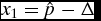 $x_1=\hat{p}-\Delta$
and
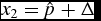 $x_2=\hat{p}+\Delta$
, for
 $\Delta \le \hat{p}$
, where x
1 is on the left bridge and x
2 on the right-side bridge. The above expressions then become
 $$\begin{eqnarray*}
\frac{d}{dp} \left(\sigma _{x_1}^{p} \right) &=&-\sigma \frac{x_1}{2}\sqrt{\frac{1}{p\left(1-p\right)}}.\frac{1}{p}, \quad\text{and,}\\
\frac{d}{dp} \left(\sigma _{x_2}^{p} \right) &=&\sigma \frac{1-x_2}{2}\sqrt{\frac{1}{p\left(1-p\right)}}.\frac{1}{\left(1-p\right)}
\end{eqnarray*}$$
Taking the ratio
 $$\begin{eqnarray}
\frac{-\frac{d}{dp} \left(\sigma _{x_1}^{p} \right)}{\frac{d}{dp} \left(\sigma _{x_2}^{p} \right)} =\frac{x_1}{1-x_2}.\frac{1-p}{p} =\frac{\hat{p}-\Delta }{1-\hat{p}-\Delta }.\frac{1-p}{p},
\end{eqnarray}$$
at
 $p=\hat{p}$
, we have
 $$\begin{eqnarray}
\frac{-\frac{d}{dp} \left(\sigma _{x_1}^{p} \right)}{\frac{d}{dp} \left(\sigma _{x_2}^{p} \right)} &=&\frac{\hat{p}-\Delta }{1-\hat{p}-\Delta }.\frac{1-\hat{p}}{\hat{p}}=\frac{\hat{p}-\Delta }{\hat{p}}.\frac{1}{\frac{1-\hat{p}-\Delta }{1-\hat{p}}}\nonumber\\
&=&\frac{1-\frac{\Delta }{\hat{p}}}{1-\frac{\Delta }{1-\hat{p}}} \le 1 \text{ if } \hat{p}\le \frac{1}{2},
\end{eqnarray}$$
with the inequality strict if
 $\hat{p}< \frac{1}{2}$
. This implies that the marginal decrease in standard deviation at x
1 is dominated by the marginal increase in standard deviation at x
2. At
 $\hat{p}=p^*<\frac{1}{2}$
, the distributions at x
1 and x
2 have means that are equally distant from zero but with differing standard deviations, specifically σ
p
x
2
> σ
p
x
1
as
 $p^* <\frac{1}{2}$
.
Differentiating Equation (8),
 $$\begin{eqnarray}
\frac{d^2V_q^p}{d\left(\sigma _{q}^{p}\right)^2} = \frac{2e^{-\frac{\left(\mu _q\right)^2}{2\left(\sigma _{q}^{p}\right)^2}}}{\sqrt{2\pi }} \frac{\left(\mu _q\right)^2}{\left(\sigma _{q}^{p}\right)^3}>0.
\end{eqnarray}$$
This says that a unit increase in standard deviation is more valuable at x
2 than at x
1. Combined with Equation (10), we have that at p*, an increase in p increases utility at x
2 by more than it decreases utility at x
1. Aggregating across all matched pairs, we conclude that expected utility is increasing in p for the set of case facts (0, 2p*). The remaining case facts, (2p*, 1), are on the right-side bridge. For these cases the reduction in variance from hearing p is increasing in p, which by the argument above and Equation (8) implies expected utility is increasing in p. Thus, at p = p* outcome expected utility is strictly increasing in p and p* cannot be the optimal case to hear. The reverse logic holds when
 $p^*>\frac{1}{2}$
.
Parts (i) and (ii) of the proposition are perfectly analogous, so without loss of generality consider Part (i), the situation analyzed above, and suppose
 $\hat{p}<p^*$
. The inequality in Equation (10) continues to hold and is strict. The comparison of x
1 and x
2 now involves different standard deviations and expected values that are not equally distant from the zero threshold; specifically, μ
x
1
> |μ
x
2
|. Differentiating Equation (8) with respect to μ
q
, however, gives
 $$\begin{eqnarray}
\frac{d^2V_q^p}{d\sigma _{q}^{p}d\mu _{q}} = \frac{2e^{-\frac{\left(\mu _q\right)^2}{2\left(\sigma _{q}^{p}\right)^2}}}{\sqrt{2\pi }} \frac{-\mu _q}{\left(\sigma _{q}^{p}\right)^2} < 0.
\end{eqnarray}$$
This, combined with Equation (11), implies that the marginal value of an increase in standard deviation is greater at x
2 than at x
1. Thus, the logic of the previous proof at p = p* generalizes to all
 $\hat{p}<p^*$
. A rearrangement of terms shows that a similar dominance relationship exists for all
 $\hat{p}>\frac{1}{2}$
, and, therefore, the optimal p must lie in the interval
 $\left(p^*,\frac{1}{2}\right)$
, as required.
Part (iii). Requires b = −1, which implies that
 $p^*=\frac{1}{2}$
. At t = |b| = 1, the ratio in Equation (9) is exactly one and the matched points x
1 and x
2 have equal standard deviation and collectively span the entirety of the bridge [0, 1]. This implies that marginal expected utility is zero at p = p* as required.
Proof of Proposition 2: The result follows from an analogous pairwise matching of case facts as in the proof of Proposition 1, noting that the expected outcome of case facts closer to the lower end of the bridge are closer to zero than at the higher end.
Proof of Proposition 3: The result follows from an analogous pairwise matching of case facts as in the proof of Proposition 1, noting that for pairs of case facts with outcomes on either side of zero, the variance is higher for for case facts on the opposite side of zero to the on point precedent.
Proof of Proposition 4: The path of
 $\mathbb {E}\left[\psi\,\; \left( p\right) \right]$
is continuous, from Properties 1 and 2. Consider an interval of standard exploitative cases. Linearity of the bridge implies the cut point of zero is unique. Hearing a case on the bridge splits the bridge into two. Linearity and continuity implies that, for both bridges combined, a unique crossing exists and doctrinal complexity is unchanged. For the doctrinal cut point to remain unchanged, we require
 $\psi\,\; \left( p\right)=\mathbb {E}\left[\psi\,\; \left( p\right) \right]$
, a zero probability event. For nonstandard cases the initial bridge does not cross zero. Thus doctrinal complexity cannot decrease and a realization as in Figure 3 demonstrates the possibility of an increase. An increase occurs only for outcomes on one side of the expected outcome, and thus occurs with less than
 $\frac{1}{2}$
probability.
These arguments also hold for exploratory cases by applying the fact that
 $\mathbb {E}\left[\psi\,\; \left( p\right) \right] \rightarrow \pm \infty$
as p → ±∞.
Proof of Proposition 5: Suppose the Higher Court hears exploratory cases until a bridge is formed that crosses zero (i.e., until a standard exploitative case exists); by Proposition 3 this happens with probability greater than
 $\frac{1}{2}$
each period and, therefore, with probability one in finite time. Consider now experimenting on the bridge. It is straightforward to show that the expected utility from a bridge is linear in the width of the bridge. As the width of the bridge approaches zero, therefore, expected utility approaches zero and the variance of any case facts on the bridge also approach zero. It follows that the value of hearing new cases on the bridge approaches zero as more cases are heard, and, for fixed cost of hearing cases, the Higher Court eventually stops in finite time. The same logic applies to any bridge that does not span zero (and contain nonstandard cases). The Court can then return to hearing cases on the flanks and the process just described iterates. By construction, the right-most precedent has
 $\psi\,\; \left(\bar{p}_r\right)<0$
and for hearing cases to be worthwhile,
 $p-\bar{p}_r$
is bounded away from zero. With probability 1, therefore, a ψ(p) is eventually realized that is sufficiently distant from zero to make hearing further cases unprofitable. The same logic applies to cases p <
p
l
and with probability one the Court stops hearing new cases in finite time. Finally, note that this argument does not require the clean separation of stages (the Court can switch between exploratory and exploitative cases and the logic still applies).
Proof of Proposition 6: From Equation (8) in the proof of Proposition 1 we have that
 $\frac{dV_q^p}{d\sigma }>0$
. This says that marginal utility at case facts q is strictly positive when case facts p is heard by the Higher Court, for all q for which p becomes an on point precedent. As this holds for arbitrary q, marginal expected utility is increasing in σ and the result follows.
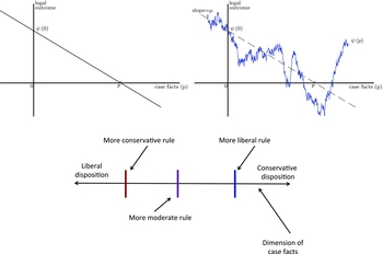
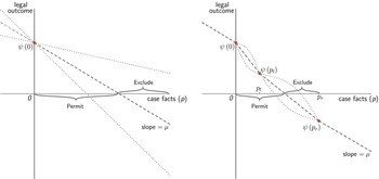
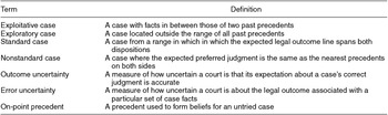
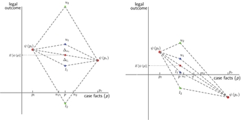
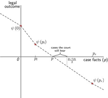
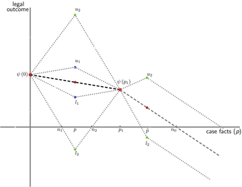



Comments
No Comments have been published for this article.