

This research note develops a new measure of trade competition, structural equivalence, and tests it in the context of the trade–environment debate.Footnote 1 This measure captures competition among countries that export similar products to the same overseas markets. We outline a new way to think about trade competition because much of the trade–environment literature tends to incorrectly equate trade competition with trade salience, the trade to gross domestic product (GDP) ratio. Not surprisingly, the empirical findings of previous research tend to be inconsistent: some studies find higher levels of trade salience to be associated with lower pollution levels,Footnote 2 while others find just the opposite.Footnote 3
The trade–environment debate is a part of a broader literature on whether international trade abets regulatory races.Footnote 4 The regulatory race hypothesis suggests that because governments tend to view themselves in situations of strategic interdependence with other countries, governments are motivated to respond to regulatory policies of competing countries.Footnote 5 The trade salience (trade/GDP), however, does not capture this sort of strategic interdependence because it is not a relational measure. While it gives us a sense of the dependence of a country on trade, it does not necessarily tell us about competitive threats from specific countries. Consider a country with a high trade salience, which is also a monopoly exporter of a scarce commodity. This country does not face strategic interdependence in its export markets because it has no competitor country whose firms can make inroads into its market share. Consequently, it does not have the incentives to change its regulatory policies in response to changes in policies of other countries. To uncover the mechanisms of regulatory races, we need to identify the competitor countries and their regulatory policies. Only with this information can we examine how trade competition might encourage strategic behavior in the regulatory arena, thereby leading to regulatory races.
Typically, a country faces competitive challenges from a variety of countries whose environmental regulatory policies exhibit varying levels of stringency. As previously mentioned, trade salience does not tell us why competitive pressure from a given country might prevail, or how pressure from different countries might be aggregated. In contrast, structural equivalence, as a measure of trade competition, enables us to aggregate pressures arising from different competitors with varying levels of regulatory stringency to estimate the levels and direction of the “net competitive pressure” that a country needs to consider.
We test our measure of trade competition in the context of the trade–environment debate by examining a panel of 140 countries for the time period 1980–2003. We find that structural equivalence is significantly associated with regulatory races, while trade salience is not associated with regulatory races. This leads us to examine whether countries respond symmetrically to the varying regulatory stringencies of their structurally equivalent competitors. Are they equally prone to ratchet down and ratchet up in response to competitive pressures? After all, a positive and statistically significant coefficient of the structural equivalence variable is consistent with a race to the bottom as well as a race to the top. Konisky's work is instructive in this regard because he demonstrates that the policy response of a given jurisdiction when its competing jurisdictions have tougher laws needs to be examined separately from when competitors have more lenient laws.Footnote 6 Testing for a race to the bottom separately from a race to the top, we find that in the case of water pollution, countries respond symmetrically to downward and upward races, that is, they follow their structurally equivalent competitor countries both when they ratchet down their regulations and when they ratchet up regulations. In the case of air pollution, however, countries are only responsive to downward policy changes in competitor countries.
The usefulness of structural equivalence as a measure of trade competition extends beyond the trade–environment literature. We believe it is particularly well suited to study how trade competition drives the cross-country diffusion of rules, norms, and practices.Footnote 7 Diffusion scholars tend to observe competitive pressures either in terms of bilateral trade patterns without making any distinction among the types of goods being tradedFootnote 8 or in terms of industry-level export profiles without making a distinction in the destination of these exports.Footnote 9 Both of these measures of trade competition can mislead. In the former, two countries exporting to the same overseas market might export different products and therefore do not compete with each other. In the latter, two countries exporting similar products might target different overseas markets. Here again, they cannot be considered as competitors who are likely to respond strategically to each other's policies. A compelling measure of trade competition must therefore reflect both the bilateral and sectoral dimensions of trade. Competing actors tend to believe that they are locked into something like a zero-sum game: if I get a share of a particular overseas market for a particular product, you cannot. This serves as a powerful motivation to respond to the policies of the competitor that might put the focal country at a disadvantage. On this count, structural equivalence is a superior measure because it captures the competitive challenge from countries whose firms export the same products to the same overseas markets.
Theoretical Approach
We use structural equivalence, a concept from social network analysis, to understand positions of specific countries in the trading network. Borgatti and Everett note that “actors who are connected in the same way to the rest of the network are said to be equivalent and to occupy the same position.”Footnote 10 Two countries that are geographically distant may have little direct contact with each other in the global economy. But if the countries are connected to the rest of the world market in a similar fashion, that is, if they export the same products to the same foreign markets, they can be said to occupy a similar network position in international commerce. This is likely to induce competition between them because from the buyer's perspective, they are substitutable. Of course, it is rare to observe exact structural equivalence in large networks of binary relationships and even harder to find it in valued networks (such as trade or communication networks), where the tie is not simply an indicator of presence or absence of a certain relationship but a measurement of the strength of this relationship (such as the volume of information flow and trade flows). Following the established practice in the social network analysis, we employ the correlation of the two actors' profiles of connections to capture the degree of their structural equivalence.Footnote 11
Structurally equivalent countries have strong incentives to be more competitive than others to secure or maintain access to the same overseas market. One way to achieve an advantage, especially for developing countries that often compete on cost rather than quality, is to lower their production and regulatory costs.Footnote 12 At the national level, governments with incentives to create a “business-friendly environment” seek to reduce regulatory costs. Countries avoid enacting new laws and even laxly enforcing the existing ones with the aim to lower firms' production and regulatory costs.Footnote 13 In competitor countries, these policies and practices are likely to be watched and mimicked, thereby creating a vicious circle in which all countries have incentives to follow one another toward environmental neglect.Footnote 14 Therefore, we propose the following key hypothesis:
H1: A country's domestic pollution intensity levels are positively related to those of its structurally equivalent competitor countries because these countries engage in competitive races in environmental regulations and their enforcement.
On the other hand, one could argue that domestic pollution levels simply reflect trade salience, irrespective of the policies of trade competitors. Therefore we add an alternative hypothesis:
H2: A country's domestic pollution intensity levels are correlated with its trade salience (trade/GDP).
Data
Dependent Variable
Arguably, to test the regulatory race hypothesis one should examine how regulatory stringency in a given country responds to the regulatory changes in countries that are structurally equivalent in the trade network. This strategy poses two problems. First, one cannot find systematic longitudinal data on stringency of environmental regulations for a sufficient cross-section of countries. Second, there is often a gap between laws on the books (de jure) and laws in practice (de facto): simply put, environmental laws might be enacted but not enforced. Indeed, in the United States, there is persistent underfunding of the Environmental Protection Agency, especially the enforcement wing, rendering the organization unable to properly enforce its own regulations.Footnote 15 Even with stringent laws on the books, governments might cut enforcement budgets, reduce penalties for enforcement violations, and adopt administrative policies, all of which undermine enforcement effectiveness. In effect, governments can (and do) diminish regulatory stringency without rewriting the law. Given these limitations, we assess levels of regulatory stringency, our dependent variable, in terms of their implication for competitiveness: pollution intensity (pollution/GDP). When existing laws are stringent and enforced, pollution intensity is low, all else equal. This would translate into higher regulatory costs for domestic firms. By the same token, if laws are not stringent and/or not enforced, pollution intensity is high, all else equal.Footnote 16 This would translate into lower regulatory costs for domestic firms.
Why not use pollution per capita as the dependent variable? We believe that pollution intensity is more relevant for our theoretical story based on trade competition because it captures environmental regulatory costs for every unit of GDP. Pollution per capita does not reflect such cost pressures. In addition, per capita pollution can be unduly influenced by the population of the country. Hence, we measure competitive pressures that bear upon domestic environmental policies in terms of pollution intensities in structurally equivalent countries.
We employ two response variables, one for air pollution—sulfur dioxide (SO2)—and one for water pollution—biochemical oxygen demand (BOD). For SO2, the variable is reported in (logged) grams of SO2 per unit of gross domestic product (measured in constant 2000 dollars based on purchasing power parity).Footnote 17 For water pollution, the variable is reported in (logged) grams of BOD per unit of gross domestic product (also measured in constant 2000 dollars based on purchasing power parity).Footnote 18
For several reasons, SO2 and BOD serve as excellent proxies for the stringency of environmental regulations. SO2 and BOD are outcomes of production processes and tend to be regulated pollutants.Footnote 19 Air and water quality are important indicators of how economic actors respect or neglect the environment. Furthermore, abatement technologies are available for both SO2 and BOD. Because these technologies have nontrivial costs, their adoption and the consequent reductions in pollution levels are likely to be influenced by competitiveness concerns.
Additionally, since we are using a panel design to test the regulatory race argument, we need to focus on response variables for which data are available for a relatively long time series.Footnote 20 Indeed, longitudinal data for SO2 and BOD emissions are available for both developed and developing countries. Finally, by using SO2 and BOD variables, we are consistent with the established practice in existing literatures. Given that our work challenges an important finding in these literatures, namely the key role of overall trade salience in driving pollution intensity levels, using SO2 and BOD as response variables should enable us to engage with a variety of audiences across the social sciences.
Independent Variables
To capture competition among countries that target the same export markets with similar products, we calculate pair-wise structural equivalence based on sector-level bilateral trade data. We employ the United Nations' Standard International Trade Classification (SITC) to identify ten broad trade sectors in international commerce: (1) food and live animals directly for food; (2) beverages and tobacco; (3) crude materials, inedible, except fuels; (4) mineral fuels, lubricants, and related materials; (5) animal and vegetable oils, fats, and waxes; (6) chemical and related products; (7) manufactured goods, classified chiefly by material; (8) machinery and transport equipment; (9) miscellaneous manufactured articles; and (10) commodities and transactions not classified elsewhere.
Structural equivalence is calculated by taking the correlation between two countries' exports at both bilateral and sector levels. Therefore, a given country's “export profile” is composed of k × (n − 1) elements in which n is the total number of countries, and k is the number of trade sectors. Data for dyadic sector-level trade are from the United Nations' Comtrade online database.Footnote 21 This data set covers international commerce at the dyadic level since 1962 and for different commodities detailed to the level of five-digits SITC. Aggregating bilateral trade to the one-digit level yields the ten distinct sectors that we just described.Footnote 22 A correlation matrix of each country's exports across the ten trade sectors and to all other countries is then generated to capture this structural similarity.
The value of correlation capturing the structural equivalence between countries i and j in a given year t (struc.equiv i,j,t) is bounded between −1 and 1, with 1 representing complete structural equivalence of two countries. This means these countries have the exact same profiles of bilateral exports to other countries across ten sectors of trade. The value of −1, on the other hand, captures the situation where two countries share the most dissimilar export profiles.Footnote 23
While countries naturally compete in different export markets, only those exporting the same products to the same export market are likely to consider one another competitors. We assume, therefore, that for any country i, export-induced competitive pressures only come from countries that have a positive score of structural equivalence with i, that is, only when struc.equiv i,j,t > 0. For country i, the influence from a competing exporter j in year t in setting its environmental standards can be summarized as struc.equiv i,j,t /∑j≠instruc.equiv i,j,t. Note that we have standardized struc.equiv i,j,t by ∑j≠instruc.equiv i,j,t,Footnote 24 which is the sum of the total competitive pressure faced by country i from all its competitors.Footnote 25
If country i's decision to set its environmental standards is influenced by the decisions of its key trade competitor countries, we expect its pollution intensity indicators are associated with the weighted average levels of these pollution intensities in competitor countries. We therefore use this standardized structural equivalence score to weight the pollution intensities (SO2 and BOD) in country i's competitor countries: ∑j≠in(struc.equiv i,j,t /∑j≠instruc.equiv i,j,t) × Emission j,t is therefore the weighted average of country i's competitor countries' pollution intensities. This is calculated separately for air pollution (SO2) and water pollution (BOD).
Note that the weighted average of country i's competitor countries' environment outcome indicator can be considered as a typical spatial lag term in a spatial lag model. The difference is that the weight is defined by structural equivalence in trade instead of geographical proximity. We therefore use a simpler notation w i,j,tStruc.Equiv. for structural equivalence in trade. Further, the notation yt can be thought of as a vector containing pollution intensity levels, Emission j,t for all countries in year t. The pressure from competitor countries regarding environmental regulations, as reflected in the weighted average of country i's competitor countries' pollution intensities, can therefore be expressed as a spatial lag term: wi,tStruc.Equiv.yt.Footnote 26
In addition to trade competition, our model controls for trade salience (the sum of imports and exports as a percentage of GDP) which has been used extensively in the trade–environment research. Trade could also influence pollution intensities via pressures from importing markets. Vogel's “California Effect” suggests that bilateral trade serves as a mechanism for the diffusion of importing countries' environmental standards to exporting countries.Footnote 27 The key mechanisms are customer and supplier pressure emanating from the importing country.Footnote 28 For country i, the pressure via the California Effect to adopt specific types of environmental standards can be captured by calculating the weighted average of country i's export destination countries' pollution levels. For country i, the weight for an export destination country j is determined by the relative importance of country j to country i as an export market: the higher is the salience of a given overseas market in a country's exports, the more the country is likely to follow its environmental standards. Numerically, this relative importance for a given year t can be measured as the ratio of i's exports to j (Exports i,j,t) to i's total exports (Exports i,t) of that year.Footnote 29 Therefore, the weighted average of country i's export destination countries' emission levels can be expressed as ∑j≠in(Exports i,j,t /Exports i,t) × Emission j,t, where Emission j,t is the emission level in country i's export destination country j for year t.
Again, note that Exports i,j,t /Exports i,t can also be considered as a spatial weight in a spatial model to capture the California Effect (w i,j,tCalifornia) from country j to i in year t. This measure is not defined by geographical distance as in a typical spatial model, but by the strength of export ties in international trade networks. Therefore, the whole term of bilateral exports weighted emission levels can be expressed as a spatial lag term (wi,tCaliforniayt).Footnote 30
Inward foreign direct investment (FDI) is another important factor that might impact domestic pollution levels. We measure a host country's overall dependence on inward FDI (fdi stock) based on the argument that, irrespective of the FDI's source, higher levels of inward FDI influence host countries' pollution levels. fdi stock is calculated as a host country's total inward FDI stock as a percentage of its GDP.Footnote 31
Regarding domestic drivers of environmental policy, we focus on the domestic regime type (polity). It is fair to say that the debate on the relationship between democracy and pollution levels is largely unresolved. We use the annualized Polity score, which ranges from −10 for highly authoritarian states to +10 for highly democratic societies, to gauge the effect of regime type on pollution intensity. We include both gdp per capita (in purchasing power parity) and its squared term in the baseline model to capture the curvilinear relationship between wealth and pollution levels (the Environmental Kuznets Curve).We also control for gdp growth rate. While higher growth rates often require more intensive use of resources and lead to higher levels of pollution, they may also encourage technological advancement and human capital accumulation that might eventually improve environmental quality. Thus, the directionality of the effect of growth on pollution is not clear.
Our model includes the share of industrial production in GDP because the industrial sector often exhibits higher levels of pollution intensity in relation to service and agricultural sectors. Moreover, to account for the extent to which countries rely on oil exports, our model includes a variable measuring the share of fuel exports in total exports. The conventional wisdom holds that fuel production is associated with higher levels of pollution intensity, especially for developing countries. We also include two demographic variables, population density (population/land area) and urban population (as a share of total population) to control for demographic influences on pollution levels.Footnote 32
Model and Empirical Findings
We model levels of pollution per unit of GDP in country i in year t as a function of trade competition, trade salience, California effect, inward FDI stock, and a battery of country-specific variables. The model can be written as:

where β0 is the population intercept, ϕy i,t−1 captures the effects of lagged dependent variable y i,t−1, and xi,tβ the effects of country-specific characteristics such as polity, GDP per capita, and population density.  represents the two temporarily lagged spatial lag terms of the network diffusion effects: structural equivalence in trade, that is, the weighted average of trade competitor countries' pollution intensity levels (ρs.e.wi,t−1Struc.Equiv.yt−1) and the California Effect through bilateral exports, that is, the weighted average of importing countries' pollution intensity levels (ρCaliforniawi,t−1Californiayt−1). Here,
 represents the two spatial coefficients that we estimate to capture the effects of trade competition (ρs.e.) and California Effect of trade (ρCalifornia) on environmental outcomes respectively. Notice that in order to mitigate the simultaneity bias in the estimation of spatial lag models, the spatial lags (
 ) are lagged by one year.Footnote 33 The assumption here is that outcomes in country i get influenced by outcomes in other connected countries after a time lag. Lagging the spatial lag has become a common practice in some of the recent studies of policy diffusion and neighborhood effects on policy choices,Footnote 34 mainly because it provides a simpler way to estimate the strength of interdependence (by simple ordinary least squares (OLS) regression) in relation to a spatial maximum likelihood approach (spatial ML) and spatial two-stage-least-squares instrumental variable approach (2SLS).Footnote 35 However, this strategy of lagging the spatial lag terms is based on a strong assumption, that is, the absence of instantaneous effect.Footnote 36 Moreover, in the analysis of spatial interdependence, it is of great importance that common external shocks (for example, oil crisis) are controlled and distinguished from interdependence.Footnote 37 Equation (1) therefore includes year dummy variables (T t) to control for potential common shocks. Finally, we allow for cross-sectional heterogeneity by including country fixed effects (C i).
Table 1 (Models 1, 2, and 3) and Table 2 (Models 4, 5, and 6) present the empirical findings regarding the impact of trade competition on air pollution (SO2) and water pollution (BOD). Model 1 reports a statistically significant effect of trade competition on SO2 emission intensity. However, in Model 3 in which the California Effect of trade is also included, there appears to be no significant relationship between trade competition and SO2 emission intensity (p = .14 in a two-tailed test). Moreover, we do not observe a significant effect of the California Effect of trade on SO2 emissions as illustrated in Models 2 and 3. This suggests that exporting countries' SO2 emission intensities are not affected by the emission intensities of their overseas destinations. Importantly, trade salience, the key variable that previous research has employed to test the link between trade and pollution, is not significant in any model specifications in Table 1.
Modeling SO2 emission per unit of GDP, 1981 to 2003

Notes: 1980 enters the analysis in the lagged dependent variable and spatial lags only. Country and year fixed effects are estimated for all models but not reported because of space constraints. p > |t| data are in parentheses.
Modeling BOD discharge per unit of GDP, 1981 to 2003

Notes: 1980 enters the analysis in only the lagged dependent variable and spatial lags. Country and year fixed effects are estimated for all models but not reported because of space constraints. p > |t| data are in parentheses.
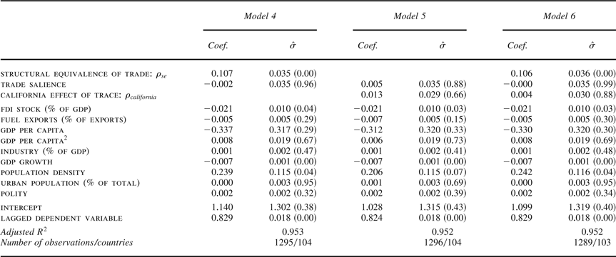
Table 2 reports our findings on the effect of trade competition on water pollution (BOD). We find similar results regarding the effects of the California Effect and trade salience: the California Effect variable does not have significant effect in any model specification, suggesting that importing countries' water pollution intensities do not influence exporting countries' pollution levels. Consistent with Table 1, we find that trade salience is not a significant driver of water pollution (Table 2).
The key difference pertains to the effect of trade competition: unlike SO2, we find a significant and positive correlation between the structural equivalence and BOD pollution intensity, with or without the inclusion of the California Effect variable. The estimated spatial coefficient is around 0.11 in both model specifications. This means that if country i's trade competitors' weighted average BOD discharge intensity increases by one unit (in log scale) in year t−1, country i's emission level is expected to increase by 0.11 unit (logged grams per unit of GDP) in the subsequent year.
What might explain the consistent support for the relationship between structural equivalence and BOD discharges, but not between structural equivalence and SO2 emissions? The largest share of SO2 emissions stems from stationary sources, mostly electricity generation and iron and steel industries. For most countries, the products emanating from such activities comprise only a small part of their overall exports. In contrast, there are several industries in a typical exporting economy that tend to contribute to water pollution. This suggests that SO2 emissions are likely to be less sensitive to pressures from trade competitors than BOD discharges.Footnote 38
Regarding the effects of domestic variables in Tables 1 and 2, only GDP growth has a consistent and significant effect on both SO2 emissions and BOD discharges. This negative effect, we suspect, might be a function of technological advancement and human capital accumulation as a result of economic growth. Other variables, on the other hand, do not have consistent correlation with SO2 and BOD. FDI stocks are associated only with lower level of BOD discharges (see Models 4 to 6 in Table 2). The inverted U-shape Kuznets Curve is evident only for SO2 emissions (see Models 1 to 3 in Table 1). Also, the salience of the industrial sector in the GDP is significantly correlated only with SO2 emissions (Table 1). Population density increases BOD discharges but not SO2 emissions. Urban population, on the other hand, has just the opposite effect: it increases SO2 emissions but not BOD discharges. More democratic countries are associated with higher levels of SO2 emissions but not correlated with BOD discharges. Finally, salience of oil exports in overall exports does not affect either air pollution (SO2) or water pollution (BOD).
We also ran our baseline models separately for Cold War and post–Cold War periods, for non–European Union (EU) countries and non–Organization for Economic Cooperation and Development (OECD) countries. The basic finding of a consistent and significant association between structural equivalence and water pollution intensity holds across all these scenarios. The statistical association between trade competition and air pollution intensity, on the other hand, is not consistently significant.
Controlling for Economic Similarity
One might wonder whether the relationship between pollution and structural equivalence is spurious because both are endogenous to domestic economic structures. After all, economies with similar sectoral concentrations should exhibit similar pollution intensity levels as well as similar export profiles. In Tables 1 and 2 (Models 1 to 6), we employed two variables to control for economic similarity: (1) the share of industrial production in GDP because industrial production often generates more pollution than service and agricultural sectors; and (2) the share of fuel exports in total exports because fuel production tends to be highly polluting. In addition, we included fixed country effects to control for cross-country heterogeneity, part of which is a function of variations in sectoral profiles of national economies.
Arguably, the above controls imperfectly account for economic similarity. Ideally, our model should include a similarity indicator for each country-pair in terms of the sectoral composition of the economy. To accomplish this, one requires longitudinal data on domestic production and pollution intensities at the sectoral level for a sizeable cross-section of countries. As far as we know, such data covering most of the countries in our study do not exist. Thus, we construct reasonable proxies for economic similarity. We propose two sets of proxies: (1) education and physical infrastructure similarities and (2) the salience of polluting exports in overall exports. For the education–infrastructure proxy, we focus on education and infrastructure characteristics of the economy. The assumption is that countries with similar education and infrastructural profiles are likely to exhibit similar domestic production profiles. For the export-based proxy, we employ the share of high pollution intensity commodity exports in total exports as a proxy for the salience of pollution intensive sectors in the domestic economy. These proxies are discussed below.
Education–Infrastructure Proxy for Economic Similarity
We consider ten indictors of national education characteristics:
1. Gross intake rate in first grade (percentage of relevant age group)
2. Labor force with primary education (percentage of total)
3. Labor force with secondary education (percentage of total)
4. Labor force with tertiary education (percentage of total)
5. Labor skills (percentage of managers surveyed ranking this as a major business constraint)
6. Literacy rate, adult total (percentage of people ages fifteen and above)
7. Net intake rate in grade 1 (percentage of official school-age population)
8. Persistence to fifth grade (percentage of cohort)
9. Primary completion rate (percentage of relevant age group)
10. Progression to secondary school (percentage)
We also consider the following thirteen indicators to characterize a country's infrastructural profile:
1. Financial information infrastructure index (0 = less developed to 10 = more developed)
2. Fixed line and mobile phone subscribers (per 1,000 people)
3. Health expenditure per capita (current U.S.$)
4. Information and communication technology expenditure per capita (U.S.$)
5. Internet users (per 1,000 people)
6. Mobile phone subscribers (per 1,000 people)
7. Personal computers (per 1,000 people)
8. Rail lines (route–kilometer per square kilometer)
9. Researchers in research and development (per million people)
10. Roads, total network (kilometer per square kilometer)
11. Telephone average cost of call to United States (U.S.$ per three minutes)
12. Telephone mainlines (per 1,000 people)
13. Vehicles (per 1,000 people)
In constructing the education-infrastructure similarity measure, we follow the logic employed in the construction of trade competition measure (structural equivalence): we take the correlation between country i's and j's education-infrastructure profiles (a total of twenty-three indicators).Footnote 39 Following the same strategy to construct the spatial lag for trade competition, we construct a spatial lag to capture the effect of economic similarity on countries' pollution intensity: ∑j≠inw i,j,tSim:Educ,Infrast × Emission j,t is the average pollution intensity of countries weighted by their similarity with country i in terms of the education-infrastructure profile.
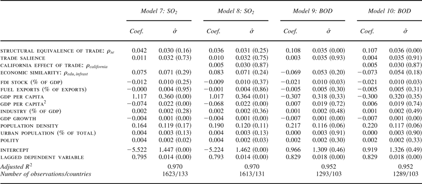
The empirical findings with the inclusion of the education-infrastructure spatial lag in the model are reported in Table 3.Footnote 40 Even after controlling for economic similarity, we find a significant relationship between structural equivalence and water pollution (BOD). Consistent with our findings in the previous section, the relationship between structural equivalence and air pollution (SO2) is not significant.Footnote 41
Trade competition and pollution intensity after controlling for economic similarity: using similarity in education and infrastructure as proxy

Notes: 1980 enters the analysis in only the lagged dependent variable and spatial lags. Country and year fixed effects are estimated for all models but not reported because of space constraints. p > |t| data are in parentheses.
Export-Based Proxy
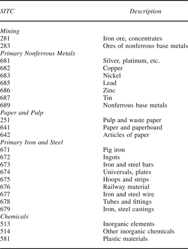
In addition to using similarity in education and infrastructure profiles as proxy for economic similarity, we consider another way to control for this potential confounding factor. We use the share of pollution intensive commodity exports in total exports as a proxy for the share of pollution intensive domestic sectors in overall domestic production. The assumption is that you export what you produce. Consistent with recent economic literature on environmental regulations and trade,Footnote 42 following Tobey, we identify the following pollution intensive commodities (Table 4).Footnote 43
Pollution intensive commodities

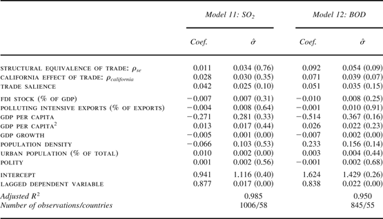
We identify commodity groups at three-digits SITC level and employ Feenstra and colleagues' trade data.Footnote 44 As a result of the limited country coverage in this data set, the number of countries included in our analysis is limited to sixty. Table 5 reports the empirical findings for both SO2 and BOD after controlling for economic similarity in terms of polluting intensive exports. Even with the inclusion of this measure of economic similarity, we observe a significant effect of trade competition on water pollution (BOD). Consistent with our previous findings, we do not find a statistically significant relationship between trade competition and air pollution (SO2).
Trade competition and pollution intensity after controlling for economic similarity: using polluting intensive exports as proxy

Notes: 1980 enters the analysis in only the lagged dependent variable and spatial lags. Country and year fixed effects are estimated but not reported because of space constraints. p > |t| data are in parentheses.
Race to the Bottom or Race to the Top?
The findings from previous sections indicate that there are strategic interactions among trade competitors regarding water pollution. However, a positive and statistically significant coefficient for structural equivalence is consistent with a race to the bottom as well as a race to the top. Would a country respond symmetrically to both higher and lower levels of environmental regulations in competitor countries? For example, if country i's trade competitors' weighted average BOD discharges are higher than its own discharges, would we expect that country i's BOD discharges to increase in the following year? Or, when country i's trade competitors' weighted average BOD discharges are lower than its own discharges, would its water pollution intensities decrease in the following year?
Following Konisky, we estimate an additional model to establish whether the “trade competition affects pollution” argument holds true separately for downward races and upward races.Footnote 45 Specifically, we estimate the following model:

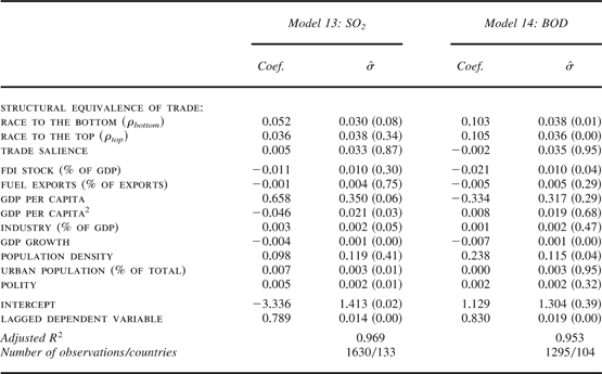
Notice that this is essentially the same model as in equation (1) except that first, we delete the spatial lag term for the California Effect because it has no significant effect on pollution intensity. Second, we split the spatial lag for trade competition, ρs.e.wi,t−1Struc.Equiv.yt−1, of equation (1) to ρbottomD i,t−1wi,t−1struct.equiv.yt−1 + ρtop(1 − D i,t−1)wi,t−1struct.equiv.yt−1, D i,t−1 = 1 when y i,t−1 < wi,t−1struct.equiv.yt−1, that is, when country i's emission intensity is lower (as a result of more stringent regulations and/or of better enforcement) than the weighted average emission intensity level of its trade competitors' in the same year t−1 (we use t−1 instead of t because the spatial lag is lagged by one year to mitigate simultaneity bias); D i,t−1 = 0 otherwise. Therefore, the spatial coefficient ρbottom is associated only with cases in which country i's emission intensity is lower than the weighted average of its trade competitor countries at the same year; that is, country i is at a cost disadvantage relative to its trade competitor countries.Footnote 46 This implies that a positive and statistically significant ρbottom supports a race to the bottom scenario. ρtop, on the other hand, indicates whether country i follows up with its trade competitors when they have lower levels of emission intensity as a result of better environmental regulations and enforcement; a positive and significant ρtop therefore provides evidence for a race to the top scenario.
We estimated models using equation (2) and report the results in Table 6 (Models 13 and 14). We find support for a race to the bottom for SO2 (Model 13) as well as for BOD (Model 14). We find evidence for a race to the top for BOD only. For SO2, the spatial coefficient (ρtop) associated with the race to top scenario lacks statistical significance (p = .34 in a two-tailed test). This might explain the statistically insignificant relationship between trade competition and SO2 in Table 1, in which strategic interactions among competitor countries are tested without making a distinction between a race to the bottom and a race to the top.
Race to the bottom or race to the top?

Notes: Country and year fixed effects not reported because of space constraints. p > |t| data are in parentheses.
Conclusion
This research note suggests that while concerns about races to the bottom in the environmental area have some empirical support, the causal story is different from the portrayal offered by globalization critics as well as some trade–environment scholars. Increasing exposure to the global market (trade salience) is not the culprit behind environmental degradation. Strategic interactions among structural equivalent trade competitor countries drive domestic pollution intensities. Therefore, a more sophisticated understanding of why countries tend to have different types of trading portfolios, how they are embedded in different types of trading networks, and how both of these might be changed is required to better understand the international and interdependent aspects of domestic environmental regulations and enforcement.
Our research note raises questions for future research. For example, some trade agreements privilege “insiders” over “outsiders” and therefore might divert trade as opposed to create trade.Footnote 47 Thus, trade agreements will influence the composition of the trade networks and therefore influence the competitive pressures member countries as well as nonmember countries face. Such less-recognized consequences of trade agreements need more analysis and scrutiny. This research note also suggests that when governments encourage specific sectors for exports—through subsidies, infrastructure investment, or foreign exchange provision—they also influence domestic environmental outcomes by changing the positions of the national economy in the global trade network, thereby subjecting themselves to different types and levels of competitive pressures. In a similar vein, multilateral funding agencies should recognize the environmental implications of their economic advice, not only in terms of purely domestic considerations, which they routinely do via environmental impact analyses, but also in terms of trade implications.
Our note brings both good and bad news to environmentalists and activist groups that are worried about the environmental consequences of global trade. The task for these groups is to manipulate the trade context in which countries operate with the objective to encourage upward races or discourage downward races. Indeed, environmental groups can harness the trading system to their advantage if they can identify the key trade competitors of a given country and then work on improving environmental laws and practices in these competitor countries. The challenge is to identify the pressure points and to subject them to political and economic pressure to improve levels of environmental protection. Narrowly focusing on an individual country is not enough because of strong externalities of environmental policies and regulations in trade competitor countries. Multilateral efforts targeting countries belonging to the same group of competitor countries might be better at dealing with environmental problems. In sum, while more research is certainly needed to better understand the intricate connections between trade and environmental regulations, we hope this note has provided a solid foundation for this new and exciting area of future research.
 . Notice that ɛi,t−1 is the error term for the right-hand-side variable y i,t−1. The fact that they are both at the right-hand side of the equation gives rise to simultaneity bias. Including a lagged dependent variable (ϕy i,t−1) often helps to mitigate serial correlation in the errors, but there is no guarantee. Therefore, using a Lagrange Multiplier test, we test the existence of serial correlation in error terms after estimating equation (