1. Introduction
Recently, nonlinear wave propagation in plasmas has become one of the most important subjects in plasma physics. The properties of these nonlinear plasma waves can be described by different nonlinear differential equations, e.g. the Korteweg–de Vries (KdV) equation, modified KdV equation and nonlinear Schrödinger equation Dodd et al. (Reference Dodd1982), in one dimension. The ion acoustic (IA) mode is a fundamental mode in a plasma. This mode has been studied in different plasma systems having different combinations of plasma species. The pseudopotential approach and the reductive perturbation method (RPM) have been employed to study these nonlinear waves in arbitrary and small amplitude limits, respectively. Washimi & Taniuti (Reference Washimi and Taniuti1966) were the first to derive the KdV equation for IA solitons in a plasma. Later, Zakharov & Kuznetsov (Reference Zakharov and Kuznetsov1974) derived a Zakharov–Kuznetsov (ZK) equation for describing nonlinear IA waves in a magnetized plasma composed of cold ions and hot isothermal electrons. The IA solitons were studied theoretically, and later were observed experimentally (Tran Reference Tran1979; Nakamura Reference Nakamura1982; Lonngren Reference Lonngren1998; Saitou & Nakamura Reference Saitou and Nakamura2005). Moreover, Samanta, Saha & Chatterjee (Reference Samanta, Saha and Chatterjee2013) described the nonlinear properties of plasma waves in more than one dimension using ZK and Kadomtsev–Petviashili (KP) equations.
The electron–positron (EP) plasmas are found in different astrophysical plasma situations such as active galactic nuclei, quasars, neutron stars and pulsar magnetospheres. (Stenflo, Shukla & Yu Reference Stenflo, Shukla and Yu1985; Miller & Wiita Reference Miller and Wiita1987; Iwamoto Reference Iwamoto1993; Zank & Greaves Reference Zank and Greaves1995; Reynolds et al. Reference Reynolds1996; Hirotani et al. Reference Hirotani1999). The EP plasma, which consists of identical mass but oppositely charged particles, has quite different dynamics than that of the usual electron–ion (EI) plasma in which both fast and slow time scales exist. The symmetry of EP plasma dynamics breaks in the presence of ions, and both fast and slow time scales occur in electron–positron–ion (EPI) plasma. In most astrophysical environments, EP plasma exists in the relativistic regime. The linear and nonlinear electrostatic and electromagnetic waves in EPI plasmas have already been studied by a number of authors (Yu, Shukla & Stenflo Reference Yu, Shukla and Stenflo1986; Popel, Vladimirov & Shukla Reference Popel, Vladimirov and Shukla1995; Mahajan, Berezhiani & Mikilaszewski Reference Mahajan, Berezhiani and Mikilaszewski1998; Mahmood, Mushtaq & Saleem Reference Mahmood, Mushtaq and Saleem2003; Mahmood & Ur-Rehman Reference Mahmood and Ur-Rehman2009; Mahmood, Akhtar & Ur-Rehman Reference Mahmood, Akhtar and Ur-Rehman2011).
The behaviours of plasma particles are significantly changed by the inclusion of magnetic field effects (Das & Verheest Reference Das and Verheest1989; El-Taibany, El-Bedwehy & El-Shamy Reference El-Taibany, El-Bedwehy and El-Shamy2011). Mace & Hellberg (Reference Mace and Hellberg2001) investigated the effect of an external magnetic field on weakly nonlinear electron acoustic waves and they derived what they termed the KdV–ZK equation for describing such waves. Later, Mahmood & Akhtar (Reference Mahmood and Akhtar2008) studied the IA solitary wave (IASW) structures in multi-component magnetized plasmas with adiabatically heated ions. They explained the variations of these solitary wave structures in the presence of an external magnetic field and applied their findings to pulsar cusp regions. The nonlinear electrostatic drift waves in dense EPI and multi-component plasmas have also been investigated by (Haque, Mahmood & Mushtaq Reference Haque, Mahmood and Mushtaq2008). Mushtaq, Saeed & Haque (Reference Mushtaq, Saeed and Haque2009) have studied IA waves in a magnetized pair EI plasma and have derived a ZK equation for pair EI plasmas. It is revealed that nonlinear profiles of the IASW are significantly affected by the obliqueness propagation angle, magnetic field and the electron concentration. Also, Kourakis et al. (Reference Kourakis2009) have derived a ZK equation to study the rotational effect on the formation of multi-dimensional solitons in EPI and pair ion plasmas.
The Maxwellian distribution is a velocity distribution describing the plasma particles in a thermal equilibrium but it is not suitable for non-thermal space and laboratory plasmas (Maksimovic, Pierrard & Riley Reference Maksimovic, Pierrard and Riley1997; Leubner Reference Leubner2004; Christon et al. Reference Christon2012). Most plasma studies have been carried out considering the system components are in thermal equilibrium, whereas the ideal thermal equilibrium assumption is no longer valid where some external agents (e.g. external force fields present in natural space plasma environments, wave-particle interactions, turbulence, etc.) disturb this equilibrium state. The deviation of the Maxwellian distribution takes place when the fluid velocity is much greater than the thermal velocity, or the plasma particles move very fast compared to their thermal velocities, particularly in space and astrophysical environments (Asbridge, Bame & Strong Reference Asbridge, Bame and Strong1968; Divine & Garret Reference Divine and Garret1983; Futaana et al. Reference Futaana2003).
Over the last few decades, a great deal of attention has been paid to a non-extensive generalization of the Boltzmann–Gibbs–Shannon (BGS) entropy, first recognized by Renyi (Reference Renyi1955) and subsequently proposed by Tsallis (Reference Tsallis1988). In some space regions, distribution functions having non-Maxwellian energy tails, or flat topped structures with pronounced shoulders, are observed. During the last two decades, it has been proven that Boltzmann–Gibbs (BG) statistics are not appropriate to describe correctly systems with long range interaction, long time memory and fractality of the corresponding space-time/phase-space etc. The main reason for this failure is due to the fact that BG statistics are extensive and additive in its formalism. In order to analyse the statistical properties of the system with long range correlations, Tsallis (Reference Tsallis1988, Reference Tsallis1995) extended BG thermodynamics by generalizing the concept of entropy to cover the non-extensive regime. Non-extensivity means that the entropy of the composition
 $(A+B)$
of two independent systems,
 $A$
and
 $B$
, is equal to
 $S_{q}(A+B)=S_{q}(A)+S_{q}(B)-(1-q)S_{q}(A)S_{q}(B)$
where the parameter
 $q$
defines the non-extensivity property and it is referred to as the entropic index of the non-extensive system under consideration. Statistically, this distribution can be viewed as a simple reparametrization of the student distribution first introduced by Gosset (Reference Gosset1908). Among the various physical systems in which connections with Tsallis entropy have been found are plasma physics (Lima, Silva & Santos Reference Lima, Silva and Santos2000; Munoz Reference Munoz2006), long-range Hamiltonian systems (Latora, Rapisarda & Tsallis Reference Latora, Rapisarda and Tsallis2001), gravitational systems (Taruya & Sakagami Reference Taruya and Sakagami2003) and many other applications (Abe & Okamoto Reference Abe and Okamoto2001). Lima et al. (Reference Lima, Silva and Santos2000) have found that the
 $q$
-non-extensive pattern is very important for systems having long-range interactions (i.e. studying interactions that are comparable to the size of the system under consideration) such as those occurring in astrophysics and plasma physics. Moreover, Liu et al. (Reference Liu1994) and Lima et al. (Reference Lima, Silva and Santos2000) have showed that the plasma experimental results lead to a non-Maxwellian velocity distribution. Very recently, the Tsallis
 $q$
-entropy and the ensuing generalized statistics have been employed with noticeable success to various plasma physics models (Jain, Tiwari & Sharma Reference Jain, Tiwari and Sharma1990; Du Reference Du2004; Verheest et al.
Reference Verheest2006; Liyan & Jiulin Reference Liyan and Jiulin2008; Tribeche, Djebarni & Amour Reference Tribeche, Djebarni and Amour2010; Bains et al.
Reference Bains, Tribeche, Saini and Gill2011; El-Taibany & Tribeche Reference El-Taibany and Tribeche2012; Ghosh, Chatterjee & Roychoudhury Reference Ghosh, Chatterjee and Roychoudhury2012; Akhtar, El-Taibany & Mahmood Reference Akhtar, El-Taibany and Mahmood2013; Hussain, Akhtar & Mahmood Reference Hussain, Akhtar and Mahmood2013; Shan & Akhtar Reference Shan and Akhtar2013). For example, Ghosh et al. (Reference Ghosh, Chatterjee and Roychoudhury2012) have investigated the head-on collisions of IASW in the presence of
 $q$
-distributed electrons. Also, the arbitrary-amplitude IASW is studied in a two component plasma with
 $q$
-non-extensive electron velocity distribution, (Tribeche et al.
Reference Tribeche, Djebarni and Amour2010). Their results show that the plasma model admits both compressive and rarefactive IA solitons whose amplitudes are sensitively dependent on the
 $q$
-non-extensive parameter. In addition, Bains et al. (Reference Bains, Tribeche, Saini and Gill2011) have discussed a magnetized plasma model, including
 $q$
-distributed electrons, by deriving a nonlinear ZK equation. The nonlinear propagation of large amplitude IA waves in a magnetized plasma, composed of kappa-distributed electrons and an inertial ion fluid, has been recently investigated by Sultana et al. (Reference Sultana2010) using the Sagdeev potential analysis. Their results prove that the presence of excess superthermal electrons and a magnetic field influences the nature of the solitary wave profile. Sagdeev potential analysis has been used to address the effect of non-extensive electrons and thermal positrons on the IASW and double layers (Sahu Reference Sahu2011). Saini & Shalini (Reference Saini2013) addressed the problem of IASW in a plasma with two temperature electrons that obey
 $q$
-non-extensive distribution. The modulation properties and stability regions of electron acoustic wave (EAW) are studied in two-dimensional plasma (Saini & Kholi Reference Saini and Kholi2014). Nsengiyumva et al. (Reference Nsengiyumva2014) have studied the existence domains of arbitrary amplitude fast mode IA solitons in a plasma composed of warm adiabatic and cold positive ion species in the presence of Boltzmann electrons. The analysis of linear electrostatic waves in four component electron positron plasmas using the fluid equations has been carried out (Lazarus et al.
Reference Lazarus2012a
). Later, Lazarus et al. (Reference Lazarus2012b
) investigated the existence of arbitrary amplitude solitons in a relativistic electron positron, unmagnetized plasmas. The IA soliton amplitude increases with the increase in superthermality of electrons as discussed (Singh et al.
Reference Singh2013).
In the present paper, employing RPM (Washimi & Taniuti Reference Washimi and Taniuti1966; Kourakis et al.
Reference Kourakis2009), we derive a ZK equation adequate for describing IASW in a warm magnetized EPI plasma including
 $q$
-non-extensive electrons and positrons and inertial ion fluid. The stability of the produced two-dimensional solitons is also addressed. The paper is organized as follows: the basic set of equations governing the dynamics of nonlinear IASW waves in a magnetized EPI plasma including non-extensive electrons and positrons is presented in § 2. Using RPM, a ZK equation is derived and the predicted soliton solutions are derived in § 3. The introduction of the instability of the produced solitons using the small
 $k$
-expansion method (Moslem et al.
Reference Moslem2007; Ghosh & Chakrabart Reference Ghosh and Chakrabart2013) is in § 3 as well. The present results are numerically illustrated and discussed in § 4. The conclusions are summarized in § 5.
2. Basic set of equations
A magnetized EPI plasma is under consideration, which is comprised of
 $q$
-distributed electrons and positrons, as well as inertial warm ions. An external magnetic field of strength
 $B_{0}$
is applied along the
 $x$
-axis i.e.
 $\boldsymbol{B}_{0}=B_{0}\hat{x}$
. The charge neutrality condition at equilibrium is
 $n_{e0}=n_{i0}+n_{p0},$
where
 $n_{j0}$
is the equilibrium number density of
 $j$
th species (
 $j=\text{e}$
for electrons,
 $\text{i}$
for ions and
 $\text{p}$
for positrons).
The nonlinear dynamics of the IA waves in the proposed magnetized plasma can be described by the following equation of ion continuity,
 $$\begin{eqnarray}\frac{\partial n_{i}}{\partial t}+\boldsymbol{{\rm\nabla}}\boldsymbol{\cdot }(n_{i}\boldsymbol{V}_{i})=0,\end{eqnarray}$$
the equation of ion momentum,
 $$\begin{eqnarray}\left(\frac{\partial }{\partial t}+\boldsymbol{V}_{i}\boldsymbol{\cdot }\boldsymbol{{\rm\nabla}}\right)\boldsymbol{V}_{i}=-\frac{e}{m_{i}}\boldsymbol{{\rm\nabla}}{\it\varphi}+{\it\omega}_{ci}(\boldsymbol{V}_{i}\times \hat{\boldsymbol{x}})-\frac{1}{n_{i}m_{i}}\boldsymbol{{\rm\nabla}}P_{i}\end{eqnarray}$$
and the Poisson equation,
 $$\begin{eqnarray}{\rm\nabla}^{2}{\it\varphi}=4{\rm\pi}e(n_{e}-n_{p}-n_{i}).\end{eqnarray}$$
The one-dimensional equilibrium
 $q$
-distribution function determining the non-extensivity behaviours of electrons and positrons (
 $j=\text{e},\text{p}$
) is given by (Silva, Plastino & Lima Reference Silva, Plastino and Lima1998; Verheest Reference Verheest2013)
 $$\begin{eqnarray}\displaystyle f(v_{j})=C_{qj}\left[1-(q_{j}-1)\left(\frac{m_{j}v_{j}^{2}}{2k_{B}T_{j}}+\frac{q_{j}{\it\varphi}}{k_{B}T_{j}}\right)\right]^{1/(q_{j}-1)}, & & \displaystyle\end{eqnarray}$$
where
 $$\begin{eqnarray}\displaystyle C_{qj}=n_{j0}\frac{{\it\Gamma}\left(\displaystyle \frac{1}{1-q_{j}}\right)}{{\it\Gamma}\left(\displaystyle \frac{1}{1-q_{j}}-\frac{1}{2}\right)}\sqrt{\frac{m_{j}(1-q_{j})}{2{\rm\pi}k_{B}T_{j}}}\quad \text{for}\;-1<q_{j}<1 & & \displaystyle\end{eqnarray}$$
and
 $$\begin{eqnarray}\displaystyle C_{qj}=n_{j0}\left(\frac{1+q_{j}}{2}\right)\frac{{\it\Gamma}\left(\displaystyle \frac{1}{q_{j}-1}+\frac{1}{2}\right)}{{\it\Gamma}\left(\displaystyle \frac{1}{q_{j}-1}\right)}\sqrt{\frac{m_{j}(q_{j}-1)}{2{\rm\pi}k_{B}T_{j}}}\quad \text{for}\;q_{j}>1. & & \displaystyle\end{eqnarray}$$
Here, the parameter
 $q_{j}$
stands for the strength of non-extensivity. It is useful to note that for
 $q_{j}<-1$
, the
 $q$
-distribution is not normalizable. In the extensive limiting case (
 $q_{j}=1$
), the
 $q$
-distribution reduces to the well-known Maxwell–Boltzmann distribution. Note that for
 $q_{j}>1$
, the
 $q$
-distribution function exhibits a thermal cutoff on the maximum value allowed for the velocity of the
 $j$
th-particles, which is given by (Pakzad & Tribeche Reference Pakzad and Tribeche2011)
 $$\begin{eqnarray}\displaystyle v_{j\,\mathit{max}}=\sqrt{\frac{2T_{j}}{m_{j}}\left(-\frac{q_{j}{\it\varphi}}{T_{j}}+\frac{1}{q_{j}-1}\right)}. & & \displaystyle\end{eqnarray}$$
The densities of
 $q$
-distributed non-thermal electrons and positrons are obtained from the zeroth order moment of the distribution function and integrating over
 $v_{j}$
i.e.
 $-\infty$
to
 $+\infty$
(for
 $q_{j}<1$
) and
 $v_{j}$
from
 $-v_{_{j}\mathit{max}}$
to
 $+v_{j\,\mathit{max}}$
(for
 $q_{j}>1$
) case, which is described as follows,
 $$\begin{eqnarray}\displaystyle & \displaystyle n_{e}=n_{e0}\left[1+(q_{e}-1)\frac{e{\it\varphi}}{T_{e}}\right]^{(q_{e}+1)/2(q_{e}-1)}, & \displaystyle\end{eqnarray}$$
 $$\begin{eqnarray}\displaystyle & \displaystyle n_{p}=n_{p0}\left[1-(q_{p}-1)\frac{e{\it\varphi}}{T_{p}}\right]^{(q_{p}+1)/2(q_{p}-1)}. & \displaystyle\end{eqnarray}$$
 $q_{e}$
and
 $q_{p}$
stand for the strengths of electron and positron non-extensivity. Unlike the description of Maxwellian distribution, such that most of the particles are centred around the thermal speed, a power law distribution characterizes the systems containing an ample supply of superthermal particles with the constraint
 $q_{e}$
,
 $q_{p}<1$
, or by including a large number of low velocity particles with the restriction
 $q_{e}$
and
 $q_{p}>1$
(Liyan & Jiulin Reference Liyan and Jiulin2008; El-Taibany & Tribeche Reference El-Taibany and Tribeche2012).
The energy of the
 $q$
-distributed particles can be obtained from the second moment of the distribution function i.e. involving the integral of
 $v_{j}^{2}f(v_{j})$
over
 $v_{j}$
, which comes out to be
 $$\begin{eqnarray}\displaystyle E_{j}=\frac{1}{2}\int v_{j}^{2}f(v_{j})\,\text{d}v_{j}=\frac{1}{(3q_{j}-1)}k_{B}T_{j} & & \displaystyle\end{eqnarray}$$
for both
 $-1<q_{j}<1$
and
 $q_{j}>1$
cases. The range of the non-extensive parameter
 $q_{j}$
(for the case
 $q_{j}<1$
) for which the energy of the system is positive should be
 $1/3<q_{j}<1$
. This is in contrast to kappa distribution theory, where the argument that the energy should remain finite has led to the standard requirement that
 ${\it\kappa}>3/2$
(Vasyliunas Reference Vasyliunas1968; Hellberg et al.
Reference Hellberg2009). There is no maximum limit for
 $q_{j}>1$
case, but its values are not taken to be very large in the literature (Silva et al.
Reference Silva, Plastino and Lima1998; Pakzad & Tribeche Reference Pakzad and Tribeche2011; Verheest Reference Verheest2013) for a non-thermal plasma system.
Here
 $\boldsymbol{{\rm\nabla}}=(\partial /\partial x,\partial /\partial y,0)$
and
 $\boldsymbol{V}_{i}=(V_{ix},V_{iy},V_{iz})$
and the quantities
 $n_{j}$
and
 ${\it\varphi}$
are the number density of
 $j$
th species and the electrostatic potential, respectively. The ion gyro-frequency is denoted by
 ${\it\omega}_{ci}=eB_{0}/m_{i}c$
,
 $e$
is the electronic charge,
 $m_{i}$
is the mass of ions and
 $c$
is the speed of light in a vacuum. For the warm ion pressure we have
 $P_{i}={\it\gamma}n_{i}T_{i}$
(Tiwari, Jain & Chawla Reference Tiwari, Jain and Chawla2007), where
 ${\it\gamma}$
is the adiabatic constant and for a magnetized plasma we have
 ${\it\gamma}=5/3$
and
 $T_{e}(T_{p})$
is the electron (positron) temperature.
Using the already mentioned dimensional equations (2.1)–(2.9), the dispersion relation in normalized form is obtained as follows
 $$\begin{eqnarray}{\it\omega}^{4}-E{\it\omega}^{2}+F=0,\end{eqnarray}$$
where
 $$\begin{eqnarray}\displaystyle & & \displaystyle E={\it\Omega}^{2}+{\it\sigma}k^{2}+\frac{k^{2}}{\displaystyle \left[k^{2}+\frac{{\it\beta}p\left(1+q_{p}\right)}{2}+\frac{{\it\mu}_{e}\left(1+q_{e}\right)}{2}\right]},\nonumber\\ \displaystyle & & \displaystyle \quad F=\left[{\it\sigma}+\frac{1}{\displaystyle \left[k^{2}+\frac{{\it\beta}p\left(1+q_{p}\right)}{2}+\frac{{\it\mu}_{e}\left(1+q_{e}\right)}{2}\right]}\right]{\it\Omega}^{2}k_{x}^{2}.\end{eqnarray}$$
Here
 $k_{x}$
and
 $k_{y}$
are the wave vectors in the
 $x$
- and
 $y$
-directions joined by the relation
 $k^{2}=k_{x}^{2}+k_{y}^{2}$
. Also,
 ${\it\lambda}_{D}=\sqrt{T_{e}/4{\rm\pi}n_{i0}e^{2}}$
(Debye length),
 ${\it\omega}_{pi}=\sqrt{4{\rm\pi}n_{i0}e^{2}/m_{i}}$
(ion plasma frequency),
 $C_{s}={\it\omega}_{pi}{\it\lambda}_{D}=\sqrt{T_{e}/m_{i}}$
(IA speed) and
 ${\it\Omega}={\it\omega}_{ci}/{\it\omega}_{pi}$
,
 ${\it\sigma}={\it\gamma}T_{i}/T_{e}$
,
 ${\it\beta}=T_{e}/T_{p}$
,
 ${\it\mu}_{e}=n_{e0}/n_{i0}$
and
 $p=n_{p0}/n_{i0}$
. The roots of the quartic equation are given by
 $$\begin{eqnarray}{\it\omega}_{\pm }^{2}=\frac{E\pm \sqrt{E^{2}-4F}}{2}.\end{eqnarray}$$
The limiting cases for obliquely propagating electrostatic waves in the parallel and perpendicular directions to the magnetic field
 $\boldsymbol{B}_{0}$
are discussed below.
In order to study wave propagation in a direction parallel to the magnetic field
 $\boldsymbol{B}_{0}$
, we put
 $k_{y}=0$
in (2.13) to obtain the following two roots:
 $$\begin{eqnarray}{\it\omega}_{+}^{2}={\it\Omega}^{2},\quad {\it\omega}_{-}^{2}=\frac{\left[{\it\sigma}k_{x}^{2}+{\it\sigma}\left(\displaystyle \frac{{\it\beta}p(1+q_{p})}{2}+\displaystyle \frac{{\it\mu}_{e}(1+q_{e})}{2}\right)+1\right]}{\left(k_{x}^{2}+\displaystyle \frac{{\it\beta}p(1+q_{p})}{2}+\displaystyle \frac{{\it\mu}_{e}(1+q_{e})}{2}\right)}k_{x}^{2}.\end{eqnarray}$$
The positive root is a frequency and can therefore be neglected; the second root is the dispersion relation for an IA wave propagating along the magnetic field and the phase velocity of IA wave depends on the non-extensive parameters of the electrons and positrons, temperature and their density ratios.
On the other side, to find the electrostatic wave propagating in a direction perpendicular to the magnetic field
 $\boldsymbol{B}_{0}$
, we put
 $k_{x}=0$
in (2.13) and obtain
 $$\begin{eqnarray}{\it\omega}_{+}^{2}={\it\Omega}^{2}+\frac{\left[{\it\sigma}k_{y}^{2}+{\it\sigma}\left(\displaystyle \frac{{\it\beta}p(1+q_{p})}{2}+\displaystyle \frac{{\it\mu}_{e}(1+q_{e})}{2}\right)+1\right]}{\left(k_{y}^{2}+\displaystyle \frac{{\it\beta}p(1+q_{p})}{2}+\displaystyle \frac{{\it\mu}_{e}(1+q_{e})}{2}\right)}k_{y}^{2},\quad {\it\omega}_{-}^{2}=0.\end{eqnarray}$$
The positive root gives the dispersion relation for an ion cyclotron wave (ICW), whereas the slow wave vanishes. Here, the phase velocity of the ICW is not independent of
 $k_{y}$
and also depends on the non-extensive parameters of the electrons and positrons, temperature and their density ratios.
We can express (2.1)–(2.9) in the form of scalar components as follows,
 $$\begin{eqnarray}\displaystyle & \displaystyle \frac{\partial n_{i}}{\partial t}+\frac{\partial }{\partial x}n_{i}V_{ix}+\frac{\partial }{\partial y}n_{i}V_{iy}=0, & \displaystyle\end{eqnarray}$$
 $$\begin{eqnarray}\displaystyle & \displaystyle \left(\frac{\partial }{\partial t}+V_{ix}\frac{\partial }{\partial x}+V_{iy}\frac{\partial }{\partial y}\right)V_{ix}=-\frac{\partial {\it\Phi}}{\partial x}-\frac{{\it\sigma}}{n_{i}}\frac{\partial n_{i}}{\partial x}, & \displaystyle\end{eqnarray}$$
 $$\begin{eqnarray}\displaystyle & \displaystyle \left(\frac{\partial }{\partial t}+V_{ix}\frac{\partial }{\partial x}+V_{iy}\frac{\partial }{\partial y}\right)V_{iy}=-\frac{\partial {\it\Phi}}{\partial y}+{\it\Omega}V_{iz}-\frac{{\it\sigma}}{n_{i}}\frac{\partial n_{i}}{\partial y}, & \displaystyle\end{eqnarray}$$
 $$\begin{eqnarray}\displaystyle & \displaystyle \left(\frac{\partial }{\partial t}+V_{ix}\frac{\partial }{\partial x}+V_{iy}\frac{\partial }{\partial y}\right)V_{iz}=-{\it\Omega}V_{iy}, & \displaystyle\end{eqnarray}$$
 $$\begin{eqnarray}\displaystyle & \displaystyle \left(\frac{\partial ^{2}}{\partial x^{2}}+\frac{\partial ^{2}}{\partial y^{2}}\right){\it\Phi}={\it\mu}_{e}n_{e}-n_{i}-({\it\mu}_{e}-1)n_{p}. & \displaystyle\end{eqnarray}$$
 $$\begin{eqnarray}\displaystyle & \displaystyle n_{e}=1+c_{1}{\it\Phi}-c_{1}c_{2}{\it\Phi}^{2}+\cdots \,, & \displaystyle\end{eqnarray}$$
 $$\begin{eqnarray}\displaystyle & \displaystyle n_{p}=1-p_{1}{\it\Phi}-p_{1}p_{2}{\it\Phi}^{2}+\cdots \,, & \displaystyle\end{eqnarray}$$
 $n_{e,i,p}=n_{e,i,p}/n_{e0,i0,p0},$
 $\boldsymbol{V}_{i}=\boldsymbol{V}_{i}/C_{s}$
,
 $\boldsymbol{{\rm\nabla}}=\hat{\boldsymbol{x}}\partial /\partial x+\hat{\boldsymbol{y}}\partial /\partial y\equiv \boldsymbol{{\rm\nabla}}{\it\lambda}_{D}$
,
 $t=t{\it\omega}_{pi}$
,
 ${\it\Omega}={\it\omega}_{ci}/{\it\omega}_{pi},$
and
 ${\it\Phi}=e{\it\varphi}/T_{e}.$
Here
 ${\it\mu}_{e}=(1+p),$
with,
 $c_{1}=(q_{e}+1)/2$
,
 $c_{2}=(q_{e}-3)/4$
,
 $p_{1}=(q_{p}+1){\it\beta}/2$
,
 $p_{2}=(q_{p}-3){\it\beta}/4$
. The non-extensive effects due to the electrons and positrons are represented by the indices
 $q_{e}$
and
 $q_{p}$
respectively.
3. Nonlinear analysis
In order to derive a ZK equation for the proposed magnetized EPI plasmas, we define the stretching of independent variables, from (Washimi & Taniuti Reference Washimi and Taniuti1966; Kourakis et al. Reference Kourakis2009)
 $$\begin{eqnarray}{\it\xi}={\it\epsilon}^{1/2}(x-{\it\lambda}t),\quad {\it\eta}={\it\epsilon}^{1/2}y,\quad {\it\tau}={\it\epsilon}^{3/2}t,\end{eqnarray}$$
where
 ${\it\epsilon}$
is a small
 $(0<{\it\epsilon}\leqslant 1)$
expansion parameter characterizing the strength of the nonlinearity and
 ${\it\lambda}$
(normalized by
 $C_{s}$
) is the phase speed of the wave, which will be determined later. Using the RPM, Kourakis et al. (Reference Kourakis2009), we can expand the perturbed quantities about their equilibrium values as follows:
 $$\begin{eqnarray}\displaystyle \left.\begin{array}{@{}c@{}}\displaystyle n_{j}=1+{\it\epsilon}n_{j1}+{\it\epsilon}^{2}n_{j2}+\cdots \,,\\ \displaystyle V_{ix}={\it\epsilon}V_{ix1}+{\it\epsilon}^{2}V_{ix2}+{\it\epsilon}^{3}V_{ix3}+\cdots \,,\\ \displaystyle V_{iy}={\it\epsilon}^{2}V_{iy1}+{\it\epsilon}^{3}V_{iy2}+{\it\epsilon}^{4}V_{iy3}+\cdots \,,\\ \displaystyle V_{iz}={\it\epsilon}^{3/2}V_{_{iz1}}+{\it\epsilon}^{5/2}V_{iz2}+{\it\epsilon}^{7/2}V_{iz3}+\cdots \,,\\ \displaystyle {\it\Phi}={\it\epsilon}{\it\Phi}_{1}+{\it\epsilon}^{2}{\it\Phi}_{2}+{\it\epsilon}^{3}{\it\Phi}_{3}+\cdots \,.\end{array}\!\!\right\} & & \displaystyle\end{eqnarray}$$
Substituting (3.1) and (3.2) into (2.16)–(2.22) and collecting terms of lowest order
 $({\sim}{\it\epsilon}^{3/2})$
terms of continuity and
 $x$
-,
 $y$
-,
 $z$
-components of the momentum equation for the ions, we obtain
 $$\begin{eqnarray}\displaystyle n_{i1}=\frac{{\it\Phi}_{1}}{N{\it\lambda}^{2}},\quad V_{ix1}=\frac{{\it\Phi}_{1}}{N{\it\lambda}} & & \displaystyle\end{eqnarray}$$
 $$\begin{eqnarray}\displaystyle V_{iy1}=\frac{1}{{\it\Omega}^{2}N}\frac{\partial ^{2}{\it\Phi}_{1}}{\partial {\it\xi}{\it\eta}},\quad V_{iz1}=\frac{1}{{\it\Omega}N}\frac{\partial {\it\Phi}_{1}}{\partial {\it\eta}} & & \displaystyle\end{eqnarray}$$
where
 $N=1-({\it\sigma}/{\it\lambda}^{2})$
.
The lowest order
 $({\sim}{\it\epsilon})$
terms for the non-extensive electrons and positrons from (2.21)–(2.22) give
 $$\begin{eqnarray}n_{e1}=c_{1}{\it\Phi}_{1},\quad n_{p1}=-p_{1}{\it\Phi}_{1}.\end{eqnarray}$$
The Poisson equation gives the lowest order
 $({\sim}{\it\epsilon})$
terms,
 $$\begin{eqnarray}0={\it\mu}_{e}n_{e1}-n_{i1}+(1-{\it\mu}_{e})n_{p1}.\end{eqnarray}$$
The phase speed
 ${\it\lambda}$
of the wave is obtained using (3.3), (3.5) and (3.6), i.e.
 $$\begin{eqnarray}{\it\lambda}=(N[{\it\mu}_{e}c_{1}-(1-{\it\mu}_{e})p_{1}])^{-1/2},\end{eqnarray}$$
which is the normalized phase velocity of the IA wave which can be obtained from (2.14) for a dispersionless medium.
Proceeding through the perturbation theory and using the relations provided in (3.3)–(3.7), we can finally obtain the ZK equation for an electrostatic wave in magnetized EPI plasmas in terms of
 ${\it\Phi}_{1}$
as follows,
 $$\begin{eqnarray}\frac{\partial {\it\Phi}_{1}}{\partial {\it\tau}}+A{\it\Phi}_{1}\frac{\partial {\it\Phi}_{1}}{\partial {\it\xi}}+B\frac{\partial ^{3}{\it\Phi}_{1}}{\partial {\it\xi}^{3}}+C\frac{\partial ^{3}{\it\Phi}_{1}}{\partial {\it\xi}\partial {\it\eta}^{2}}=0,\end{eqnarray}$$
where the nonlinear coefficient
 $A$
and the dispersive coefficients
 $B$
and
 $C$
are defined as,
 $$\begin{eqnarray}\displaystyle A=\frac{1}{2}\left(\frac{3}{N{\it\lambda}}-\frac{{\it\sigma}}{N{\it\lambda}^{3}}+2N^{2}{\it\lambda}^{3}[{\it\mu}_{e}c_{1}c_{2}+(1-{\it\mu}_{e})p_{1}p_{2}]\right), & & \displaystyle\end{eqnarray}$$
 $$\begin{eqnarray}\displaystyle B=\frac{N^{2}{\it\lambda}^{3}}{2},\quad \text{and}\quad C=\frac{N^{2}{\it\lambda}^{3}}{2}\left(1+\frac{1}{{\it\Omega}^{2}N^{2}{\it\lambda}}\right)\frac{\partial {\it\Phi}_{1}}{\partial {\it\eta}}. & & \displaystyle\end{eqnarray}$$
The ZK equation (3.8) has a well-known soliton solution (Kourakis et al. Reference Kourakis2009), which is given by
 $$\begin{eqnarray}{\it\Phi}_{1}={\it\phi}_{m}\text{sech}^{2}({\it\zeta}/W),\end{eqnarray}$$
where
 ${\it\phi}_{m}=3u_{0}/A$
and
 $W=\sqrt{4(B+C)/u_{0}}$
are the amplitude and the width of the soliton, and
 ${\it\eta}$
is the transformed coordinate in the co-moving frame with speed
 $u_{0}$
i.e.
 ${\it\zeta}=\ell _{x}{\it\xi}+\ell _{y}{\it\eta}-u_{0}{\it\tau}$
. Here
 $l_{x}^{2}+l_{y}^{2}=1$
. The coefficients of the ZK equation, which depend on the entropic indices i.e.
 $q_{e}$
and
 $q_{p}$
, directly affect the basic features of the produced soliton.
From (3.10) and the relation
 $\boldsymbol{E}_{1}=-\boldsymbol{{\rm\nabla}}{\it\Phi}_{1}$
, the normalized electric field of the obliquely propagating two-dimensional IAW becomes
 $$\begin{eqnarray}E_{1}=\frac{3u_{0}^{2/3}}{A\sqrt{(B+C)}}\tanh ({\it\zeta}/W)\text{sech}^{2}({\it\zeta}/W).\end{eqnarray}$$
Stability analysis. To study the stability of the two-dimensional solitons satisfying (3.8), we apply a small-
 $k$
expansion perturbation method (Moslem et al.
Reference Moslem2007; Ghosh & Chakrabart Reference Ghosh and Chakrabart2013). Using the following transformations
 $$\begin{eqnarray}\displaystyle X=\sqrt{\frac{A}{B}}{\it\xi},\quad T=\sqrt{\frac{A^{3}}{B}}{\it\tau},\quad Y=\sqrt{\frac{A}{C}}{\it\eta}\quad \text{and}\quad {\it\Phi}_{1}\equiv {\it\Psi}, & & \displaystyle\end{eqnarray}$$
we can rewrite (3.8) as
 $$\begin{eqnarray}\frac{\partial {\it\Psi}}{\partial T}+{\it\Psi}\frac{\partial {\it\Psi}}{\partial X}+\frac{\partial ^{3}{\it\Psi}}{\partial X^{3}}+\frac{\partial ^{3}{\it\Psi}}{\partial X\partial Y^{2}}=0.\end{eqnarray}$$
Supposing
 ${\it\chi}=X-{\it\nu}_{0}T,$
(3.13) becomes
 $$\begin{eqnarray}-{\it\nu}_{0}\frac{\partial {\it\varphi}_{0}}{\partial {\it\chi}}+{\it\varphi}_{0}\frac{\partial {\it\varphi}_{0}}{\partial {\it\chi}}+\frac{\partial ^{3}{\it\varphi}_{0}}{\partial {\it\chi}^{3}}=0,\end{eqnarray}$$
where we assume that (3.13) has a planar solution
 ${\it\varphi}_{0}$
, that is given by
 $$\begin{eqnarray}{\it\varphi}_{0}({\it\chi})={\it\varphi}_{0m}\text{sech}^{2}({\it\chi}/{\it\Delta}),\end{eqnarray}$$
with
 ${\it\varphi}_{0m}=3{\it\nu}_{0}$
and
 ${\it\Delta}=2/\sqrt{{\it\nu}_{0}}$
. Now, let us write the full solution of (3.13) as
 $$\begin{eqnarray}{\it\Psi}({\it\chi},Y,T)={\it\varphi}_{0}({\it\chi})+{\it\psi}({\it\chi})\exp (\text{i}kY-\text{i}{\it\Upsilon}T).\end{eqnarray}$$
Substituting (3.16) into (3.13) and linearizing with respect to
 ${\it\psi}$
, we obtain
 $$\begin{eqnarray}\frac{\text{d}^{3}{\it\psi}}{\text{d}{\it\chi}^{3}}+\frac{\text{d}({\it\varphi}_{0}{\it\psi})}{\text{d}{\it\chi}}-({\it\nu}_{0}+k^{2})\frac{\text{d}{\it\psi}}{\text{d}{\it\chi}}=\text{i}{\it\Upsilon}{\it\psi}.\end{eqnarray}$$
Now expanding
 ${\it\psi}$
and
 ${\it\Upsilon}$
as a power series of
 $k$
 $$\begin{eqnarray}\displaystyle \left.\begin{array}{@{}c@{}}\displaystyle {\it\psi}={\it\psi}_{0}+k{\it\psi}_{1}+k^{2}{\it\psi}_{2}+\cdots \\ \displaystyle {\it\Upsilon}=k{\it\Upsilon}_{1}+k^{2}{\it\Upsilon}_{2}+\cdots \,,\end{array}\!\!\right\} & & \displaystyle\end{eqnarray}$$
then substituting into (3.17) and equating the coefficients of equal powers of
 $k$
, the zeroth order yields
 $$\begin{eqnarray}\frac{\text{d}^{3}{\it\psi}_{0}}{\text{d}{\it\chi}^{3}}+\frac{\text{d}({\it\varphi}_{0}{\it\psi}_{0})}{\text{d}{\it\chi}}-{\it\nu}_{0}\frac{\text{d}{\it\psi}_{0}}{\text{d}{\it\chi}}=0,\end{eqnarray}$$
which can be written as
 $$\begin{eqnarray}\frac{\text{d}}{\text{d}{\it\chi}}\hat{L}({\it\psi}_{0})=0,\end{eqnarray}$$
where
 $\hat{L}=((\text{d}^{2}/\text{d}{\it\chi}^{2})+{\it\varphi}_{0}-{\it\nu}_{0})$
. Though, (3.14) can be given in terms of the operator
 $\hat{L}$
as
 $$\begin{eqnarray}\displaystyle \hat{L}\left(\frac{\text{d}{\it\varphi}_{0}}{\text{d}{\it\chi}}\right)=0. & & \displaystyle\end{eqnarray}$$
Differentiating with respect to
 ${\it\chi}$
, we obtain
 $$\begin{eqnarray}\frac{\text{d}}{\text{d}{\it\chi}}\hat{L}\left(\frac{\text{d}{\it\varphi}_{0}}{\text{d}{\it\chi}}\right)=0.\end{eqnarray}$$
Comparing (3.20) and (3.22), we can write
 $$\begin{eqnarray}{\it\psi}_{0}=\frac{\text{d}{\it\varphi}_{0}}{\text{d}{\it\chi}}.\end{eqnarray}$$
So,
 $$\begin{eqnarray}{\it\psi}_{0}({\it\chi})={\it\psi}_{0m}\text{sech}^{2}({\it\chi}/{\it\Delta})\tanh ({\it\chi}/{\it\Delta}),\end{eqnarray}$$
where
 ${\it\psi}_{0m}=-3{\it\nu}_{0}^{3/2}$
. Considering the next order of
 $k$
, one obtains
 $$\begin{eqnarray}\frac{\text{d}^{3}{\it\psi}_{1}}{\text{d}{\it\chi}^{3}}+\frac{\text{d}\left({\it\varphi}_{0}{\it\psi}_{1}\right)}{\text{d}{\it\chi}}-{\it\nu}_{0}\frac{\text{d}{\it\psi}_{1}}{\text{d}{\it\chi}}=\text{i}{\it\Upsilon}_{1}{\it\psi}_{0}.\end{eqnarray}$$
Integrating with respect to
 ${\it\chi}$
, we obtain
 $$\begin{eqnarray}\hat{L}({\it\psi}_{1})=\text{i}{\it\Upsilon}_{1}{\it\varphi}_{0}+S_{1},\end{eqnarray}$$
where
 $S_{1}$
is the integration constant. To solve (3.26), it is useful to write
 ${\it\psi}_{1}=V({\it\chi}){\it\psi}_{0}({\it\chi})$
, where
 $V({\it\chi})$
is an arbitrary function, to be determined. Substituting into (3.26) and looking for the localized solution under the condition
 ${\it\psi}_{1}\rightarrow 0$
as
 $|{\it\chi}|\rightarrow \infty$
, we obtain
 $$\begin{eqnarray}V({\it\chi})=\frac{\text{i}}{8}{\it\Upsilon}_{1}{\it\Delta}^{2}\left[{\it\chi}-{\it\Delta}\coth \left(\frac{{\it\chi}}{{\it\Delta}}\right)\right].\end{eqnarray}$$
So,
 $$\begin{eqnarray}{\it\psi}_{1}={\it\psi}_{1m}\text{sech}^{2}\left(\frac{{\it\chi}}{{\it\Delta}}\right)\left[{\it\chi}\tanh \left(\frac{{\it\chi}}{{\it\Delta}}\right)-{\it\Delta}\right],\end{eqnarray}$$
where
 ${\it\psi}_{1m}=-(3/4)\text{i}{\it\Upsilon}_{1}{\it\nu}_{0}{\it\Delta}$
. Considering the next order of
 $k$
, we obtain
 $$\begin{eqnarray}\frac{\text{d}}{\text{d}{\it\chi}}\hat{L}({\it\psi}_{2})=\text{i}{\it\Upsilon}_{2}{\it\psi}_{0}+\text{i}{\it\Upsilon}_{1}{\it\psi}_{1}+\frac{\text{d}{\it\psi}_{0}}{\text{d}{\it\chi}}.\end{eqnarray}$$
To have a solution for (3.29), its left-hand side must be orthogonal to the kernal
 ${\it\varphi}_{0}$
, i.e.
 $$\begin{eqnarray}\int _{-\infty }^{\infty }{\it\varphi}_{0}\frac{\text{d}}{\text{d}{\it\chi}}\hat{L}({\it\psi}_{2})\,\text{d}{\it\chi}=0.\end{eqnarray}$$
This orthogonality condition yields the following consistency condition
 $$\begin{eqnarray}\text{i}{\it\Upsilon}_{2}\int _{-\infty }^{\infty }{\it\varphi}_{0}{\it\psi}_{0}\,\text{d}{\it\chi}+\text{i}{\it\Upsilon}_{1}\int _{-\infty }^{\infty }{\it\varphi}_{0}{\it\psi}_{1}\,\text{d}{\it\chi}+\int _{-\infty }^{\infty }{\it\varphi}_{0}\frac{\text{d}{\it\psi}_{0}}{\text{d}{\it\chi}}\,\text{d}{\it\chi}=0,\end{eqnarray}$$
from which we can determine
 ${\it\Upsilon}_{1}$
. After performing these integrals, we obtain
 $$\begin{eqnarray}{\it\Upsilon}_{1}=\pm \text{i}\frac{2{\it\nu}_{0}}{\sqrt{15}}.\end{eqnarray}$$
For the present problem,
 ${\it\nu}_{0}$
is always positive, so it is clear that the positive sign in the above expression leads to instability of the one-dimensional soliton solution in the transverse direction. Also, the instability growth rate is directly proportional to
 ${\it\nu}_{0}$
. The above result, (3.32), agrees exactly with that obtained in Moslem et al. (Reference Moslem2007) and Ghosh & Chakrabart (Reference Ghosh and Chakrabart2013) when
 ${\it\nu}_{o}=4;|{\it\Upsilon}_{1}|=8/\sqrt{15}$
.
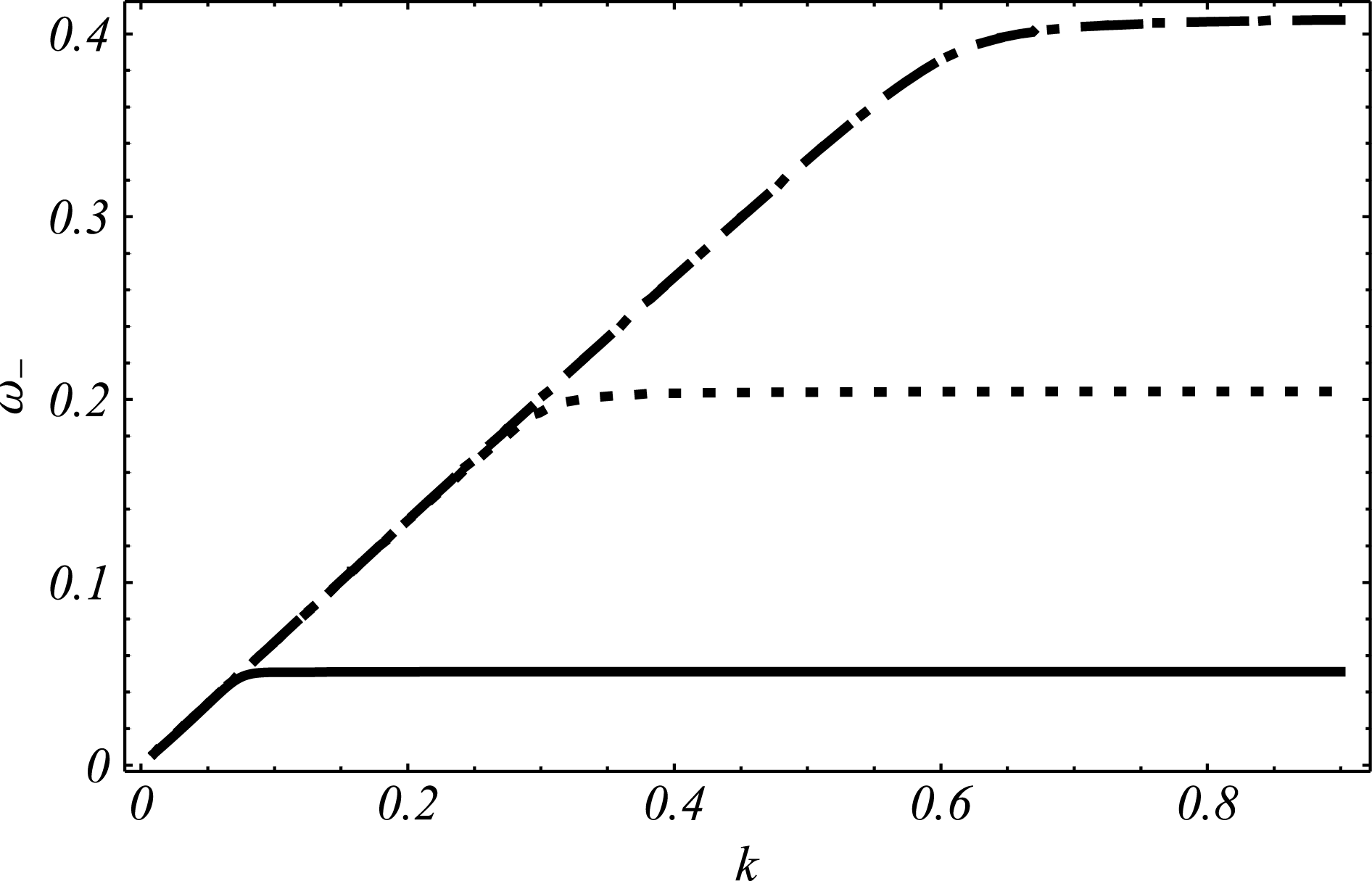
The low frequency mode of the electrostatic wave i.e.
 ${\it\omega}_{-}$
versus
 $k$
is plotted for different values of entropic indices i.e.
 $q_{e}$
,
 $q_{p}$
;
 $q_{e}=q_{p}=0.35$
(solid curve),
 $q_{e}=$
 $q_{p}=0.9$
(dotted curve),
 $q_{e}=q_{p}=2$
(dashed dotted curve). For the plasma
 ${\it\mu}=5$
,
 $p=4$
,
 $T_{e}=T_{p}=10^{3}~\text{K}$
,
 $T_{i}=0.2T_{e}$
,
 $k_{y}=0.1k_{x}$
and
 $B_{0}\sim 10^{2}~\text{G}$
.

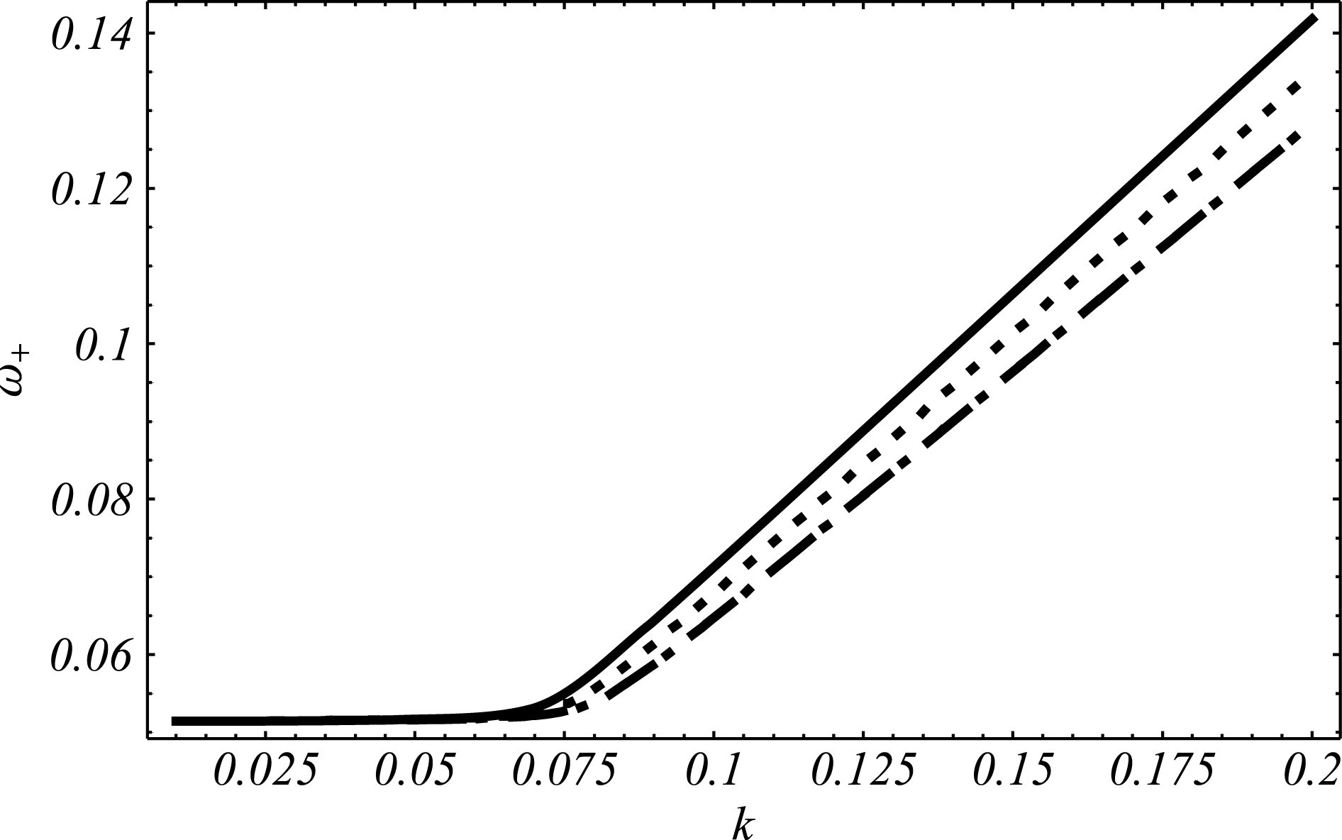
The high frequency mode of the electrostatic wave i.e.
 ${\it\omega}_{+}$
versus
 $k$
is plotted for different values of entropic indices i.e.
 $q_{e}$
,
 $q_{p}$
;
 $q_{e}=q_{p}=0.35$
(solid curve),
 $q_{e}=$
 $q_{p}=0.9$
(dotted curve),
 $q_{e}=q_{p}=2$
(dashed dotted curve). For the plasma
 ${\it\mu}=5$
,
 $p=4$
,
 $T_{e}=$
 $T_{p}=10^{3}~\text{K}$
,
 $T_{i}=0.2T_{e}$
,
 $k_{y}=0.1k_{x}$
and
 $B_{0}\sim 10^{2}~\text{G}$
.

The low frequency mode of the electrostatic wave i.e.
 ${\it\omega}_{-}$
versus
 $k$
is plotted for different values of magnetic field. The plasma parameters are
 ${\it\mu}=5$
,
 $p=4$
,
 $T_{e}=T_{p}=10^{3}~\text{K}$
,
 $T_{i}=0.2T_{e}$
,
 $k_{y}=0.1k_{x}$
,
 $q_{e}=q_{p}=0.9$
for
 $B_{0}=10^{2}~\text{G}$
(solid curve),
 $B_{0}=4\times 10^{2}~\text{G}$
(dotted curve),
 $B_{0}=8\times 10^{2}~\text{G}$
(dashed dotted curve).

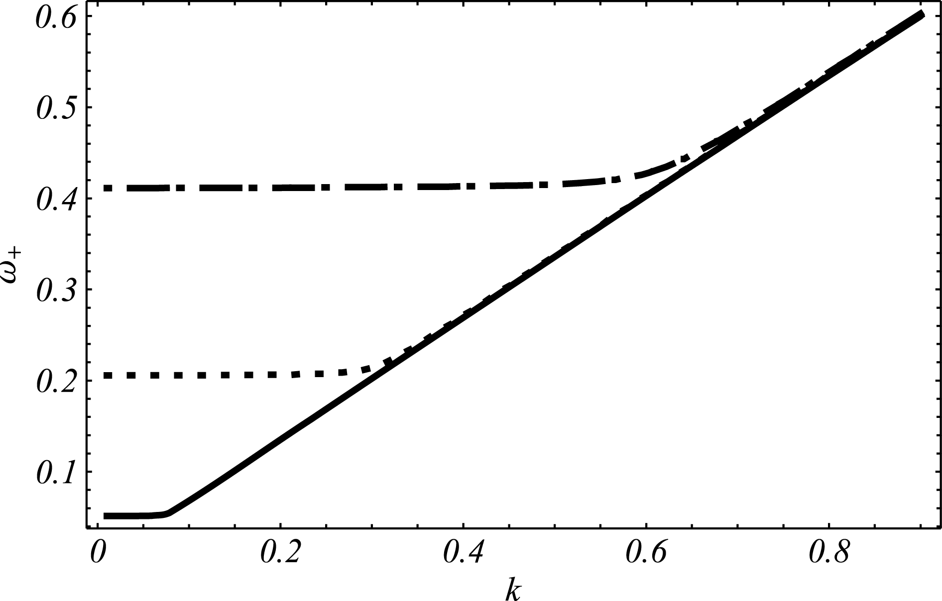
The high frequency mode of the electrostatic wave i.e.
 ${\it\omega}_{+}$
vs
 $k$
is plotted for different values of magnetic field. The plasma parameters are
 ${\it\mu}=5$
,
 $p=4$
,
 $T_{e}=T_{p}=10^{3}~\text{K}$
,
 $T_{i}=0.2T_{e}$
,
 $k_{y}=0.1k_{x}$
,
 $q_{e}=$
 $q_{p}=0.9$
for
 $B_{0}=10^{2}~\text{G}$
(solid curve),
 $B_{0}=4\times 10^{2}~\text{G}$
(dotted curve),
 $B_{0}=8\times 10^{2}~\text{G}$
(dashed dotted curve).

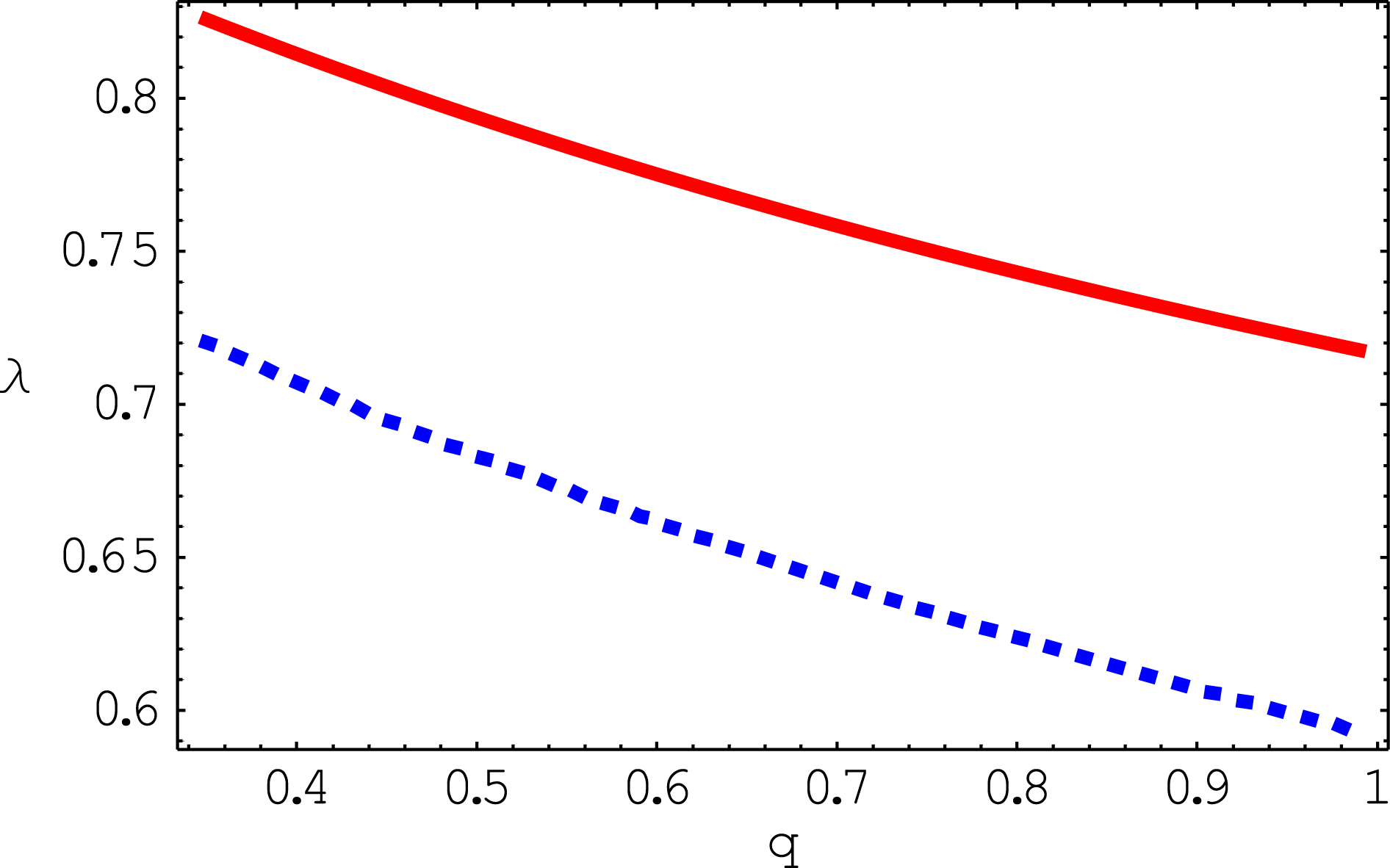
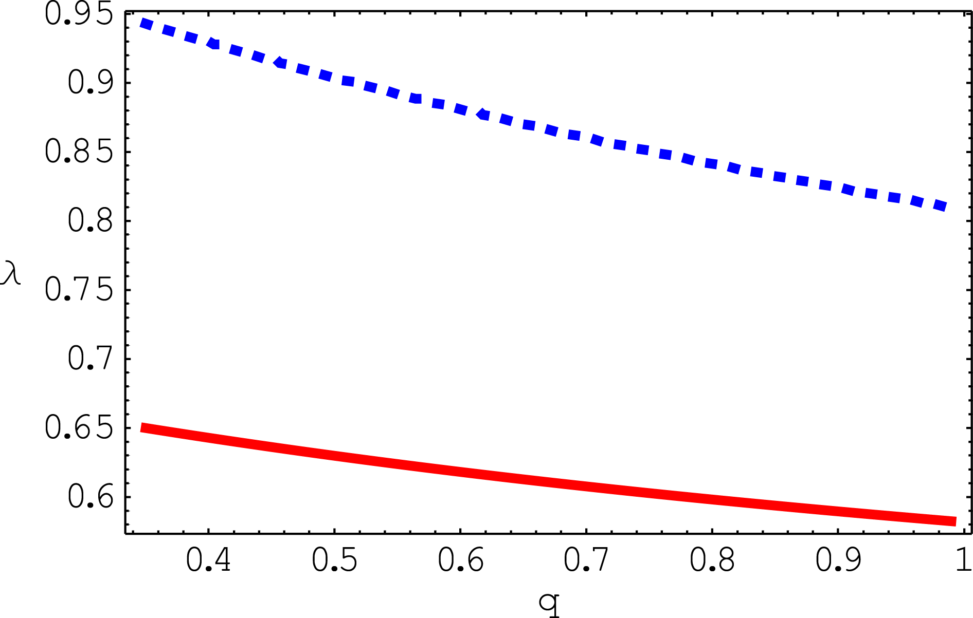
The phase velocity
 ${\it\lambda}$
is plotted for IA wave in EPI plasmas at different ion temperature (
 $T_{i}$
) against entropic indices
 $q_{e}$
,
 $q_{p}$
for the non-thermal electrons and positrons. The plasma parameters are
 ${\it\mu}=1.2$
,
 $p=0.2$
,
 $T_{e}=T_{p}=10^{3}~\text{K}$
for
 $T_{i}=0.2T_{e}$
(red solid curve),
 $T_{i}=0$
(blue dotted curve).

The phase velocity
 ${\it\lambda}$
is plotted for IA wave in EPI plasmas at different positrons density against entropic indices
 $q_{e}$
,
 $q_{p}$
for the non-thermal electrons and positrons. The plasma parameters are
 $T_{i}=0.2T_{e}$
,
 $T_{e}=T_{p}=10^{3}~\text{K}$
,
 $p=0.9$
(red solid curve),
 $p=0$
(blue dotted curve).

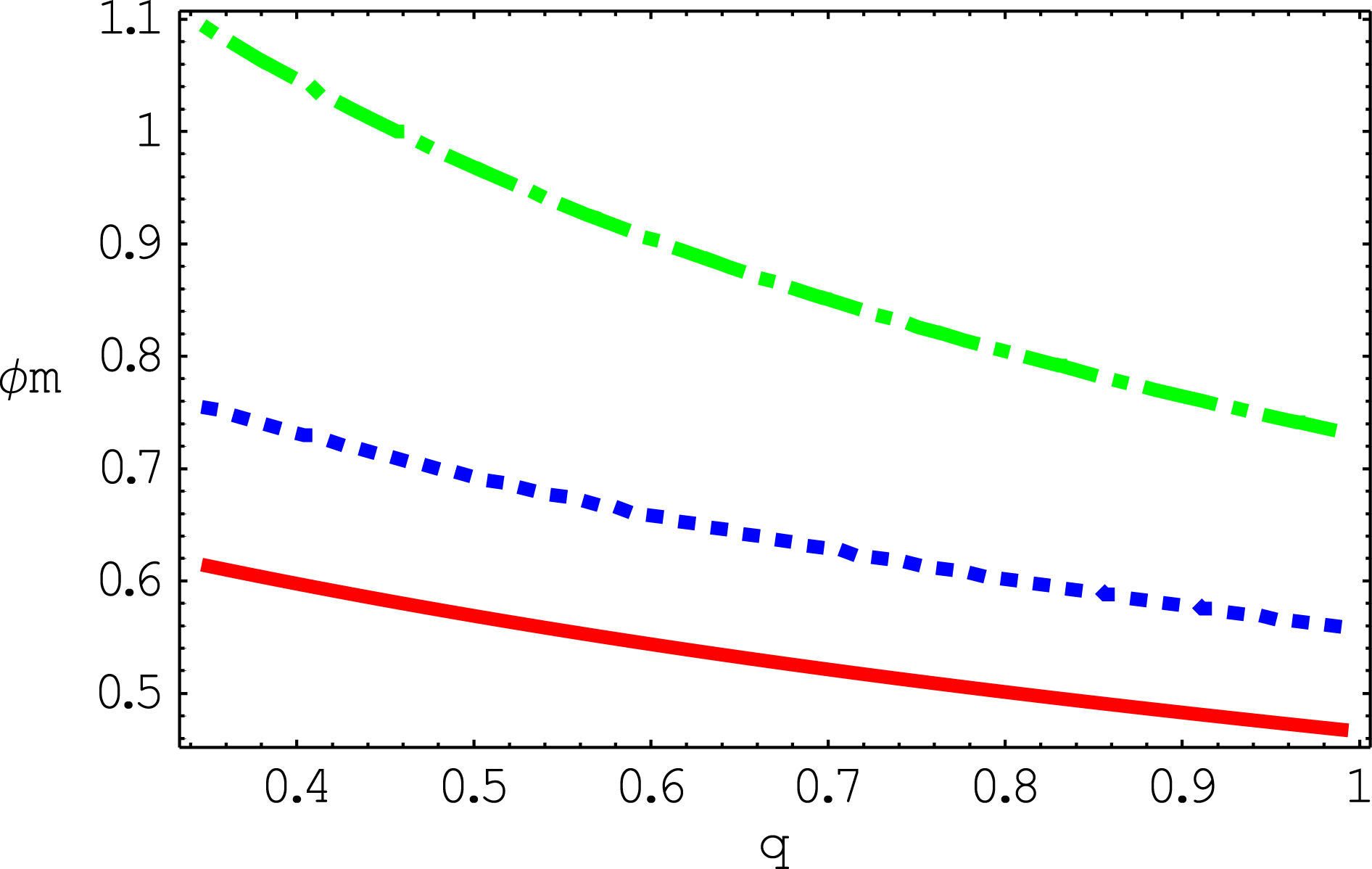
The IA soliton amplitude
 ${\it\phi}_{m}=\left(3u_{0}/A\right)$
is plotted for different values of positron density concentration and entropic indices
 $q_{e}$
,
 $q_{p}$
for the non-thermal electrons and positrons. The plasma parameters are
 $u_{0}=0.3$
,
 $T_{i}=0.2T_{e}$
,
 $T_{e}=T_{p}=10^{3}~\text{K}$
,
 $B_{0}\sim 10~\text{G}$
,
 $p=0.4$
(red solid curve),
 $p=0.2$
(blue dotted curve) and
 $p=0$
(green dashed dotted curve).

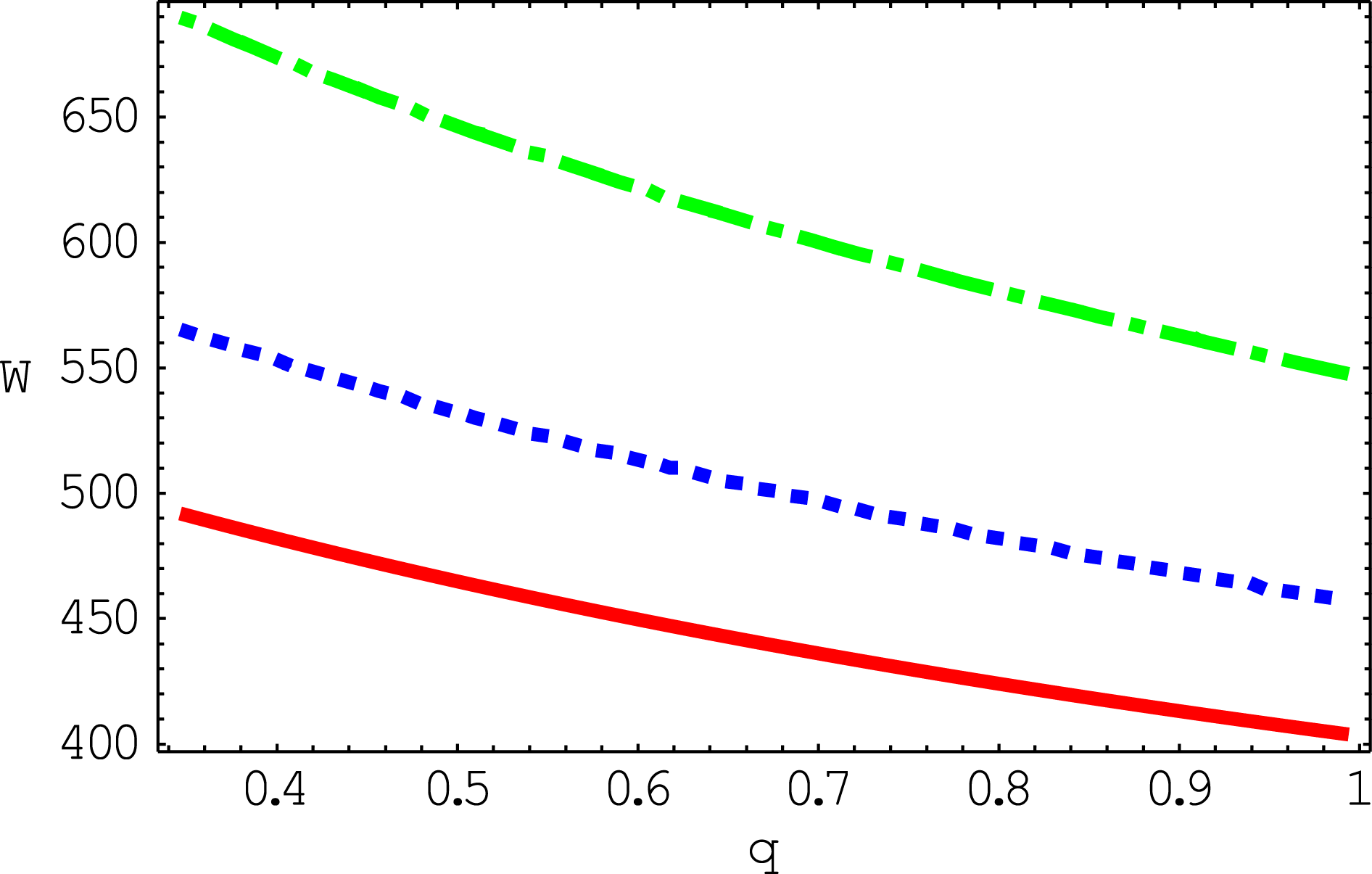
The width of the soliton
 $W=\sqrt{4(B+C)/u_{0}}$
is plotted for different values of positron density concentration and entropic indices
 $q_{e}$
,
 $q_{p}$
for the non-thermal electrons and positrons. The plasma parameters are
 $u_{0}=0.3$
,
 $T_{i}=0.2T_{e}$
,
 $T_{e}=T_{p}=10^{3}~\text{K}$
,
 $B_{0}\sim 10~\text{G}$
,
 $p=0.4$
(red solid curve),
 $p=0.2$
(blue dotted curve) and
 $p=0$
(green dashed dotted curve).

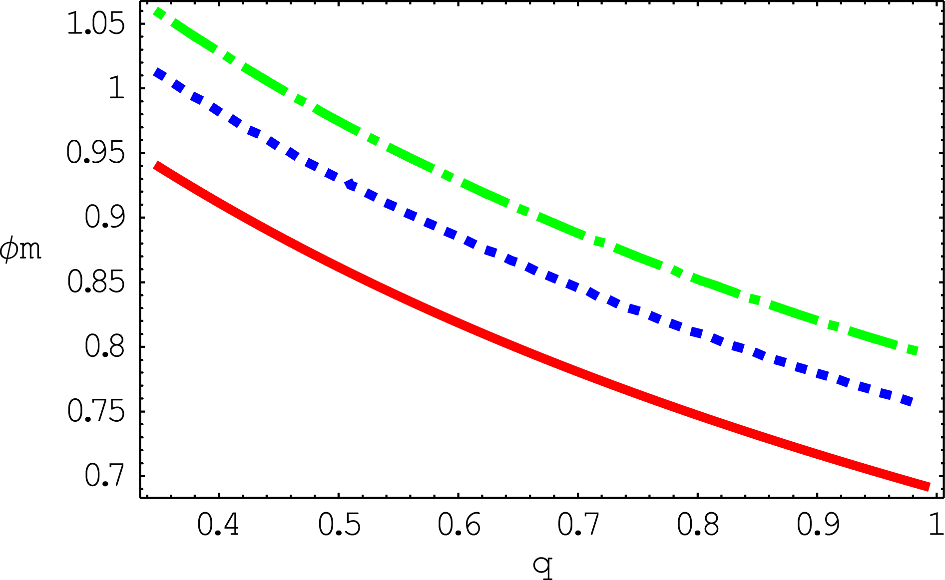
The amplitude of the soliton
 ${\it\phi}_{m}=(3u_{0}/A)$
is plotted against entropic indices
 $q_{e}$
,
 $q_{p}$
for the electrons and positrons for different values of
 ${\it\sigma}$
. The plasma parameters are
 $u_{0}=0.3$
,
 ${\it\mu}=1.2$
,
 $p=0.2$
,
 $T_{e}=T_{p}=10^{3}~\text{K}$
,
 $B_{0}\sim 10~\text{G}$
,
 $T_{i}=0.28T_{e}$
(red solid curve),
 $T_{i}=0.1T_{e}$
(blue dotted curve) and
 $T_{i}=0$
(green dashed dotted curve).

The soliton width
 $W=\sqrt{4(B+C)/u_{0}}$
is plotted against entropic indices
 $q_{e}$
,
 $q_{p}$
for the electrons and positrons for different values of
 ${\it\sigma}$
. The plasma parameters are
 $u_{0}=0.3$
,
 ${\it\mu}=1.2$
,
 $p=0.2$
,
 $T_{e}=T_{p}=10^{3}~\text{K}$
,
 $B_{0}\sim 10~\text{G}$
,
 $T_{i}=0.28T_{e}$
(red solid curve),
 $T_{i}=0.1T_{e}$
(blue dotted curve) and
 $T_{i}=0$
(green dashed dotted curve).

The width
 $W=\sqrt{4(B+C)/u_{0}}$
of the soliton is plotted for different values of magnetic field intensity
 $B_{0}$
against entropic indices
 $q_{e}$
,
 $q_{p}$
for the electrons and positrons. The plasma parameters are
 $u_{0}=0.3$
,
 ${\it\mu}=1.2$
,
 $p=0.2$
,
 $T_{e}=T_{p}=10^{3}~\text{K}$
,
 $T_{i}=0.2T_{e}$
,
 $B_{0}=0.1~\text{G}$
(red solid curve),
 $B_{0}=20~\text{G}$
(blue dotted curve) and
 $B_{0}=10^{2}~\text{G}$
(green dashed dotted curve).

4. Numerical illustrations and discussion
In this section we illustrate the characteristics and instability of two-dimensional IASW in magnetized EPI plasmas based on the results presented in §§ 3 and 4.
The variations of the planar solution,
 ${\it\varphi}_{0}$
, given by (3.15), in (a) and
 ${\it\psi}={\it\psi}_{0}+k{\it\psi}_{1}+\cdots \,,$
given by (3.18), in (b) versus
 ${\it\chi}$
where
 ${\it\nu}_{0}=2$
(black solid curve),
 ${\it\nu}_{0}=5$
(red dashed curve) and
 ${\it\nu}_{0}=8$
(blue dashed dotted curve). Here,
 $k=0.75$
.

The high and low frequency modes of the dispersion relation
 ${\it\omega}_{+,-}$
versus
 $k$
are plotted with variations of non-extensive parameter for electrons
 $q_{e}$
(same value for
 $q_{p}$
) and the magnetic field
 $B_{0}$
. In figures 1 and 2 the low (IA wave) and high (ion cyclotron wave) frequency modes of the dispersion relation are shown at different values of the non-extensive parameter i.e.
 $q_{e}$
. It can be seen from figure 1 that as we increase the values of
 $q_{e}$
, the saturation of the curve for the low frequency mode occurs at larger values of
 $k$
, while for the high frequency mode, saturation of the curves are created at small wavelengths or at large
 $k$
values as shown in figure 2. Magnetic field variation on the low and high frequency modes of the dispersion relation are presented in figures 3 and 4, respectively. The phase velocity of the low wave increases by enhancing the magnetic field strength while the saturation of the curve occurs at large values of
 $k$
shown in figure 3. The phase velocity of the high wave also increases with the increase in the magnetic field strength and the wave dispersion occurs at large
 $k$
values described in figure 4. The phase velocity of low or IAW (
 ${\it\lambda}$
) defined in (3.7) is plotted in figure 5 in EPI plasmas for different cases of ion temperature i.e.
 ${\it\sigma}$
(ratio of ion-to-electron temperature) and variations of entropic indices
 $q_{e}$
,
 $q_{p}$
for the non-thermal electrons and positrons. It is found that the phase velocity of IA wave is decreased with an increase of entropic indices i.e.
 $q_{e}$
,
 $q_{p}$
for the electrons and positrons. The phase velocity of IA wave increases in the presence of an ion temperature in comparison with the cold ions case (i.e.
 ${\it\sigma}=0$
) for
 $q_{e}$
,
 $q_{p}>0$
. In figure 6 phase velocity,
 ${\it\lambda}$
, is plotted for the different positron concentrations versus entropic indices i.e.
 $q_{e}$
,
 $q_{p}$
for the electrons and positrons, respectively. The phase velocity,
 ${\it\lambda}$
, is larger in the presence of positrons in comparison with the absence of a positron concentration as shown in the figure. It is noticed that the phase velocity of the IA wave decreases with the increase in the value of entropic indices i.e.
 $q_{e}$
,
 $q_{p}$
for the electrons and positrons keeping positron concentration fixed. The amplitude of the soliton
 ${\it\phi}_{m}=(3u_{0}/A)$
is plotted in figure 7 for different values of positron concentration against the entropic indices of electrons and positrons. The amplitude of the IA soliton increases as we decrease the positron concentration, keeping all others parameters fixed. The width of the soliton
 $W=\sqrt{4(B+C)/u_{0}}$
is plotted in figure 8 for all the same parameters used in figure 7, and we found a similar trend. The width of the soliton decreases at larger values of positron concentration and non-extensive parameter. The amplitude of the soliton is plotted in figure 9 for different values of ion temperature and entropic indices
 $q_{e}$
,
 $q_{p}$
. The amplitude of the soliton decreases for the larger values of
 ${\it\sigma}$
and entropic indices
 $q_{e}$
,
 $q_{p}$
. The soliton width
 $W$
is plotted for the temperature coefficient
 ${\it\sigma}$
in figure 10. The width of the soliton increases for large values of
 ${\it\sigma}$
and vice versa for the non-extensive parameters. The width for the ion acoustic wave in EPI is plotted for the magnetic field intensity. It can be seen that there is no change in the amplitude, whereas the width of the soliton reduces significantly with the increase in magnetic field strength i.e.
 $B_{0}$
(0.1 G, 20 G, 100 G) as shown in figure 11. It is also evident from (3.10) that the intensity of the external magnetic field
 $B_{0}$
has no direct effect on the amplitude of the solitary waves. The contribution of the ion gyro-frequency
 ${\it\Omega}$
comes into play on the width of the soliton through the coefficient
 $C$
in (3.9). The amplitude of the soliton remains the same while the width decreases with increasing
 ${\it\Omega}$
i.e. a stronger magnetic field leads to steeper and thus narrower soliton profiles, which agrees with the results of Sultana et al. (Reference Sultana2010). Figure 12 shows the variation of the planar solution,
 ${\it\varphi}_{0}$
, that is given by (3.15), and the function
 ${\it\psi}={\it\psi}_{0}+k{\it\psi}_{1}+\cdots \,$
appears in the perturbed solution; (3.18) against
 ${\it\chi}$
and different values of
 ${\it\nu}_{0}.$
It is clear that
 ${\it\varphi}_{0}$
(
 ${\it\psi}$
) decreases (increases) as
 ${\it\chi}$
increases (decreases). For
 ${\it\chi}<1,{\it\varphi}_{0}$
increases as
 ${\it\nu}_{0}$
increases. The opposite effect is observed where
 ${\it\chi}>1$
. Since,
 ${\it\varphi}_{0}$
changes its behaviour with
 ${\it\nu}_{0}$
at
 ${\it\chi}=1,$
this
 ${\it\psi}$
-corresponding characteristic point occurs at
 ${\it\chi}\simeq 1.75$
. Moreover, the variation curves of
 ${\it\psi}$
versus
 ${\it\chi}$
shows the existence of minimum points appearing at smaller
 ${\it\chi}$
by increasing
 ${\it\nu}_{0}$
. Figure 12 proves that there are some points at which
 $|{\it\psi}|>|{\it\varphi}_{0}|$
that may lead to instability of the produced solitons in the transverse direction (comparing the dash dotted curves in the two panels that correspond to higher values of
 ${\it\nu}_{0}$
).
5. Conclusion
To conclude, we have studied the nonlinear IASW in magnetized EPI plasmas. The electrons and positrons follow the
 $q$
-non-extensive distribution while the ions are taken to be warm and inertial. By using the well-known RPM, we drive a ZK equation. The solution to the ZK equation is analysed for different parameters i.e.
 $q_{e}$
,
 $q_{p}$
,
 $B_{0}$
,
 ${\it\sigma}$
,
 $p$
. It is evident that the non-extensive parameters
 $q_{e}$
,
 $q_{p}$
, positron concentration ratio
 $p$
and the ion-to-electron temperature ratio
 ${\it\sigma}$
effect on both the amplitude and the width of the soliton, whereas the magnetic field
 $B_{0}$
affects only the soliton width. The instability analysis reveals that the one-dimensional soliton solution suffers from an instability in the transverse direction. The instability growth rate of the IASW is a constant, cf. (3.32). Our theoretical results may be applied to systems with long-range interactions, such as space and astrophysical magnetized plasmas containing non-thermal electrons, positrons and warm ions.