1. Introduction
A bubble expanding and collapsing close to a solid boundary has been attracting attention in engineering and biomedical research. Overall, the cavitation phenomenon may be used for benefit but could also cause harm to nearby structures. On the positive side of applications are ultrasonic cleaning (Chahine et al. Reference Chahine, Kapahi, Choi and Hsiao2016), non-invasive surgery (Bismuth et al. Reference Bismuth, Eck and Ilovitsh2023) and ice breaking (Cui et al. Reference Cui, Zhang, Wang and Khoo2018) to name a few, while negative effects include cavitation damage to flow structures such as pump blades (Lu et al. Reference Lu, Tan, Han and Liu2022) and ship propellers (Arveson & Vendittis Reference Arveson and Vendittis2000). There is growing research interest in controlling the fluid mechanics of cavitation bubble collapse near solid boundaries to mitigate these negative effects (Kim & Kim Reference Kim and Kim2020). When the cavitation bubble collapses close to a flat rigid boundary, the cavitation bubble translates towards the boundary and develops a microjet pointing to the boundary (Lauterborn & Bolle Reference Lauterborn and Bolle1975; Lindau & Lauterborn Reference Lindau and Lauterborn2003; Reuter & Mettin Reference Reuter and Mettin2018; Sun et al. Reference Sun, Du, Yao, Zhong, Geng and Wang2022). In contrast, near a free surface the bubble is moving away resulting in a microjet that is repelled from the free surface (Krieger & Chahine Reference Krieger and Chahine2005; Gong et al. Reference Gong, Ohl, Klaseboer and Khoo2010; Zhang et al. Reference Zhang, Wang and Zhang2016; Supponen Reference Supponen2017). This led to vivid research on the effect of various kinds of boundaries (Brujan et al. Reference Brujan, Noda, Ishigami, Ogasawara and Takahira2018; Andrews et al. Reference Andrews, Rivas and Peters2020, Reference Andrews, Fernández Rivas and Peters2023; Rodriguez et al. Reference Rodriguez, Beig, Barbier and Johnsen2022; Li et al. Reference Li, Zhang, Cui, Li and Liu2023; Zhang et al. Reference Zhang, Li, Xu, Pei, Li and Liu2024). The free surface combined with the rigid wall (Huang et al. Reference Huang, Zhang, Ma, Chang, Zheng and Huang2020) and the bubbles attached to the boundary are studied (Wang et al. Reference Wang, Liu, Yuan, Jiang and Wang2020; Goh et al. Reference Goh, Ohl, Klaseboer and Khoo2014). While the microjet has been considered in the past as a cause for cavitation damage, more recent research has revealed single bubbles collapsing in direct contact with the surface that erode the surface through shock wave amplification (Reuter et al. Reference Reuter, Deiter and Ohl2022a ). A viable strategy to reduce damage would be to reduce either the strength of the collapse or increase its distance from the boundary. (Kiyama et al. Reference Kiyama, Shimazaki, Gordillo and Tagawa2021; Guo et al. Reference Guo, Zhang, Lei and Galindo-Torres2022; Rosselló et al. Reference Rosselló, Reese and Ohl2022; Yong et al. Reference Yong, Yang, Huo, Hou and Chen2022). To understand the effect of non-trivial boundaries, i.e. such that have topographical features, one may utilise the Kelvin impulse model to predict the motion of the cavitation bubble and the resulting microjet (Benjamin & Ellis Reference Benjamin and Ellis1966; Blake & Gibson Reference Blake and Gibson1981, Reference Blake and Gibson1987; Blake Reference Blake1988; Blake et al. Reference Blake, Leppinen and Wang2015; Xu et al. Reference Xu, Li, Ren, Liu and Zuo2023). The Kelvin impulse is widely used in characterizing various physical quantities of bubbles and is closely connected to the anisotropy parameter introduced by Obreschkow et al. (Reference Obreschkow, Tinguely, Dorsaz, Kobel, de Bosset and Farhat2011), Supponen (Reference Supponen2017) and Sieber et al. (Reference Sieber, Preso and Farhat2022). In the present work, we investigate the dynamics of laser-induced cavitation bubbles near a gas-entrapping rigid surface experimentally, numerically and analytically. To study the bubble interactions, we selected eight different hole sizes. We first introduce the experimental set-up, then report on the experimental results before we introduce the Kelvin impulse model for our particular geometry. Additionally, we utilise a volume of fluid (VoF) solver (OpenFOAM) to model the compressible and viscous bubble dynamics close to the gas-entrapping rigid surface. This allows us to classify the jet dynamics into three different regimes and compare the bubble’s oscillation periods, displacements and the velocities of their microjets.
2. Experimental set-up
The experimental set-up is shown in figure 1, and it consists of three parts: a laser to generate single cavitation bubbles; a high-speed camera to record the bubble dynamics; and a pulse delay generator used for controlling the timing. A metal hollow block (30
 $\times$
32
 $\times$
30 mm
 $^3$
) is placed in the water tank (50
 $\times$
100
 $\times$
50 mm
 $^3$
) that is filled with air and has a small opening, which traps the gas–liquid interface. A Nd:YAG laser (Grace Laser TINY-L, wavelength 1064 nm, maximum energy 120 mJ and pulse duration 6 ns) is used to generate bubbles. The initial laser beam width is 5.6
 $\rm mm$
and first expanded into 16.8
 $\rm mm$
by a beam expander (
 $3 \times$
expansion ratio, GCO25 model from Daheng Optics, China) and then focused with a lens (
 $f=25\,$
mm, NA = 0.5) to induce a cavitation bubble in water. The position of the laser is adjusted with the help of a green pilot laser beam such that the cavitation bubble is generated aligned with the centre of the gas-entrapping hole. A bright light source (Danny U U-100T) illuminates the volume to record the dynamics of the bubble with a high-speed camera (Phantom TMX7510, 230 000 fps or frame interval of 4.35 μs). The triggers for the flashlamp and Q-switch of the laser and the trigger signal of the camera are controlled with a pulse delay generator (DDPG, Quantum composers 9528). The energy of the laser and thus the bubble size is adjusted by the time interval between the flashlamp and the Q-switch trigger. The start of the recording of the bubble is set by the time interval between the Q-switch trigger and the camera trigger.
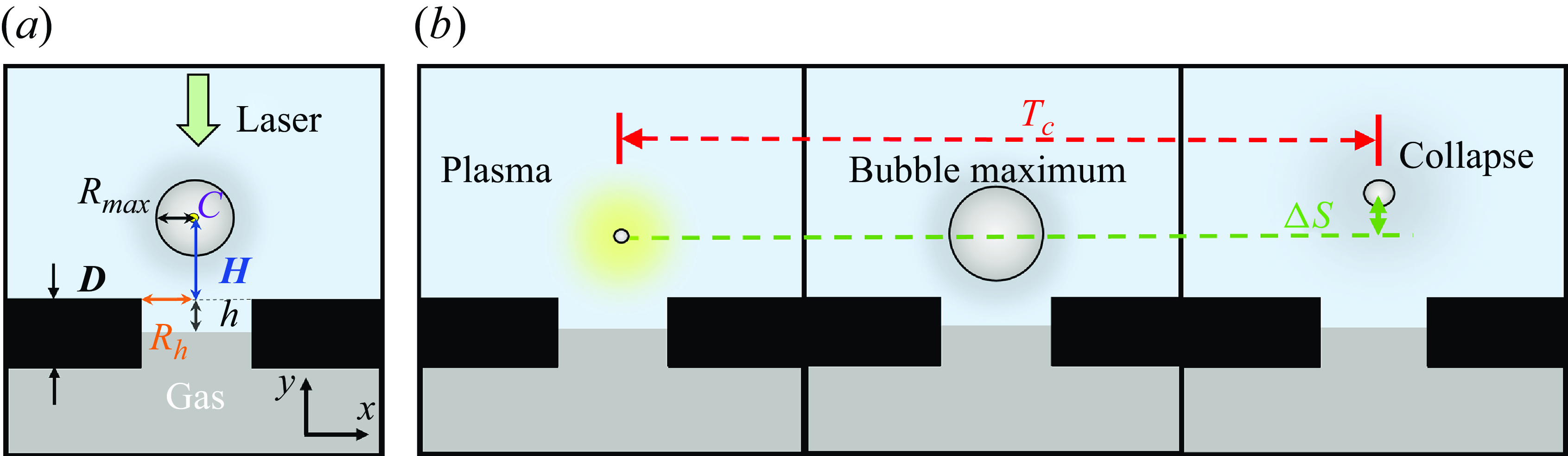
The experimental set-up to generate and observe a laser-induced cavitation bubble. The laser pulse is expanded and then focused from outside the cuvette with a lens close to the submerged structure.

The experimental parameters depicted in (a) are the bubble maximum radius
 $R_{\textit{max}}$
 $\approx$
1.0 mm, the bubble centroid
 $C$
position, the radius of the gas-entrapping hole
 $R_h$
, the distance from plasma to the rigid surface
 $H$
and the wall thickness
 $D$
is maintained constant at 2 mm. The height of interface
 $h$
is from the rigid wall to the topper of interface. (b) Here
 $T_c$
is the time between bubble generation and first collapse. Here
 $\Delta S$
is the bubble centroid displacement from the plasma centroid to the location of the first bubble collapse.

Important experimental parameters are sketched in figure 2. The bubble expands from an initial plasma, reaches its maximum radius, shrinks under the action of the ambient pressure and collapses into a minimum size. This duration from generation to final collapse is defined as the period of the bubble oscillation,
 $T_c$
. The distance from the plasma centroid to the location of collapse is the displacement of the bubble,
 $\Delta S$
. In the presented experiments, the energy of the laser is fixed resulting in bubbles with maximum radius
 $R_{\textit{max}}$
of approximately 1.0
 $\rm mm$
. The vertical distance from the plasma to the rigid surface trapping the gas is
 $H$
. The gas-entrapping hole is circular with radius
 $R_h$
. We vary the holes as 0.0, 0.50, 0.75, 1.00, 1.25, 1.50, 1.75 and 2.00
 $\rm mm$
. The experimental results can then be expressed by the dimensionless parameters stand-off distance
 $\gamma$
=
 $H$
/
 $R_{\textit{max}}$
and hole size parameter
 $\alpha$
=
 $R_{h}$
/
 $R_{\textit{max}}$
. The range for
 $\gamma$
is between 0.5 and 3.2, and for
 $\alpha$
is between 0 and 2.0. Each group of experiments was repeated five times. The interval
 $T_{\textit{sd}}=2T_{c}^{Rayleigh}=0.915 R_{\textit{max}}\sqrt {\rho /\Delta p}$
(Rayleigh Reference Rayleigh1917) is the time that is twice the Rayleigh collapse time, i.e. the time to close a cavity with radius
 $R_{\textit{max}}$
in an unbounded liquid. Here, the non-dimensional buoyancy parameter
 $F$
(Zhang et al. Reference Zhang, Cui, Cui and Wang2015) compares the hydrostatic pressure with the pressure difference driving the bubble collapse:
 $F= \sqrt {\rho g R_{\textit{max}}/\Delta p}$
. In our experiment, we obtain
 $F\sim 0.01$
for
 $\rho =1000\,\rm kg\,m^-{^3}$
,
 $g=9.8\,\rm ms^-{^2}$
,
 $R_{\textit{max}}=1\,$
mm and
 $\Delta p=1\,$
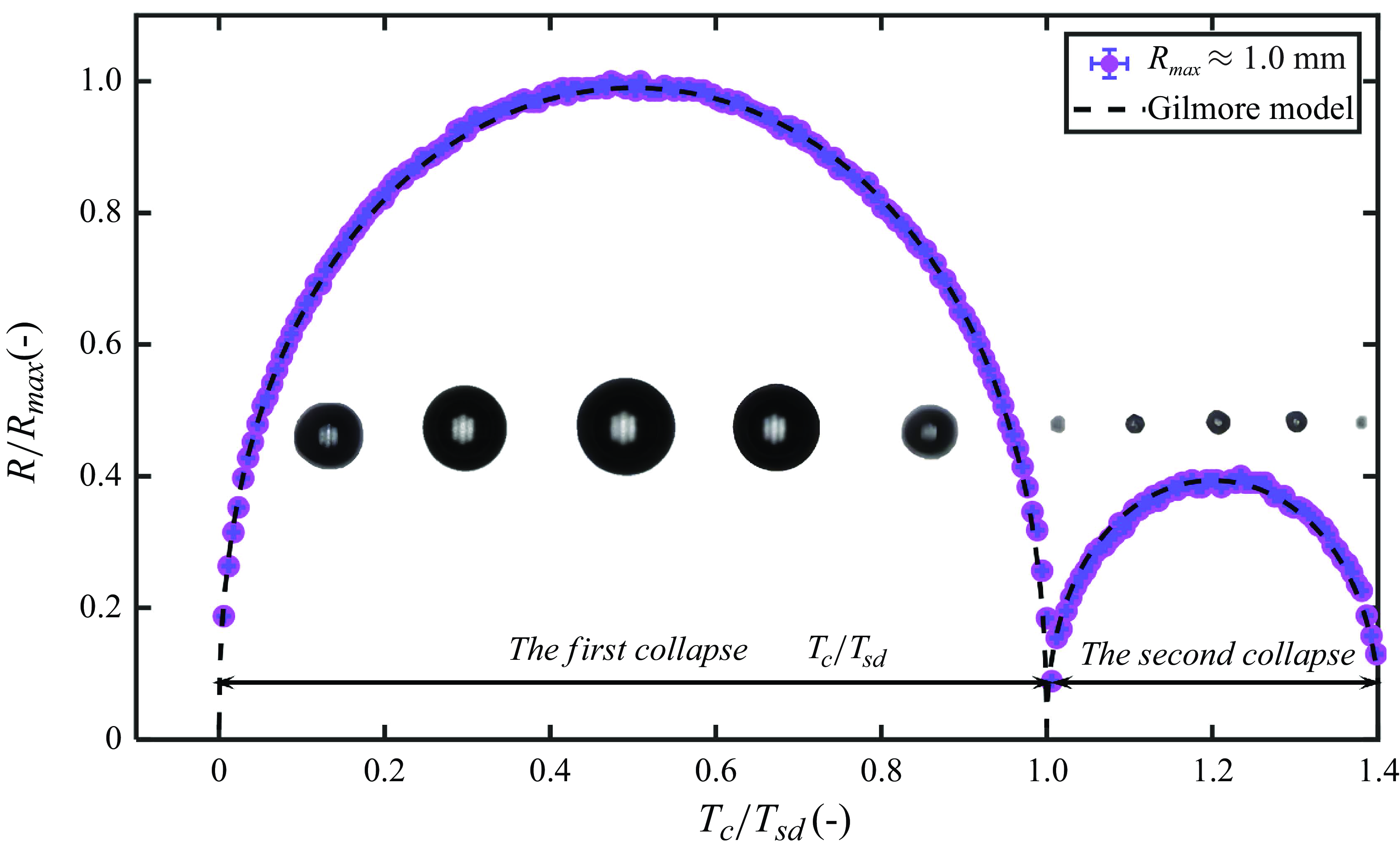
bar. Thus, buoyancy can be safely ignored in the present experiments. To ensure the repeatability and accuracy of laser-induced bubbles, we first observed that the evolution far away from boundaries simulate an approximately infinite fluid. In absence of boundaries, buoyancy and an ideal spherical laser plasma the bubble should remain spherical. Figure 3 shows the evolution of the dimensionless radius of the bubble
 $R$
/
 $R_{\textit{max}}$
with dimensionless time
 $T$
/
 $T_{sd}$
. Selected frames from the high-speed recording of the bubble are added. The symbols are the extracted radii from the high-speed images and the dashed line is taken from the solution of the Gilmore model (Lauterborn & Kurz Reference Lauterborn and Kurz2010) showing a good agreement.
The evolution of bubble in approximate infinite fluid is compared with the Gilmore model using the parameters for water. In Gilmore model (Lauterborn & Kurz Reference Lauterborn and Kurz2010), the initial bubble radius
 $R_{0}$
= 0.04 mm,
 $\sigma$
= 0.07 Nm–1,
 $B$
= 314 MPa and
 $n_{T}$
= 7 in Tait,
 $k$
= 3/4 and
 $b$
= 0 for the van der Waals law.

2.1. Analytical model
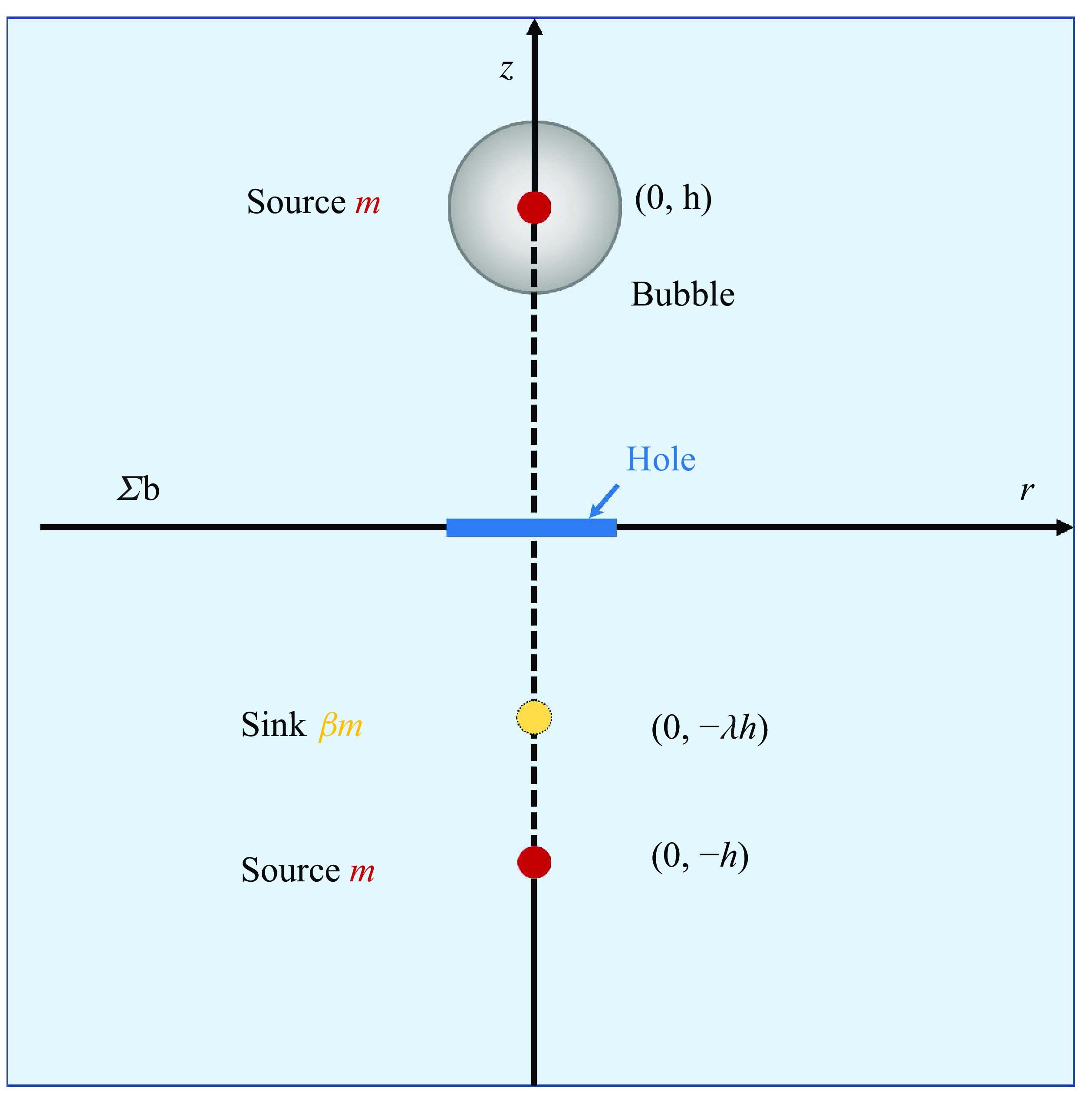
The Kelvin impulse is derived from potential flow theory to quantify the bubble motion (Benjamin & Ellis Reference Benjamin and Ellis1966; Blake & Gibson Reference Blake and Gibson1987; Blake et al. Reference Blake, Leppinen and Wang2015). The dynamics of a cavitation bubble near a gas-entrapping rigid surface is modelled with the method of images using two-point sources with a strength of
 $m$
and a point sink with reduced strength
 $\beta m$
placed at various distances before and behind the boundary, see figure 4. The image source accounts for the rigid boundary and the image sink for the free boundary of the hole. The relative size between the bubble and the hole affects the location and strength of the sink through the following two relationships. These two expressions are derived from the ‘S’ curve model (Panik Reference Panik2014), see Appendix A,
 \begin{equation} \lambda =1-e^{-0.83\alpha }, \end{equation}
 \begin{equation} \beta =2-2/(1+(\alpha /1.5)^{2}). \end{equation}
The schematic of the source–sink system. The red point is the source and the yellow the sink,
 $m$
is source strength. We place two sources, each with an intensity of
 $m$
, at the coordinates (0,
 $h$
), (0, –
 $h$
), respectively. We then put a sink with an intensity of
 $\beta m$
at the coordinate (0, –
 $\lambda h$
).

Figure 4 The schematic of the source–sink system, red point is source and yellow sink,
 $m$
is source strength. We place two sources, each with an intensity of
 $m$
, at the coordinates (0,
 $h$
), (0, -
 $h$
), respectively, and then put a sink with an intensity of
 $\beta m$
at the coordinate (0,
 $-\lambda h$
). From this potential-flow model we can derive the Kelvin impulse
 $I$
, (2.3), for a gas-entrapping rigid surface, see Appendix A for the derivation; the sign of the Kelvin impulse is only controlled by
 $\lambda$
and
 $\beta$
as the kernel of the integral is always positive,
 \begin{equation} I = \frac {\rho \left ( 4\beta /(\lambda +1)^2 - 1\right )}{16\pi h^2} \int _{-T_{c}^{Rayleigh}}^{T_{c}^{Rayleigh}} m^2 {\rm d}t .\end{equation}
A positive Kelvin impulse (
 $I\gt$
0) results in a bubble that moves in the positive
 $z$
-direction away from the boundary, and a negative Kelvin impulse causes the bubble to move towards the boundary. For
 $I$
= 0, no centre of mass motion is observed. In the limit of
 $\lambda$
= 0,
 $\beta$
= 0, (2.3) describes a rigid wall and for
 $\lambda$
= 1,
 $\beta$
= 2 a free surface. For all other values, a gas-entrapping rigid wall is modelled. Supponen (Reference Supponen2017) utilised the Kelvin impulse to define an anisotropy parameter
 $\zeta$
that allows comparison of the jetting of bubbles in different environments. For example, they derived an anisotropy parameter (2.4) for a bubble near a free surface (positive
 $\zeta$
-values) and for one close to a rigid wall (negative
 $\zeta$
-values):
 \begin{equation} \zeta =\pm 0.195\gamma ^{-2}. \end{equation}
If we follow their definition, we obtain for the present geometry an anisotropy parameter, (2.5); for the derivation, see Appendix A,
 \begin{equation} \zeta = 0.195(4\beta /(\lambda +1)^2-1)\gamma ^{-2}. \end{equation}
3. Results and discussion
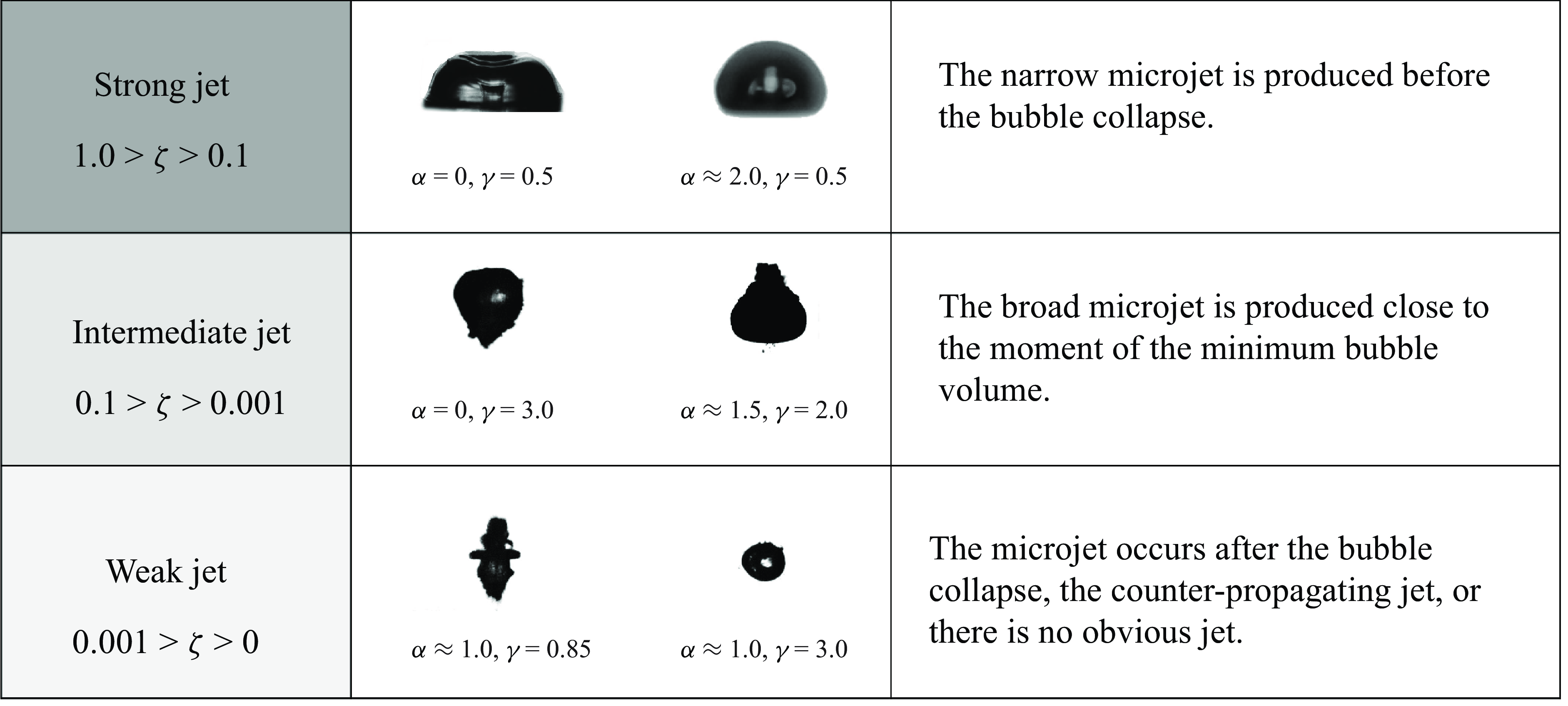
The microjet dynamics may be characterised into ‘strong’, ‘intermediate’ and ‘weak’, as a function of the strength of the anisotropy parameter
 $\zeta$
. We follow Supponen (Reference Supponen2017) where they divided the microjet into three types: weak jets hardly pierce the bubble, but remain within it throughout the collapse and rebound; intermediate jets pierce the opposite bubble wall close to the last collapse phase and clearly emerge during the rebound; strong jets pierce the bubble early during the collapse. Figure 5 depicts examples of these three kinds of jets. A strong jet (1.0
 $\gt \zeta \gt$
0.1) develops in the early stages of the bubble collapse phase and forms when the bubble is close to the boundary. The intermediate jet (0.1
 $\gt \zeta \gt$
0.001) occurs during the late stage of bubble collapse, and the jet will penetrate the bubble wall. In the present experiments, we find two situations for a weak jet (0.001
 $\gt \zeta \gt$
0) either from two counter-propagating jets or a single non-penetrating jet. The
 $\zeta$
-value approaching 0 means that the bubble does not translate during collapse or the bubble forms jets of similar strength in both directions to ensure the conservation of momentum. Other geometries resulting in an hourglass shape are two rigid boundaries (sample of publications) and a recent publication demonstrating it for two free boundaries (Zevnik et al. Reference Zevnik, Patfoort, Rosselló, Ohl and Dular2024). In the following, we will present the three kinds of jetting separately and discuss the mechanisms causing them in detail.
Three distinct microjet types: strong jet (1.0
 $\gt \zeta \gt$
0.1) seen early during the collapse; intermediate jet (0.1
 $\gt \zeta \gt$
0.001) emerging during the rebound; weak jet (0.001
 $\gt \zeta \gt$
0), the microjet flows towards both ends, or no obvious microjet penetrates the bubble wall.

3.1. Overview and classification of bubble dynamics
We now present an overview on the bubble dynamics by varying
 $\gamma$
and
 $\alpha$
to compare the experiments with the analytical model for the first bubble oscillation only. We use the analytical model to predict the strength of the jet and direction of the bubble. After inserting
 $\alpha$
into (A5) and (A6) we can obtain the direction of the bubble from (2.3). Additionally, we calculate the anisotropy parameter
 $\zeta$
. Figure 6 is a parameter plot for the variables (
 $\alpha$
,
 $\gamma$
) comparing the strength and the direction of the experimental jet (symbols) with the anisotropy parameters,
 $\zeta$
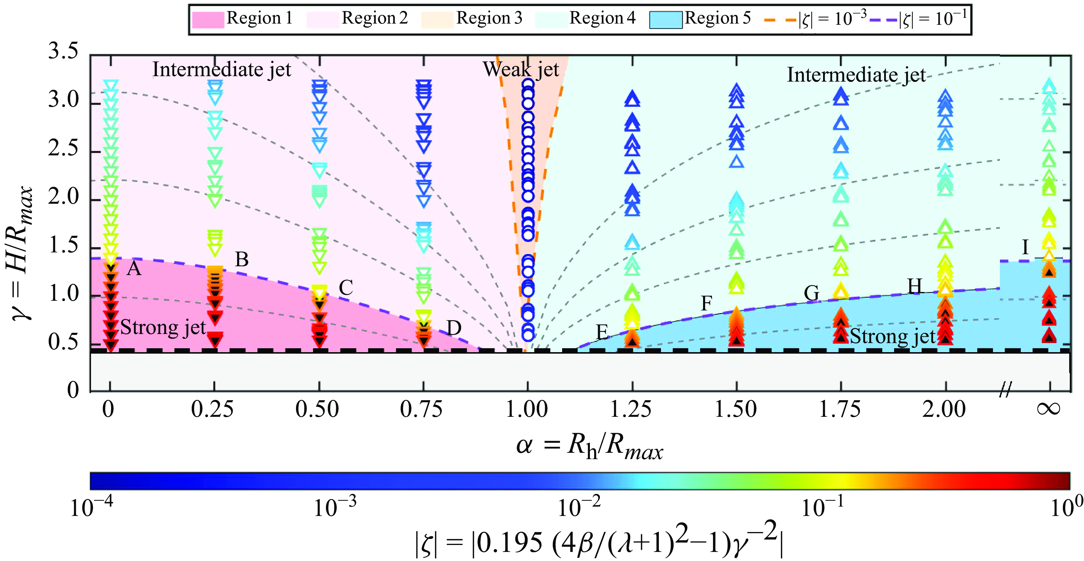
, from the analytical model. Downward triangles are bubbles collapsing towards the hole and the upward triangles away from it. The circle symbol is used for experiments where no jet or two counter-propagating jets are found. The strength of
 $\zeta$
is encoded in colours in figure 6. Overall, we find that the Kelvin impulse and the anisotropy parameter
 $\zeta$
are strong functions of the distance from the boundary. As
 $\gamma$
increases, this value decreases, indicating a reduction in the system momentum between the bubble and the boundary, leading to a weakening of bubble motion. Note that the direction of motion of the jet is considered only within the first oscillation period. At the same time, based on the movement and strength of the microjet, five regions are identified and will now be described in detail.
Parameter plot of jetting for (
 $\alpha$
,
 $\gamma$
). Symbols are from experiments and lines from the analytical model. Upward triangles show jetting away from the hole and downward triangles towards the hole. Filled triangles indicate strong jets and open symbols intermediate jets. Circles are from experiments with no centre of mass movement. The colour of the symbols is encoded by the value of the anisotropy parameter
 $\zeta$
. The five identified regions are discussed below. The orange and purple dashed lines represent
 $\zeta$
= 0.1 and 0.01, respectively, and the grey dashed lines are constant
 $\zeta$
with 0.2, 0.04, 0.02, 0.01 (from bottom to top).

3.1.1. Regions 1 and 2: downward jet
In regions 1 and 2, the opening of the gas-entrapping hole is smaller than the cross-sectional area of the bubble (
 $\alpha \lt$
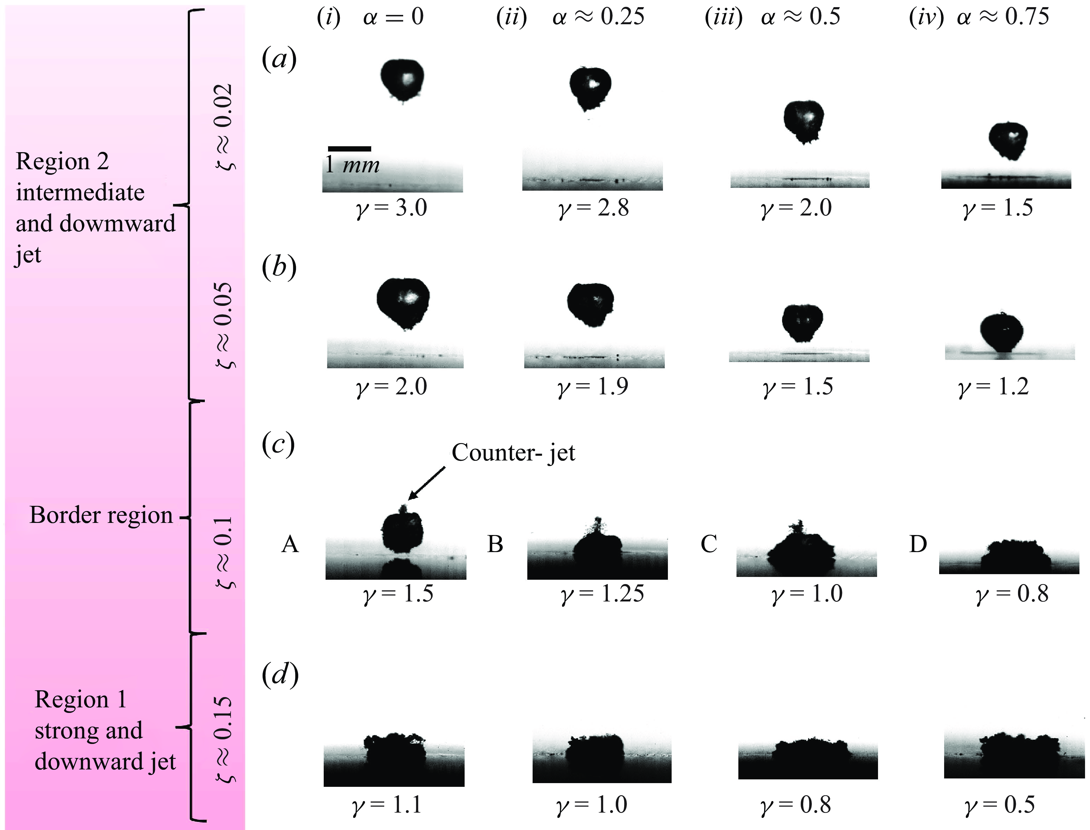
1.0). For these small hole sizes, let us compare the dynamics with that of a bubble near a rigid wall. There during shrinkage of the bubble the pressure at the upper pole of the bubble is higher than at the lower pole, which is due to the hindrance of the radial flow by the rigid boundary. This pressure gradient accelerates the upper bubble interface towards the wall developing a downward-directed jet through the centre of the bubble. In figure 7, four groups of bubble shapes with approximately equal
 $\zeta$
-value from the regions 1, 2 and the border region are depicted. Each group consists of four representative images captured five frames after the collapse event where the distance between the bubble and the boundary increases from left to right. The leftmost frame depicts the rigid wall case, while the three frames to the right show bubbles in the presence of holes that increase in diameter from left to right. It becomes evident that the bubble shape at collapse is governed strongly by the
 $\zeta$
-value and the shapes for the same
 $\zeta$
-value are rather similar. For
 $\zeta$
 $\approx$
0.15, the bubble obtains approximately a cylindrical shape due to the proximity to the wall. As
 $\zeta$
 $\approx$
0.1, the border region, the bubble loses this cylindrical shape and makes a broader contact with the boundary. For the rigid wall case, a prominent structure pointing upwards that was called the counter-jet becomes apparent (Lindau & Lauterborn Reference Lindau and Lauterborn2003). This counter-jet-like structure is also found in the presence of a hole. Interesting numerical simulations for rigid walls do not predict a counter-jet (Popinet & Zaleski Reference Popinet and Zaleski2002; Li et al. Reference Li, Zhang, Han and Liu2017; Lechner et al. Reference Lechner, Lauterborn, Koch and Mettin2020). The inability to model the counter-jet is consistent with the hypothesis that the counter-jet is rather a region of secondary cavitation than a liquid or gaseous flow. It is the result of a rarefaction wave that is generated during bubble collapse with a sufficiently wide jet. The contact area gradually diminishes with an increase in
 $\alpha$
. This phenomenon primarily stems from the enlargement of gas-entrapping holes, resulting in an increased free surface that impedes bubble–wall contact. When
 $\zeta$
 $\approx$
0.05 and 0.02, the bubble remains disconnected from the gas within the hole due to its considerable distance from the wall. However, it still exhibits a tendency to move towards the wall and generates a microjet directed towards it.
The bubble shape in different
 $\zeta$
values: (a)
 $\zeta$
 $\approx$
0.02, time (i) 226.2 μs, (ii) 204.5 μs, (iii) 204.5 μs, (iv) 195.8 μs; (b)
 $\zeta$
 $\approx$
0.05, (i) 221.9 μs, (ii) 217.5 μs, (iii) 204.5 μs, (iv) 204.5 μs; (c)
 $\zeta$
 $\approx$
0.1, (i) 239.3 μs, (ii) 226.2 μs, (iii) 200.1 μs, (iv) 221.9 μs; (d)
 $\zeta$
 $\approx$
0.15, (i) 243.6 μs, (ii) 243.6 μs, (iii) 234.9 μs, (iv) 234.9 μs.

Bubble dynamics in the border region between 1 and 2 (
 $\alpha$
 $\approx$
0.5,
 $\gamma$
= 1.0,
 $\zeta$
 $\approx$
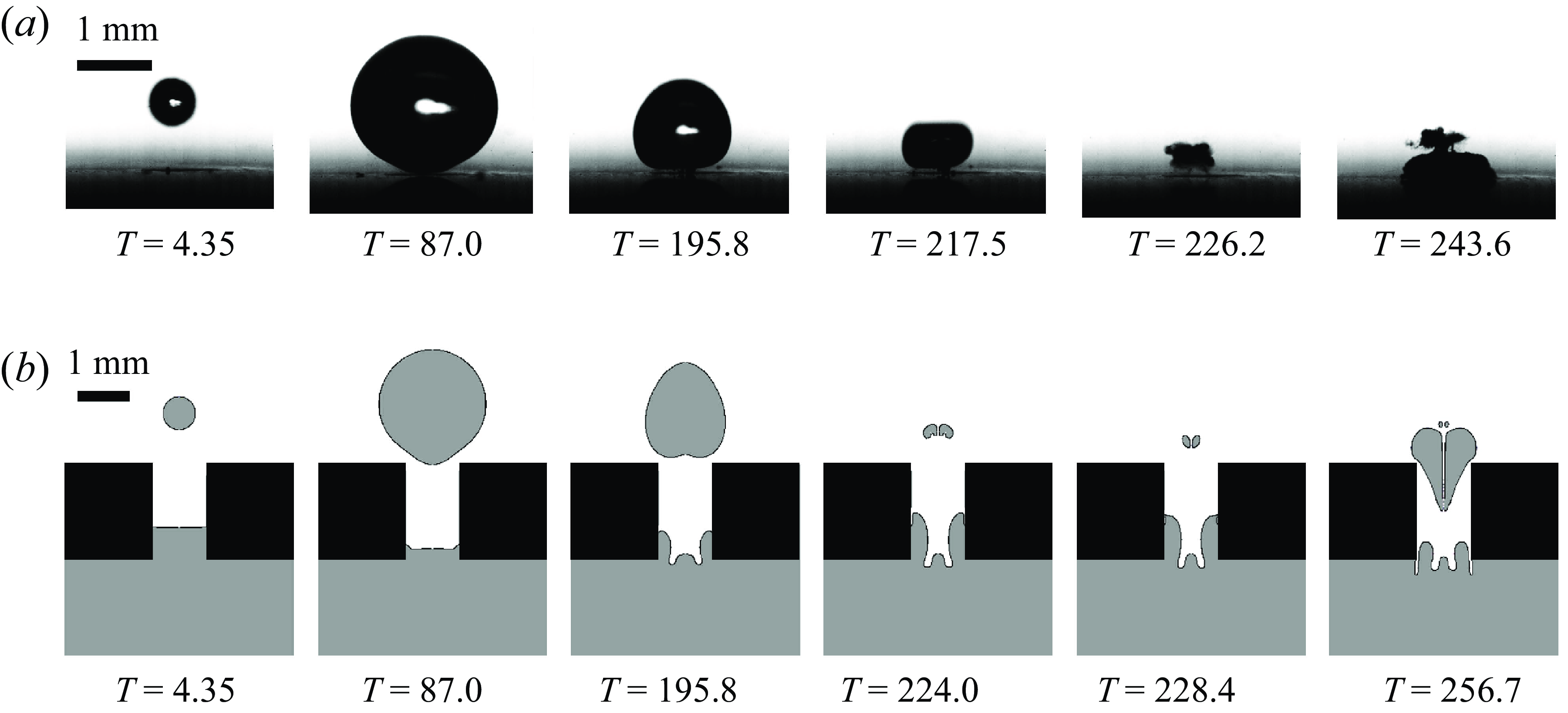
0.11) with (a) selected frames from a high-speed recording (b) showing the simulation results, gas in grey and water in white and black in boundary. Time is stated in microsceonds.

From experiments, it is difficult to observe the gas dynamics in and near the hole. We therefore employ numerical simulations (see Appendix B) to reveal the dynamics obstructed by the cavitation bubble and the boundary. Here, we set up the height
 $h$
of gas–liquid interface as 1.0
 $\rm mm$
and discussed the effect of different heights on bubble dynamics (see Appendix C). The results are shown in figure 8. During expansion, the liquid is pushed into the hole, and an upward jet appears at the bottom of the bubble. The high pressure in the hole causes a small upward jet to be seen at time T = 195.8 μs in the simulations. However, as the bubble moves towards the wall, the presence of the rigid wall causes a downward jet towards to the wall. The re-expanding cavitation bubble due to the reverse pressure gradient pushes again the liquid into the hole. The structure resembles closely the one found in the experiments. While it resembles at first counter-jet it originates from the upper part of the jet of the bubble.
3.1.2. Region 3: neutral collapse
For very small
 $\zeta$
-values,
 $\zeta \lt$
0.001 and
 $\alpha$
 $\approx$
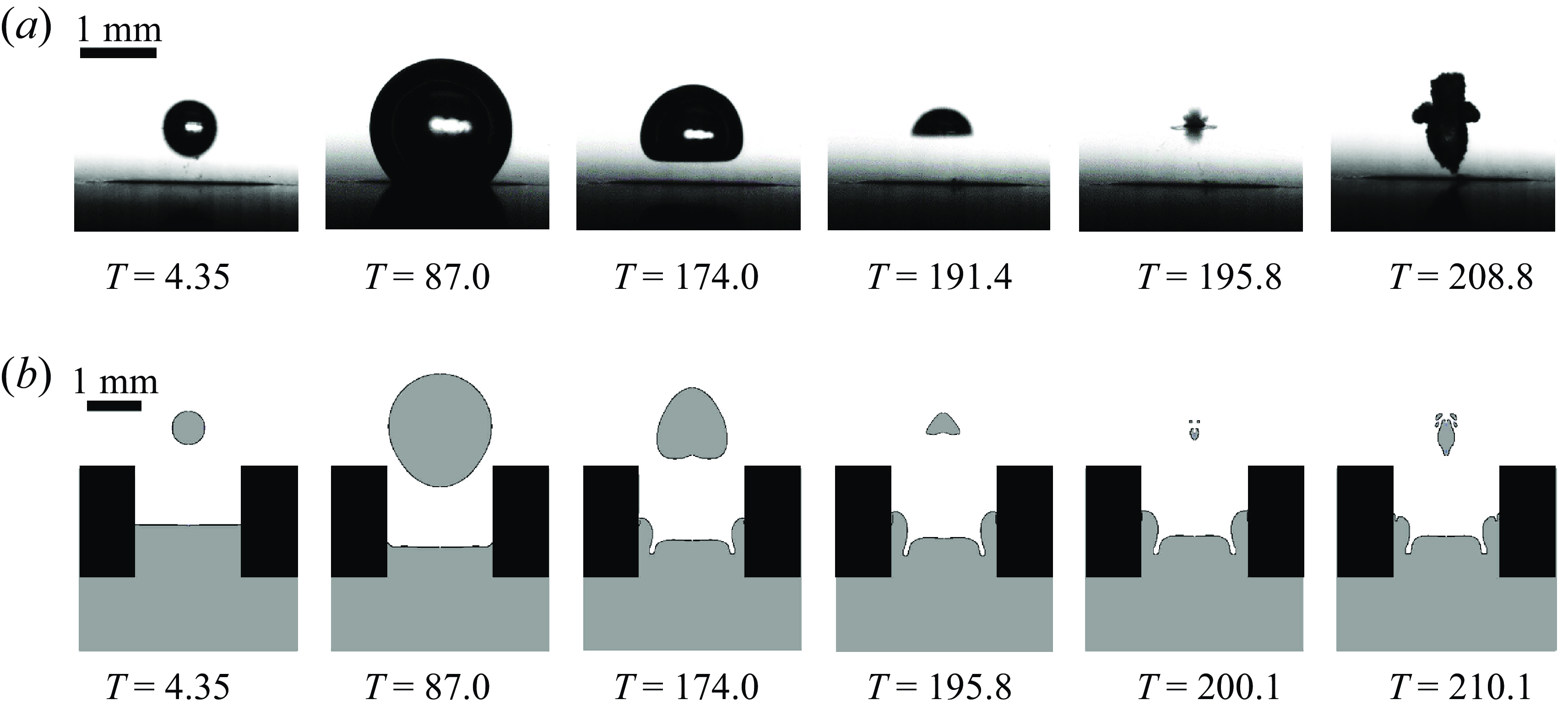
1, the attractive force of the boundary balances the repulsive force of the free surface, resulting in a zero Kelvin impulse. Exemplarily, such a neutral collapse without a centre of mass motion is depicted in figure 9(a) and simulation results in figure 9(b). During shrinkage the bubble develops a wide jet from below, here T = 191.4 μs in the experiment and T = 195.8 μs in the simulation, and causing a flat bottom interface of the bubble. Next, two jets have impacted onto each other during collapse. The second jet has developed later from the top to the bottom, leading to a stagnation point on impact. During rebound, the vapour surrounding the two jets obtains a shape of a vertically aligned hourglass. This kind of collapse has been reported earlier by Zhang et al. (Reference Zhang, Cui, Cui and Wang2015). This is the result from a competition of forces, namely that of the attractive Bjerknes force of the boundary and the opposing buoyancy. The latter was due to the larger size and longer lifetimes of the cavitation bubble. In the present experiments, buoyancy can be ruled out. During bubble collapse, a ring-like toroidal structure appears. We speculate that it is caused by the collapse of the bowl-shaped bubble, see the simulation and experimental frame at T = 174.0 μs. Lindau & Lauterborn (Reference Lindau and Lauterborn2003) has reported this very similar structure when a wide jet in the bubble collides with the sidewall of the collapsing bubble. Here we also have a rather wide jet which for clarity has been recorded from the side and under a
 $45^\circ$
angle to the horizontal, see figure 10. There the frame on the left shows the bubble with the wide jet and on the right the bubble just after collapse. Please note that the views are obtained from separate experiments for the same experimental settings. The side view reveals that the bottom of the upward jet is too wide and overlaps with the sidewall of the bubble that entraps vapour in the shape of a torus. In the subsequent bubble rebound stage, the jet flows towards both sides and the annular structure expands. The toroidal structure can be seen more clearly in the
 $45^\circ$
view.
Neutral bubble collapse of bubble with similar size as the hole and a stand off distance of
 $\gamma$
= 0.75: (a) selected frames from a high-speed recording (b) showing the simulation results.

The bubble collapse observed from two views (
 $\alpha$
 $\approx$
1.0,
 $\gamma$
= 0.75): (a) from the side and (b) under an angle of
 $45^\circ$
to the horizontal.

Next, we focus on the shape of the bubble at collapse for different
 $\gamma$
values, as displayed in figure 11 where the distance to the boundary increases from figure 11(a) to figure 11(e). For small stand-off distance, the toroidal structure during the collapse is pronounced yet fades with increasing stand-off, i.e. it disappears for
 $\gamma$
= 2.0. We explain this observation that the anisotropy parameter
 $\zeta$
decreases with increasing
 $\gamma$
, resulting in a weakening of jet strength and a reduction of the jet width. As a result, the jet collides with the bubble wall later, delaying the formation of the toroidal structure. As
 $\gamma$
increases to 2.0, the jet becomes weaker and fails to form a toroidal structure.
The bubble shape after bubble collapse for
 $\alpha$
 $\approx$
1.0, the toroidal structure disappears increasing
 $\gamma$
-value, times of image recording from (a) to (e) are 174.0, 178.4, 174.0, 182.7 and 200.1 μs.

The bubble shape in different
 $\zeta$
values, (a)
 $\zeta$
 $\approx$
0.02, time (left to right): 204.5, 204.5, 208.9, 204.5 (b)
 $\zeta$
 $\approx$
0.05: 200.1, 204.5, 200.1, 200.1 (c)
 $\zeta$
 $\approx$
0.1: 195.8, 195.8, 191.5, 200.1 (d)
 $\zeta$
 $\approx$
0.15:182.7, 191.5, 191.5, 187.1 μs. Literature data: spark bubble near free surface,
 $R_{\textit{max}}$
= 15
 $\rm mm$
(Xu & Cui Reference Xu and Cui2021) and
 $R_{\textit{max}}$
= 30.26
 $\rm mm$
(Zhang et al. Reference Zhang, Wang and Zhang2016).

3.1.3. Region 4 and region 5: upward jet
Region 4 and region 5 are the regions where the gas-entrapping hole size is larger than the diameter of the bubble at maximum expansion, i.e.
 $\alpha \gt$
1.0. Here we compare the dynamics with the well-studied behaviour of a bubble near a free surface, see for example Zhang et al. (Reference Zhang, Wang and Zhang2016) and Xu & Cui (Reference Xu and Cui2021). The jets can be categorised as strong, intermediate and weak (Supponen Reference Supponen2017). Here, only the cases leading to strong and intermediate jets are discussed. In figure 12, four groups of bubble shapes with approximately equal
 $\zeta$
-values from the regions 4, 5 and the border region are depicted. Each group consists of four representative images captured five frames after the collapse event where the distance between the bubble and the boundary increases from left to right. The rightmost frame depicts the free surface case, while the four frames to the left show bubbles in the presence of holes that increase in diameter from left to right. For
 $\zeta$
 $\approx$
0.15, the bubble’s shape before collapse shows a strong jet, swiftly penetrating the bubble wall due to its high velocity. On the division line when
 $\zeta$
 $\approx$
0.1, the bubble takes on the shape of a triangle after collapse due to the deformation of the interface by the microjet. Compared with
 $\zeta$
 $\approx$
0.15, the microjet is significantly weakened. For the two smaller
 $\zeta$
-values,
 $\zeta$
 $\approx$
0.05 and
 $\zeta$
 $\approx$
0.02, the jet does not penetrate the opposite bubble after the collapse and as
 $\zeta$
decreases, the shape of the bubble is rounder. Figure 13 illustrates the dynamics of the bubble up to the second bubble collapse for
 $\alpha \approx 2.0$
,
 $\gamma =0.56$
,
 $\zeta \approx 0.35$
. Here too, a toroidal bubble collapse is found, that is distinct from the above discussed toroidal collapse in the neutral collapse scenario. A single and strong upward-directed jet is formed already during the early stage of collapse see T = 169.7 μs in figure 13(a) and T = 176.2 μs in figure 13(b) and causing a torus with the jet protruding upwards. It is the result of the bubble shrinkage and the centre of mass motion away from the wall. During the bubble rebound, the toroidal structure expands and merges with the transported and expanding vapour of the jet.
The bubble dynamics in region 5 (
 $\alpha$
 $\approx$
2.0,
 $\gamma$
= 0.56,
 $\zeta$
 $\approx$
0.35): (a) selected frames from a high-speed recording (b) showing the simulation results. The strong jet appears before the bubble collapse, i.e. at T = 169.7μs in (a)
 $T$
= 176.2 μs in (b) and the toroidal structure appears afterwards.

3.2. Analysis of key bubble dynamics parameters
3.2.1. Bubble oscillation periods
The oscillation period of the bubble is typically prolonged in the presence of free surface and shortened near a rigid boundary (Rattray Reference Rattray1951; Shima & Tomita Reference Shima and Tomita1981; Gregorčič et al. Reference Gregorčič, Petkovšek and Možina2007; Reuter et al. Reference Reuter, Zeng and Ohl2022b
). Thus, it is natural to have a look at the prolongation factor
 $k$
which is defined as by
 $T_{c}=k T_{sd}$
, where
 $T_{c}$
is the first oscillation period and
 $T_{sd}$
represents the bubble oscillation period in an unbounded liquid. A compilation of the relationship between the prolongation factor
 $k$
and the anisotropy parameter
 $\zeta$
is summarised in figure 14. It is clear that k cannot be a single-valued function of
 $\zeta$
.
The prolongation factor
 $k$
plotted against the anisotropy parameter
 $\zeta$
. Shima’s theory for a bubble oscillating near a rigid boundary predicts
 $k_p$
, while Gregorčič et al. (Reference Gregorčič, Petkovšek and Možina2007) derived a shortening of the first oscillation by a factor of
 $k_s$
. Here
 $\zeta$
-values refer to (2.5).

Comparing both models with experimental data for the rigid and free boundary confirms both factors,
 $k_s$
and
 $k_p$
, see figure 14. Additionally, we find that small gas-entrapping holes, i.e. for
 $\alpha \lt 1$
, the rigid wall dominates, leading to a prolongation larger than 1 that increases with the asymmetry parameter. Conversely, for large holes,
 $\alpha \gt 1$
, the free surface effect becomes dominant, resulting in a shortened bubble oscillation period. Again
 $k$
increases with the
 $\zeta$
-parameter. Interestingly for
 $\alpha =1$
, the oscillation period of the bubble is basically the same as the oscillation period of the infinite field, indicating that the effects of the rigid wall surface and the free surface on the bubble oscillation period somehow cancel each other.
3.2.2. Bubble displacement
Next, we study the movement of the bubble during the collapse as a function of the anisotropy parameter
 $\zeta$
. We measure the displacement of the bubble from the experiment at minimum bubble volume normalised by the maximum bubble radius,
 $\delta$
=
 $\Delta$
S/
 $R_{\textit{max}}$
. Here
 $\Delta$
S is the distance of the laser focus from the bubble centre at bubble collapse. Figure 15 depicts the
 $\delta$
as a function of
 $\zeta$
. It reveals a power law for non-dimensional displacement
 $\delta$
, with up to the strong jet regime of
 $\zeta \lt 0.1$
. Interestingly, this empirical scaling agrees well with for the experiments reported for the bubble dynamics near a free surface and rigid wall from Supponen (Reference Supponen2017). For the strong jet regime,
 $\zeta \gt 0.1$
, the non-dimensional displacement
 $\delta$
levels off to approximately 0.7.
The bubble centroid displacement
 $\delta$
is plotted as a function of the anisotropy parameter
 $\zeta$
. The symbols are from experiments and the solid line is a fit to a power law resulting to
 $\delta$
= 2.5
 $\zeta ^{0.6}$
. Additionally, the literature data are added from a laser-induced bubble near a rigid wall and a free surface with
 $R_{\textit{max}}$
= 4
 $\rm mm$
, see Supponen (Reference Supponen2017).

4. Conclusions
We conducted a comprehensive study on the dynamics of a cavitation bubble near a gas-entrapping rigid surface. Here, the hole size parameter,
 $0\lt \alpha \lt 2$
, and the distance of the bubble from the surface,
 $0.5\lt \gamma \lt 3.2$
, were varied, resulting in a change of the anisotropy parameter
 $\zeta$
by nearly four orders of magnitude. This anisotropy parameter was derived from a Kelvin impulse model. It accounts for the attraction of the rigid boundary and the repulsion by the gas-entrapping hole. The displacement
 $\delta$
of the bubble scales with this parameter. A second finding is that the rigid wall prolongs the bubble oscillation period, while the free surface shortens it. The oscillation period of the bubble changes significantly with size of the gas-entrapping. Our study also revealed that the different sizes of gas-entrapping holes have a prominent influence on the morphology of the jet, which we divided into three regions: strong jet (
 $0.1\lt \zeta \lt 1$
), intermediate jet (
 $0.001\lt \zeta \lt 0.1$
) and weak jet (
 $0\lt \zeta \lt 0.001$
). While the present study is of fundamental nature, it offers insight into how to control the direction of bubble motion and jetting near complex boundaries. The surface is here not purely passive but may participate in the flow through the transport of gas by active pumping of gas. The gas from the reservoir below the hole could help to restore the liquid–gas interface after a violent collapse but also to dampen the collapse of the main cavitation bubble through the entrainment of non-condensable gas. This ideal behaviour may be achieved by suitable grafted geometries. With these structures, one could test experimentally for a reduction of the erosiveness of cavitation bubble or cavitation cloud collapse on cavitation prone flows. It would be interesting to test gas entrapping structures embedded in boundaries of high-speed flows that show erosion to the boundary. While there are challenges in refilling the cavities with gas, their presence may have an effect on the collapse strength and movement of the cavitation bubbles towards the boundary. Yet, challenges may be the stabilization of the cavities and their refilling with gas. The refilling of the gas entrapping structures is not the only challenge to the idea of reducing cavitation erosion with the added ‘holes’. The presence of the ‘holes’ roughens the surface and could be a source of secondary cavitation or an enhancer of the primary cavitation.
Funding
The financial support from the National Natural Science Foundation of China (nos. 52222904 and 52179092) and the 2115 Talent Development Program of China Agricultural University.
Declaration of interests
The authors report no conflict of interest.
Appendix A. The Kelvin impulse model of a bubble near a gas-entrapping rigid surface
Based on Blake’s expression of the force acting on a bubble in the vertical direction, see (A1), where
 $\Sigma b$
is the area of the semi-infinite boundary,
 $\rho$
is the density of water and
 $\phi$
is the velocity potential of the fluid. According to the cylindrical coordinate system, (A2) is the gradient expression of the cylindrical coordinate system, where the point is (
 $r$
,
 $\theta$
,
 $z$
);
 $r$
is the distance from the projection point of the point on the plane
 $XOY$
to the origin,
 $\theta$
represents the angle between the point projection on the
 $XOY$
plane and the
 $X$
axis,
 $z$
is the distance parallel to the
 $Z$
axis. Here
 \begin{equation} F_S = \rho \int _{\Sigma _b} \left ( \frac {1}{2} (\nabla \phi )^2 \mathbf{n} - \frac {\partial \phi }{\partial n} \nabla \phi \right ) \, {\rm d}S, \end{equation}
 \begin{equation} \nabla \phi = \frac {\partial \phi }{\partial r} \mathbf{e}_r + \frac {1}{r} \frac {\partial \phi }{\partial \theta } \mathbf{e}_{\theta } + \frac {\partial \phi }{\partial z} \mathbf{e}_z. \end{equation}
Equations (A1) and (A2) are combined to obtain the final expression of the force acting on the cavitation bubble, as follows:
 \begin{equation} F_S = \rho \int _{0}^{\infty } r \bigl(u^2 - v^2\bigr) \, {\rm d}r. \end{equation}
In this study, it is assumed that the fluid is an inviscid, incompressible ideal fluid, the pressure and temperature on the surface and inside of the cavitation bubble are uniform and constant and there is no heat and mass transfer on the surface of the cavitation bubble. Also, if the non-spherical disturbance of the cavitation bubble is small enough, the velocity potential of cavitation flow field can be represented by point-source model. It is assumed that if a point source is at
 $r$
= 0,
 $z$
=
 $h$
, only the momentum in the
 $z$
direction is calculated, and the boundary is considered to be at
 $z=0$
. The source strength
 $m$
is the change rate of the volume as follows, where
 $r$
is the bubble radius over time and is the velocity of the bubble:
 \begin{equation} m=4\pi R^2\dot {R}. \end{equation}
Comparison of the angle of the velocity vector between the numerical simulation and analytical model. Here
 $\theta$
is the angle of the velocity vector in clockwise direction;
 $\theta =0$
is along the boundary towards increasing
 $x$
.

According to the principle of mirror method, when the boundary is a gas-entrapping rigid surface, it is simplified into a point source with a strength of
 $m$
and a point sink with a strength of
 $\beta m$
are placed at the position of (0,
 $\lambda$
h), as shown in figure 4. In the source–sink model, it is considered that the point sources and sinks in the lower-half space do not interfere with each other. The ratio of the point source
 $\beta$
and the position
 $\lambda$
is connected with the size of gas-entrapped hole
 $\alpha$
, as shown in (A5) and (A6). For the analytical model, we need to calculate
 $\lambda$
and
 $\beta$
for the intermediate cases, the cases between a free and a rigid boundary. These values are obtained by matching the velocity field of the VoF simulation with that of the potential flow model. This is done by comparing the angle of the velocity vector of both flow fields, i.e.
 $\theta (x)=\tan ^{-1}(u_x/u_y)$
. The parameters
 $\lambda$
and
 $\beta$
are obtained by the best match. A result of this procedure is shown in figure 16 for t = 2 μs. To obtain continuous functions of
 $\lambda$
and
 $\beta$
we, as shown in table 1, utilise monotonic functions, in particular the ’S-curve’ model (Richard’s growth curve model). These curves together with the discrete values from the table are shown in figure 17. Here
 \begin{equation} \lambda =1-e^{-0.83\alpha }, \end{equation}
 \begin{equation} \beta =2-2/(1+(\alpha /1.5)^{2}). \end{equation}
Values of the model parameters: strength sink,
 $\beta$
, and the position factor,
 $\lambda$
.

The strength sink
 $\beta$
and the position factor
 $\lambda$
fit with Richard’s growth curve model. (a) The sink strength
 $\beta$
as a function of the hole size parameter
 $\alpha$
. (b) The position factor
 $\lambda$
as a function of the hole size parameter
 $\alpha$
.

According to the superposition principle of velocity potential at infinite distance, the velocity potential of space flow field can be obtained, as follows, the velocity
 $u$
(A8) in the z direction and the velocity
 $v$
(A9) in the
 $r$
direction can be calculated by using the obtained velocity potential
 $\phi$
:
 \begin{align} \phi \text{=}-\frac {\text{1}}{4\pi }\left [\frac {m}{\sqrt {{{(z-h)}^{2}}+{{(r-0)}^{2}}}}+\frac {m}{\sqrt {{{(z+h)}^{2}}+{{(r-0)}^{2}}}}-\frac {\beta m}{\sqrt {{{(z+\lambda h)}^{2}}+{{(r-0)}^{2}}}} \right ],\nonumber\\ \end{align}
 \begin{equation} u=\frac {\partial \phi }{\partial z}=-\frac {\beta \lambda mh}{4\pi {{({{r}^{2}}+{{\lambda }^{2}}{{h}^{2}})}^{{3}/{2}\;}}}, \end{equation}
 \begin{equation} v=\frac {\partial \phi }{\partial r}=\frac {mr}{2\pi {{({{r}^{2}}+{{h}^{2}})}^{{3}/{2}\;}}}-\frac {\beta mr}{4\pi {{({{r}^{2}}+{{\lambda }^{2}}{{h}^{2}})}^{{3}/{2}\;}}}. \end{equation}
Substituting the obtained velocity
 $u$
and velocity
 $v$
into (A3), the forces acting
 $F_{s}$
on the bubble near gas-entrapping rigid surfaces can be obtained. Among them, this integral is not integrable because it contains
 $\lambda$
, so we make an approximation on it. Here
 \begin{eqnarray} F_s&=&\rho \pi \int _{0}^{\infty }{r}\left ( {{u}^{2}}-{{v}^{2}} \right ){\rm d}r \nonumber\\[5pt] &=&\rho \pi \int _{0}^{\infty }{r}\left [ \frac {{{\left ( \beta \lambda mh \right )}^{2}} - {{\left ( \beta mr \right )}^{2}}}{16{{\pi }^{2}}{{({{r}^{2}}+{{\lambda }^{2}}{{h}^{2}})}^{3}}} \right. \nonumber \\[5pt]&&\left. -\,\left ( \frac {{{\left ( mr \right )}^{2}}}{4{{\pi }^{2}}{{({{r}^{2}}+{{h}^{2}})}^{3}}}-\frac {2\beta {{m}^{2}}{{r}^{2}}}{2\pi {{({{r}^{2}}+{{h}^{2}})}^{{3}/{2}\;}}*4\pi {{({{r}^{2}}+{{\lambda }^{2}}{{h}^{2}})}^{{3}/{2}\;}}} \right ) \right ]{\rm d}r \nonumber \\[5pt] &=&\frac {\rho \pi {{\beta }^{2}}{{m}^{2}}}{16{{\pi }^{2}}}\int _{0}^{\infty }{r}\left [ \frac {{{\lambda }^{2}}{{h}^{2}}-{{r}^{2}}}{{{({{r}^{2}}+{{\lambda }^{2}}{{h}^{2}})}^{3}}}\right ]{\rm d}r-\frac {\rho \pi {{m}^{2}}}{4{{\pi }^{2}}}\int _{0}^{\infty }{r}\left [\frac {{{r}^{2}}}{{{({{r}^{2}}+{{h}^{2}})}^{3}}} \right ]{\rm d}r\nonumber \\[5pt] &&+\,\rho \pi \int _{0}^{\infty }{\frac {2\beta {{m}^{2}}{{r}^{3}}}{2\pi {{({{r}^{2}}+{{h}^{2}})}^{{3}/{2}\;}}*4\pi {{({{r}^{2}}+{{\lambda }^{2}}{{h}^{2}})}^{{3}/{2}\;}}}{\rm d}r} \nonumber \\[5pt] &=&\frac {\rho {{\beta }^{2}}{{m}^{2}}}{16\pi }\int _{0}^{\infty }{\frac {r{{h}^{2}}-{{r}^{3}}}{{{({{r}^{2}}+{{\lambda }^{2}}{{h}^{2}})}^{3}}}}{\rm d}r-\frac {\rho {{m}^{2}}}{4\pi }\int _{0}^{\infty }{r}\left [ \frac {{{r}^{2}}}{{{({{r}^{2}}+{{h}^{2}})}^{3}}} \right ]{\rm d}r\nonumber \\[5pt] &&+\,\frac {\rho \beta {{m}^{2}}}{4\pi }\int _{0}^{\infty }{\frac {{{r}^{3}}}{{{({{r}^{2}}+{{h}^{2}})}^{{3}/{2}\;}}*{{({{r}^{2}}+{{\lambda }^{2}}{{h}^{2}})}^{{3}/{2}\;}}}{\rm d}r} \nonumber \\[5pt] &=&\frac {\rho {{\beta }^{2}}{{m}^{2}}{{\lambda }^{2}}{{h}^{2}}}{16\pi }\int _{0}^{\infty }{\frac {r}{{{({{r}^{2}}+{{\lambda }^{2}}{{h}^{2}})}^{3}}}}{\rm d}r-\frac {\rho {{\beta }^{2}}{{m}^{2}}}{16\pi }\int _{0}^{\infty }{\frac {{{r}^{3}}}{{{({{r}^{2}}+{{\lambda }^{2}}{{h}^{2}})}^{3}}}}{\rm d}r-\frac {\rho {{m}^{2}}}{16\pi {{h}^{2}}}\nonumber \\[5pt] &&+\,\frac {\rho \beta {{m}^{2}}}{4\pi }\int _{0}^{\infty }{\frac {{{r}^{3}}}{{{({{r}^{2}}+{{h}^{2}})}^{{3}/{2}\;}}*{{({{r}^{2}}+{{\lambda }^{2}}{{h}^{2}})}^{{3}/{2}\;}}}{\rm d}r} \nonumber \\[5pt] &=&\frac {\rho {{\beta }^{2}}{{m}^{2}}{{\lambda }^{2}}{{h}^{2}}}{16\pi }*\frac {1}{4{{\lambda }^{4}}{{h}^{4}}}-\frac {\rho {{\beta }^{2}}{{m}^{2}}}{16\pi }*\frac {1}{4{{\lambda }^{2}}{{h}^{2}}}-\frac {\rho {{m}^{2}}}{16\pi {{h}^{2}}}+\frac {\rho \beta {{m}^{2}}}{4\pi {{h}^{2}}{{(\lambda +1)}^{2}}} \nonumber \\[5pt] &=&\frac {\rho {{\beta }^{2}}{{m}^{2}}}{64\pi {{\lambda }^{2}}{{h}^{2}}}-\frac {\rho {{\beta }^{2}}{{m}^{2}}}{64\pi {{\lambda }^{2}}{{h}^{2}}}-\frac {\rho {{m}^{2}}}{16\pi {{h}^{2}}}+\frac {4\rho \beta {{m}^{2}}}{16\pi {{h}^{2}}{{(\lambda +1)}^{2}}} =\frac {(4\beta -{{(\lambda +1)}^{2}})\rho {{m}^{2}}}{16\pi {{h}^{2}}{{(\lambda +1)}^{2}}}. \nonumber\\ \end{eqnarray}
The Kelvin impulse of the bubble can be obtained by integrating the time. Here
 $T_{c}^{Rayleigh}$
is the time when the bubble grows from maximum to minimum. In (2.3), because the integrand
 $m^{2}$
is positive, the positive and negative of the Kelvin impulse
 $I$
is mainly controlled by
 $\beta$
and
 $\lambda$
. If
 $I$
is positive (
 $I\gt 0$
), it means that the bubble will move upward along the positive half-axis of
 $z$
, and if
 $I$
is negative (
 $I\lt 0$
), it will move downward along the negative half-axis of
 $z$
. If
 $I=0$
, the momentum conservation of the bubble and remains stable.
Appendix B. Verification of the simulations
Computational fluid dynamics simulations allow us to gain more knowledge of the flows than what can be observed with the high-speed camera alone. The VoF method based on the OpenFOAM V2006 framework has proven very suitable for the study of cavitation bubbles, particular near various kinds of boundaries, see for example Koch et al. (Reference Koch, Massimini, Boly and Tononi2016), Zeng et al. (Reference Zeng, An and Ohl2022) and Reese et al. (Reference Reese, Schädel, Reuter and Ohl2022). The two-phase solver CompressibleInterFoam accounts for laminar and compressible gases and liquids. Here the liquid is water at a temperature of 20
 $^\circ$
C and an ambient pressure of 1 bar. The explosive expansion of the bubble is initiated with a gas nucleus at time
 $t=0$
, i.e. starting with a compressed bubble of radius
 $R$
(
 $t=0$
) = 9.5
 $\unicode{x03BC} \rm m$
that contains gas at pressure of
 $1.6e^9$
Pa (Plesset Reference Plesset1949; Klaseboer et al. Reference Klaseboer, Hung, Wang, Wang, Khoo, Boyce, Debono and Charlier2005; Li et al. Reference Li, van der Meer, Zhang, Prosperetti and Lohse2020). We ignore mass and heat transport as well as and phase transition, but account for the compressibility of liquid and gas phase. The gas–liquid interface is tracked with the VoF method, and the equations for mass and momentum conservations are used to calculate the fluid flow and fluid–fluid interfaces, respectively,
 \begin{equation} \frac {\partial \rho }{\partial t}+\nabla \cdot (\rho \boldsymbol{u})=0\,\end{equation}
 \begin{equation} \rho \frac {\partial \boldsymbol{u}}{\partial t}+\rho \boldsymbol{u}\cdot \nabla \boldsymbol{u}=-\nabla p+\nabla \cdot \boldsymbol{\tau }+\sigma k\boldsymbol{n}. \end{equation}
Here is the velocity,
 $p$
the pressure, the viscous stress tensor,
 $\sigma$
the coefficient of surface tension, k interfacial curvature, is the unit normal vector of the interface and
 $\rho$
is the density of the fluid. The total density in a computational cell is
 \begin{equation} \rho ={{\alpha }_{1}}{{\rho }_{1}}+{{\alpha }_{2}}{{\rho }_{2}}\ \end{equation}
where
 $\rho _{1}$
and
 $\rho _{2}$
are the densities of water and air, respectively, and
 $\alpha _{1}$
and
 $\alpha _{2}$
are the respective volume fractions, such that
 $\alpha _{1} + \alpha _{2}=1$
.
Here, the finite volume method is applied to discretise the conservation of momentum and mass, and the PIMPLE algorithm is utilised to solve for pressure and velocity. Given that the convection term is zero in pure air or water, the advection equation, used to capture the gas–liquid interface, can be expressed by the volume fraction of a phase. At this point, the volume fraction of this phase ranges between 0 and 1, allowing the equation to be represented as
 \begin{equation} \frac {\partial }{\partial t}({{\alpha }_{1}})+\boldsymbol{u}\nabla \cdot {{\alpha }_{1}}+\nabla \cdot [{{\boldsymbol{u}}_{\alpha }}{{\alpha }_{1}}{{\alpha }_{2}}]=0. \end{equation}
It is evident from (B4) that the third term is zero, and having a non-zero value only at the gas–liquid interface. The compressible velocity direction in the additional term in the formula should be perpendicular to the gas–liquid interface to nullify its impact on the flow field, ensuring the convergence of the velocity field and the compression effect. The compression speed set through the following expression:
 \begin{equation} u_{\alpha }=\min ({C}_{\alpha }|\boldsymbol{u}|,\max (|\boldsymbol{u}|))\frac {\nabla \alpha }{|\nabla \alpha |}. \end{equation}
Here
 $ u_{\alpha }$
is the compressibility coefficient of the interface. The Tait equation for vapour is incorporated as
 \begin{equation} \rho _{w}={\rho }_{v}{\left(\frac {p+B}{{{p}_{v}}+B}\right)}^{k}. \end{equation}
Here,
 ${\rho }_{v}$
and
 ${p}_{v}$
represent reference density and pressure, respectively,
 ${\rho }_{w}$
is water density and standard atmospheric pressure
 $p$
. Here B is a constant with a value of 306MPa, and k is equal to 7.15.
(a) Sketch for the computational region (
 $10 \times 28\,\rm mm$
). Blue represents water, grey gas, and white the rigid boundary. (b) Zoomed in region, where the inner part has a cell with of
 $1.25\mu$
. (c) Details of the mesh of the bubble.

(a) Microscopic image of the gas entrapping hole. (b) The height of interface
 $h$
is from the rigid wall to the topper of interface.

The simulation model and the boundary conditions are provided in figure 18. In the experiments we know that the liquid–gas interface is not flush with the front surface but reclined into the hole. We estimate this depth to be approximately
 $1\,$
mm. This value is used in all VoF simulations used in the paper. For this simulation,
 $2-3 \times 10^6$
computational grids are used to solve the respective governing equations assigned to each computational unit. The solver solves for the pressure p, velocity u and the phase fraction field
 $\alpha _1$
and
 $\alpha _2$
.
(a) Comparison of three different thicknesses
 $D$
of the rigid wall having the same non-dimensional hole size
 $\alpha$
 $\approx$
0.5 and constant height
 $h$
. (b) Only the interface depth
 $h$
is varied. revealing a significant effect on the bubble dynamics. Here
 $\gamma =1$
for all cases.

Appendix C. The position of gas–liquid interface
We checked the shape of the hole with a confocal microscope, see figure 19(a). The shape is round without bevelling or chamfering. When the hole is submerged, it first forms a flat interface pinned at the sides. Upon deeper immersion, this interface is pushed by the hydrostatic pressure deeper into the hole. We now account in the VoF simulations for a gas–liquid interface being not flush with the rigid boundary but at a depth
 $h$
(Figure19
b) within the hole. In the experiments we know that the liquid–gas interface is not flush with the front surface but reclined into the hole. We estimate this depth to be approximately
 $1\,$
mm. This value is used in all VoF simulations used in the manuscript. Next, we include the effect of an interface position within hole. Figure 20 demonstrates the effect of the interface position and depth of the hole. In figure 20(a) the gas–liquid interface height
 $h$
remains constant while the thickness
 $D$
varies. As expected, there is little effect on the bubble dynamics. In figure 20(b) only
 $h$
changes and the wall thickness
 $D$
remains constant. We find a rather strong effect on the position of the interface. The shorter lifetime for smaller
 $h$
can be explained that the bubble is surrounded by less mass, and therefore it takes less time to displace it, i.e. the bubble ‘sees’ a lower inertia.
Three simulation cases with constant boundary thickness
 $D=2\,$
mm and position of the interface below the rigid boundary in (a)
 $h=1.5\,$
mm, (b)
 $h=1.0\,$
mm and (c)
 $h=0.5\,$
mm. White represents water, grey gas and black the boundary. The time is stated in microseconds.

Besides the obvious reduction of the lifetime, we also find an effect on the non-spherical bubble dynamics, see figure 21. While the thickness of the orifice is not affecting bubble dynamics, the position of the interface matters. Therefore, we present a few snapshots from simulations where the interface position is varied from
 $h=1.5\,$
mm to
 $h=0.5\,$
mm with a constant thickness of
 $D=2\,$
mm, see figure 21. The simulation results are shown in figure 21. Consistently, we find for all
 $h$
that the liquid is pushed into the hole during the early expansion
 $T=4.35\,\unicode{x03BC}$
s. For
 $h=1.5\,$
mm (figure 21
a) during the bubble shrinkage, an upward jet does not appear at the bottom of the bubble, see
 $T=195.8\,\unicode{x03BC}$
s. But for
 $h=1.0\,$
mm (figure 21
b) and 0.5 mm (figure 21
c), the upward jet will is developed, as
 $h$
increases, see
 $T=195.8\,\unicode{x03BC}$
s. Also, during the bubble collapse, the distance that the bubble migrates downward increases as the height of the interface
 $h$
increases. We find that the bubble dynamics is affected by the filling of the hole, yet in the parameter range studied the direction of bubble migration and the direction of the microjet remains.