1. Introduction
The spreading of Newtonian drops impacting on solid surfaces (Worthington Reference Worthington1883; Roisman et al. Reference Roisman, Prunet-Foch, Tropea and Vignes-Adler2002; Clanet et al. Reference Clanet, Béguin, Rhichard and Quéré2004; Lee et al. Reference Lee, Laan, de Bruin, Skantzaris, Shahidzadeh, Derome, Carmeliet and Bonn2015) has received significant attention in the literature, being the subject of many review articles (Rein Reference Rein1993; Yarin Reference Yarin2006; Josserand & Thoroddsen Reference Josserand and Thoroddsen2016). Variants of this problem have been explored as well, such as the impact of non-Newtonian drops (Crooks & Boger Reference Crooks and Boger2000; Cooper-White, Crooks & Boger Reference Cooper-White, Crooks and Boger2002; Luu & Forterre Reference Luu and Forterre2009, Reference Luu and Forterre2014; Boyer et al. Reference Boyer, Sandoval-Nava, Snoeijer, Dijksman and Lohse2016; Oishi, Thompson & Martins Reference Oishi, Thompson and Martins2019; Isukwem et al. Reference Isukwem, Godefroid, Monteux, Bouttes, Castellani, Hachem, Valette and Pereira2024b,Reference Isukwem, Nemer, Hachem and Pereirac), the drop impact onto inclined planes (Laan et al. Reference Laan, de Bruin, Bartolo, Josserand and Bonn2014; LeClear et al. Reference LeClear, LeClear, Abhijeet, Park and Choi2016), onto a target (Arora, Ligoure & Ramos Reference Arora, Ligoure and Ramos2016; Arora et al. Reference Arora, Louhichi, Vlassopoulos, Ligoure and Ramos2021), onto a permeable body or a mesh (Lorenceau & Quéré Reference Lorenceau and Quéré2003; Soto et al. Reference Soto, Girard, Le Helloco, Binder, Quéré and Varanasi2018; Su et al. Reference Su, Luo, Chu, Cai, Le, Zhang and Chen2020), the drop impact on a thin horizontal fibre (Lorenceau, Clanet & Quéré Reference Lorenceau, Clanet and Quéré2004; Comtet, Keshavarz & Bush Reference Comtet, Keshavarz and Bush2016), on a liquid film (Blackwell et al. Reference Blackwell, Deetjen, Gaudio and Ewoldt2015; Guo & Lian Reference Guo and Lian2018), and the drop–drop collision (Ramírez-Soto et al. Reference Ramírez-Soto, Sanjay, Lohse, Pham and Vollmer2020). These flow configurations are intrinsically associated with multiple applied processes, including forensic science, atomization, spray coating, firefighting, inkjet printing, and more recently three-dimensional (3-D) printing of electronic components, organs, tissues and prosthetics (Bordoloi & Longmire Reference Bordoloi and Longmire2014; Laan et al. Reference Laan, de Bruin, Bartolo, Josserand and Bonn2014; Murphy & Atala Reference Murphy and Atala2014; Ryu et al. Reference Ryu, Sen, Nam and Lee2017; Kumar et al. Reference Kumar, Tripathy, Nam, Lee and Sen2018; Vijayavenkataraman et al. Reference Vijayavenkataraman, Yan, Lu, Wang and Fuh2018; Modak et al. Reference Modak, Kumar, Tripathy and Sen2020).
In the mentioned applications, the control of the drop-spreading dynamics emerges from a delicate balance between inertial, interfacial and viscous stresses. Furthermore, the drop expansion is also affected by interactions between the impacting object and the impacted substrate (Quéré Reference Quéré2008; Bonn et al. Reference Bonn, Eggers, Indekeu, Meunier and Rolley2009; Duez et al. Reference Duez, Ybert, Clanet and Bocquet2010; Carlson, Do-Quang & Amberg Reference Carlson, Do-Quang and Amberg2011; Josserand & Thoroddsen Reference Josserand and Thoroddsen2016), and it is strongly facilitated by the use of repellent surfaces, such as superhydrophobic ones (Richard, Clanet & Quéré Reference Richard, Clanet and Quéré2002; Clanet et al. Reference Clanet, Béguin, Rhichard and Quéré2004; Josserand & Thoroddsen Reference Josserand and Thoroddsen2016; Quetzeri-Santiago et al. Reference Quetzeri-Santiago, Yokoi, Castrejon-Pita and Castrejon-Pita2019), and plates heated above the Leidenfrost temperature (Leidenfrost Reference Leidenfrost1756; Garmett Reference Garmett1878; Biance, Clanet & Quéré Reference Biance, Clanet and Quéré2003; Lee et al. Reference Lee, Harth, Rump, Kim, Lohse, Fezzaa and Je2020; Graeber et al. Reference Graeber, Regulagadda, Hodel, Kuttel, Landolf, Schutzius and Poulikakos2021; Wang et al. Reference Wang, Fei, Lei, Wang and Luo2022). In this connection, an essential and scarcely explored flow scenario regards the impact of a drop onto a solid surface in inverse Leidenfrost conditions (Hall et al. Reference Hall, Board, Clare, Duffey, Playle and Poole1969; Adda-Bedia et al. Reference Adda-Bedia, Kumar, Lechenault, Moulinet, Schillaci and Vella2016; Gauthier et al. Reference Gauthier, Diddens, Proville, Lohse and van der Meer2019), i.e. the solid surface is covered with a thin layer of liquid nitrogen that partially evaporates as the drop expands after its impact. The generated vapour film prevents the drop's contact with both the liquid nitrogen and the solid plate, favouring the spread of the impacting object. In such a scenario, the levitating drop would experience a biaxial extensional deformation, a point discussed in very few works in the literature (Arora et al. Reference Arora, Fromental, Mora, Phou, Ramos and Ligoure2018; Louhichi et al. Reference Louhichi, Charles, Phou, Vlassopoulos, Ramos and Ligoure2020; Charles et al. Reference Charles, Louhichi, Ramos and Ligoure2021) that deserves deeper investigations. Attempts to extend the existing analyses should then naturally contemplate the physical mechanisms governing the drop spreading for a wide range of viscosity, surface tension, density and impact velocity.
In the present work, we investigate the spreading of falling ambient-temperature Newtonian drops, after their normal impact on a solid plate covered with a thin layer of liquid nitrogen. Due to the temperature difference between a drop and the liquid nitrogen, the latter partially evaporates, generating a vapour film that maintains the drop in levitation as it expands. This is the inverse Leidenfrost effect. We extend previous studies on this phenomenon by highlighting the physical mechanisms driving the spreading of the levitating drops after their impact. Three spreading regimes are observed: (i) inertio-capillary (balancing inertial and capillary stresses); (ii) inertio-viscous (balancing inertial and viscous stresses); and (iii) inertio-viscous-capillary (for which inertia, capillarity and viscosity are all relevant). These regimes are underlined through a mixed approach combining experiments and 3-D numerical simulations based on an adaptive variational multi-scale method for two fluids (the drop and the surrounding nitrogen vapour). Experimental and numerical results are explored in light of spreading dynamics analyses, energy transfer, and scaling laws for the drops’ maximum diameter and spreading time.
The organization of the paper is as follows. A detailed description of the physical formulation and the mixed experimental–numerical method is presented in § 2. Experimental and numerical results are discussed in § 3. Finally, conclusions and perspectives are drawn § 4.
2. Problem statement, mixed experimental–numerical approach, and relevant dimensionless parameters
2.1. Problem statement
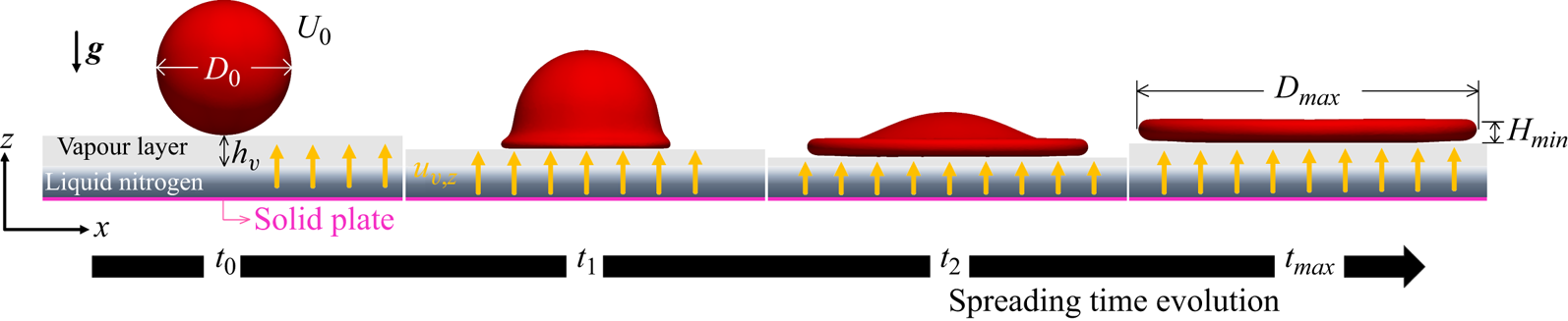
As illustrated in figure 1, we consider the spreading time evolution of an ambient-temperature Newtonian falling drop (in red) of initial diameter  $D_0$, density
 $\rho$, and viscosity
 $\eta$, after it impacts at the instant
 $t_0$ with velocity
 $U_0$ a solid plate (in magenta) covered with a thin layer of liquid nitrogen (in dark blue) at temperature
 $T_l$. As the drop expands, liquid nitrogen evaporates, generating a vapour film (in grey) of thickness
 $h_v$, density
 $\rho _v$, viscosity
 $\eta _v$, and normal velocity
 $u_{v,z}$ that maintains the drop in levitation. Consequently, the latter spreads in inverse Leidenfrost conditions until achieving its maximum diameter
 $D_{max}$ and minimal thickness
 $H_{min}$ at the instant
 $t_{max}$. Surface tension between the drop and the surrounding gases is denoted by
 $\sigma$.
An ambient-temperature Newtonian drop (in red) of initial diameter  $D_0$, density
 $\rho$, and viscosity
 $\eta$ falls by gravity
 $g$ and impacts at the instant
 $t_0$ with velocity
 $U_0$ a solid plate (in magenta) covered with a thin layer of liquid nitrogen (in dark blue) at temperature
 $T_l$. As the drop expands, liquid nitrogen evaporates, generating a vapour film (in grey) of thickness
 $h_v$, density
 $\rho _v$, viscosity
 $\eta _v$, and normal velocity
 $u_{v,z}$ that maintains the drop in levitation. Hence the latter spreads in inverse Leidenfrost conditions until achieving its maximum diameter
 $D_{max}$ and minimal thickness
 $H_{min}$ at the instant
 $t_{max}$.

The dynamics regarding the eventual retraction of the drop induced by surface tension effects is out of the scope of the present work. Splashing events are not taken into account either. More specifically, for some of our experiments, we do observe azimuthal instabilities and splashing, which are typically favoured by high impact velocities, low drop viscosities, and low surface tensions. These instabilities are equally captured by our numerical simulations. Nevertheless, their development will be a matter of future works. Hence results involving splashing events were excluded from the data presented in § 3.
2.2. Mixed experimental–numerical approach
As schematized in figure 2(a), the impact and spreading events are experimentally recorded simultaneously by two high-speed cameras: (1) from the top by a Phantom V 7 : 3 operated at  $6700\ {\rm fps}$ with resolution
 $800 \times 600\ {\rm pixels}^2$, where the angle between the camera axis and the vertical plane is approximately
 $10^{\circ }$); and (2) from the side by a Phantom Miro M310 operated at
 $3200\ {\rm fps}$ with resolution
 $1280 \times 800\ {\rm pixels}^2$. An LED backlight system provides the necessary lighting level. The millimetric drop of temperature
 $T_0$ varying between
 $18.5\,^{\circ }{\rm C}$ and
 $22.5\,^{\circ }{\rm C}$ falls by gravity from a nozzle and hits a solid quartz plate (in magenta) covered with a thin liquid nitrogen layer (in blue) at temperature
 $T_l = - 196\,^{\circ }{\rm C}$, which partially evaporates. (Details on the experimental set-up are given in Arora et al. Reference Arora, Fromental, Mora, Phou, Ramos and Ligoure2018.) Due to the temperature difference
 $\Delta T$ between the drop and the liquid nitrogen, heat diffuses through the vapour phase, vaporizing part of the liquid nitrogen. The escaping vapour (in grey) of normal velocity
 $u_{v,z}$ is then confined below the drop within a thin film of thickness
 $h_v$, and lubrication generates an overpressure that sustains the drop in levitation during its spreading (values of
 $h_v$ and
 $u_{v,z}$ are detailed at the end of this subsection). Typical snapshots captured by the top-view and side-view cameras are shown in figures 2(b) and 2(c), respectively. The time evolution of the sheet size is measured with ImageJ software by analysing top-view images. We first subtract the background image from the expansion movie and highlight the rim by binary thresholding. This allows us to determine the sheet's contour and measure its area
 $A$ as a function of time. An apparent instantaneous sheet's diameter is simply deduced as
 $D = \sqrt {4A/{\rm \pi} }$.
(a) Schematic illustration of the experimental set-up for the investigation of the impacting drops in an inverse Leidenfrost situation. The millimetric drop falls by gravity from a nozzle and hits a solid quartz plate (in magenta) covered with a thin layer of liquid nitrogen (in blue), which partially evaporates, generating a vapour film (in grey) that maintains the drop in levitation during its spreading. The impact events are experimentally recorded simultaneously by two high-speed cameras: (1) from the top; and (2) from the side. Typical snapshots captured by the top-view and the side-view cameras are shown in (b,c), respectively.

Initial drop diameters  $D_0$ are in the range 3.5–5 mm, and the experimental impact velocity
 $U_0$ varies from
 $3\ {\rm m}\ {\rm s}^{-1}$ to
 $4.25\ {\rm m}\ {\rm s}^{-1}$. Glycerol–water mixtures (
 $1050 \leqslant \rho \leqslant 1260\ {\rm kg}\ {\rm m}^{-3}$,
 $0.00105 \leqslant \eta \leqslant 1.91\ {\rm Pa}\ {\rm s}$,
 $\sigma = 68\ {\rm mN}\ {\rm m}^{-1}$) and silicone oils (
 $913 \leqslant \rho \leqslant 970\ {\rm kg}\ {\rm m}^{-3}$,
 $0.0052 \leqslant \eta \leqslant 5\ {\rm Pa}\ {\rm s}$,
 $\sigma = 20\ {\rm mN}\ {\rm m}^{-1}$) are used.
Our computational approach is based on a general solver (CIMLIB-CFD, a parallel, finite-element library; Coupez & Hachem Reference Coupez and Hachem2013) that takes into account the rheological behaviour of two fluid phases (the drop and the nitrogen vapour; the liquid nitrogen phase is not considered here), as well as surface tension effects (Riber et al. Reference Riber, Valette, Mesri and Hachem2016; Pereira et al. Reference Pereira, Larcher, Hachem and Valette2019; Valette et al. Reference Valette, Hachem, Khalloufi, Pereira, Mackley and Butler2019, Reference Valette, Pereira, Riber, Sardo, Larcher and Hachem2021; Pereira, Hachem & Valette Reference Pereira, Hachem and Valette2020; Isukwem, Hachem & Pereira Reference Isukwem, Hachem and Pereira2024a; Isukwem et al. Reference Isukwem, Godefroid, Monteux, Bouttes, Castellani, Hachem, Valette and Pereira2024b,Reference Isukwem, Nemer, Hachem and Pereirac). More precisely, the momentum equation applied to the considered solenoidal flows ( $\boldsymbol {\nabla } \boldsymbol {\cdot }\boldsymbol {u} = 0$) reads
 \begin{equation} \rho \left( \frac{\partial \boldsymbol{u}}{\partial t} + \boldsymbol{u} \boldsymbol{\cdot}\boldsymbol{\nabla} \boldsymbol{u} - \boldsymbol{g} \right) ={-} \boldsymbol{\nabla} p + \boldsymbol{\nabla}\boldsymbol{\cdot} \boldsymbol{\tau} + \boldsymbol{f}_{st} , \end{equation}
in which  $\boldsymbol {u}$,
 $p$,
 $\boldsymbol {\tau }$,
 $\boldsymbol {\nabla }$,
 $\boldsymbol {g}$,
 $\boldsymbol {\nabla } \boldsymbol {\cdot }$ and
 $\boldsymbol {f}_{st}$ are, respectively, the velocity vector
 $\boldsymbol {u} = \lbrace u_x, u_y, u_z \rbrace$, the pressure, the extra-stress tensor, the gradient operator, the gravity vector, the divergence operator, and a capillary term related to the surface tension force. The latter is defined as
 $\boldsymbol {f}_{st} = -\sigma \kappa \varPhi \boldsymbol {n}$, where
 $\sigma$,
 $\kappa$,
 $\varPhi$ and
 $\boldsymbol {n}$ are the drop surface tension with the surrounding gas, the curvature of the drop–gas interface, the Dirac function locating the liquid–gas interface, and its normal vector, respectively. In addition, the extra-stress tensor is given by
 $\boldsymbol {\tau } = \eta \dot {\boldsymbol {\gamma }}$, in which
 $\dot {\boldsymbol {\gamma }}$ represents the rate-of-strain tensor defined as
 $\dot {\boldsymbol {\gamma }} = \boldsymbol {\nabla }\boldsymbol {u} + \boldsymbol {\nabla } \boldsymbol {u}^{\rm T}$. The norm of
 $\dot {\boldsymbol {\gamma }}$ is called the deformation rate, being defined as
 $\| \dot {\boldsymbol {\gamma }}\| = ( \frac {1}{2} \dot {\boldsymbol {\gamma }}: \dot {\boldsymbol {\gamma }} ) ^{{1}/{2}}$. Our numerical methods are based on a variational multi-scale approach combined with anisotropic mesh adaptation with highly stretched elements (Riber et al. Reference Riber, Valette, Mesri and Hachem2016; Pereira et al. Reference Pereira, Larcher, Hachem and Valette2019, Reference Pereira, Hachem and Valette2020; Valette et al. Reference Valette, Hachem, Khalloufi, Pereira, Mackley and Butler2019, Reference Valette, Pereira, Riber, Sardo, Larcher and Hachem2021; Isukwem et al. Reference Isukwem, Hachem and Pereira2024a,Reference Isukwem, Godefroid, Monteux, Bouttes, Castellani, Hachem, Valette and Pereirab,Reference Isukwem, Nemer, Hachem and Pereirac). The time evolution of the drop–gas interface is captured using a level-set function (Hachem et al. Reference Hachem, Khalloufi, Bruchon, Valette and Mesri2016). Fluid properties are interpolated through the level-set function whose value varies from positive within the drop to negative in the vapour (and zero at the interfaces between the different fluid phases). Supplemental details concerning the interface capturing and the level-set function are available in Appendix A.
The 3-D numerical configuration taken into account is illustrated in figure 3. Four numerical snapshots show the spreading time evolution. Only the drop (in red) and the vapour phase (in blue) are considered. The mesh (composed of approximately  $10^6$ elements; see black lines on the right-hand side of the second and third snapshots) is adapted around each interface. The corresponding zero isovalues for the level-set function are also shown (in red). The considered numerical drops are millimetric,
 $3 \leqslant D_0 \leqslant 10\ {\rm mm}$. Furthermore, wide ranges of liquid properties are explored numerically:
 $250 \leqslant \rho \leqslant 2500\ {\rm kg}\ {\rm m}^{-3}$,
 $0.001 \leqslant \eta \leqslant 10\ {\rm Pa}\ {\rm s}$,
 $0.005 \leqslant \sigma \leqslant 1\ {\rm N}\ {\rm m}^{-1}$. The numerical impact velocity varies from
 $1\ {\rm m}\ {\rm s}^{-1}$ to
 $5\ {\rm m}\ {\rm s}^{-1}$. Concerning the nitrogen vapour phase (in blue), both viscosity
 $\eta _{v}$ and density
 $\rho _{v}$ are constant at respectively
 $1.74 \times 10^{-5}\ {\rm Pa}\ {\rm s}$ and
 $1.25\ {\rm kg}\ {\rm m}^{-3}$. Initial and boundary conditions for the flow equations are: initial vertical impact velocity
 $U_0$ within the drop;
 $\boldsymbol {u}_v = \lbrace 0, 0, u_{v,z} \rbrace$ for the vapour phase at the bottom wall (normal inlet velocity represented by yellow arrows in figure 3); and zero normal stress in the other walls of the domain.
Numerical configuration taken into account. The drop (in red) of diameter  $D_0$ falls by gravity
 $\boldsymbol {g}$ and reaches the velocity
 $U_0$ at
 $t_0$, after which it expands in levitation induced by the action of a vapour (in blue) counter-flow whose inlet vertical velocity
 $u_{v,z}$ is imposed at the bottom wall of the computational domain (yellow arrows). At the instant
 $t_{max}$, the drop achieves its maximum diameter
 $D_{max}$ and a minimum height
 $H_{min}$. The spreading time evolution is represented by four snapshots. The used mesh (composed of approximately
 $10^6$ elements) adapted around each interface (drop in red and vapour in blue) is illustrated by the black lines in the second and third snapshots.

The normal velocity of the nitrogen vapour  $u_{v,z}$ imposed as a boundary condition at the bottom wall (yellow arrows in figure 3) is calculated by assuming that the energy related to vaporization is brought by the thermal conduction through the vapour film induced by the temperature difference between the drop and the liquid nitrogen:
 \begin{equation} L_v\,\frac{{\rm d}m_v}{{\rm d}t} \sim K_v D^2\,\frac{\Delta T}{h_v} , \end{equation}
in which  $L_v$ is the nitrogen latent heat of vaporization,
 ${\rm d}m_v/{\rm d}t$ is the rate of evaporation (mass per unit time),
 $K_v$ is the thermal conductivity of vapour, and
 $D$ is the instantaneous diameter of the drop. Since
 ${\rm d}m_v/{\rm d}t \sim \rho _v D^2 u_{v,z}$, the normal inlet velocity of the nitrogen vapour reads
 \begin{equation} u_{v,z} \sim \frac{K_v}{\rho_v L_v}\,\frac{\Delta T}{h_v} . \end{equation}
This equation is imposed as the normal inlet velocity of the nitrogen vapour at the bottom wall, with  $h_v$ being defined numerically as the smallest distance between the drop and the bottom wall at each time step (hence
 $u_{v,z}$ increases as the drop moves downwards, diminishing
 ${h_v}$).
The size of the smallest mesh elements in our numerical domain is taken as ten times smaller than the minimum  ${h_v}$ reached during the drop-spreading process
 ${h_{v,min}}$. Such a value is estimated by using lubrication theory. More specifically, the pressure variation within the vapour film given by the lubrication theory
 $\Delta p \sim \eta _v ({u_{v,z}}/{h_v})({D^2}/{h_v^2})$ (Gauthier et al. Reference Gauthier, Diddens, Proville, Lohse and van der Meer2019) is compared to the drop inertial stress at the impact
 ${\sim }\rho U_0^2$, leading to
 \begin{equation} u_{v,z} \sim \frac{\rho U_0^2 h_v}{\eta_v}\,\frac{h_v^2}{D^2} . \end{equation}
By combining (2.3) and (2.4), and taking  $D = D_0$, we deduce an expression for
 $h_{v, min}$ as
 \begin{equation} h_{v, min} \sim \left( \frac{K_v \eta_v}{\rho_v L_v}\,\frac{D_0^2}{\rho U_0^2}\,\Delta T \right)^{1/4} , \end{equation}
leading to  $h_{v,min} \sim {O} ( 10^{1} )\ \mathrm {\mu }{\rm m}$ (with
 $L_v = 2 \times 10^5\ {\rm J}\ {\rm kg}^{-1}$,
 $K_v = 0.026\ {\rm W}\ {\rm mK}^{-1}$,
 $\rho _v = 1.25\ {\rm kg}\ {\rm m}^{-3}$,
 $\eta _v = 1.74 \times 10^{-5}\ {\rm Pa}\ {\rm s}$), values of the same order of magnitude as those reported by Biance et al. (Reference Biance, Clanet and Quéré2003) and Gauthier et al. (Reference Gauthier, Diddens, Proville, Lohse and van der Meer2019) under static levitation conditions. Hence a minimal mesh size
 $\varDelta _{min}$ of
 $1\ \mathrm {\mu }{\rm m}$ is chosen (it is important to underline that this choice of
 $\varDelta _{min}$ is also based on the supplemental numerical analyses presented in Appendix A).
For the impact events considered experimentally here, the drop reaches its maximum diameter  $D_{max}$ less than 10 ms after the beginning of the spreading process (
 $t_{max} < 10$ ms). In such a time interval, the heat exchange between the drop the nitrogen vapour is given by
 \begin{equation} {-}\rho D_0^3 c_p\,\frac{{\rm d}T}{{\rm d}t} \sim K_v D^2\,\frac{ T - T_l }{h_v} , \end{equation}
where  $c_p$ is the specific heat of the drop, and
 $T$ is its instantaneous temperature. Consequently,
 \begin{equation} T \sim \left( T_0 - T_l \right) \exp \left( \frac{-K_v D^2 t}{\rho D_0^3 c_p h_v} \right) + T_l . \end{equation}
We find thus that the temperature of the drop at  $t < 10$ ms is approximately equal to
 $T_0$ (with
 $c_p = 4181\ {\rm J}\ {\rm kg}^{-1}\ {\rm K}^{-1}$,
 $h_v = 10\ \mathrm {\mu }{\rm m}$ and
 $D < 6D_0$). For this reason, in our numerical simulations, the drop properties are considered constant throughout the spreading process.
Finally, note that liquid nitrogen and phase changes are not considered in our numerical framework. The expansion of the levitating drops in inverse Leidenfrost conditions is described exclusively through gravitational, inertial, capillary and viscous parameters related to the interactions between the drop and the nitrogen vapour. Nevertheless, we will show that such physical ingredients are sufficient to capture the main features observed in our experiments.
2.3. Relevant dimensionless numbers
The important dimensionless quantities of the problem can be stressed by a classical dimensional analysis based on the Buckingham  $\varPi$ theorem with the physical system defined in terms of six physical variables (
 $D_0$,
 $U_0$,
 $g$,
 $\rho$,
 $\eta$,
 $\sigma$) that may be expressed in terms of three fundamental units, i.e. mass, length and time. The Buckingham
 $\varPi$ theorem thus indicates that the system may be uniquely described in terms of three dimensionless groups:
 \begin{equation} {Fr} = \frac{\rho g D_0}{\rho U_0^2}, \quad {Re} = \frac{\rho U_0^2}{\eta (U_0/D_0)}, \quad {We} = \frac{\rho U_0^2}{\sigma/D_0} , \end{equation}
where  ${Fr}$ is the Froude number,
 ${Re}$ is the Reynolds number, and
 ${We}$ is the Weber number. Since we consider here millimetric drops for which
 $\eta$ and/or
 $\sigma$ are relatively high,
 $\rho g D_0$ ends up playing a marginal role in comparison to the other stress terms, i.e.
 ${Fr} \leqslant 0.01$ (this will be shown in detail in the next section). Hence the particular flow scenarios explored here can be described by
 ${Re}$ and
 ${We}$. Their roles on the spreading process will be highlighted in the next section.
3. Results and discussions
3.1. Spreading dynamics
Experimental and numerical top-view snapshots illustrating the time evolution of a silicone oil drop ( $\rho = 955\ {\rm kg}\ {\rm m}^{-3}$,
 $\eta = 0.658\ {\rm Pa}\ {\rm s}$,
 $\sigma = 0.068\ {\rm N}\ {\rm m}^{-1}$) impacting at
 ${Re} = 24.5$ and
 ${We} = 3432$ (
 $D_0 = 4$ mm,
 $U_0 = 4.25\ {\rm m}\ {\rm s}^{-1}$) are displayed in figures 4(a) and 4(b), respectively. Following its impact at
 $t_0$, the drop expands, reaching
 $D_{max} = 11.7$ mm at
 $t_{max} = 4.5$ ms, and subsequently retracts via capillary stresses (see snapshots at
 $1.5t_{max}$). As indicated by numerical contours of the dimensionless radial velocity
 $u_y/U_0$ on the centre
 $x$–
 $z$ plane shown by figure 4(c) at
 $0.25t_{max}$ (left-hand side) and
 $0.5t_{max}$ (right-hand side), during the spreading process the drop undergoes biaxial elongation. Such a result is equally pointed out by the radial variation exhibited by the corresponding dimensionless deformation rate contours
 $\| \dot {\boldsymbol {\gamma }} \|/(U_0/D_0)$ in figure 4(d). Similar outcomes are observed for all numerical simulations performed in the present work (not shown for brevity).
(a) Experimental and (b) numerical top-view snapshots illustrating the time evolution of a silicone oil drop ( $\rho = 955\ {\rm kg}\ {\rm m}^{-3}$,
 $\eta = 0.658\ {\rm Pa}\ {\rm s}$,
 $\sigma = 0.020\ {\rm N}\ {\rm m}$) impacting at
 ${Re} = 24.5$ and
 ${We} = 3432$ (
 $D_0 = 4$ mm,
 $U_0 = 4.25\ {\rm m}\ {\rm s}^{-1}$). Following its impact at
 $t_0$, the drop expands, reaching
 $D_{max} = 11.7$ mm at
 $t_{max} = 4.5$ ms, and subsequently retracts via capillary stresses (see snapshots at
 $1.5t_{max}$). (c) Numerical contours of the dimensionless radial velocity
 $u_y/U_0$ on the centre
 $x$–
 $z$ plane shown at
 $0.25t_{max}$ (left-hand side) and
 $0.5t_{max}$ (right-hand side). (d) Corresponding dimensionless deformation rate contours
 $\| \dot {\boldsymbol {\gamma }} \|/(U_0/D_0)$.

Further spreading dynamics analyses are illustrated in figure 5, in which the instantaneous dimensionless diameter  $D(t)/D_0$ is plotted against the dimensionless time
 $t U_0/D_0$. The role of the Reynolds number on
 $D(t)/D_0$ is shown in figure 5(a), where experiments are represented by the solid symbols, while the numerical simulations are represented by the open ones. Each curve is related to a specific
 ${Re}$ in the range 16.6–46.1 at
 ${We} = 3432$. As the inertia stress becomes more pronounced in comparison to the viscous stress, both the relative maximum spreading
 $D_{max}/D_0$ and the spreading time
 $t_{max} U_0/D_0$ increase. These quantities appear therefore as an increasing function of the Reynolds number (black arrow in figure 5a). An analogous tendency is observed in figure 5(b), where Weber number effects on
 $D(t)/D_0$ are stressed numerically at
 ${Re} = 161.5$ for
 $69 \leqslant {We} \leqslant 192$ (each curve being associated with a particular
 ${We}$), i.e. the enhancement of
 ${We}$ leads to larger
 $D_{max}/D_0$ and
 $t_{max} U_0/D_0$ (black arrow in figure 5b).
Instantaneous dimensionless diameter  $D(t)/D_0$ as a function of the dimensionless time
 $t U_0/D_0$. (a) Reynolds effects on
 $D(t)/D_0$. Experiments are represented by the solid symbols, while the numerical simulations are shown with the open ones. Each curve is related to a specific
 ${Re}$ in the range 16.6–46.1 at
 ${We} = 3432$. (b) Weber number effects on
 $D(t)/D_0$ are numerically stressed at
 ${Re} = 161.5$ for
 $69 \leqslant {We} \leqslant 192$ (each curve being associated with a particular
 ${We}$).

3.2. Energy transfer analyses
The good agreement between experiments and simulations underlined by the above results gives us the confidence to explore numerically the physical mechanisms driving the spreading dynamics in light of energy transfer analyses. In figure 6, energy percentage curves related to the out-of-equilibrium inverse Leidenfrost system are plotted as a function of the dimensionless time: gravitational energy  $G$, kinetic energy
 $KE$, surface energy
 $SE$ (grey circles), and viscous dissipation
 $W$. These terms are defined as
 \begin{equation} \left.\begin{gathered} G = \int_{V} \rho g z \,{\rm d}V, \quad KE = \int_{V}\frac{1}{2}\,\rho\,{\|\boldsymbol{u}\|}^2 \,{\rm d}V,\quad SE = \int_{S} \sigma \,{\rm d}S\\ \quad \textrm{and}\quad W = \int_{t} \int_{V} \frac{\eta}{2}\,{\| \boldsymbol{{\dot{\gamma}}} \|}^{2} \,{\rm d}V\,{\rm d}t , \end{gathered}\right\} \end{equation}
where  $V$ is the drop volume, and
 $S$ is the drop surface. The drop's viscous dissipation is split into the axial contribution
 \begin{equation} W_b = \int_{t} \int_{V} \frac{\eta}{2}\left( \frac{\dot{\gamma}_{xx}^{2} + \dot{\gamma}_{yy}^{2} + \dot{\gamma}_{zz}^{2}}{2} \right) {\rm d}V\,{\rm d}t \end{equation}
(where  $\dot {\gamma }_{xx} = 2\,\partial {u_x}/\partial {x}$,
 $\dot {\gamma }_{yy} = 2\,\partial {u_y}/\partial {y}$ and
 $\dot {\gamma }_{zz} = 2\,\partial {u_z}/\partial {z}$) and its complementary shear-based part
 $W_c = W - W_b$. These energy terms are plotted together with the viscous dissipation within the vapour film. The latter is defined as
 \begin{equation} W_v = \int_{t} \int_{V_v} \frac{\eta_v}{2}\,{\| \boldsymbol{{\dot{\gamma}}} \|}^{2} \,{\rm d}V_v\,{\rm d}t, \end{equation}
in which  $V_v$ is the instantaneous volume of the vapour film located between the spreading drop and bottom wall of the computational box. (Both the kinetic energy and the gravitational energy associated with the vapour film are negligible, lower than 5 % of the initial kinetic energy of the drop largely because of the very low vapour density, and thus not shown for clarity.) Each energy term is made dimensionless by the initial energy of the system
 $E_0 = KE(t = t_0) + SE(t = t_0) + G(t = t_0)$:
 $G^{\ast } = G/E_0$ (green squares),
 $KE^{\ast } = KE/E_0$ (blue triangles),
 $SE^{\ast } = SE/E_0$ (grey circles),
 $W^{\ast } = W/E_0$ (red diamonds),
 $W^{\ast }_b = W_b/E_0$ (magenta crosses),
 $W^{\ast }_c = W_c/E_0$ (black asterisks) and
 $W^{\ast }_v = W_v/E_0$ (inverted orange triangles). In addition, each plot is related to a specific
 ${Re}- {We}$ couple:
 ${Re} = 1700$ and
 ${We} = 72.25$ in figure 6(a),
 ${Re} = 170$ and
 ${We} = 72.25$ in figure 6(b),
 ${Re} = 17$ and
 ${We} = 72.25$ in figure 6(c),
 ${Re} = 17$ and
 ${We} = 722.5$ in figure 6(d),
 ${Re} = 17$ and
 ${We} = 7225$ in figure 6(e), and
 ${Re} = 17$ and
 ${We} = 72\,250$ in figure 6(f). The dashed vertical lines indicate the dimensionless instant at which
 $D_{max}$ is achieved (e.g.
 $t_{max} U_0/D_0$); consequently, the grey zone is related to the drop retraction movement.
Energy percentage curves plotted as a function of  $t U_0/D_0$ for levitating drops: gravitational energy
 $G^{\ast }$ (green squares), kinetic energy
 $KE^{\ast }$ (blue triangles), surface energy
 $SE^{\ast }$ (grey circles) and dissipation
 $W^{\ast }$ (red diamonds). The latter is split into an axial contribution
 $W^{\ast }_b$ (magenta crosses) and its complementary part
 $W^{\ast }_c = W^{\ast } - W^{\ast }_b$ (black asterisks). The viscous dissipation within the vapour film
 $W^{\ast }_v$ is also shown (inverted orange triangles). Data are shown at six
 ${Re}- {We}$ couples: (a)
 ${Re} = 1700$ and
 ${We} = 72.25$; (b)
 ${Re} = 170$ and
 ${We} = 72.25$; (c)
 ${Re} = 17$ and
 ${We} = 72.25$; (d)
 ${Re} = 17$ and
 ${We} = 722.5$; (e)
 ${Re} = 17$ and
 ${We} = 7225$; (f)
 ${Re} = 17$ and
 ${We} = 72\,250$. The dashed vertical lines in each plot indicate the dimensionless instant at which
 $D_{max}$ is achieved (e.g.
 $t_{max} U_0/D_0$); consequently, the grey zone is related to the drop retraction movement.

For all cases shown in figure 6, the spreading is basically induced by the initial kinetic energy of the drop ( $KE^{\ast }(t = t_0) \geqslant 80\,\%$), which is converted into surface energy and dissipated by viscous effects. At
 ${Re} = 1700$ and
 ${We} = 72.25$ (figure 6a),
 $KE^{\ast }$ is converted primarily into
 $SE^{\ast }$, indicating that the expansion dynamics is dominated by the balance between inertial and capillary stresses. This is an inertio-capillary regime. As
 ${Re}$ decreases at a fixed
 ${We}$, dissipation becomes more pronounced (figure 6b), eventually dominating the spreading (figures 6c,d). Logically, as observed by comparing figures 6(d)–6(f), dissipation is also strengthened when increasing
 ${We}$ at a fixed
 ${Re}$. In such a scenario, the drop expansion is driven by a competition between inertial and viscous stresses. This is an inertio-viscous regime. Furthermore, the dissipation mechanism is associated primarily with biaxial extensional deformations, as underlined by
 $W^{\ast }_b$ (magenta crosses) and
 $W^{\ast }_c$ (black asterisks) in figures 6(d)–6(f), i.e.
 $W^{\ast }_b > W^{\ast }_c$.
It is important to emphasize that although  $W^{\ast }$ is much lower than
 $SE^{\ast }$ in the inertio-capillary regime (figures 6a,b), the former exhibits equivalent axial and shear components (
 $W^{\ast }_b \approx W^{\ast }_c$). Note that in figure 6(a),
 $W^{\ast }_c$ is even slightly higher than
 $W^{\ast }_b$, as highlighted by the inset plot. Hence in the inertio-capillary regime, levitating drops undergo a complex flow combining biaxial extension with non-negligible shear. The shear component's strengthening is induced by the interactions between the drop and the vapour film, whose viscous dissipation (inverted orange triangles) is comparable to the dissipation within the drop (red diamonds). Nevertheless, as we move from the inertio-capillary regime towards the inertio-viscous regime,
 $SE^{\ast }$ gradually decreases, while
 $W^{\ast }$ increases, eventually becoming higher than
 $W^{\ast }_v$. As a result,
 $W^{\ast }_b$ overtakes
 $W^{\ast }_c$ and finally dominates the dissipative mechanism in the inertio-viscous regime.
For comparison purposes, we also perform free-slip-based 3-D numerical simulations. After the normal impact, the drop expands freely along the radial direction while its normal velocity remains equal to zero at the free-slip bottom wall (no inlet vapour velocity,  $u_{v,z} = 0\ \textrm {m}\ \textrm {s}^{-1}$, no vapour film, and therefore no drop levitation). Energy percentage curves related to six of these simulations are illustrated in figure 7. Their corresponding
 ${Re}- {We}$ couples are similar to those shown in figure 6. Once again, both inertio-capillary and inertio-viscous regimes are observed, depending on
 ${Re}$ and
 ${We}$. However, since the vapour film initially located below the drop naturally vanishes after the impact because of the free-slip boundary conditions,
 $W^{\ast }_v$ is sent to zero. Consequently,
 $W^{\ast }_b$ surpasses
 $W^{\ast }_c$ for all the illustrated cases (
 $W^{\ast }_b > W^{\ast }_c$).
Same plots as in figure 6 using free-slip drops: (a)  ${Re} = 1700$,
 ${We} = 72.25$; (b)
 ${Re} = 170$,
 ${We} = 72.25$; (c)
 ${Re} = 17$,
 ${We} = 72.25$; (d)
 ${Re} = 17$,
 ${We} = 722.5$; (e)
 ${Re} = 17$,
 ${We} = 7225$; (f)
 ${Re} = 17$,
 ${We} = 72\,250$.

Comparisons between figures 6 and 7 allow us to conclude that the absence of vapour film resulting from a free-slip scenario favours the development of a dominant biaxial extensional flow in the drop, regardless of the impact regime. On the contrary, the presence of the vapour film induces a shear flow accentuation within levitating drops, which becomes preponderant particularly in the inertio-capillary regime (figure 6a). Nevertheless, contrasts between levitating and free-slip drops tend to be mitigated when considering inertio-viscous impact events, as observed by confronting figures 6(f) and 7(f). The influence of these differences and similarities on  $D_{max}$ is underlined in the next subsection.
Interestingly, no Reynolds number effect on  $t_{max} U_0/D_0$ is observed when moving from figure 6(a) to figure 6(b), or from figure 7(a) to figure 7(b). In other words, in the inertio-capillary regime,
 $t_{max} U_0/D_0$ is insensitive to variations of the drop viscous dissipation level. In the same way, no Weber number effect on
 $t_{max} U_0/D_0$ is detected in the inertio-viscous regime, as pointed out by comparing either figures 6(e) and 6(f), or figures 7(e) and 7(f). Nevertheless, both
 ${Re}$ and
 ${We}$ play a relevant role when transitioning between the mentioned spreading regimes, as observed by confronting figures 6(b)–6(d), or figures 7(b)–7(d). This point will be depicted in the next subsection.
Finally, it is important to highlight that, as anticipated in § 2 and confirmed by figures 6 and 7, the use of millimetric drops leads to negligible gravitational effects ( $G^{\ast }(t) < 5\,\%$, green squares).
3.3. Scaling laws: the drop's maximum spreading and spreading time
Based on the energy transfer analyses conducted above, we propose scaling laws for  $D_{max}$ and
 $t_{max}$ by considering two spreading regimes: the inertio-capillary regime (figures 6a,b and 7a,b) and the inertio-viscous regime (figures 6d–f and 7d–f).
In the inertio-capillary spreading regime, the impacting kinetic energy ( ${\sim }\rho U_0^2 D_0^3$) is converted primarily into surface energy at
 $t_{max}$ (
 ${\sim }\sigma D_{max}^2$), leading to
 \begin{equation} \frac{D_{max}}{D_0} \sim \sqrt{We}\quad \textrm{(inertio-capillary regime)} , \end{equation}
a well-known scaling law discussed extensively in previous works (Clanet et al. Reference Clanet, Béguin, Rhichard and Quéré2004; Eggers et al. Reference Eggers, Fontelos, Josserand and Zaleski2010; Laan et al. Reference Laan, de Bruin, Bartolo, Josserand and Bonn2014; Josserand & Thoroddsen Reference Josserand and Thoroddsen2016). On the other hand, in the inertio-viscous regime, the initial kinetic energy is dissipated mainly by viscous effects through a biaxial extension. (Here,  ${\sim }\eta (U_0/D_{max}) D_{max}^3$, where
 $D_{max}$ is taken as the characteristic biaxial-extension-based dissipative length, and
 $U_0/D_{max}$ represents the characteristic deformation rate in a biaxial extensional spreading, as illustrated by figure 4(d), where
 $\| \dot {\boldsymbol {\gamma }} \|$ clearly appears as a decreasing function of the drop diameter and disconnected from the
 $z$ direction; this term can be interpreted as an estimation of the work related to the viscous force, i.e. the product of the viscous force
 ${\sim }\eta (U_0/D_{max}) D_{max}^2$ to the displacement associated with the drop expansion
 ${\sim }D_{max}$.) Hence we find
 \begin{equation} \frac{D_{max}}{D_0} \sim \sqrt{Re} \quad \textrm{(inertio-viscous regime)} , \end{equation}
which, to our best knowledge, is proposed for the first time. The inertio-viscous scaling associated with the biaxial extensional dissipative process differs from the classical  $D_{max}/D_0 \sim {Re}^{1/5}$ one, which in turn emerges from a shear-based dissipative mechanism whose characteristic length is
 ${\sim }H_{min}$ and characteristic deformation rate is
 ${\sim }U_0/H_{min}$ (with
 $H_{min} \sim D_0^3/D_{max}^2$ by mass conservation; see more detail in Clanet et al. Reference Clanet, Béguin, Rhichard and Quéré2004; Fedorchenko, Wang & Wang Reference Fedorchenko, Wang and Wang2005; Eggers et al. Reference Eggers, Fontelos, Josserand and Zaleski2010; Laan et al. Reference Laan, de Bruin, Bartolo, Josserand and Bonn2014; Isukwem et al. Reference Isukwem, Godefroid, Monteux, Bouttes, Castellani, Hachem, Valette and Pereira2024b). By equating our scaling laws (3.4) and (3.5), we find
 $\sqrt {{We}/{Re}} \sim 1$. This equation contains a dimensionless parameter called here the impact number. It is, by coincidence, equal to the square root of the capillary number
 ${Ca}$ (which is defined as
 ${Ca} = {We} / {Re} = \eta U_0/\sigma$). It tends to 1 when transitioning from the inertio-capillary spreading regime to the inertio-viscous one.
The validity of the above theoretical arguments is corroborated by figure 8(a), in which the rescaled maximum spreading  $D_{max}/D_0/\sqrt {Re}$ is plotted as a function of
 $\sqrt {{We}/{Re}}$ not only for experimental results (solid triangles and diamonds), but also for the numerical levitating drops (open circles). The results collapse across a single path divided into three regions highlighting different spreading regimes: inertio-capillary (I, blue box), for which
 $D_{max}/D_0 \sim \sqrt {We}$; inertio-viscous (II, red box), where
 $D_{max}/D_0 \sim \sqrt {Re}$; and a mixed regime (III, white box), for which inertial, capillary and viscous effects all play an essential role. As underlined by our theoretical analyses, a mixed regime (transitioning zone) emerges when
 $2 < \sqrt {{We}/{Re}} < 10$ (e.g.
 $\sqrt {Ca} \sim 1$). The particular shape of the latter can be understood by the fact that, moving from the left to the right into the transitioning zone,
 $D_{max}/D_0$ increases slower than
 $\sqrt {Re}$ (which, in turn, starts playing an important role; in III, both
 ${We}$ and
 ${Re}$ play a relevant role). As a result,
 $D_{max}/D_0/\sqrt {Re}$ tends to decrease within the mixed inertio-viscous-capillary regime.
(a) Rescaled maximum spreading  $(D_{max}/D_0)/\sqrt {Re}$ as a function of the impact number
 $\sqrt {{We}/{Re}}$. (b) Spreading time
 $t_{max}$ as a function of
 $D_{max}/U_0$. (c) Rescaled spreading time
 $(t_{max} U_0/D_0)/\sqrt {Re}$ as a function of
 $\sqrt {{We}/{Re}}$. Experimental (solid blue triangles for silicone oils, and solid red diamonds for glycerol solutions) and numerical (grey circles for the inverse Leidenfrost configuration, and green squares for the free-slip-based configuration) results are plotted. They collapse across a single path divided into three regions linked with different spreading regimes: inertio-capillary (I, blue box), for which
 $D_{max}/D_0 \sim \sqrt {We}$ and
 $t_{max} U_0/D_0 \sim \sqrt {We}$ (dashed line and dash-dotted line); inertio-viscous (II, red box), where
 $D_{max}/D_0 \sim \sqrt {Re}$ and
 $t_{max} U_0/D_0 \sim \sqrt {\mathrm {Re}}$ (dotted line); and a mixed regime (III, white box), for which inertial, capillary and viscous effects all play an important role. As underlined by our theoretical analyses, a mixed regime (transitioning zone) emerges when
 $2 < \sqrt {{We}/{Re}} < 10$.

For comparison purposes, we also plot in figure 8(a) free-slip-based numerical results (green squares). Although the obtained master curve exhibits the same shape as the previous one, it is shifted towards the left. Hence at  $\sqrt {{We}/{Re}} < 2$, a lower spreading level is observed for levitating drops than for free-slip ones. Such a discrepancy emerges from the supplemental viscous dissipation generated by the shear of the vapour film. Note that together with the levitating drop, the vapour film can dissipate approximately 30 % of the initial kinetic energy of the system (
 $W^{\ast }_v(t = t_{max}) + W^{\ast }(t = t_{max}) \approx 0.3KE^{\ast }(t = t_0)$ in figure 6a). This supplemental dissipative source prevents drops from reaching a spreading level similar to that observed in free-slip configurations at
 $\sqrt {{We}/{Re}} < 2$, although the expansion remains essentially driven by a competition between inertial and capillary stresses. Dissipative effects emerging from the vapour film are also perceived through the difference between the prefactors associated with the inverse Leidenfrost inertio-capillary impact regime,
 $D_{max}/D_0 \approx 0.22 \sqrt {We}$ (blue dashed line), and the free-slip inertio-capillary impact regime,
 $D_{max}/D_0 \approx 0.55 \sqrt {We}$ (green dash-dotted line). Interestingly, experimental results related to the maximum expansion of water drops impacting on targets (orange rectangles) reported by Villermaux & Bossa (Reference Villermaux and Bossa2011) appear below the inverse-Leidenfrost-based ones, which indicates that the former exhibits a relevant dissipation level as well (this can be associated with viscous shear stresses induced by the target in the centre portion of the drop; more analyses on this topic would be highly welcome).
Finally, the contrast between the free-slip and levitating configurations vanishes in the inertio-viscous regime, for which viscous dissipation is related primarily to biaxial-extensional deformations within the drop. In this regime,  $D_{max}/D_0 \approx 0.55 \sqrt {Re}$ (magenta dotted line). With these differences and similarities being addressed, we focus again on inverse Leidenfrost impacting drops in the following.
By defining the spreading time  $t_{max}$ as
 $D_{max}/U_0$ (i.e.
 $t_{max} = D_{max}/U_0$), a result corroborated by figure 8(b) where
 $t_{max}$ is displayed as a function of
 $D_{max}/U_0$, we conclude through (3.4) and (3.5) that
 \begin{equation} t_{max} \left( \frac{U_0}{D_0} \right) \sim \sqrt{We} \quad \textrm{(inertio-capillary regime)} \end{equation}
and
 \begin{equation} t_{max} \left( \frac{U_0}{D_0} \right) \sim \sqrt{Re} \quad \textrm{(inertio-viscous regime)} . \end{equation}
The similarity between the above equations and those related to  $D_{max}/D_0$ suggests that the spreading time can be expressed as a function of the impact number. Indeed, by plotting
 $(t_{max} U_0/D_0) / \sqrt {Re}$ against
 $\sqrt {{We}/{Re}}$ in figure 8(c), we observe once again that both the experimental and numerical results collapse across a master curve divided into three regions associated with the inertio-capillary spreading regime (I, blue box,
 $t_{max} U_0/D_0 \sim \sqrt {We}$), the inertio-viscous spreading regime (II, red box,
 $t_{max} U_0/D_0 \sim \sqrt {Re}$), and the mixed inertio-viscous-capillary spreading regime (III, white box) for which inertia, capillarity and viscosity are all relevant.
4. Concluding remarks and perspectives
In this paper, we have studied experimentally, numerically and theoretically the normal impact of Newtonian drops in inverse Leidenfrost conditions. More specifically, using a mixed approach combining 3-D numerical simulations and experiments, we have extended previous works on the topic (Arora et al. Reference Arora, Fromental, Mora, Phou, Ramos and Ligoure2018; Louhichi et al. Reference Louhichi, Charles, Phou, Vlassopoulos, Ramos and Ligoure2020; Charles et al. Reference Charles, Louhichi, Ramos and Ligoure2021), bringing to light the physical mechanism driving the expansion of levitating drops.
We have presented an experimental–numerical–theoretical framework pointing out scaling laws for the drop maximum spreading  $D_{max}$ and spreading time
 $t_{max}$ in different impact regimes in inverse Leidenfrost conditions. This framework can be extended easily to non-Newtonian materials in future studies.
Our results were explored through dynamics analyses, energy transfer and scaling laws, which indicate the existence of three different spreading regimes: (i) inertio-capillary (balancing inertial and capillary stresses in the drop) for which  $D_{max}/D_0$ and
 $t_{max} U_0/D_0$ scale with
 $\sqrt {We}$; (ii) inertio-viscous (balancing inertial and viscous stresses in the drop) for which
 $D_{max}/D_0$ and
 $t_{max} U_0/D_0$ scale with
 $\sqrt {Re}$; and (iii) a mixed regime for which inertia, capillarity and viscosity are all relevant.
Although the inertio-capillary spreading regime is essentially driven by a competition between inertial and capillary stresses in the drop, it is affected by the viscous dissipation emerging from the  ${O} ( 10^{1} )\ \mathrm {\mu }\textrm {m}$ thickness vapour film separating the drop and the solid plate. This non-negligible viscous dissipation not only prevents the drop from achieving a spreading level similar to that observed in free-slip-based numerical simulations, but also favours the development of a shear flow within the impacting object. Nevertheless, these vapour film effects are strongly attenuated by the increase of the impact number (
 $\sqrt {{We}/{Re}} = \sqrt {Ca}$), ultimately becoming marginal in the inertio-viscous spreading regime, whose dissipative mechanism emerges primarily from biaxial deformations.
To our best knowledge, the inertio-viscous scaling law that we have proposed has not been reported so far. It is associated with a biaxial extensional dissipative process whose characteristic deformation rate is  ${\sim }U_0/D_{max}$. Hence it naturally differs from the classical
 $D_{max}/D_0 \sim {Re}^{1/5}$ scaling, which in turn emerges from a shear-based dissipative mechanism whose characteristic deformation rate is
 ${\sim }U_0/H_{min}$ (Clanet et al. Reference Clanet, Béguin, Rhichard and Quéré2004; Fedorchenko et al. Reference Fedorchenko, Wang and Wang2005; Eggers et al. Reference Eggers, Fontelos, Josserand and Zaleski2010; Laan et al. Reference Laan, de Bruin, Bartolo, Josserand and Bonn2014; Isukwem et al. Reference Isukwem, Godefroid, Monteux, Bouttes, Castellani, Hachem, Valette and Pereira2024b).
Finally, by manipulating the deduced scaling laws, it was shown that the experimental–numerical results obtained here collapse along a single master curve according to which both  $D_{max}$ and
 $t_{max}$ are functions of the impact number.
Our study has direct applications in a number of impact-based situations, which include spray coating, forensic science, firefighting, inkjet printing, atomization, filtration systems, and 3-D printing of organs, tissues, prosthetics and electronic components, among others (Lorenceau & Quéré Reference Lorenceau and Quéré2003; Bordoloi & Longmire Reference Bordoloi and Longmire2014; Laan et al. Reference Laan, de Bruin, Bartolo, Josserand and Bonn2014; Murphy & Atala Reference Murphy and Atala2014; Ryu et al. Reference Ryu, Sen, Nam and Lee2017; Kumar et al. Reference Kumar, Tripathy, Nam, Lee and Sen2018; Soto et al. Reference Soto, Girard, Le Helloco, Binder, Quéré and Varanasi2018; Vijayavenkataraman et al. Reference Vijayavenkataraman, Yan, Lu, Wang and Fuh2018; Modak et al. Reference Modak, Kumar, Tripathy and Sen2020; Su et al. Reference Su, Luo, Chu, Cai, Le, Zhang and Chen2020). From a more fundamental standpoint, the impact of drops in Leidenfrost conditions is a non-conventional rheological test that is highly attractive for non-Newtonian materials. It involves flow conditions that are difficult to reach with conventional rheometers, namely large deformations and highly elongational flows on short time scales ( $U_0/D_0 \gtrsim {O}( 10^{3})\ \textrm {s}^{-1}$).
Since complex fluids are frequently used in industrial domains, it would be interesting to consider non-Newtonian effects on the spreading, such as those related to the yield stress and/or elasticity.
Acknowledgements
The authors would like to acknowledge support from the  $\textrm {UCA}^\textrm {{JEDI}}$ programme (IDEX of Université Côte d'Azur), the PSL Research University under the programme ‘Investissements d'Avenir’ launched by the French Government and implemented by the French National Research Agency (ANR) with the reference ANR-10-IDEX-0001-02 PSL.
Funding
Financial support for this work from the ANR under the ‘Investissements d'Avenir’ program (INNpact project no. ANR-21-CE06-0036), and the H2020 Programme (Marie Curie Actions) of the European Innovative Training Networks (H2020-MSCA-ITN-2017) under DoDyNet REA grant agreement no. 765811, is gratefully acknowledged.
Declaration of interests
The authors report no conflict of interest.
Appendix A
A.1. Size of the smallest mesh element
Since we do not measure the minimal thickness of the vapour layer ( $h_{min}$) experimentally, we present in § 2 an estimate calculation (2.5) that leads to values of the same order of magnitude as those reported by Biance et al. (Reference Biance, Clanet and Quéré2003) and Gauthier et al. (Reference Gauthier, Diddens, Proville, Lohse and van der Meer2019) under static levitation conditions (
 ${\sim }10\ \mathrm {\mu }\textrm {m}$). Based on this calculation, we fix the size of the smallest mesh element
 $\varDelta _{min}$ as being 10 times smaller
 $h_{min}$ (
 $\varDelta _{min} = 1\ \mathrm {\mu }\textrm {m}$). Hence in the numerical simulations, the drop never touches the bottom part of the computational box (remaining in levitation) if the distance between them is higher than
 $1\ \mathrm {\mu }\textrm {m}$, which is the case for all the numerical results reported here (
 $\varDelta _{min} > 1\ \mathrm {\mu }\textrm {m}$).
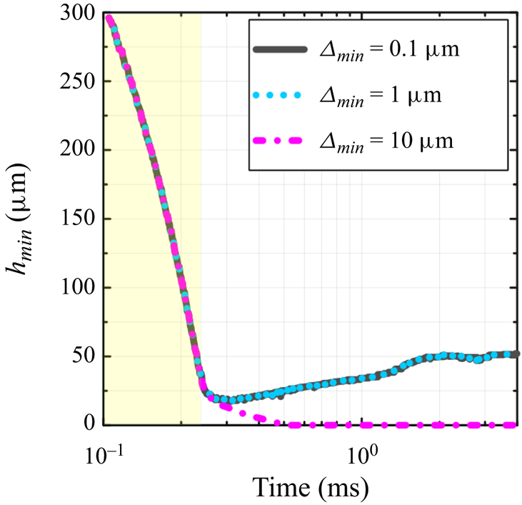
Figure 9 corroborates the arguments below. It illustrates the instantaneous minimal distance between the drop and the bottom wall of the computational box ( $h_{min}$) as a function of time for three different values of
 $\varDelta _{min}$ at
 ${Re} = 17$ and
 ${We} = 72.25$ (typical mixed inertio-viscous-capillary case):
 $0.1\ \mathrm {\mu }\textrm {m}$,
 $1\ \mathrm {\mu }\textrm {m}$ and
 $10\ \mathrm {\mu }\textrm {m}$. The yellow box indicates the initial drop fall (no expansion), which is followed by the drop expansion indicated by the white box. As observed, similar
 $h_{min}$ curves are obtained at
 $\varDelta _{min} = 0.1\ \mathrm {\mu }\textrm {m}$ and
 $\varDelta _{min} =1\ \mathrm {\mu }\textrm {m}$ (similar diameter and energy transfer curves are equally obtained; not shown, for brevity). However, the vapour layer is not able to maintain the drop in levitation when
 $\varDelta _{min} = 10\ \mathrm {\mu }\textrm {m}$. These results give us confidence to fix
 $\varDelta _{min}$ at
 $1\ \mathrm {\mu }\textrm {m}$.
Instantaneous minimal distance between the drop and the bottom wall of the computational box ( $h_{min}$) as a function of time for three different values of
 $\varDelta _{min}$ at
 ${Re} = 17$ and
 ${We} = 72.25$ (typical mixed inertio-viscous-capillary case):
 $0.1\ \mathrm {\mu }\textrm {m}$ (grey solid line),
 $1\ \mathrm {\mu }\textrm {m}$ (blue dotted line) and
 $10\ \mathrm {\mu }\textrm {m}$ (magenta dash-dotted line). The yellow box indicates the initial drop fall (no expansion), which is followed by the drop expansion indicated by the white box.

A.2. Interface capturing
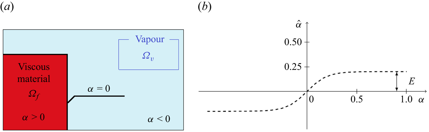
The level-set method, introduced by Osher & Sethian (Reference Osher and Sethian1988), has been applied to numerous two-fluid flows. It consists first in computing the signed distance function to the interface  $\alpha$. As shown in figure 10(a), which describes its initial value, this function is positive in
 $\varOmega _f$ and negative in
 $\varOmega _{vapour}$, where
 $\varOmega$ denotes the computational fluid domain (
 $\varOmega \subset \mathbb {R}^n$, at time
 $t \in [0,T]$). The zero value corresponds to the interface between the two sub-domains:
 \begin{equation} \alpha(\boldsymbol{x}) = \left \lbrace\begin{array}{@{}ll} d(\boldsymbol{x}, \varGamma) , & \boldsymbol{x} \in \varOmega_f , \\ - d(\boldsymbol{x}, \varGamma) , & \boldsymbol{x} \in \varOmega_{vapour} , \\ 0 , & \boldsymbol{x} \in \varGamma . \end{array} \right. \end{equation}
(a) Viscous phase (red) surrounded by a vapour phase (blue). (b) Filtering curve for the level-set function.

Then we need to follow the interface during the simulation. Thus the transport equation of the level-set function should be solved, giving the new interface location:
 \begin{equation} \left \lbrace \begin{array}{@{}l} \dfrac{\partial \alpha}{\partial t}+ \boldsymbol{v} \boldsymbol{\cdot}\boldsymbol{\nabla}\alpha = 0 , \\ \alpha (t=0,\boldsymbol{x})=\alpha_0(\boldsymbol{x}) . \end{array} \right. \end{equation}
This method is often applied in phase transformation and multiphase flows (Osher & Fedkiw Reference Osher and Fedkiw2001; Ji, Chopp & Dolbow Reference Ji, Chopp and Dolbow2002). Indeed, it allows us to describe a wide range of problems, as it can handle problems where the surface evolves in fairly complex ways with high topology changes. Then intrinsic geometric properties of the interface, such as normal vectors or curvatures, are determined from the level-set field. However, some additional treatments, listed below, are necessary to improve the efficiency of this approach.
A.3. Redistancing and filtering of the level-set function
After the resolution of the transport equation (A2), many oscillations may appear close to the interface, polluting the interface quality. Indeed, the isocontours of the level-set function are no longer smooth, leading to the loss of its metric property  $\|\boldsymbol {\nabla } \alpha \|= 1$. Thus a reinitialization step is performed by solving the Hamilton–Jacobi equation to ensure
 $\|\boldsymbol {\nabla } \alpha \| = 1$.
Moreover, during the convection of the level-set function, high gradient changes may occur, giving rise to instabilities and then polluting the final solution. Usually, a filtering function  $\hat {\alpha }$ is defined, equal to zero at the interface, approaching
 $\alpha$ close to the interface, and keeping constant value far from the interface. Several filtering functions can be found in the literature (Olsson & Kreiss Reference Olsson and Kreiss2005; Bonito, Guermond & Lee Reference Bonito, Guermond and Lee2015; Khalloufi et al. Reference Khalloufi, Mesri, Valette, Massoni and Hachem2016). In this work, a hyperbolic tangential filter is used. Thus the new filtered level-set function
 $\hat {\alpha }$ is computed as
 \begin{equation} \hat{\alpha}=E\times \tanh \left( \frac{\alpha}{E} \right), \end{equation}
where  $E$ corresponds to the interface thickness; figure 10(b) shows a typical plot of
 $\hat {\alpha }$, which tends to
 $E$ as
 $\alpha$ increases.
Thus the reinitialization equations can be updated, taking into account the filtered level-set function  $\hat {\alpha }$. The gradient of
 $\hat {\alpha }$ is computed as
 \begin{equation} \frac{\partial \hat{\alpha}(\alpha)}{\partial \alpha} = 1 - \tanh^2 \left( \frac{\alpha}{E} \right), \end{equation}
and is formulated with respect to  $\hat {\alpha }$ as
 \begin{equation} \frac{\partial \hat{\alpha}(\alpha)}{\partial \alpha} = 1 - \left( \frac{\hat{\alpha}(\alpha)}{E} \right)^2. \end{equation}
Then a new fictive step, called  $t_f$, is introduced. The purpose consists in finding a new parametric function
 $\beta$ where the reinitialization step must be performed, and having the same isovalue
 $\alpha$ such that
 \begin{equation} \|\boldsymbol{\nabla} \beta \|= 1 . \end{equation}
The Hamilton–Jacobi equation is then formulated as
 \begin{equation} \left\lbrace \begin{array}{@{}l} \dfrac{\partial \beta}{\partial t_f}+ s(\beta) (\| \boldsymbol{\nabla} \beta \| - 1) = 0, \\ \beta(t_f=0,\boldsymbol{x}) = \alpha(t,\boldsymbol{x}) . \end{array} \right. \end{equation}
Considering now the filtering level-set function  $\hat {\alpha }$, the Hamilton–Jacobi equation becomes
 \begin{equation} \left \lbrace \begin{array}{@{}l} \dfrac{\partial \beta}{\partial t_f}+ s(\hat{\alpha}) \left[\|\boldsymbol{\nabla} \hat{\alpha}\| - \left(1-\left(\dfrac{\hat{\alpha}}{E} \right)^2 \right)\right] = 0, \\ \beta(t_f=0,\boldsymbol{x}) = \alpha(t,\boldsymbol{x}) . \end{array} \right. \end{equation}
By turning (A8) into a transport equation, the problem is rewritten as
 \begin{equation} \left \lbrace \begin{array}{@{}l} \dfrac{\partial \beta}{\partial t_f} + \boldsymbol{U} \boldsymbol{\cdot}\boldsymbol{\nabla} \hat{\alpha} = s(\hat{\alpha}) \left[1-\left(\dfrac{\hat{\alpha}}{E} \right)^2\right], \\ \beta(t_f=0,\boldsymbol{x}) = \alpha(t,\boldsymbol{x}) , \end{array} \right. \end{equation}
with
 \begin{equation} \boldsymbol{U}= \frac{ s(\hat{\alpha})\,\boldsymbol{\nabla} \hat{\alpha}}{\| \boldsymbol{\nabla} \hat{\alpha} \|}. \end{equation}
A.4. Coupling transport and redistancing steps
We couple both the transport and the Hamilton–Jacobi equations (Khalloufi et al. Reference Khalloufi, Mesri, Valette, Massoni and Hachem2016). This step reduces the system to finally one global transport equation, and will consequently eliminate the frequency parameter for the reinitialization. Thus we define  $\lambda$ as the ratio between fictive and real time steps:
 \begin{equation} \lambda = \frac{\partial t_f}{\partial t} . \end{equation}
Then, by choosing  $\lambda$ such that
 $\lambda = {l}/{\triangle t}$, where
 $l$ is the mesh size, one obtains
 \begin{equation} \frac{\partial \beta}{\partial t} = \lambda\,\frac{\partial \beta}{\partial t_f} . \end{equation}
Introducing (A12) in (A9), the new convection-reinitialization equation is obtained:
 \begin{equation} \frac{\partial \beta}{\partial t} + \lambda \boldsymbol{U} \boldsymbol{\cdot}\boldsymbol{\nabla} \hat{\alpha} = \lambda\,s(\hat{\alpha}) \left[1-\left(\frac{\hat{\alpha}}{E} \right)^2\right] . \end{equation}
Therefore, in particular at the interface, the equation that couples the transport and the reinitialization steps will be formulated as
 \begin{equation} \frac{\partial \hat{\alpha}}{\partial t} + (\boldsymbol{u} + \lambda \boldsymbol{U}) \boldsymbol{\cdot}\boldsymbol{\nabla}\hat{\alpha} = \lambda\,s(\hat{\alpha}) \left[1-\left(\frac{\hat{\alpha}}{E} \right)^2 \right] . \end{equation}
This new equation leads to the appearance of a new convection term:  $(\boldsymbol {u}+ \lambda \boldsymbol {U}) \boldsymbol {\cdot }\boldsymbol {\nabla } \hat {\alpha }$. The associated variational formulation is: find
 $\hat {\alpha } \in \mathcal {L}^2(\varOmega )$ such that
 \begin{equation} \left(\frac{\partial \hat{\alpha}}{\partial t}, \varPhi_v \right)_{\varOmega} + \left[ (\boldsymbol{u} + \lambda \boldsymbol{U}) \boldsymbol{\cdot}\boldsymbol{\nabla} \hat{\alpha}, \varPhi_v \right]_{\varOmega} = \left[ \lambda\,s(\hat{\alpha}) \left(1 - \left(\frac{\hat{\alpha}}{E} \right)^2 \right), \varPhi_v \right]_{\varOmega} \end{equation}
for all  $\varPhi _v \in \mathcal {L}^2(\varOmega )$.
The problem is then discretized with respect to time by using a second-order backward differentiation (BFD2) method. Finally, the discretized problem is
 \begin{align} &\left(\frac{3\hat{\alpha}^{n+1} - 4 \hat{\alpha}^n + \hat{\alpha}^{n-1}}{2\,\Delta t}, \varPhi_v \right)_{\varOmega} + \left[ (\boldsymbol{u} + \lambda \boldsymbol{U}) \boldsymbol{\cdot}\boldsymbol{\nabla} \hat{\alpha}^{n+1}, \varPhi_v \right]_{\varOmega} \nonumber\\ &\quad = \left[ \lambda\,s(\hat{\alpha}^n) \left( 1 - \left(\frac{\hat{\alpha}^n}{E} \right)^2\right) , \varPhi_v \right]_{\varOmega} . \end{align}
A.5. Method of resolution – momentum and mass equations
The numerical simulation of viscoplastic flows leads to the resolution of momentum and mass equations (analogue to the incompressible Navier–Stokes equations for Newtonian fluids). The computational fluid domain is defined such that  $\varOmega \subset \mathbb {R}^n$ at time
 $t \in [0,T]$. This problem consists in finding velocity and pressure fields (
 $u$ and
 $p$), defined respectively in the spaces
 $V = \mathbb {R}^n$,
 $P= \mathbb {R}$, such that
 \begin{equation} \left \lbrace \begin{array}{@{}l} \rho \left(\dfrac{\partial \boldsymbol{u}}{\partial t} + \boldsymbol{u} \boldsymbol{\cdot}\boldsymbol{\nabla} \boldsymbol{u}\right) + \boldsymbol{\nabla} p - \boldsymbol{\nabla}\boldsymbol{\cdot}\boldsymbol{\tau} = \boldsymbol{f} , \\ \boldsymbol{\nabla}\boldsymbol{\cdot}\boldsymbol{u} = 0 , \end{array} \right. \end{equation}
where  $\boldsymbol {\tau }$ and
 $\boldsymbol {f}$ correspond respectively to the extra-stress tensor and the source term (here,
 $\boldsymbol {f} = \boldsymbol {f}_{st}$). Recall that the viscous fluid and vapour densities (
 $\rho _f$ and
 $\rho _{vapour}$) and viscosities (
 $\eta _f$ and
 $\eta _{vapour}$) are mixed (into
 $\rho$ and
 $\eta$, respectively) and computed using the Heaviside function of the filtered level-set
 $H(\hat {\alpha })$.