1 Introduction
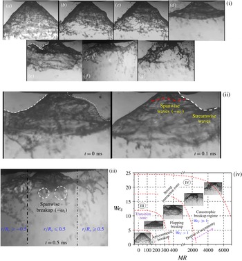
A basic understanding of liquid sheet breakup dynamics and spray formation in swirling flows is of significant interest in many combustion applications (Beér & Chigier Reference Beér and Chigier1972). In particular, in liquid-fuelled gas turbine combustors, optimization of the fuel injection system remains a key challenge (Lefebvre Reference Lefebvre1966). For instance, recent combustors adopt a lean direct injection (LDI) strategy, which utilizes swirling coflowing air to achieve enhanced atomization and a subsequent homogeneous fuel–air mixture prior to combustion (Archer & Gupta Reference Archer and Gupta2003; Marek, Smith & Kundu Reference Marek, Smith and Kundu2005). In these classes of atomizers, the momentum associated with the coflowing air is several orders higher than the liquid flow, resulting in energy transfer from the air to the fuel (Varga, Lasheras & Hopfinger Reference Varga, Lasheras and Hopfinger2003; Fuster et al.
Reference Fuster, Matas, Marty, Popinet, Hoepffner, Cartellier and Zaleski2013). The most important control parameters in this type of geometry are the liquid and gas velocities (
 $U_{l},U_{g}$
) and densities (
 $\unicode[STIX]{x1D70C}_{l},\unicode[STIX]{x1D70C}_{g}$
), represented conveniently as the momentum ratio (MR). Hence, the breakup dynamics of the air-assisted liquid sheet is completely different from that of a simple capillary driven sheet/jet breakup. The review by Lasheras & Hopfinger (Reference Lasheras and Hopfinger2000) highlighted the complexity of identifying the basic mechanism of atomization in air-assisted atomizers. In any atomization process, the droplet formation in the spatial domain is divided into two regimes, namely near field (primary breakup regime) and far field (secondary breakup regime). Most studies analyse the events subsequent to the primary breakup region, namely secondary breakup. The liquid sheet injected into the still/coflowing air environment is subject to instabilities (either shear or surface tension driven) before undergoing breakup in the primary region. Flow visualizations performed by Hoyt & Taylor (Reference Hoyt and Taylor1977) and classical instability studies (Rayleigh 1878; Weber Reference Weber1931) established that in a quiescent gas environment (i.e.
 $U_{g}=0$
), instabilities are more active in the downstream regions rather than near the nozzle. However, in situations where the momentum of the gas phase is higher than that of the liquid phase, instability grows in the primary region itself (i.e. the near field of the nozzle) (Castleman Reference Castleman1931). Hence, in coaxial flows, the spatial distribution of momentum of the two fluids determines the degree of interaction.
Quantitative prediction of droplet size distribution is a subject of interest in any atomizer (Lefebvre Reference Lefebvre1966). Most previous studies (Mugele & Evans Reference Mugele and Evans1951; Xianguo & Tankino Reference Xianguo and Tankino1987; Gu, Basu & Kumar Reference Gu, Basu and Kumar2012) have established the functional relationships between droplet size and flow parameters based on liquid and gas relative velocity, surface tension and injector geometry, among others. However, the underlying mechanism is still an open-ended problem. Hence, it is mandatory to analyse the physical mechanism and spatio-temporal scales, which dominate liquid breakup, drop formation and the corresponding size distributions. Since, in coaxial atomization, the primary energy source is shear between the gas and liquid phases, it leads to KH (Kelvin–Helmholtz) instability at the liquid–gas interface. The destabilization of the interface by the surrounding gas was first studied by Taylor (Reference Taylor1963). It is established that the most unstable wavelength is a linear function of the gas velocity and surface tension. Later, the studies by Dombrowski & Johns (Reference Dombrowski and Johns1963) and Fraser, Dombrowski & Routley (Reference Fraser, Dombrowski and Routley1963) correlated the ligament diameter with the most unstable wavelength (
 $d_{L}\approx (\unicode[STIX]{x1D706}_{max})^{0.5}$
). However, recent experiments carried out by Raynal et al. (Reference Raynal, Villermaux, Lasheras and Hopfinger1997) in a two-phase mixing layer revealed that the primary instability of the liquid–gas interface is dominated by the formation of a boundary/vorticity layer across the interface. The important point to notice is that the wavelength predicted by Raynal et al. (Reference Raynal, Villermaux, Lasheras and Hopfinger1997) contradicts predictions made by Squire (Reference Squire1953) and Dombrowski & Johns (Reference Dombrowski and Johns1963) using the KH instability (without considering the shear layer thickness) dispersion relation. At higher air flow rates, the excess air dynamic pressure (
 $\unicode[STIX]{x1D70C}_{g}U_{g}^{2}\gg \unicode[STIX]{x1D70C}_{l}U_{l}^{2}$
) leads to the formation of vortices in the boundary layer across the interface and results in instabilities at the liquid surface (Lasheras, Villermaux & Hopfinger Reference Lasheras, Villermaux and Hopfinger1998). The most unstable wavelength
 $(\unicode[STIX]{x1D706}_{p})$
in the primary region scales as
 $\unicode[STIX]{x1D706}_{p}\sim \unicode[STIX]{x1D6FF}_{g}\{\unicode[STIX]{x1D70C}_{l}/\unicode[STIX]{x1D70C}_{g}\}^{0.5}$
, where
 $\unicode[STIX]{x1D6FF}_{g}$
is the gas/vorticity layer thickness. Furthermore, at very high air flow rates, studies (Mayer Reference Mayer1994; Zhao et al.
Reference Zhao, Liu, Tian, Xu, Li and Lin2014) have shown negligible effects of surface tension on the primary instability, and the resulting droplet size is well correlated with the air turbulence levels and kinetic energy.
The breakup dynamics and its length scale (i.e. breakup length
 $X_{b}$
) are completely synchronized with dominant air flow instability modes (Lozano, Garcıa-Olivares & Dopazo Reference Lozano, Garcıa-Olivares and Dopazo1998; Park et al.
Reference Park, Huh, Li and Renksizbulut2004). The strong vortices formed around the liquid sheet/jet give rise to the formation of unstable waves in both the streamwise and spanwise directions. In particular, at higher MR values, spanwise waves assume the dominant role and induce catastrophic bag breakup. The large-scale coherent vortices formed at the liquid–gas interface due to impulse disturbances act as the fundamental driving mechanism of ligament detachment from the continuous liquid sheet (Jerome et al.
Reference Jerome, Marty, Matas, Zaleski and Hoepffner2013). Further, in situations where
 $X_{b}$
is larger than the air jet potential core, oscillatory motion of the liquid jet is observed (i.e. flapping) (Matas & Cartellier Reference Matas and Cartellier2013).
To this end, the available literature highlights the primary instability mechanism of liquid jets/sheets in normal air (i.e. non-swirling) jets. However, most practical combustors utilize swirling flows, which have velocity components in both the axial and azimuthal directions and therefore exhibit topological structures that are completely different from those of non-swirling jets (Lilley Reference Lilley1977). In the case of strong swirling jets (
 $S_{G}\geqslant 0.6$
;
 $S_{G}=\text{swirl number}$
), Billant, Chomaz & Huerre (Reference Billant, Chomaz and Huerre1998) and Liang & Maxworthy (Reference Liang and Maxworthy2005) showcased the vortex breakdown mechanism induced by the pressure deficit in the radial direction. This feature causes flow reversal along the jet axis. Hence, swirl flows exhibit axial velocity components in both the positive and negative streamwise directions. In addition, in the region close to the swirler, the strong velocity gradient between the radial and axial velocity components leads to the formation of two counter-rotating vortices. The decay in circulation intensity
 $(\unicode[STIX]{x1D6E4})$
of these vortices in the traverse direction causes vortex shedding at the outer edge. This feature is reported as a precessing vortex core (PVC) in swirling jets (Syred Reference Syred2006).
The combined velocity gradient in the axial and azimuthal directions leads to the evolution of fundamental shear instability (KH instability) in two major forms: one with an axial shear layer and the other with an azimuthal shear layer (Chigier & Chervinsky Reference Chigier and Chervinsky1967). Unlike normal jets, a swirling jet exhibits several distinct modes of flow instability; for instance, weak swirl induces dominant helical modes, and at high swirl levels (
 $S_{G}\sim 0.8$
), the flow becomes centrifugally unstable in the recirculation region (Gallaire & Chomaz Reference Gallaire and Chomaz2003). These instability modes act as primary factors in determining the convective/absolute stability of the secondary jet. In this light, a basic understanding of the pathways involved in the time evolution of the complex topologies of a swirling jet gains significant importance. Swirling jets lead to several fundamental transition modes if secondary flow is introduced. In gas–gas coaxial swirling flow, Santhosh, Miglani & Basu (Reference Santhosh, Miglani and Basu2013) showed that the central jet is completely entrained by swirling coflow, if the velocity deficit is sufficiently high
 $(\unicode[STIX]{x0394}U_{y}\gg 0)$
. Further, the large-scale oscillations of the dominant flow structures exhibit coupling effects with the secondary flow. In addition, the characteristic feature, named the central toroidal recirculation zone (CTRZ) in swirling flows, serves as a determining factor in the stability of secondary flow (Champagne & Kromat Reference Champagne and Kromat2000). In particular, in reacting systems, the CTRZ plays a major role in stability and topological transitions in flames (Santhosh & Basu Reference Santhosh and Basu2015).
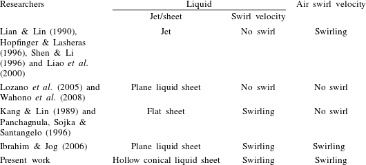
Large-eddy simulation studies carried out by Wang et al. (Reference Wang, Yang, Hsiao, Hsieh and Mongia2007) in a model gas turbine combustor highlighted the dominance of the precessing vortex core in the evolution of swirling flow in the spatial domain. Several studies have highlighted the influence of swirl on the liquid and gas phases (see table 1). For example, Lian & Lin (Reference Lian and Lin1990) showed that swirl introduced to a coflowing gas phase offered a stabilization effect on liquid jet breakup. Classical instability analysis performed by Liao et al. (Reference Liao, Jeng, Jog and Benjamin2000) also displayed the same phenomenon. On the other hand, Kang & Lin (Reference Kang and Lin1989) reported the destabilizing effect of swirl imparted to the liquid phase. Hopfinger & Lasheras (Reference Hopfinger and Lasheras1996) observed a two-way coupling effect, i.e. at low swirl, the recirculation vortex completely disappeared, whereas high swirl induced lateral expansion of the liquid jet followed by explosive breakup. Saha et al. (Reference Saha, Lee, Basu and Kumar2012) also reported weak interaction of a liquid sheet with coannular swirling/ambient air at very low flow rates using low-speed particle image velocimetry (PIV) and shadowgraphy. In a central coaxial atomizer, Ibrahim & Jog (Reference Ibrahim and Jog2006) studied the degree of swirl imposed on both the gas and liquid phases (swirl
 $+$
swirl). Their results showed that the relative swirl strength between the gas and liquid phases greatly enhances the primary instability characteristics.
Coaxial atomization-flow configuration.

1.1 Scope of this paper
The above-presented literature survey in coaxial atomization clearly shows the lack of understanding of the physical mechanisms of atomization in a hollow liquid sheet injected into a swirling gas environment. The main objective of this paper is to gain insights into the momentum transfer coupling between the gas and liquid phases.
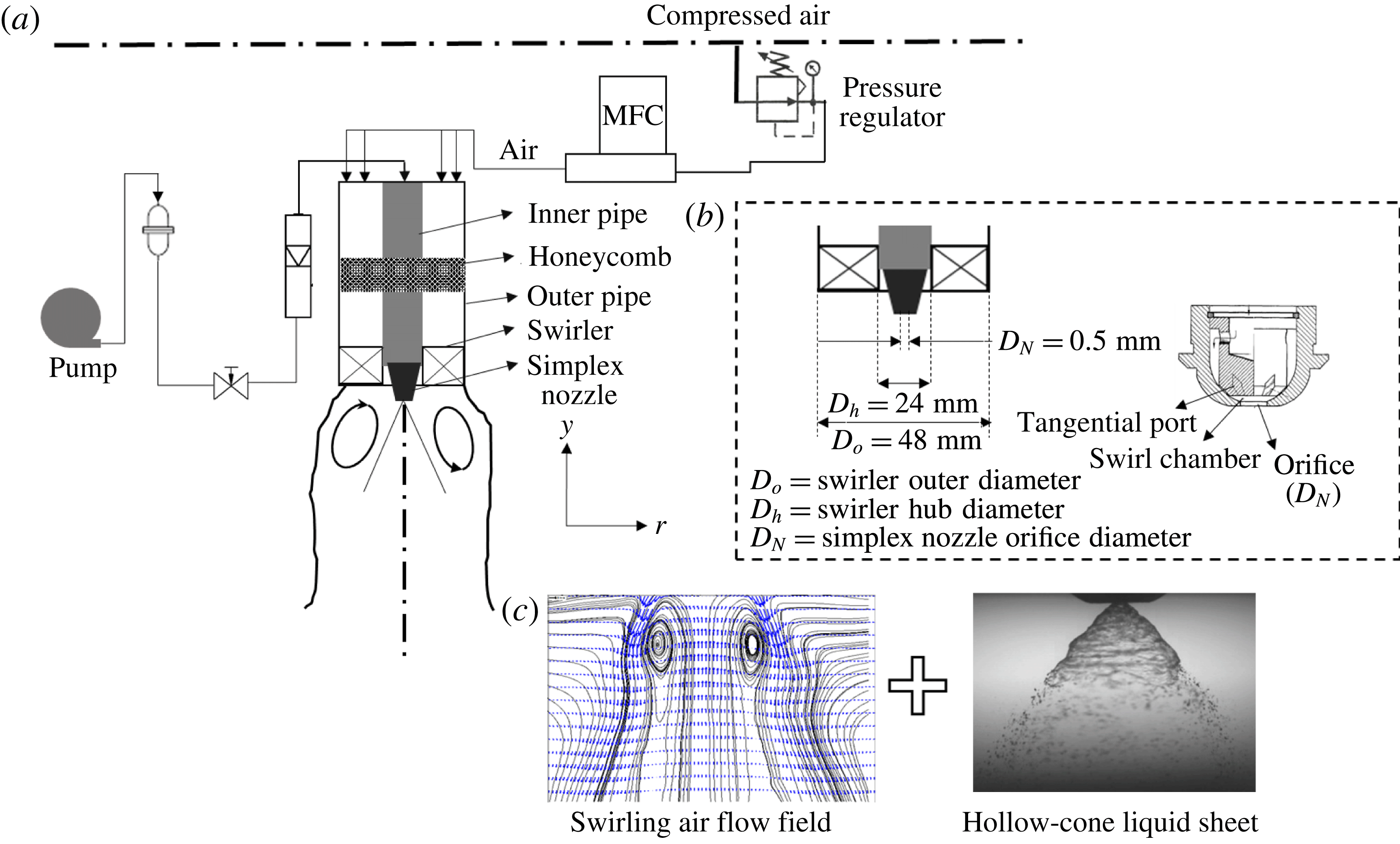
In this work, we consider a flow geometry similar to LDI combustors, i.e. injection of a hollow cone of liquid from a simplex nozzle into a swirling air flow field (see figure 1). The chosen experimental design and flow configuration enable us to study the impact of flow topology (e.g. identification of higher energetic zones in the spatial domain) on primary breakup dynamics and droplet formation. Hence, in our case, the swirling flow field is meticulously analysed using time-resolved PIV (
 $3500~\text{frames}~\text{s}^{-1}$
). This provides insights into the evolution of the topological flow structures in the spatio-temporal domain. Next, high-speed shadowgraphy (
 $20\,000~\text{frames}~\text{s}^{-1}$
) is implemented to capture the effect of the swirling gas phase on the liquid sheet.
In § 2, we explain the flow configurations and optical measurement techniques used in this study. Section 3 describes swirling flow characterization (including the time-averaged velocity profile and the vorticity magnitude) carried out using PIV. Extraction and identification of dominant flow topologies and instability modes using proper orthogonal decomposition (POD) are presented in § 4. Section 5 quantifies the spatial and temporal dynamics of the liquid sheet, momentum transfer coupling and flow transitions between the gas and liquid phases (presented based on a comparison between the liquid sheet and gas phase POD eigenmodes). Linear stability analysis (§ 6) is carried out to understand the evolution of the growth rate for the imposed disturbances. Finally, in §§ 7 and 8, we present how the most unstable wavelength imposed by the swirling air flow field correlates with the breakup dynamics of the liquid sheet and primary drop formation.
2 Experimental conditions and procedure
The experimental set-up (shown schematically in figure 1
a) consisted of a vane swirler and a simplex nozzle arranged in a coaxial configuration. Across all of the experiments, air and water were used as working fluids at atmospheric pressure. Swirling motion was imparted to the air flow through the vane swirler attached at the exit of the outer pipe (figure 1
a). The swirler used here had six vanes with a vane angle of
 $\emptyset =45^{\circ }$
(vane thickness
 $t_{v}=2~\text{mm}$
, swirler outer diameter
 $D_{o}=48~\text{mm}$
, swirler hub diameter
 $D_{h}=28~\text{mm}$
), and the corresponding geometric swirl number (
 $S_{G}$
) was 0.81 (calculated using (3.2)). The conical liquid sheet was generated through the simplex nozzle (with orifice diameter
 $D_{N}=0.5~\text{mm}$
). Honeycombs and pulsation dampers were inserted in the air and liquid flow lines to suppress flow disturbances.
(a) Schematic of the experimental set-up; (b) swirler and simplex nozzle geometry details; (c) flow configuration.

The liquid flow rate was maintained as constant (
 $m_{L}=0.1~\text{l}~\text{min}^{-1}$
,
 $U_{L}=3~\text{m}~\text{s}^{-1}$
) across all of the experiments while the air flow rate was varied from 500 to
 $3000~\text{l}~\text{min}^{-1}$
(
 $U_{g}=9.01~\text{m}~\text{s}^{-1}$
–
 $60~\text{m}~\text{s}^{-1}$
) through a high-precision computer-controlled mass flow controller (M/s., Alicat Inc). The standalone spray was also characterized (no external air flow rate). The liquid flow rate was measured using an inline flow rotameter (range 0–
 $5~\text{l}~\text{min}^{-1}$
, accuracy
 $\pm 0.001~\text{lpm}$
). It should be noted that the spray from the nozzle was generated by pressurizing the liquid using a pump (differential pressure
 $\unicode[STIX]{x0394}p=150~\text{KPa}$
, corresponding sheet velocity
 $U_{L}\sim 3~\text{m}~\text{s}^{-1}$
) without any assistive internal air flow. In the absence of external air flow, the spray exhibited a hollow-cone structure (cone angle of
 ${\sim}85^{\circ }$
), as shown in figure 1(b). In this study, high-speed PIV and shadowgraphy were employed to understand the complex dynamics/interactions between the swirling air flow and the liquid sheet. In addition, phase Doppler interferometer was used to determine the size of the first-generation droplets downstream of the primary breakup regime.
2.1 Methodology and measurements
2.1.1 Time-resolved PIV
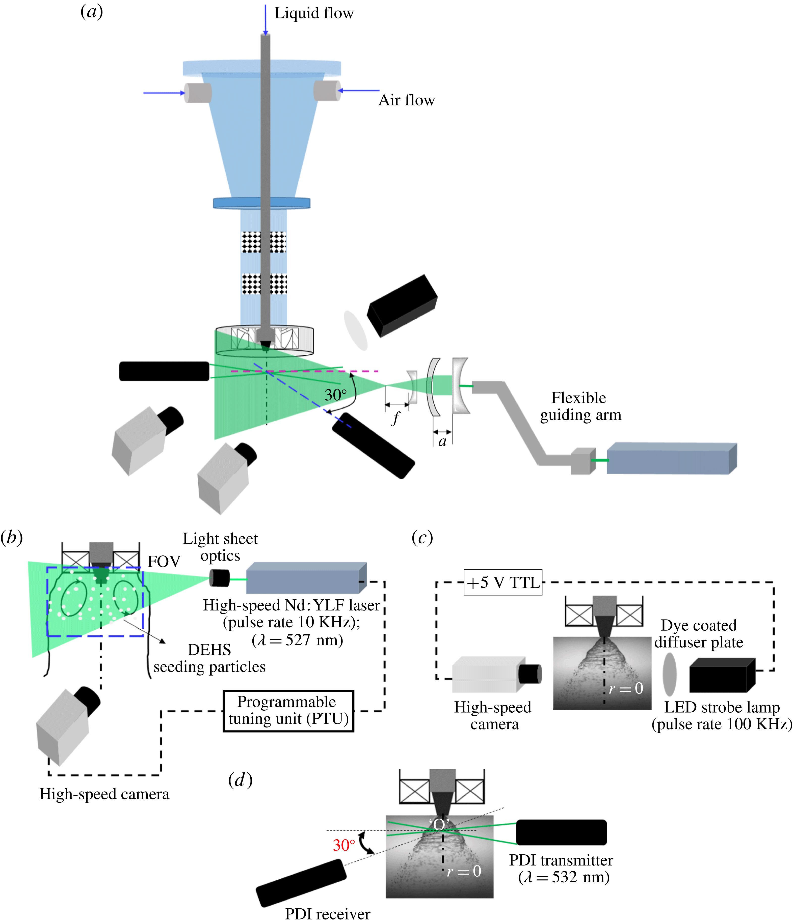
The arrangement of the time-resolved speed PIV system to characterize the swirling air flow field is shown in figure 2(a,b). A dual-pulsed high-speed Nd:YLF laser (repetition rate 10 KHz) with a wavelength of 532 nm and a pulse energy of
 $30~\text{mJ}~\text{pulse}^{-1}$
was used as an illumination source. The cylindrical output beam of the laser (5 mm in diameter) was converted to a thin sheet of 1 mm thickness using a divergent sheet making optics and telescopic lens arrangement (
 $f=-10~\text{mm}$
; see figure 2
a).
(a) Schematic of the diagnostic system; (b) time-resolved (high-speed) PIV; (c) shadowgraphy; (d) phase Doppler interferometry (PDI) system to evaluate droplet size and velocity.

Further, the sheet was properly oriented along the midplane of the coaxial atomizer to illuminate a spatial field of
 $110~\text{mm}\times 110~\text{mm}$
. The flow was seeded with diethyl hexa sebacate (DEHS) oil droplets with the help of an aerosol generator (particle size
 ${\sim}1{-}3~\unicode[STIX]{x03BC}\text{m}$
,
 $\unicode[STIX]{x1D70C}=912~\text{kg}~\text{m}^{-3}$
). The proper seeding density was chosen for each flow condition in such a way that the number of seeding particles per interrogation window was less than 10 (
 $N_{IW}\leqslant 10$
; details can be found in Raffel et al.
Reference Raffel, Willert, Wereley and Kompenhans2013). In this study, a Photron model SA5 (frame rate 7.5 KHz at
 $1024\times 1024$
pixel resolution) camera was used to capture the instantaneous images. The optical axis of the camera was aligned orthogonally to the horizontal axis of the laser sheet. The camera and laser were synchronized via a programmable tuning unit (PTU) to operate in double-frame mode. The pulse separation time (
 $\text{d}t$
) between two frames was chosen based on the optimal shift of particles across the two frames (Keane & Adrian Reference Keane and Adrian1990). Here, the optimal shift was chosen such that the particle shift across the two frames during a short time interval was less than
 $1/4$
of the interrogation window size (i.e.
 $\text{d}x,\text{d}y<IW/4$
). The Stokes number of the seeding particles was maintained at
 $10^{-3}$
to ensure tracing accuracy error within 1 %. For all of the flow conditions, particle images were recorded at
 $3500~\text{frames}~\text{s}^{-1}$
with a spatial resolution of
 $1024\times 1024$
pixels (for a
 $110~\text{mm}\times 110~\text{mm}$
window the magnification factor was chosen as
 $9.3~\text{pixels}~\text{mm}^{-1}$
). Two thousand images were acquired for each experimental condition (acquisition time
 $0.57~\text{s}$
). A 532 nm band-pass filter was coupled to the camera lens to minimize any optical reflection from the metal surfaces of the experimental set-up.
The recorded images were postprocessed using Lavision Davis 8.2 software to reconstruct the vector fields. For all of the test cases, the velocity field was evaluated by dividing the acquired particle images into interrogation window sizes of
 $48\times 48$
pixels. Adaptive PIV was employed to improve the spatial resolution of the vector fields (this technique enables autocalculation of the window shape based on the gradient in the flow field).
2.1.2 High-speed shadowgraphy
High-speed shadowgraphy was employed to study the topological structure of the spray with and without swirling coflow air. Figure 2(b) illustrates the arrangement of the shadow imaging system, consisting of a strobe lamp (IDT-Vision; pulse rate 100 KHz, luminosity 17 000 lm) and a high-speed camera (the same as the one used in PIV) arranged in the same plane. The light from the strobe lamp was made to pass through a dye coated diffuser plate to ensure uniform illumination density.
The flash duration of the strobe lamp was synchronized with the camera shutter speed (through the TTL signal) to acquire the time-frozen snapshots of the spray structures. The images were acquired at
 $20\,000~\text{frames}~\text{s}^{-1}$
with a resolution of
 $704\times 520$
pixels. The spatial field was chosen to be
 $46\times 35~\text{mm}$
, with a magnification factor of
 $15~\text{pixels}~\text{mm}^{-1}$
. Ten thousand images were acquired for each flow condition (0.5 s of temporal data). For imaging of the global structure of the spray, a 100 mm macro lens (Tokino) was used.
A long-distance microscope (with
 $2\times$
magnification lens; Questar model QM1) was coupled to the camera to capture the near-field breakup dynamics. Here, two spatial fields were chosen. In the first case, a spatial field of
 $6~\text{mm}\times 6~\text{mm}$
(with a magnification factor of
 $125~\text{pixels}~\text{mm}^{-1}$
) was used to visualize the sheet profile. In the second case, the spatial field was reduced to
 $3~\text{mm}\times 3~\text{mm}$
to visualize the ligaments and first-generation droplets (the magnification factor was fixed at
 $250~\text{pixels}~\text{mm}^{-1}$
). In addition, measurements were carried at three different axial locations (i.e.
 $y/r_{o}=0.1$
, 0.125, 0.5).
The recorded instantaneous images were further processed in MATLAB (POD, edge detection, binarization) to determine the dynamics associated with the breakup. The steps involved in the processing will be explained later in relevant sections.
2.1.3 Phase Doppler interferometry
A one-dimensional PDI system (Atrium Technologies Inc.) was employed to quantify the effect of coflowing swirling air on the sizes and velocities of droplets near the primary breakup region. To achieve this, the two laser beams from the PDI transmitter were aligned along the axis (
 $r=0$
) of the simplex nozzle. The receiver was placed at an angle of
 $30^{\circ }$
off the axis from the intersection point (marked as point ‘O’ in figure 2
d). Since the focal length of the lens used in this study was 500 mm, both units (transmitter and receiver) were placed 500 mm apart from the beam crossover point. At each flow condition, the sharpness of the fringe pattern was ensured. Subsequently, the Doppler signals were monitored using an oscilloscope to check the optical alignment of the system.
In the current set of experiments, the scattering mode was chosen as refraction, since the working medium was transparent (i.e. water). Furthermore, the off-axis forward-scattering mode was employed, due to its improved sensitivity to the droplets (Albrecht et al.
Reference Albrecht, Damaschke, Borys and Tropea2013). The transmitter and receiver units were mounted on a traverse system to probe different measurement locations. Measurements were made at three axial locations (
 $y/r_{o}=0.1$
, 0.125, 0.5) across the transverse axis of the spray (i.e. from the centreline (
 $r=0$
) to the edge of the spray). The acquired fringe patterns were processed using a standalone signal processing unit to reconstruct the droplet size and velocity (Bachalo Reference Bachalo1980; Bachalo & Houser Reference Bachalo and Houser1984) distributions.
2.2 Flow parameters
Primarily, the experiments are characterized by two non-dimensional numbers: the air flow Reynolds number
 $(Re_{g})$
and the air to liquid MR,
 $$\begin{eqnarray}\displaystyle & \displaystyle Re_{g}=\frac{\unicode[STIX]{x1D70C}_{g}U_{g}D_{a,eff}}{\unicode[STIX]{x1D707}_{a}}, & \displaystyle\end{eqnarray}$$
 $$\begin{eqnarray}\displaystyle & \displaystyle Re_{l}=\frac{\unicode[STIX]{x1D70C}_{l}U_{l}D_{l,eff}}{\unicode[STIX]{x1D707}_{l}}, & \displaystyle\end{eqnarray}$$
 $$\begin{eqnarray}\displaystyle & \displaystyle D_{a,eff}=(D_{o}-D_{h})-0.5n_{v}t_{v}, & \displaystyle\end{eqnarray}$$
 $$\begin{eqnarray}\displaystyle & \displaystyle MR=\frac{\unicode[STIX]{x1D700}_{a}}{\unicode[STIX]{x1D700}_{l}}, & \displaystyle\end{eqnarray}$$
where
 $\unicode[STIX]{x1D700}_{a}$
is the air momentum
 $(\unicode[STIX]{x1D70C}_{a}U_{a}^{2}A_{a,eff})$
,
 $\unicode[STIX]{x1D700}_{l}$
is the liquid momentum
 $(\unicode[STIX]{x1D70C}_{l}U_{l}^{2}A_{l,eff})$
,
 $\unicode[STIX]{x1D70C}_{a}$
and
 $\unicode[STIX]{x1D70C}_{l}$
are the air and liquid densities (
 $\text{kg}~\text{m}^{-3}$
),
 $U_{a}$
and
 $U_{l}$
are the mean air and liquid velocities at the exit,
 $D_{a,eff}$
and
 $D_{l,eff}$
are the effective swirler exit diameter for air flow and the effective diameter for liquid flow,
 $n_{v}$
is the number of vanes,
 $t_{v}$
is the vane thickness,
 $A_{eff}$
is the effective area of the air and liquid flow path and
 $\unicode[STIX]{x1D707}_{a}$
is the air viscosity (Pa s). In general, most researchers have neglected the area ratio term in the MR expression (2.4) in the context of coaxial atomization, particularly near the nozzle exit plane. However, it is important to consider the effective liquid flow cross-section in geometries like hollow-cone atomizers. This is because the flow area occupied by the liquid sheet in this configuration is usually 40 % of the total orifice.
The area ratio, however, has been used in the MR expression in a few studies (Engelbert, Hardalupas & Whitelaw Reference Engelbert, Hardalupas and Whitelaw1995; Lozano et al.
Reference Lozano, Barreras, Siegler and Löw2005; Wahono et al.
Reference Wahono, Honnery, Soria and Ghojel2008; Duke, Honnery & Soria Reference Duke, Honnery and Soria2010). The advantage of including the area ratio lies in the precise representation of the relative momentum associated with coflowing fluids. For instance, the value of the MR will be less than 1 (for all of the test cases considered here) if the area ratio is not included in the present study, even though the cross-sectional area for swirling air is much higher than that of the liquid
 $(A_{a}/A_{l}\sim 8700)$
. This implies weak interaction or less dominance of the gas flow in atomization, which is obviously incorrect or misleading. Hence, to represent the degree of interaction accurately, the area ratio is included in MR calculations in this study. It is to be noted that any representation of the MR (with or without the area ratio) does not alter the physical mechanisms of the interactions as represented in this work.
The axis length scales (
 $y,r$
) (figure 1
a) are non-dimensionalized with the swirler outer annulus radius (
 $R_{o}$
).
Since PIV was carried out only for air flow, the results are presented as a function of the air Reynolds number
 $(Re_{g})$
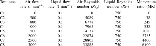
. However, spray diagnostics were carried out with and without air flow. Hence, the MR is used to represent the spray–swirl interaction results (i.e. combined liquid and gas phases). The test cases used in the present experiments are detailed in table 2.
Experimental test cases.

3 Characterization of the outer swirling air flow field
This section describes the detailed investigation of the spatio-temporal structures of the swirling air flow field (without spray) for
 $Re_{g}$
values ranging from 5000 to 35 000. First, we present the instantaneous and time-averaged parameters: vorticity contours (
 $\unicode[STIX]{x1D714}_{z}$
), streamlines, and radial and axial velocity magnitude plots. Subsequently, POD is carried out to represent the dominant instability modes. In addition, we analyse the modal energy distribution and power spectrum density (PSD) of temporal modes which represent the most unstable frequencies for each mode.
3.1 Global observations
In general, swirl flows are characterized by a non-dimensional number named the swirl number (
 $S$
), which is defined as the ratio of the axial flux of tangential momentum to the axial flux of axial momentum,
 $$\begin{eqnarray}S=\frac{\displaystyle \int _{R_{h}}^{R_{o}}\unicode[STIX]{x1D70C}_{a}U_{y}U_{w}2\unicode[STIX]{x03C0}r^{2}\,\text{d}r}{R_{o}\displaystyle \int _{R_{h}}^{R_{o}}\unicode[STIX]{x1D70C}_{a}U_{y}^{2}2\unicode[STIX]{x03C0}r\,\text{d}r},\end{eqnarray}$$
where
 $U_{w}$
and
 $U_{y}$
are the angular and axial velocity components respectively. However, for the class of swirler geometry (i.e. axial flow flat-vane swirler) used in the current experimental work, the ratio of azimuthal to axial velocity is fixed, irrespective of inlet flow conditions (Beér & Chigier Reference Beér and Chigier1972). Hence, it is prudent to represent the flow using the geometric swirl number, which is defined as
 $$\begin{eqnarray}S_{G}=\frac{2}{3}\left[\frac{1-\left({\displaystyle \frac{d_{h}}{d_{o}}}\right)^{3}}{1-\left({\displaystyle \frac{d_{h}}{d_{o}}}\right)^{2}}\right]\tan \emptyset .\end{eqnarray}$$
Here,
 $d_{o}$
and
 $d_{h}$
are the swirler outer and hub diameters.
Hence, for fixed-geometry flat-vane swirlers, the swirl number
 $S_{G}$
can be varied by altering the vane angle
 $\emptyset \;(S_{G}\approx 2/3\tan \emptyset )$
. In our experiments, based on expression (3.2), the geometric swirl number is found to be 0.81. The flow-based swirl number (
 $S$
, from (3.1)) is evaluated to be
 $0.79\pm 0.07$
(for all
 $Re_{g}$
values) based on experimental data.
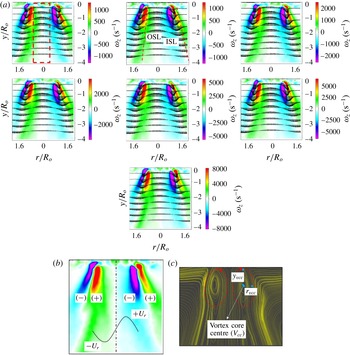
From figure 3(a), it is clear that the time-averaged vorticity
 $(\unicode[STIX]{x1D714}_{\boldsymbol{z}})$
and velocity contours appear to be identical in a topological sense for all
 $Re_{g}$
values. This is due to the fact that the swirler used in this experiment is of fixed-vane type (Gupta, Lilley & Syred Reference Gupta, Lilley and Syred1984). However, a progressive rise in vorticity and velocity magnitudes is observed with increase in
 $Re_{g}$
.
Another noticeable point is the asymmetrical distribution of vorticity contours in swirling jets (figure 3
b). Furthermore, at the critical swirl number
 $(S_{G}\geqslant 0.6)$
, the combined effects of azimuthal and axial shear result in transition from pre-vortex bubble breakdown to a fully developed CTRZ. In the present experiments, since we used
 $S_{G}\sim 0.81$
, a strong CTRZ with a low-velocity vortex core centre (
 $V_{cc}$
) is observed in the near field (
 $y/R_{o}\leqslant 1$
) of the swirler for all flow conditions (i.e. length scales and flow field look identical in all sub cases of figure 3(a) (Chigier & Chervinsky Reference Chigier and Chervinsky1967; Billant et al.
Reference Billant, Chomaz and Huerre1998)). Further, this counter-rotating recirculating core induces an adverse pressure gradient along the jet axis and causes flow reversal (in the region
 $-0.5<r/R_{o}<0.5$
, figure 3
a) in the upstream regions. Subsequently, the flow reversal phenomenon leads to the formation of an inner shear layer (ISL) with streamwise flow in addition to the outer shear layer (OSL) formed with ambient fluid (see figure 3
a; also see supplementary movie 1 available at https://doi.org/10.1017/jfm.2016.710).
(a) Time-averaged vorticity contours (
 $\unicode[STIX]{x1D714}_{\boldsymbol{z}}$
) superimposed with the 2D vector field (from left to right,
 $Re_{g}$
corresponds to test cases C2–C8). (b) Illustration of the asymmetrical time-averaged vorticity distribution. (c) Streamline plot for
 $Re_{g}=33\,888$
. (See movie 1 for instantaneous flow fields at
 $Re_{g}=33\,888$
.)

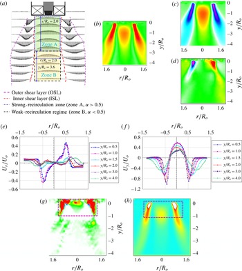
Flow field and velocity distribution. (a,b) Average velocity
 $(|\boldsymbol{V}|)$
vector fields and contours; (c,d) time-averaged axial and radial velocity distribution; (e,f) axial and radial velocity magnitude at different axial locations; (g,h) time-averaged shear strength
 $(\unicode[STIX]{x1D6FD})$
and turbulent kinetic energy (all cases correspond to
 $Re_{g}=33\,888$
).

3.2 Flow regimes
This section presents the flow regimes observed spatially throughout the flow field. Two essential parameters, vital in the context of coaxial atomization in combustion applications, are considered, namely the internal recirculation zone and the shear strength. The parameter velocity ratio
 $\unicode[STIX]{x1D6FC}=|\boldsymbol{V}|/U_{o}$
(where
 $|\boldsymbol{V}|$
is the average velocity in region
 $((r/R_{o})(y/R_{o}))$
and
 $U_{o}$
is the average bulk velocity at the swirler exit) is used to define the strength of the recirculation zone. For instance, the region
 $0<y/R_{o}<2$
(figure 4
a–c) is identified as the strong-recirculation zone (
 $\unicode[STIX]{x1D6FC}>0.5$
; zone A). In zone A,
 $\unicode[STIX]{x1D6FC}$
indicates that more than half of the bulk momentum available at the swirler exit is contributed towards flow reversal. However, the intensity of recirculation is progressively reduced downstream of the jet axis, i.e.
 $y/R_{o}>2$
(
 $\unicode[STIX]{x1D6FC}<0.5$
; zone B). This trend can be explained with the help of the radial velocity distribution. It is seen that in the region
 $0<y/R_{o}<1$
(figure 4
e,f), opposite signs in the radial velocity
 $(-0.5<r/R_{o}<0.5)$
induce a strong pressure deficit along the jet axis. In the far field (
 $y/R_{o}>1$
), the magnitude of the radial velocity is reduced abruptly, which results in weakening of the flow reversal phenomenon.
In coaxial atomization, shear in the air is considered as a primary source of atomization. Hence, the distribution of shear in the spatial field is important, to identify the optimal location for liquid sheet injection. This parameter can be analysed from the vector field. This can be evaluated from the imaginary part of the eigenvalues
 $(\unicode[STIX]{x1D6FD})$
of the velocity Jacobian matrix
 $\left(\!\begin{smallmatrix}\unicode[STIX]{x1D61C}_{rr} & \unicode[STIX]{x1D61C}_{ry}\\ \unicode[STIX]{x1D61C}_{yr} & \unicode[STIX]{x1D61C}_{yy}\end{smallmatrix}\!\right)$
(see (3.3), where
 $i=r$
,
 $j=y$
),
 $$\begin{eqnarray}\unicode[STIX]{x1D6FD}=\frac{\{\unicode[STIX]{x2202}\unicode[STIX]{x1D61C}_{r}/\unicode[STIX]{x2202}y\times \unicode[STIX]{x2202}\unicode[STIX]{x1D61C}_{y}/\unicode[STIX]{x2202}r-\{\unicode[STIX]{x2202}\unicode[STIX]{x1D61C}_{r}/\unicode[STIX]{x2202}r\times \unicode[STIX]{x2202}\unicode[STIX]{x1D61C}_{y}/\unicode[STIX]{x2202}y\}\}}{2}+\frac{\{(\unicode[STIX]{x2202}\unicode[STIX]{x1D61C}_{r}/\unicode[STIX]{x2202}r)^{2}+(\unicode[STIX]{x2202}\unicode[STIX]{x1D61C}_{y}/\unicode[STIX]{x2202}y)^{2}\}}{4}.\end{eqnarray}$$
Figure 4(g) shows the spatial distribution of shear strength. Here, the strength is more concentrated in the region indicated as
 $0<y/R_{o}<1$
;
 $-1<r/R_{o}<1$
because of the strong gradient between the axial and radial velocity components. The interaction between solid body rotation and the perturbations induced by outside flow results in strong shear. Subsequently, this layer is perturbed by combined azimuthal and axial waves. Furthermore, the shrinkage of the streamlines in the radial direction causes a dynamic pressure gradient in this zone. These perturbations in the dynamic pressure result in shear instability. Interestingly, the same region exhibits high average turbulent kinetic energy (figure 4
h).
4 Proper orthogonal decomposition of the swirling flow field
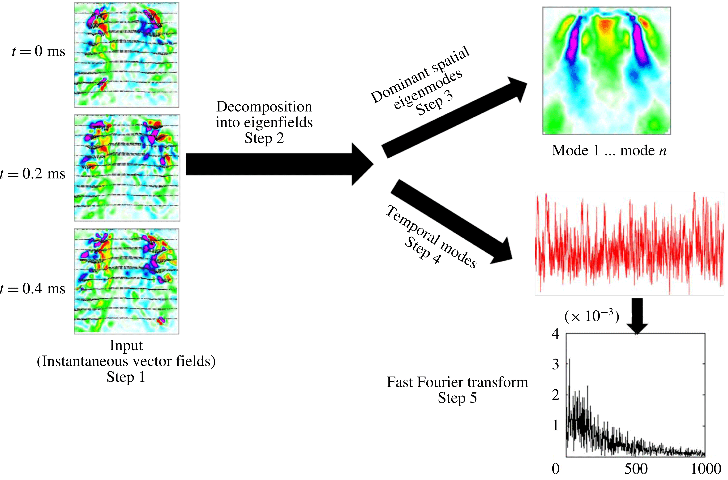
Although time-averaged vector fields and vorticity contours help to identify the global features like strong and weak shear, the instability mechanisms are not clearly understandable. The method of snapshots algorithm (Sirovich Reference Sirovich1987; Holmes, Lumley & Berkooz Reference Holmes, Lumley and Berkooz1998) is utilized to compute the POD modes from the instantaneous vector images (as shown in figure 5).
Steps involved in POD.

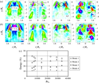
Spatial eigenmodes (a)
 $Re_{g}=5089$
, (b)
 $Re_{g}=33\,888$
: A1 (mode 1), KH (shear
 $+$
strong central circulation); A2 (mode 2), KH (strong shear); A3 (mode 3), helical mode; A4 (mode 4), vortex shedding mode. (c) Modal energy distribution.

The essential role of POD is to extract the dominant flow structures from the velocity cross-correlation matrix
 $[u]_{m\times n}$
, where
 $n$
is the number of image samples and
 $m$
represents the number of velocity data per sample. The first step is to decompose the given number of instantaneous vector fields ‘
 $n$
’ (i.e. snapshots) into summation of the products of spatial eigenmodes
 $\unicode[STIX]{x1D719}_{n}(x)$
and temporal modes
 $a_{n}(t)$
(see (4.1), where
 $N$
is the number of eigenmodes and
 $r_{k}$
is the rank of the correlation matrix). Later, from the velocity matrix eigenvalues,
 $\unicode[STIX]{x1D706}_{n}$
corresponding to each eigenfunction
 $\unicode[STIX]{x1D719}_{n}$
can be evaluated (here,
 $\unicode[STIX]{x1D706}_{n}$
represents the turbulent kinetic energy (TKE)). Subsequently, the percentage of TKE
 $(\unicode[STIX]{x1D706}_{n}/\sum _{i=1}^{4}\unicode[STIX]{x1D706}_{n})$
is calculated to evaluate the modal energy distribution. Furthermore, temporal signatures (step 4) are computed to delineate the most unstable frequency associated with each spatial eigenmode,
 $$\begin{eqnarray}u_{x,t}=\mathop{\sum }_{N=1}^{r_{k}}\unicode[STIX]{x1D719}_{n}(x)a_{n}(t).\end{eqnarray}$$
4.1 Proper orthogonal decomposition spatial modes
Figure 6(a,b) depicts the four dominant (spatial eigenmodes 1–4) instability modes which govern the flow field. The modal mechanisms can be identified based on the vorticity contours (i.e. based on their sign). Only the dynamics of the first four POD modes have been considered based on the energy budget, as shown in figure 6(c). It can be seen that the first four modes cumulatively contribute towards 95 % of the total energy. For instance, vorticity is distributed in a symmetric manner in modes 1 and 2 (figure 6
a,b, A1, A2) across the longitudinal axis (
 $y/r_{o}$
). This symmetrical distribution of vorticity induces rollup of vortical waves along the shear layers (both the ISL and the OSL), leading to KH instability. On the other hand, asymmetrical vorticity contours across the
 $y/r_{o}$
axis (figure 6
a,b, A3), induced by rotation, create helical waves (mode 3). Finally, shedding can also be induced by the PVC at the edge (see figure 6
a,b, A4, mode 4) in the streamwise direction. In general, the identified mechanisms are strong functions of the swirl intensity. However, since the swirl number is constant, the spatial eigenmodes look identical across all flow conditions. In all four spatial eigenmodes, KH instability shows dominance (modes 1 and 2) due to the presence of strong shear induced by the ISL (figure 4
b) and the OSL (figure 3
a) in the axial and azimuthal directions. The occurrence of negative vorticity (circulation in mode 1) in the region
 $-0.5\leqslant r/R_{o}\leqslant 0.5$
is due to the inherent centrifugal effects
 $(\unicode[STIX]{x2202}U_{y}/\unicode[STIX]{x2202}r<\unicode[STIX]{x2202}U_{r}/\unicode[STIX]{x2202}y)$
in swirling jets (i.e. combination of azimuthal and axial shear). Rayleigh’s inviscid criterion states that the shear layer becomes unstable if the circulation intensity decreases in the radially outward direction (i.e. stratification in angular momentum),
 $$\begin{eqnarray}\frac{\text{d}\unicode[STIX]{x1D6E4}}{\text{d}r}<0.\end{eqnarray}$$
Theoretical work by Coles (Reference Coles1965) highlights the centrifugal instability criteria based on the vorticity magnitude and angular velocity, as given in (4.3),
 $$\begin{eqnarray}\unicode[STIX]{x1D714}_{z}\unicode[STIX]{x1D6FA}<0.\end{eqnarray}$$
Hence, the flow becomes centrifugally unstable in the region where
 $\unicode[STIX]{x1D714}_{z}<0$
. The mode 1 vorticity contours shown in figure 6(a,b, A1, A2) clearly depict the formation of negative
 $\unicode[STIX]{x1D714}_{z}$
values near the ISL and OSL due to reduction in circulation intensity along the traverse direction (
 $r/R_{o}$
). This zone is hence identified as centrifugally unstable, leading to flow reversal towards the upstream region. As a result, the dominant KH instability evolves into two forms. One is due to azimuthal shear, which increases due to the combination of KH and circulation (mode 1). The other form corresponds to a pure KH mode (mode 2). However, these events will be true only in strong swirling jets (i.e.
 $S_{G}\geqslant 0.6$
), as in the current experiments.
The majority of the total energy is distributed among KH modes (accounting for
 ${\sim}70{-}80\,\%$
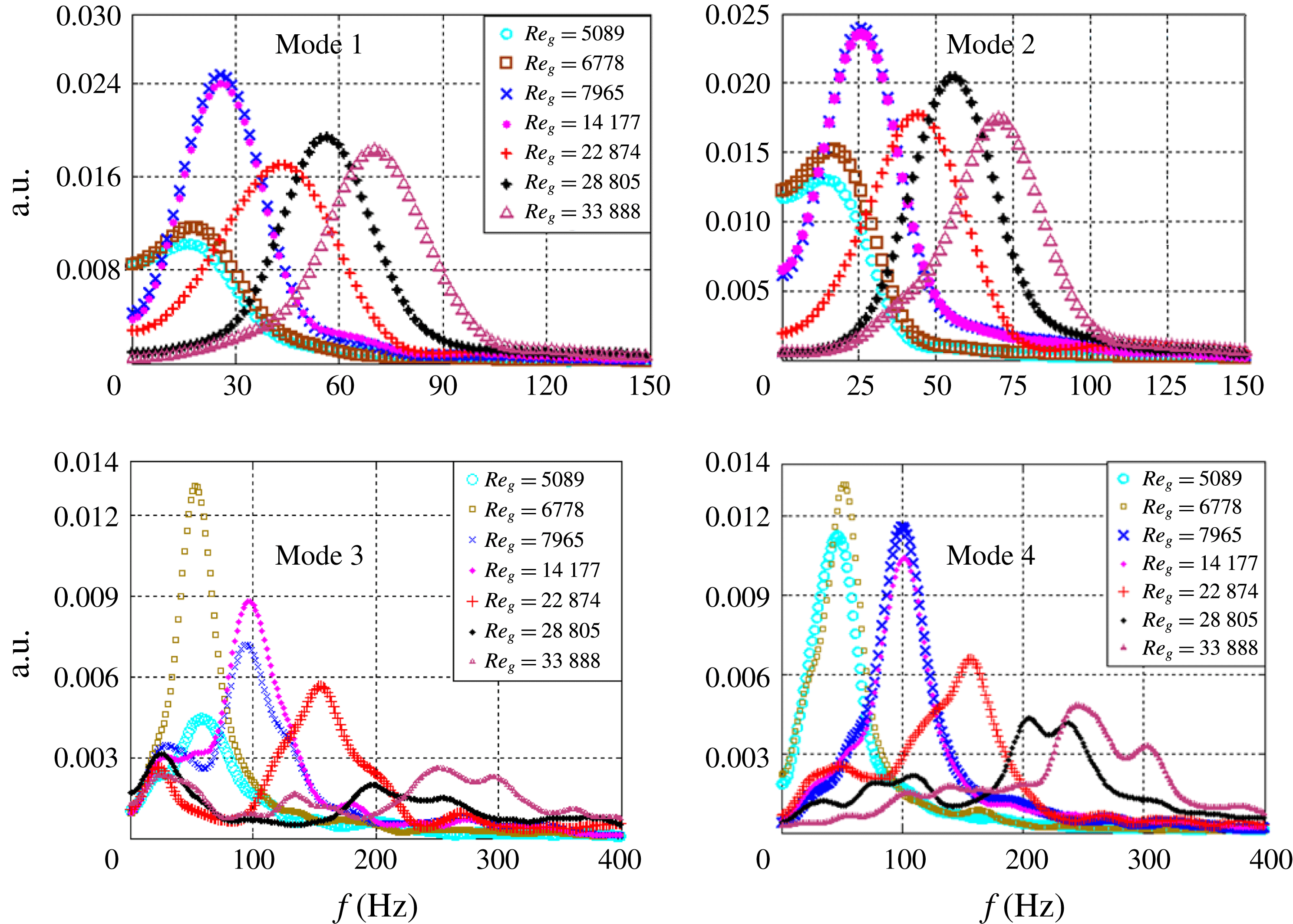
of the total energy), whereas helical and vortex shedding modes account for the other 20 %. The total energy budget and its distribution can be explained based on the PSD analysis of the temporal signatures of the eigenmodes. The frequency peaks are shifted to higher values with increasing air flow rates for all of the modes. In addition, the mode 1 and 2 frequency distributions show narrow half-widths (figure 7
a,b); this may be due to the existence of a single dominant eddy in KH modes implying decay or smaller growth rate for other eddies. This can also imply a lower probability of vortex coupling among different eddies. In contrast, shedding and helical modes (figure 7
c,d) give rise to a multimodal frequency spectrum with a much wider half-width. This implies a wider distribution of energy over a range of wavelengths. In particular, in modes 3 and 4, the frequency peaks are shifted more towards higher values at
 $Re_{g}\geqslant 22\,874$
. In these conditions, the reconstructed instantaneous vector fields suggest increased strength of the precessing vortex core which leads to oscillations of the flow at the edge of the PVC. The narrow frequency spectrum of modes 1 and 2 contributes towards a higher fraction of the total energy compared with modes 3 and 4 (see figure 6
c). These frequency trends clearly show that the most unstable wavelength associated with KH modes (1 and 2) is longer compared with modes 3 and 4 (i.e.
 $\unicode[STIX]{x1D706}_{max,KH}>\unicode[STIX]{x1D706}_{3,4}$
).
The four instability mechanisms and the corresponding dynamics can be summarized as follows.
-
(i) The axial shear layer formed at the ISL and OSL gives rise to KH instability (mode 1).
-
(ii) The flow becomes centrifugally unstable in the region where the circulation intensity (
 $\unicode[STIX]{x1D6E4}$
) decreases (mode 2).
-
(iii) Helical waves (mode 3) are formed due to the influence of the azimuthal velocity component in swirling jets. In swirling jets, helical waves are more active before the occurrence of vortex breakdown. However, in this study, all flow conditions correspond to vortex breakdown. Hence, helical modes do not contribute towards a significant fraction of the total energy budget.
-
(iv) Flow oscillations induced at the reverse flow boundary (i.e. ISL) are depicted as the vortex shedding mode (mode 4). These oscillations may originate from the PVC.

Power spectrum density for POD temporal modes as a function of
 $Re_{g}$
.

5 Spray characterization
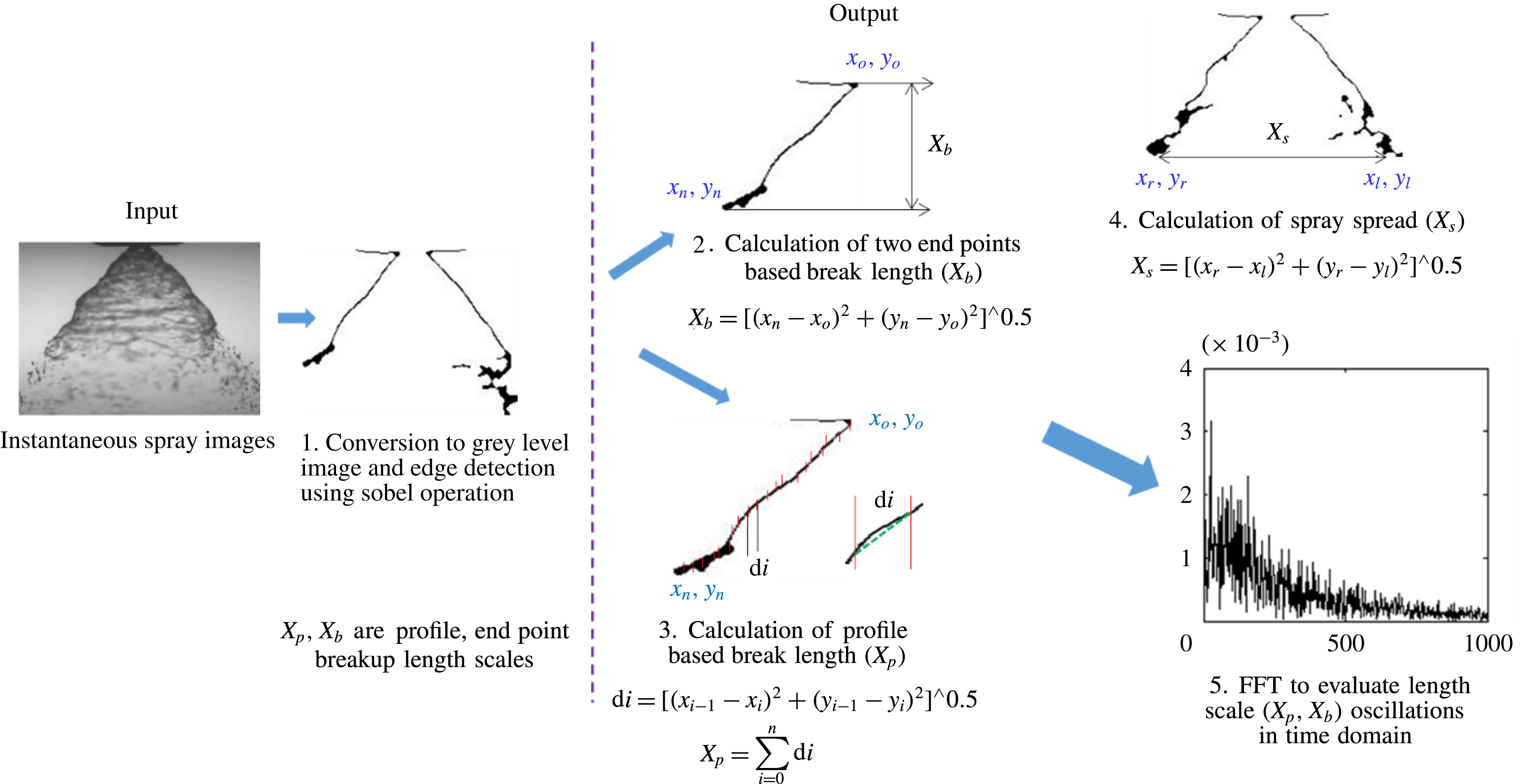
This section outlines the detailed spray characterization carried out using high-speed shadowgraphy. Proper orthogonal decomposition is implemented on the high-speed spray contours to quantify how the swirling air flow affects the dynamics of the liquid sheet. Subsequently, an edge detection technique is implemented on instantaneous liquid sheet images to understand the variations in the global structure of the spray in the presence of outer swirling air. Here, we used the sobel edge detection algorithm in MATLAB. It involves conversion of a given image into
 $3\times 3$
kernels in the form of derivatives in the
 $x$
and
 $y$
directions. Subsequently, the computed
 $x$
,
 $y$
derivatives are multiplied by the source image, yielding the edge of the image (i.e. the contours of the liquid sheet).
5.1 Spray morphology, transition and regimes
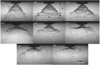
For all of the cases (figure 8
a–h) shown here, the liquid velocity is
 $U_{l}=3~\text{m}~\text{s}^{-1}$
and the air velocity
 $U_{g}$
is varied from
 $9~\text{m}~\text{s}^{-1}$
to
 $60.5~\text{m}~\text{s}^{-1}$
(
 $5000<Re_{g}\leqslant 33\,888$
). It is perceived that there is no significant change in the global spray structure (figure 8
a–c) for lower air flow rates (
 $Re_{g}<7000$
;
 $MR<300$
); however, the effect is more pronounced (figure 8
e–h) for higher air flow rates (
 $14\,000<Re_{g}\leqslant 33\,888$
;
 $MR>1080$
).
Instantaneous visualization of the liquid sheet profile: (a)
 $MR=0$
; (b)
 $MR=138$
; (c)
 $MR=245$
; (d)
 $MR=338$
; (e)
 $MR=1080$
; (f)
 $MR=2785$
; (g)
 $MR=4400$
; (h)
 $MR=6100$
. (See movies 2–4 for visualization of the dynamics of the spray.)

It is to be noted that the spray is symmetric about the nozzle axis, particularly for
 $MR\leqslant 338$
. This symmetry is lost for
 $MR\geqslant 338$
.
The conical liquid sheet injected into the quiescent environment (i.e. without swirling air) is subjected to aerodynamic disturbances, and the unstable waves grow on the surface of the liquid sheet (see figure 8
a). Subsequently, these sheets break into ligaments/droplets in the streamwise direction. In particular, at
 $MR=0$
, the waves formed on the liquid sheet are of Rayleigh type and small in magnitude. The critical length scales, which characterize the global features of the liquid sheet, are the breakup/intact length (
 $X_{b}$
) and lateral spread (
 $X_{S}$
). Furthermore, these length scales exhibit similarity across the time domain. However, in coaxial air-assisted flows, non-similarity and fluctuations cause the liquid sheet behaviour to be more violent and dynamic in nature (see figure 8
d–h). This is due to the fact that, at critical flow conditions, the large-scale coherent structures of the air flow try to exchange momentum with the liquid phase. Hence, the air phase dynamics dominates and disrupts the liquid phase. As a result, the liquid phase starts to mimic the air phase dynamics (strong correlation, as will be explained later).
5.2 Proper orthogonal decomposition modal contributions and characteristic frequencies
It is necessary to identify the mechanism by which momentum transfer happens in coaxial atomization to determine the dynamics of the length scales (
 $X_{b}$
,
 $X_{S}$
). Hence, POD analysis is performed to elucidate the instability modes. The steps involved in computing the liquid phase POD are the same as the ones shown in figure 5, but instead of vector images, instantaneous spray images are used as inputs. Hence, the modal contours obtained for the liquid phase are representations of the spray structure.
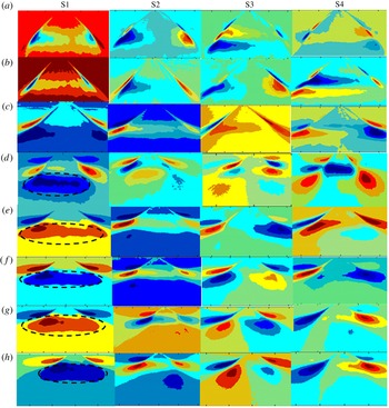
The processed spatial eigenmodes (S1–S4) are schematically shown in figure 9, by superimposing the gas phase eigenmodes (figure 6
a,b) with the liquid phase (see figure 9
a–h). Figure 9(a–c) (low MR, low air flow rate) depicts weak momentum coupling, i.e. the spatial modes of the gas and liquid phases are significantly different. Interestingly, the flow condition
 $MR\geqslant 338$
shows good similarity among the spatial modes (i.e. S1–S4 with A1–A4) with respect to topology. In particular, the central circulation shown by the
 $-\unicode[STIX]{x1D714}_{z}$
region in mode I of the air flow field is completely imposed on the liquid sheet (marked as black dotted lines in S1 of figure 9
d–h). Visually also, this agrees well with the spray images as shown in figure 8(d–h) (intense coupling). The degree of interaction and individual modal contribution in momentum coupling is explained based on the energy and unstable frequencies of the spray eigenmodes.
Combined air and liquid phase POD modes: (a)
 $MR=0$
; (b)
 $MR=138$
; (c)
 $MR=245$
; (d)
 $MR=338$
; (e)
 $MR=1080$
; (f)
 $MR=2785$
; (g)
 $MR=4400$
; (h)
 $MR=6100$
.

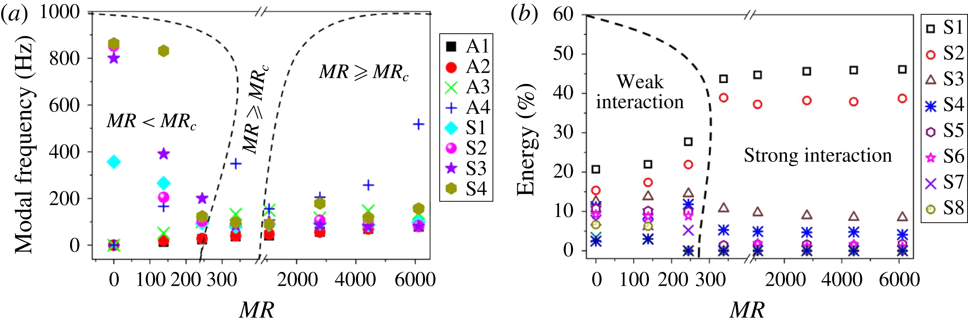
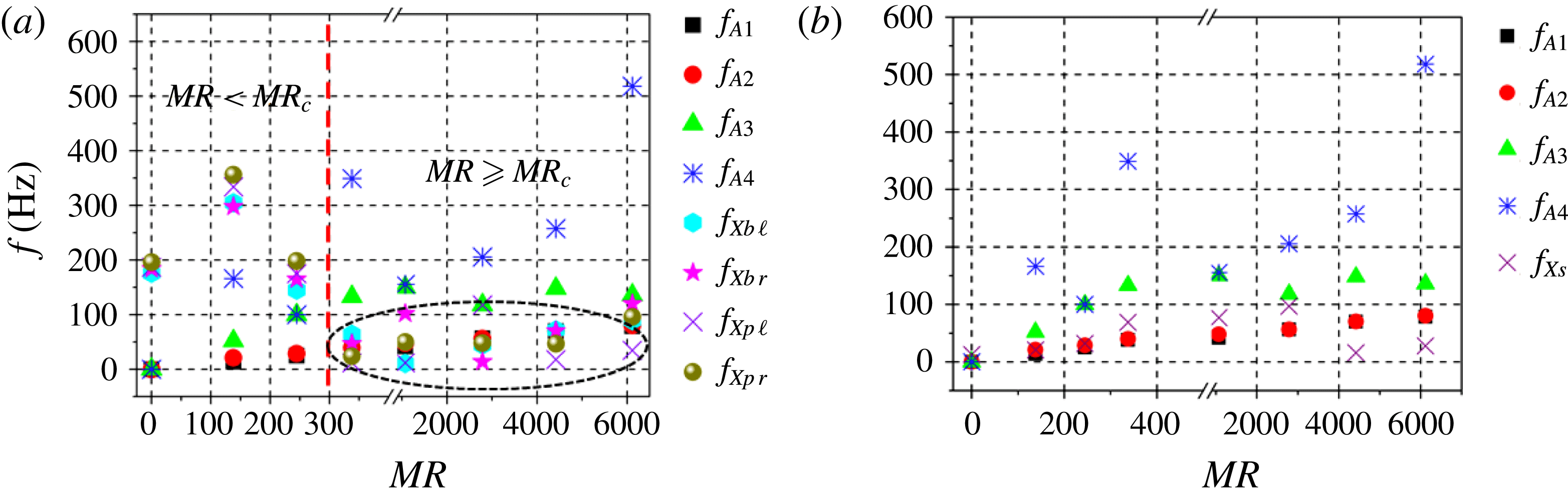
The most unstable frequency is calculated experimentally from the temporal signature of the POD modes following a similar procedure to that used in the air phase analysis. Here, the interaction between air (A) and spray (S) modes is shown by superimposing the peak frequencies of liquid and gas phase spatial eigenmodes. It can be seen that for low (
 $MR<300$
), significant mismatch exists between the modal frequencies. This implies that the spray structure is not affected significantly by the swirling air flow field (figures 8–10). In fact, for low MR values, the gas (A) and liquid (S) phase frequency values differ by several orders of magnitude (see the section labelled as
 $MR<MR_{c}$
in figure 10
a). The weak gas–liquid coupling effects in these conditions induce surface tension (‘
 $\unicode[STIX]{x1D70E}$
’) driven instabilities on the liquid surface. Further, the instability waves driven by surface tension are shown to be smaller in wavelength compared with the waves induced by gas phase (Lasheras & Hopfinger Reference Lasheras and Hopfinger2000) momentum transfer. In addition, the perturbations induced by the air phase eddies may result in low-frequency (and low-amplitude) oscillations of the liquid sheet but do not contribute towards the global deformations of the spray structures.
However, beyond
 $MR\geqslant 338$
, the modal frequencies are almost identical (particularly for modes 1 and 2). In fact, the frequency responses of the spray modes (modes 1–2) strongly resemble the air flow counterparts, indicating strong momentum coupling (figure 10
a).
(a) Comparison between air and spray modal frequencies obtained from the POD PSD (A – air modes, S – spray modes); (b) combined air and liquid phase energy contribution.

It is interesting to note that even though momentum coupling is established for higher MR values, only the first two modal frequencies (A1 and A2) of the gas phase are identical with their spray counterparts (S1, S2) (figure 10 a; slight deviations are observed between the helical modes (A3) and mode 3 of the liquid phase (S3)). In addition, the instability induced by gas phase vortex shedding (A4) is completely different from the liquid phase eigenmode S4. Similarly to the air phase, the cumulative TKE distribution for the liquid phase shows higher contributions from modes S1 and S2.
This establishes that the primary cause of interaction between the swirling air flow and the liquid sheet is via KH modes (A1 and A2). Hereafter, the modal frequencies of the air phase (only A1 and A2) are represented as ‘
 $f_{KH}$
’. However, the aforementioned observations are less significant for
 $MR\leqslant 245$
(figure 9
a–c) due to insufficient momentum coupling. Hence, the flow condition
 $MR\geqslant 338$
is identified as the critical/transition parameter (
 $MR_{c}$
).
As a first-order estimate (figures 8–10), the temporal frequency and TKE distribution indicate energy transfer between the large-scale coherent structures of the swirling field and the liquid sheet over a range of MR. However, wavelength information is needed to elucidate the details of the disturbances imposed by the flow. Hence, linear stability analysis (LSA) is carried out to estimate the wavelength and growth of the imposed disturbances.
5.3 Transition to the strong-interaction zone
This section tries to elaborate on the mechanisms responsible for the variations observed in the global structure of the spray at different MR values (air flow rates,
 $Re_{g}$
). In coaxial flows with large velocity ratios (i.e. higher MR between inner and outer streams), previous studies found that increase in the outer flow velocity beyond certain critical limits lead to partial/complete entrainment of inner fluid into the outer stream. This condition is referred to as the transition zone (Hussain & Zedan Reference Hussain and Zedan1978; Rehab, Villermaux & Hopfinger Reference Rehab, Villermaux and Hopfinger1997; Schumaker & Driscoll Reference Schumaker and Driscoll2012). Furthermore, in these transition conditions, the dynamics associated with the inner fluid (i.e. low-velocity fluid) is completely controlled by the outer stream (Villermaux & Hopfinger Reference Villermaux and Hopfinger1994). However, the behaviour of a liquid sheet in such a high-MR condition has not been analysed in detail to date to the best of our knowledge.
To explain this, we first implemented the edge detection technique on instantaneous spray images to evaluate the variation/displacement of the spray profile at different levels of the MR.
The end point of the profile at
 $MR=0$
is marked as
 $P0$
. The displacement of the sheet from
 $P0$
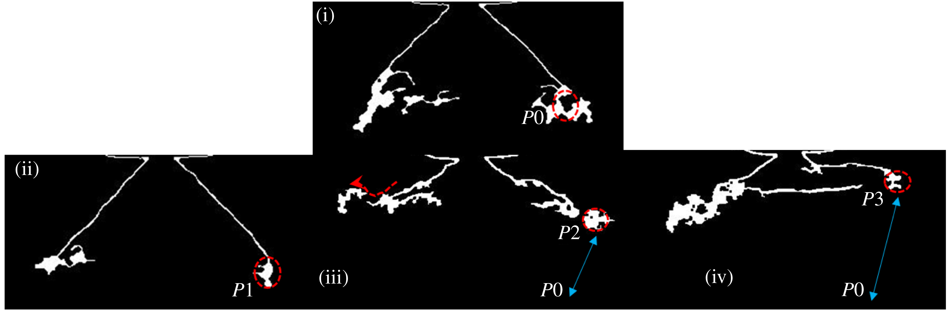
for different MR values is depicted in figure 11. It implies that the spray profile is shifted upwards (
 $P2$
and
 $P3$
) at higher MR values (see figure 11iii & iv). On the other hand, at low MR values, the displacement from
 $P0$
is not significant (shown as
 $P1$
in figure 11ii). Another interesting point to notice is that the shifted profile gets stretched in the radial direction. At the edge, the profile assumes the shape of a scoop. In general, two events are observed at higher MR values (
 $MR>338$
); the first is an upward shift of the spray profile and the second is flapping of the liquid sheet (formation of a scoop).
Schematic showing the displacement in the spray profile end point at different levels of the MR: (i)
 $MR=0$
, (ii)
 $MR=245$
, (iii)
 $MR=338$
, (iv)
 $MR=6100$
.

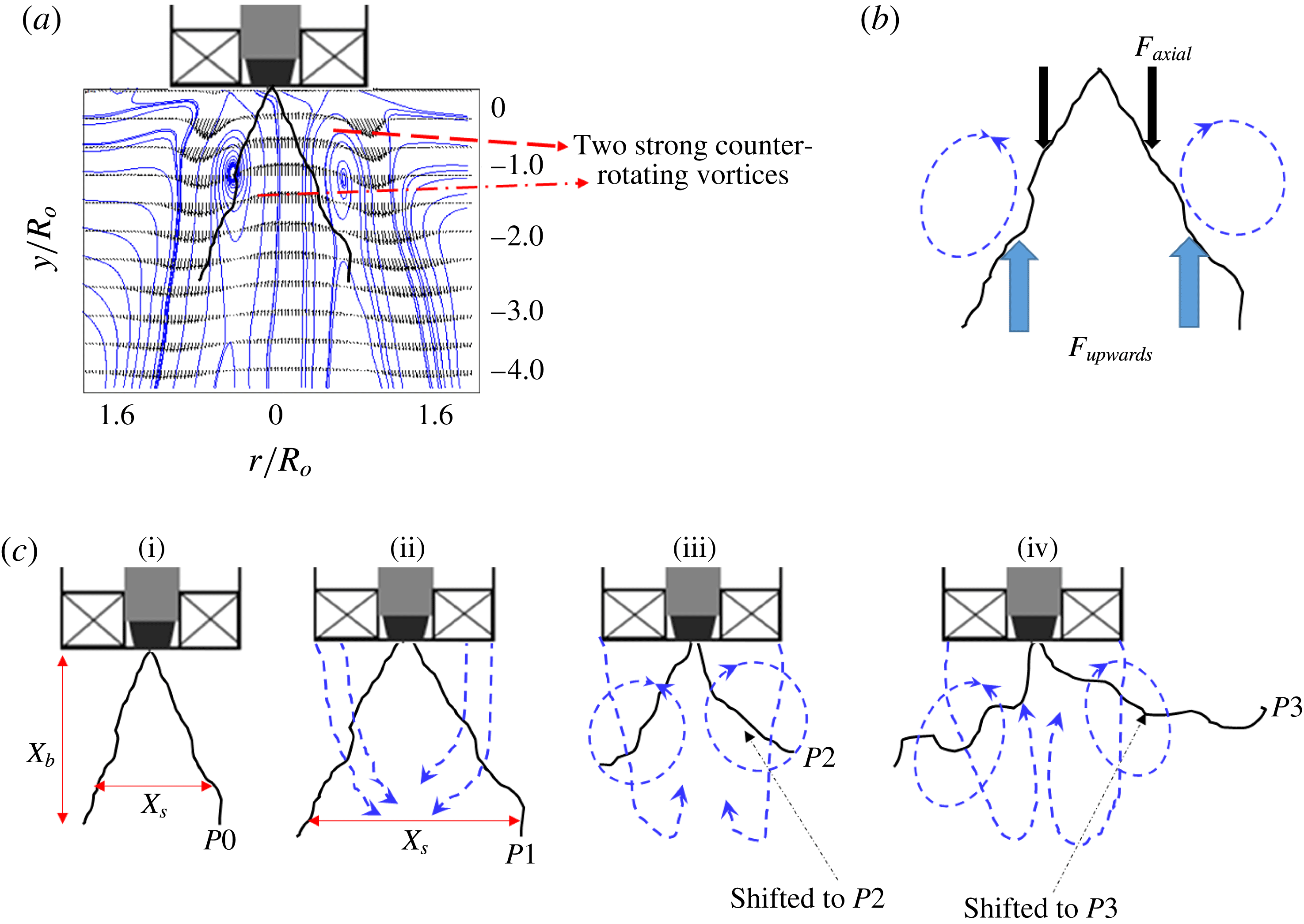
5.4 Recirculation induced profile shift (first event)
Based on the observations made from figure 11, we propose a notional diagram by superimposing the spray image with the air flow field, as shown in figure 12(a). Although both fluid streams move in the same direction, the upward shift of the spray may be due to flow recirculation of the gas phase. Recirculation is present even in normal coaxial jets at very high MR values. Hence, most of the previous entrainment models are formulated based on the ratio of recirculated mass (Rehab et al. Reference Rehab, Villermaux and Hopfinger1997). However, swirl flows naturally exhibit strong recirculation because of the vortex breakdown mechanism. Hence, we propose a simple entrainment model, which is based on the strength of inherent recirculation discussed earlier in the air flow characterization section.
(a) Spray superimposed with the time-averaged air flow streamlines; (b) forcefree body diagram; (c) schematic of the transition observed in the spray structure: (i)
 $MR=0$
; (ii)
 $MR=138$
; (iii)
 $MR=338$
; (iv)
 $MR=6100$
.

The upshift of the spray profile is accomplished by a balance between the upward lift force (
 $F_{up}$
) induced by the recirculated flow and the net axial force (
 $F_{axial}$
) acting on the liquid sheet (figure 12
b). The forces
 $F_{up}$
and
 $F_{axial}$
are expected to be of the order of
 $$\begin{eqnarray}\displaystyle & F_{up}\sim \unicode[STIX]{x1D70C}_{a}Q_{R}U_{R}, & \displaystyle\end{eqnarray}$$
 $$\begin{eqnarray}\displaystyle & F_{axial}\sim \unicode[STIX]{x1D70C}_{l}Q_{l}U_{rel}, & \displaystyle\end{eqnarray}$$
 $$\begin{eqnarray}\displaystyle & \displaystyle \unicode[STIX]{x1D6FE}=\frac{F_{up}}{F_{axial}}, & \displaystyle\end{eqnarray}$$
where
 $Q_{R}$
is the recirculated air flow rate (approximately half of the total mass flow rate is considered),
 $Q_{l}$
is the liquid flow rate through the simplex nozzle,
 $U_{R}$
is the time-averaged recirculation velocity and
 $U_{rel}$
is the relative velocity between the liquid sheet and the air flow (
 $U_{rel}\sim (U_{o}-U_{l})$
). For
 $0<MR\leqslant 245$
, the order of
 $\unicode[STIX]{x1D6FE}$
is almost unity (
 $O(\unicode[STIX]{x1D6FE})\sim 1$
), while
 $\unicode[STIX]{x1D6FE}\gg 1$
for higher MR values (
 $338\leqslant MR\leqslant 6100$
).
The above argument is made on a simple force balance model, by incorporating the values obtained from PIV and the liquid sheet axial velocity (based on mass balance). However, even the POD results also confirm the existence of strong recirculation at
 $MR\geqslant 338$
(see figure 9
d mode 1 and movie 3). In addition to upward axial force, the central recirculation shown by the
 $-\unicode[STIX]{x1D714}_{z}$
region in the air phase also imposes radial force on the liquid sheet.
In all experimental data (figures 8, 12
c, movie 4), it has been observed that, irrespective of the MR, very close to the nozzle, the liquid sheet remains intact in length (
 $X_{b}$
). To account for this effect, the dynamic pressure ratio
 $(\unicode[STIX]{x1D713})$
between the two fluids is calculated. Usually,
 $\unicode[STIX]{x1D713}$
is expressed as follows:
 $$\begin{eqnarray}\unicode[STIX]{x1D713}\sim \frac{\unicode[STIX]{x1D70C}_{a}|U_{g}^{2}|}{\unicode[STIX]{x1D70C}_{l}|U_{l}^{2}|}.\end{eqnarray}$$
The values of
 $U_{g}$
and
 $U_{l}$
are taken from the time-averaged PIV vector plots (i.e.
 $|U_{g}^{2}|$
,
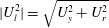 $|U_{l}^{2}|=\sqrt{U_{y}^{2}+U_{r}^{2}}$
). The calculations are made at three different positions (
 $0<y/R_{o}\leqslant 2$
) along the longitudinal axis.
In the near field,
 $y/R_{o}\leqslant 0.5$
, for all values of the MR, the value of
 $\unicode[STIX]{x1D713}$
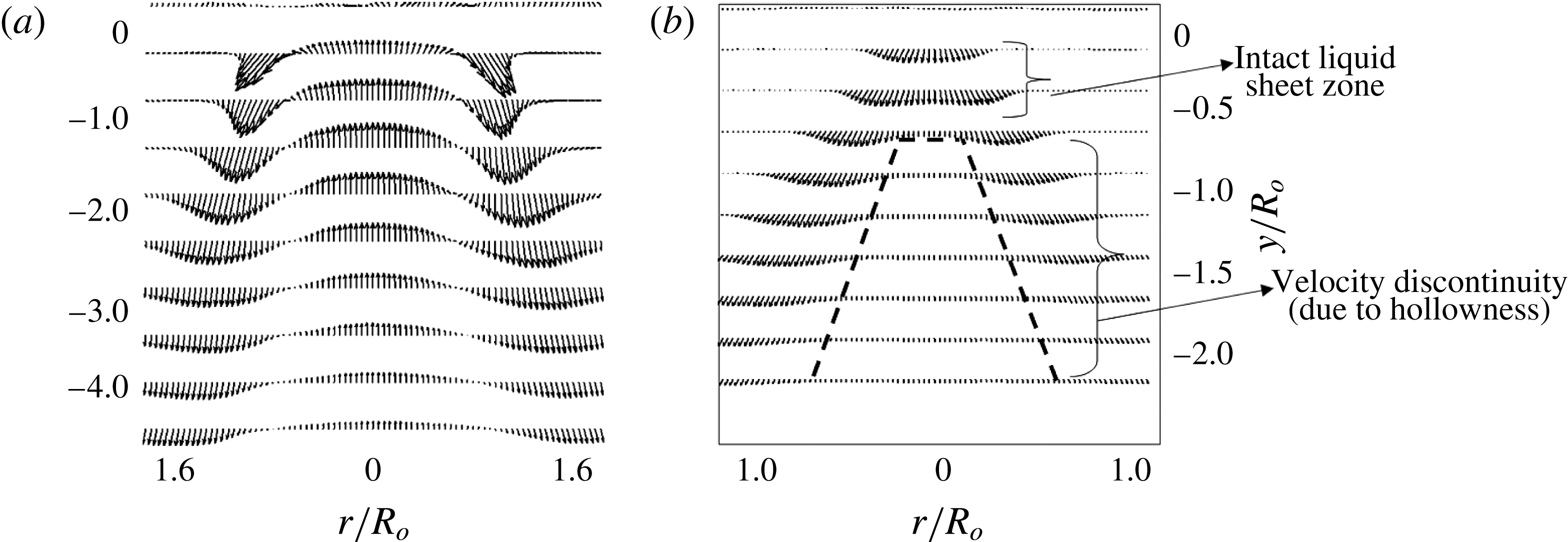
is found to be less than 1. In this region, the liquid exists like a thin sheet without any discontinuity on its surface (i.e. no discontinuity in velocity along the radius
 $0.4<r/R_{o}<0.4$
; see figure 13
b). Particularly at low values of MR,
 $\unicode[STIX]{x1D713}$
is of the order of
 $\ll 1$
, due to the fact that the velocity gradient across the two fluid streams
 $(\unicode[STIX]{x0394}U=U_{g}-U_{l})$
is lower, whereas in
 $0.5\leqslant y/R_{o}\leqslant 4$
, noticeable changes happen to
 $\unicode[STIX]{x1D713}$
at different values of the MR. Even in this region, for
 $0<MR\leqslant 245$
, the value of
 $\unicode[STIX]{x1D713}$
is less than 1
 $(\unicode[STIX]{x1D713}\approx 0.3)$
. This will create a pressure deficit along the nozzle axis and cause the outer air stream to be entrained and convected along the streamwise direction (see figure 12
cii). This event will cause the spray to expand along the radial axis with resultant alteration in the spread scale
 $X_{\boldsymbol{s}}$
(spray spread). However, for
 $338\leqslant MR\leqslant 6100$
, the magnitude of
 $\unicode[STIX]{x1D713}$
starts to approach unity (
 $\unicode[STIX]{x1D713}\approx 1$
at
 $MR=338$
), and reaches
 $\unicode[STIX]{x1D713}\approx 8$
for
 $MR=6100$
. This causes the outer air flow to assume the dominant role.
Time-averaged velocity vector field obtained from PIV. (a) Air flow field; (b) spray (without any coflowing outer air stream).

5.5 Flapping of the liquid sheet (second event)
Flapping of the liquid sheet is observed for
 $MR\geqslant MR_{c}$
because at the critical momentum ratio (
 $MR_{c}$
), formation of flow recirculation forces the liquid sheet to shift upwards and be positioned within the two strong counter-rotating vortex zones marked by
 $-1\leqslant r/R_{o}\leqslant 0.4$
and
 $-1\leqslant r/R_{o}\leqslant 1$
, as shown in figure 12(b) (also see movie 4). The boundaries of the these vortices are well established in the swirl flow literature (Anacleto et al.
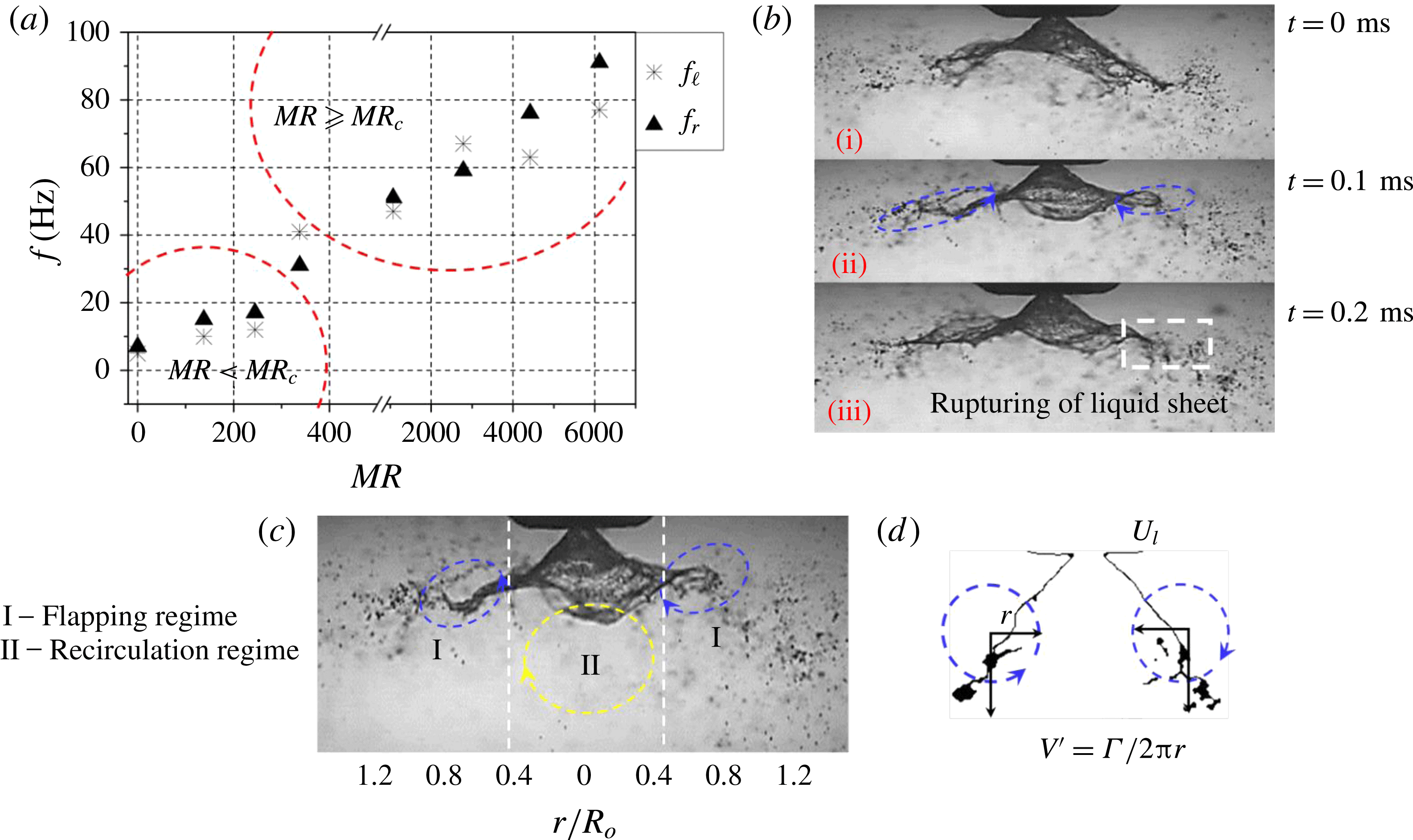
Reference Anacleto, Fernandes, Heitor and Shtork2002; Syred Reference Syred2006) as well as in this paper. The disturbances imposed by KH waves at the liquid–gas interface grow spatially (downstream) and result in flapping of the liquid sheet. Subsequently, the flapping results in periodic ejection of droplets at the edge of the liquid sheet (see the region marked with a white dotted line in figure 15
b).
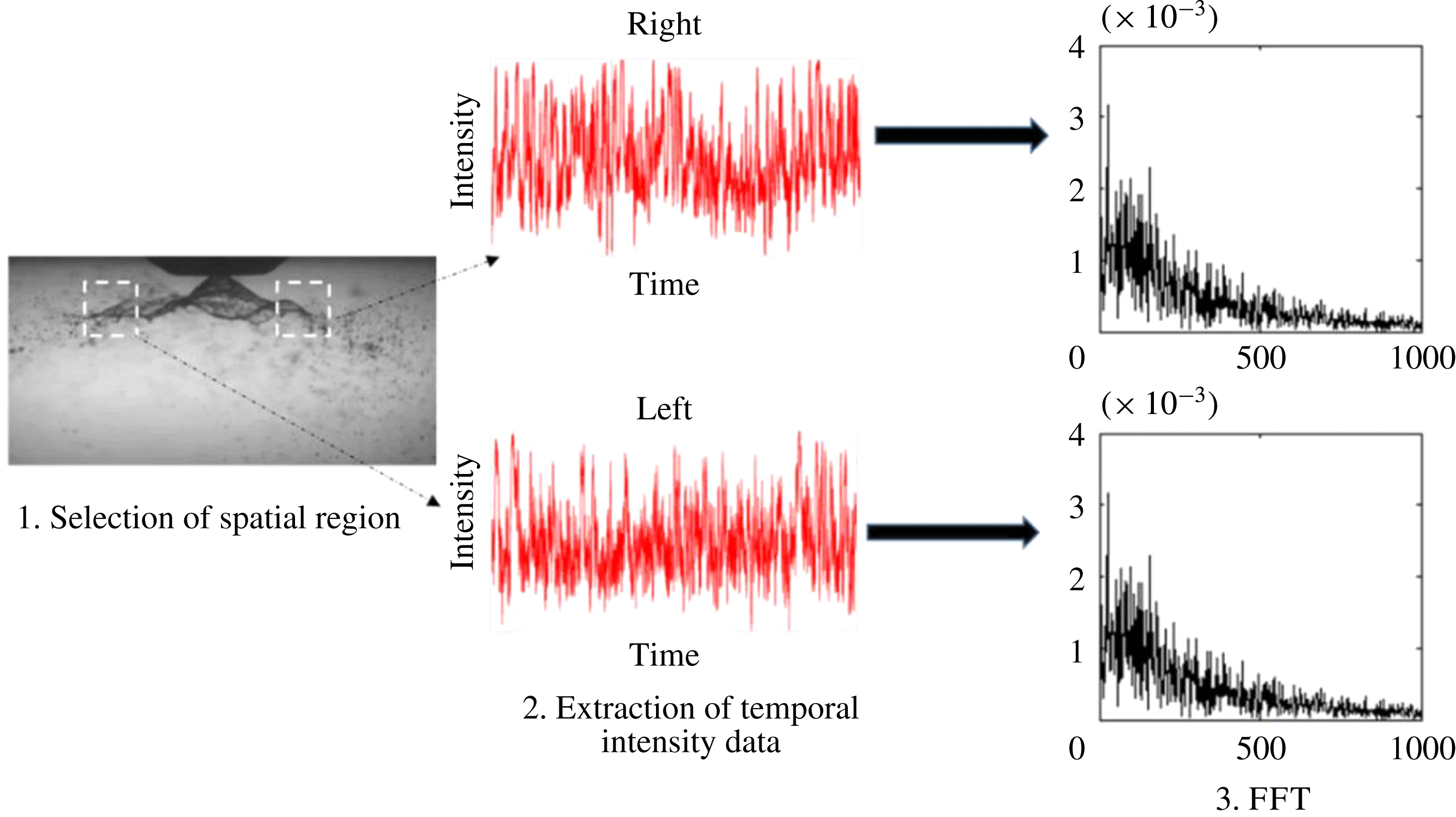
The intensity of flapping is characterized based on its frequency, which is performed by implementing a fast Fourier transform (FFT) on the temporal variation of intensity at a particular spatial location on the spray edge (figure 14). The processing involves identification of an optimal region, which corresponds to flapping (drawing a square box around that region; step 2), extraction of the average intensity in that region (step 2) and implementing FFT (step 3) to extract the dominant frequency (figure 14). This was carried out on both sides of the spray longitudinal axis (i.e. left and right). This calculation does not account for disturbances/undulations imposed (
 $\unicode[STIX]{x1D706}$
) on the surface of the liquid sheet. This will only estimate the intermittency, i.e. the number of times that the liquid sheet/edge appears in the spatial window (shown by white dotted lines in figure 14).
The steps involved in extracting flapping frequency information from the instantaneous spray images.

The spatially averaged frequencies obtained from the instantaneous spray images reveal a significant increase in flapping at
 $MR\geqslant MR_{c}$
along with slight deviation in frequency values between the left and right sides (see figure 15
a). However, the shedding induced by the PVC (identified as mode 4 in POD) carries very low energy. As a result, the flapping frequency is not synchronized with the shedding mode of the air flow field, whereas the flapping of the liquid sheet is well synchronized with the peak frequencies of air phase KH instability modes, i.e. A1 and A2 (
 $f_{l,r}\approx f_{KH}$
). Furthermore, the time scales of one complete flapping cycle
 $(\unicode[STIX]{x1D70F}_{f})$
and the droplet ejection rate
 $(\emptyset )$
are found to scale with the vortex shedding time
 $(\unicode[STIX]{x1D70F}_{f}\approx \unicode[STIX]{x1D70F}_{s})$
in that region. The reason will be explained in more detail in § 6. In the region away from the vortex core centre (
 $V_{cc}$
), the rotating eddies impose an aerodynamic force
 $F_{c}$
on the liquid sheet, where
 $(F_{c}=\unicode[STIX]{x1D70C}_{a}(V^{\prime 2}))$
; here,
 $V^{\prime }$
is the circulation induced velocity,
 $V^{\prime }=\unicode[STIX]{x1D6E4}/2\unicode[STIX]{x03C0}r$
;
 $\unicode[STIX]{x1D6E4}$
is the circulation strength. Slight deviation is observed in the calculated circulation strength between the left and right side eddies, which results in dissimilar flapping frequency values (see figure 15
a) at the left (
 $f_{l}$
) and right sides (
 $f_{r}$
). The liquid sheet starts to interact with counter-rotating eddies if the induced velocity
 $V^{\prime }$
is sufficiently larger than the liquid sheet velocity (
 $U_{l}$
). As explained earlier, the radius
 $r$
of the vortex remains unchanged across all flow conditions. Hence, the droplet ejection rate
 $(\emptyset )$
is a function of the circulation intensity of the two vortices
 $\unicode[STIX]{x1D719}=f(\unicode[STIX]{x1D6E4})$
.
(a) Time-averaged flapping frequency in the flapping region; (b) interaction of the liquid sheet with two opposite counter-rotating vortices and rupturing of the liquid sheet at the edge; (c) liquid sheet evolution in the spatial regime; (d) counter-rotating vortices induced velocity (
 $V^{\prime }$
) in region I.

During intense flapping
 $(f_{l,r}\approx 60~\text{Hz})$
, the liquid sheet at the edge is completely ruptured and leads to the formation of clusters of droplets (figure 15
b).
The global variations can be summarized as follows:
 $0\leqslant MR\leqslant 245\rightarrow \text{weak\text{-}interaction zone}$
(see movie 2);
 $MR\approx 338\rightarrow \text{transition/critical zone}$
(see movie 3);
 $338\leqslant MR\leqslant 6100\rightarrow \text{strong\text{-}interaction zone}$
(see movie 4).
Therefore, the flow condition associated with
 $MR\approx 338$
is taken as the critical value (
 $MR_{c}$
).
Furthermore, two main regimes are identified in the spatial region, as shown in figure 15(c),
 $$\begin{eqnarray}\displaystyle & \displaystyle -0.4\leqslant \frac{r}{R_{o}}\leqslant 0.4\rightarrow \mathit{recirculation~region~(I)}, & \displaystyle\end{eqnarray}$$
 $$\begin{eqnarray}\displaystyle & \displaystyle \left.\begin{array}{@{}c@{}}-1\leqslant {\displaystyle \frac{r}{R_{o}}}\leqslant -0.4\\ 0.4\leqslant {\displaystyle \frac{r}{R_{o}}}\leqslant 1\end{array}\right\}\rightarrow \mathit{flapping~region~(II)}. & \displaystyle\end{eqnarray}$$
6 Linear stability analysis
To this end, we discuss the spatial variations and transitions observed in the flow field as a function of the MR. In this section, we perform an LSA to determine the length scales associated with the most unstable wavelength, which is likely to control the atomization pathways. In addition, comparison is made between experimental (derived from POD) and theoretical (LSA) frequency values.
6.1 Problem formulation
The instability of the mixing layer formed between coaxial shear flows with identical or different densities has been explained by several researchers (Lin Reference Lin1966; Brown & Roshko Reference Brown and Roshko1974; Monkewitz & Huerre Reference Monkewitz and Huerre1982; Metcalfe et al.
Reference Metcalfe, Orszag, Brachet, Menon and Riley1987). In particular, in situations like coaxial atomization where a two-phase mixing layer exists, studies (Juniper & Candel Reference Juniper and Candel2003; Fuster et al.
Reference Fuster, Matas, Marty, Popinet, Hoepffner, Cartellier and Zaleski2013) reveal that for a high dynamic pressure ratio
 $\unicode[STIX]{x1D713}$
, instability is mostly controlled by air flow. Experiments carried out in a two-phase mixing layer by Raynal et al. (Reference Raynal, Villermaux, Lasheras and Hopfinger1997) and Matas, Marty & Cartellier (Reference Matas, Marty and Cartellier2011) showed that the formation of a vorticity layer and its thickness
 $(\unicode[STIX]{x1D6FF}_{g})$
around the liquid flow determine the primary wavelength of the most unstable mode. They also showed that the length scales of such wavelengths are much larger than the vorticity thickness.
In this study, we propose a linear stability model incorporating the vorticity thickness (i.e. continuous velocity profile across the interface) (see, e.g., Rayleigh 1880; Boeck & Zaleski Reference Boeck and Zaleski2005 and figure 16). Here, LSA is only proposed to supplement/corroborate the experimental analyses (like those obtained from POD) as a first-order estimation of the most unstable wavelength especially for
 $MR\geqslant MR_{c}$
. The combined spatio-temporal LSA is necessary to predict the transition from convective to absolute. However, to perform spatial-stability analysis it is mandatory to satisfy the Gaster criterion (Gaster Reference Gaster1962),
 $\{(\unicode[STIX]{x1D714}_{i}/f)\ll 1\}$
. However, in the present study, for all of the test cases (particularly for
 $MR>MR_{c}$
), the Gaster criterion is not satisfied. This may be due to large values of the MR (as shown in Matas et al. (Reference Matas, Marty and Cartellier2011)). Hence, we perform only temporal LSA to predict the growth rate for the imposed disturbance as a first-order estimate only.
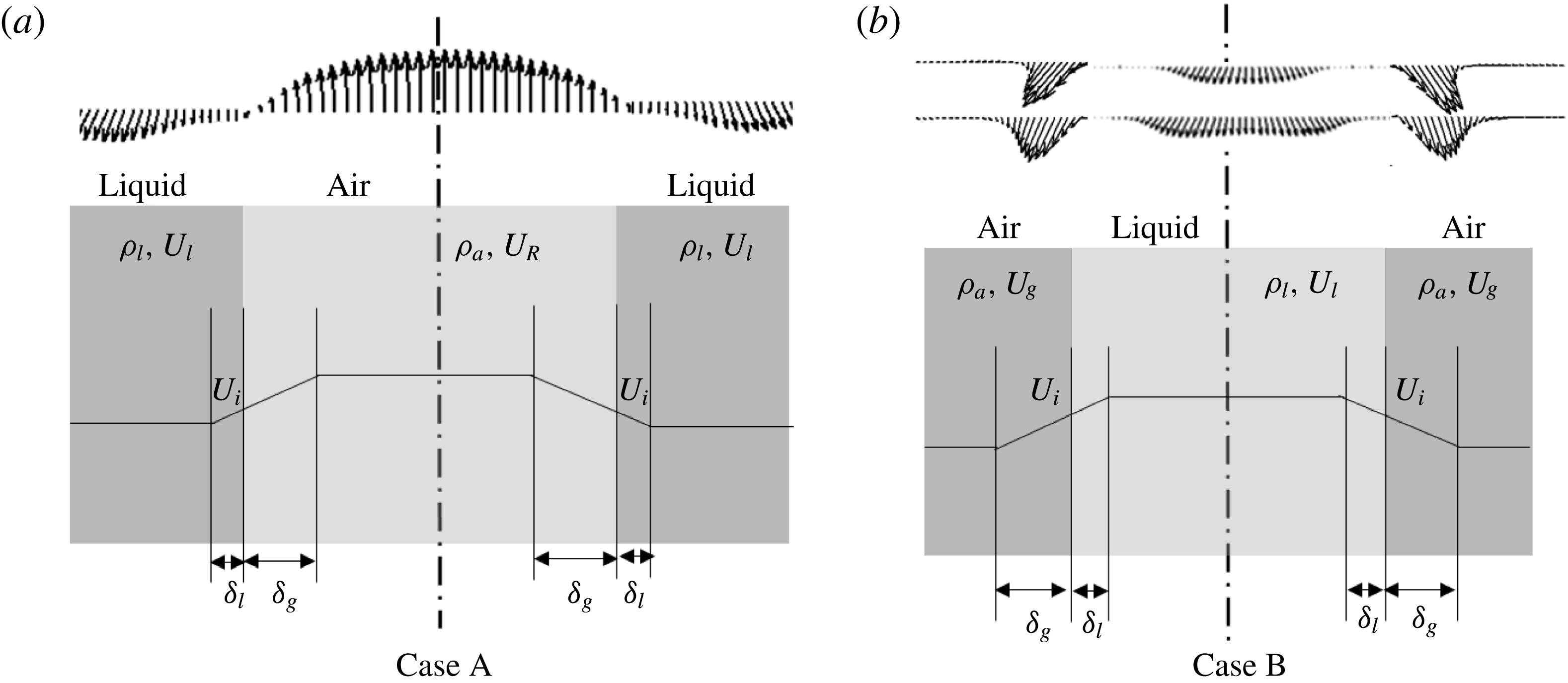
Approximated velocity profiles with gas and liquid layer thickness. (a) Case A, superimposition of the recirculated air velocity profile with the liquid; (b) case B, bulk-averaged liquid and air flow exit velocity profiles. Here,
 $U_{i}$
is the interfacial velocity.

Since swirl streams exhibit flow in both the streamwise and opposite directions (i.e. recirculated flow), we consider two velocity profile models (figure 16). The first one has recirculated flow forming an interface with the liquid flow (case A). In case B, the bulk-averaged air and liquid flow velocity profile is considered. Some previous studies (Marmottant & Villermaux Reference Marmottant and Villermaux2004; Ben Rayana Reference Ben Rayana2007) have suggested that
 $\unicode[STIX]{x1D6FF}_{g}\gg \unicode[STIX]{x1D6FF}_{l}$
; so in both cases we neglect
 $\unicode[STIX]{x1D6FF}_{l}$
.
The gas vorticity layer thickness is expressed as a function of the gas Reynolds number
 $(Re_{g})$
(Raynal et al.
Reference Raynal, Villermaux, Lasheras and Hopfinger1997),
 $$\begin{eqnarray}\unicode[STIX]{x1D6FF}_{g}\approx 8.5D_{eff}\sqrt{Re_{g}}.\end{eqnarray}$$
Here,
 $D_{eff}$
is the effective air flow path diameter across the swirler, which is evaluated from (2.3).
To calculate the most unstable wavelength, the dispersion relation, which accounts for KH instability arising at the interface of the two parallel streams, is used (see, e.g., Chandrasekhar Reference Chandrasekhar2013),
 $$\begin{eqnarray}\text{e}^{-2\unicode[STIX]{x1D712}}=\left[1-2\left(\unicode[STIX]{x1D71B}+\frac{r}{r-1}\right)\right]\ast \left\{\frac{1+\left({\displaystyle \frac{\unicode[STIX]{x1D70C}_{l}}{\unicode[STIX]{x1D70C}_{a}}}+1\right)\left(\unicode[STIX]{x1D71B}+{\displaystyle \frac{\unicode[STIX]{x1D712}}{r-1}}\right)}{1+\left({\displaystyle \frac{\unicode[STIX]{x1D70C}_{l}}{\unicode[STIX]{x1D70C}_{a}}}-1\right)\left(\unicode[STIX]{x1D71B}+{\displaystyle \frac{\unicode[STIX]{x1D712}}{r-1}}\right)}\right\},\end{eqnarray}$$
where
 $r=U_{R}/U_{l}$
(case A),
 $r=U_{g}/U_{l}$
(case B),
 $\unicode[STIX]{x1D712}=K\unicode[STIX]{x1D6FF}_{g}$
,
 $K$
is the wavenumber (
 $2\unicode[STIX]{x03C0}/\unicode[STIX]{x1D706}$
),
 $\unicode[STIX]{x1D71B}=\unicode[STIX]{x1D714}\unicode[STIX]{x1D6FF}_{g}/(U_{o}-U_{l})$
and
 $\unicode[STIX]{x1D714}$
is the growth rate
 $(\text{s}^{-1})$
. The solution of (5.3) is complex
 $(\unicode[STIX]{x1D71B}=\unicode[STIX]{x1D71B}_{r}+\text{i}\unicode[STIX]{x1D71B}_{i})$
. Here, only the term corresponding to the growth rate/damping coefficient is considered (i.e.
 $\text{i}\unicode[STIX]{x1D71B}_{i}$
).
From Betchov & Szewczyk (Reference Betchov and Szewczyk1963), the damping role of the viscosity in the stability of two parallel flow streams can be neglected, if
 $Re_{\unicode[STIX]{x1D6FF}}>100$
,
 $$\begin{eqnarray}Re_{\unicode[STIX]{x1D6FF}}=\frac{U_{g}\unicode[STIX]{x1D6FF}_{g}}{\unicode[STIX]{x1D710}_{g}},\end{eqnarray}$$
where
 $U_{g}$
is the gas velocity,
 $\unicode[STIX]{x1D6FF}_{g}$
is the gas shear layer thickness and
 $\unicode[STIX]{x1D710}_{g}$
is the kinematic viscosity of gas.
In the present experiments, for all of the test cases, the value of
 $Re_{\unicode[STIX]{x1D6FF}}$
is greater than 100. Particularly for higher air flow rates (
 $2785\leqslant MR\leqslant 6100$
), the values are much greater than 100
 $(Re_{\unicode[STIX]{x1D6FF}}\gg 100)$
. Hence, the damping effect due to viscosity is not considered in (6.2). However, damping may play a role for
 $0\leqslant MR\leqslant 245$
.
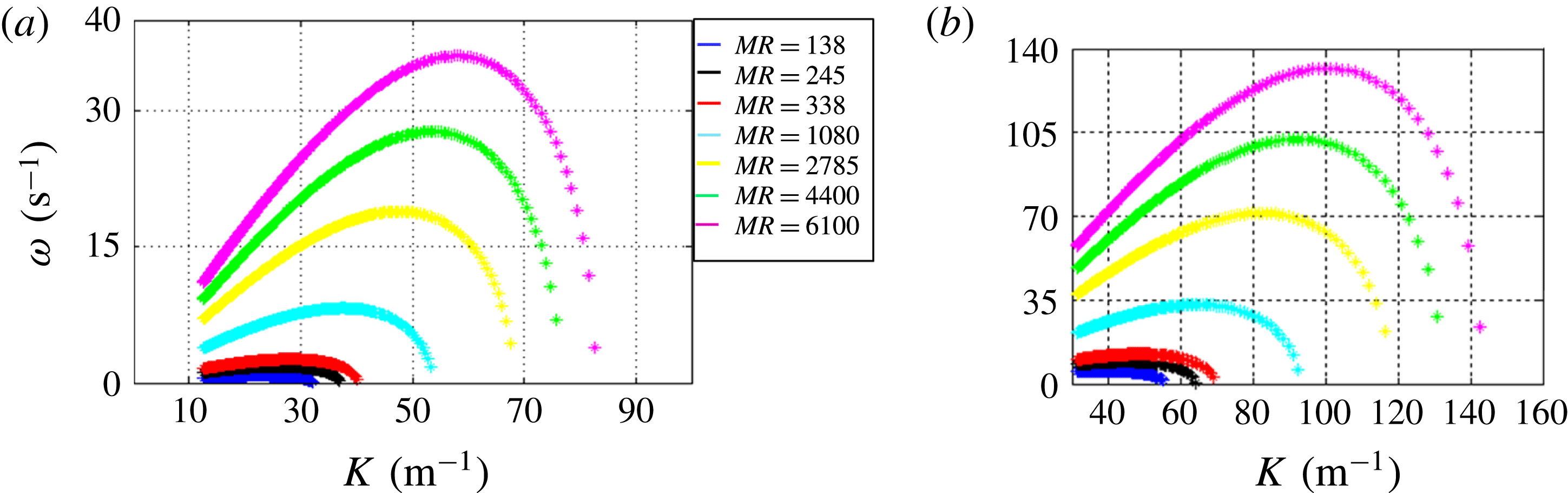
Equation (6.2) is solved for different
 $\unicode[STIX]{x1D706}$
values (i.e.
 $K$
), and corresponding growth rates are plotted in figure 17. The value corresponding to
 $\unicode[STIX]{x1D714}_{max}$
is equated with
 $K_{max}$
to obtain the most unstable wavelength
 $(\unicode[STIX]{x1D706}_{max})$
. In addition, the cutoff wavelength
 $(\unicode[STIX]{x1D706}_{c})$
is calculated from
 $K_{c}$
.
Dispersion diagram showing the growth rate as a function of the wavenumber.

Further, the frequency values are calculated from the most unstable wavelength
 $(\unicode[STIX]{x1D706}_{max})$
using the relation
 $f_{t}\approx U_{i}/\unicode[STIX]{x1D706}_{max}$
, where
 $U_{i}$
is the interfacial velocity which can be evaluated based on the dynamic pressure balance across the two fluid streams (Cebeci & Bradshaw Reference Cebeci and Bradshaw1977; Dimotakis Reference Dimotakis1986),
 $$\begin{eqnarray}\unicode[STIX]{x1D70C}_{l}(\unicode[STIX]{x0394}U)_{l}^{2}=\unicode[STIX]{x1D70C}_{a}(\unicode[STIX]{x0394}U)_{g}^{2},\end{eqnarray}$$
where
 $\unicode[STIX]{x0394}U_{l}=U_{i}-U_{l}$
and
 $\unicode[STIX]{x0394}U_{g}=U_{g}-U_{i}$
; this condition will be hold only for
 $U_{i}>U_{l}$
(i.e. laminar liquid and turbulent air flows),
 $$\begin{eqnarray}U_{i}\sim \frac{\sqrt{\unicode[STIX]{x1D70C}}_{a}U_{g}+\sqrt{\unicode[STIX]{x1D70C}}_{l}U_{l}}{\sqrt{\unicode[STIX]{x1D70C}}_{a}+\sqrt{\unicode[STIX]{x1D70C}}_{l}}.\end{eqnarray}$$
6.2 Comparison with experiments
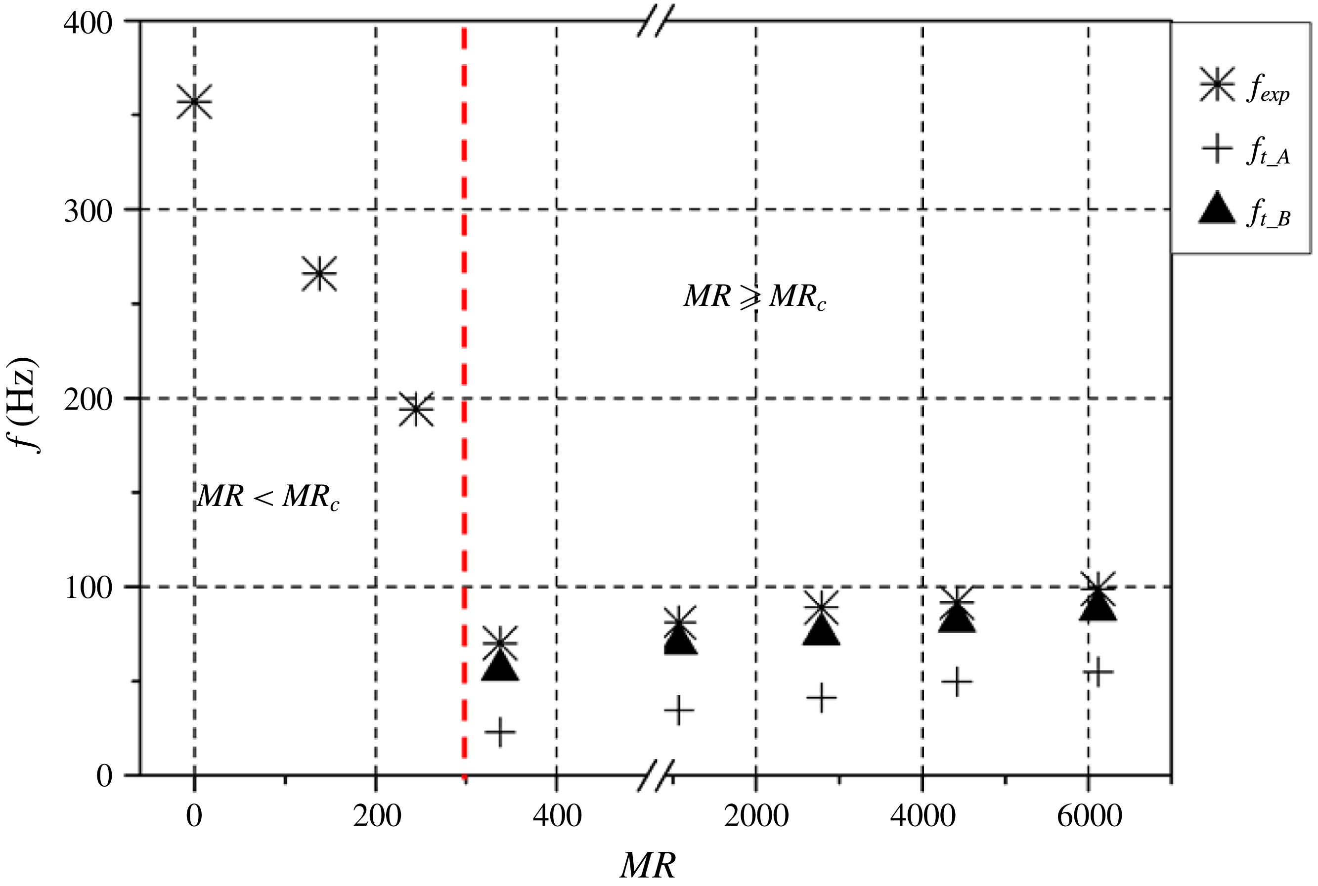
Figure 18 depicts a comparison between the theoretical and experimental frequency values evaluated from LSA and POD modes. The experimental frequencies shown in figure 18 correspond to global instability phenomena obtained from POD using the method of snapshots algorithm, which also accounts for surface undulations (
 $\unicode[STIX]{x1D706}$
). Here, the asymptotic nature of the frequency (figure 18) is due to the dominance of the liquid phase in the
 $MR<MR_{c}$
region (i.e. weak coupling of the gas phase with the liquid phase). In the liquid-dominated regime (i.e.
 $MR=0$
and
 $MR<MR_{c}$
), the surrounding ambient air imposes small-scale disturbances on the expanding liquid sheet and results in much shorter wavelengths. The occurrence of these small-scale wavelengths on the surface of the liquid sheet is well documented by Squire (Reference Squire1953), Hagerty & Shea (Reference Hagerty and Shea1955) and Dombrowski & Johns (Reference Dombrowski and Johns1963). This, in turn, results in high-frequency values compared with the
 $MR\geqslant MR_{c}$
region.
Experimental (POD KH modes) versus theoretical frequency (
 $f_{t_A,B}$
is the theoretical frequency obtained for cases A and B).

These high-frequency values do not show up in flapping (figure 15 a), where the analysis was carried out at fixed spatial location and accounts only for the spread rate of the liquid edge. Hence, the values shown in figures 15(a) and 18 are completely different.
Conversely, at high air flow rates (
 $MR\geqslant MR_{c}$
), the above short-wavelength disturbances are damped, and formation of a gas shear layer
 $(\unicode[STIX]{x1D6FF}_{g})$
results in amplification of long wavelengths. This was first reported by Raynal et al. (Reference Raynal, Villermaux, Lasheras and Hopfinger1997) and followed by Lasheras & Hopfinger (Reference Lasheras and Hopfinger2000) and Ben Rayana (Reference Ben Rayana2007). This may be the reason why frequency values are relatively lower compared with the
 $MR<MR_{c}$
region, as progressive increase in air flow tries to damp short waves and induce growth of long waves. However, in this regime (
 $MR\geqslant MR_{c}$
), wavelength (long wavelength) decreases with increasing MR, which in turn causes a relative increase in frequency. This can be visualized from the eigenmodes of the spray (S1, S2) and gas (A1, A2) phases (see figures 6
a, 9
d–h).
The theoretical frequency
 $(f_{t})$
corresponding to case B shows a better match compared with case A (from figure 17 it is observed that
 $K_{max}$
is reduced by half for the recirculated flow case). This is because in case A, the velocity magnitude corresponding to recirculation alone is considered, whereas in case B, the combined streamwise and recirculated velocity profile is used (ideally this velocity magnitude is higher than the recirculated flow velocity alone). Furthermore, the combined velocity shear induced by both velocity profiles is shown as a high-shear zone. Interestingly, it has already been shown that
 $f_{s1,s2}$
scales reasonably with the air phase eigenmodes (i.e.
 $f_{s1,s2}\approx f_{A1,A2}$
).
The above arguments are true only when the air flow rate is sufficiently high and the role played by the surface tension of the liquid is negligible (i.e.
 $MR\geqslant MR_{c}$
). The simple LSA proposed in this study (based on
 $\unicode[STIX]{x1D6FF}_{g}$
) will yield reasonable results only when the gas KH waves are superimposed on the liquid phase (strong coupling). This is the reason why the frequency values in the
 $MR<MR_{c}$
region do not scale with the theoretical frequency (the effect of the gas flow field is rather weak).
Hence, the vorticity thickness at
 $MR\approx MR_{c}$
is considered as the critical thickness
 $(\unicode[STIX]{x1D6FF}_{gc})$
. From the above arguments, the relationship among flow parameters, the most unstable wavelength and its growth rate can be written as
 $$\begin{eqnarray}\displaystyle & \displaystyle \unicode[STIX]{x1D706}_{max}\approx \unicode[STIX]{x1D6FF}_{g}\sqrt{\frac{\unicode[STIX]{x1D70C}_{l}}{\unicode[STIX]{x1D70C}_{a}}}\quad (\text{for }MR\geqslant MR_{c}), & \displaystyle\end{eqnarray}$$
 $$\begin{eqnarray}\displaystyle & \displaystyle (\unicode[STIX]{x1D714}_{i})_{max}=\sqrt{\frac{\unicode[STIX]{x1D70C}_{a}}{\unicode[STIX]{x1D70C}_{l}}}\frac{(U_{a}-U_{i})}{\unicode[STIX]{x1D6FF}_{g}}. & \displaystyle\end{eqnarray}$$
7 Breakup dynamics and global length scales
This section illustrates the mechanisms and dynamics associated with liquid sheet breakup at different levels of MR. In addition to the MR, another relevant non-dimensional parameter, called the Weber number, is also used,
 $$\begin{eqnarray}We_{t}=\frac{\unicode[STIX]{x1D70C}_{a}(U_{a}-U_{l})t_{f}}{\unicode[STIX]{x1D70E}},\quad We_{\unicode[STIX]{x1D6FF}}=\frac{\unicode[STIX]{x1D70C}_{a}(U_{a}-U_{l})\unicode[STIX]{x1D6FF}_{g}}{\unicode[STIX]{x1D70E}},\end{eqnarray}$$
where
 $t_{f}$
is the liquid film thickness and
 $\unicode[STIX]{x1D70E}$
is the surface tension.
In addition to
 $We_{t}$
and
 $We_{\unicode[STIX]{x1D6FF}}$
, the Weber number is also defined in the flapping region based on circulation strength
 $(\unicode[STIX]{x1D6E4})$
, where
 $r$
is the vortex core radius,
 $$\begin{eqnarray}We_{\unicode[STIX]{x1D6E4}}=\frac{\unicode[STIX]{x1D70C}_{a}\left({\displaystyle \frac{\unicode[STIX]{x1D6E4}}{2\unicode[STIX]{x03C0}r}}\right)^{2}t_{f}}{\unicode[STIX]{x1D70E}}.\end{eqnarray}$$
7.1 Image processing
The spray images obtained from high-speed shadowgraphy are processed to obtain the time-averaged and instantaneous breakup lengths. Actually, two types of breakup length are evaluated. One is measured from the nozzle exit to the point where the sheet shows the first signs of breakup (
 $X_{b}$
). The other is based on tracking the spray edge profile
 $X_{p}$
(the detailed steps are shown in figure 19). All of the measurements are carried out on both the left (
 $X_{bl},X_{pl}$
) and right (
 $X_{br},X_{pr}$
) sides of the spray across the longitudinal axis (
 $y$
) of the nozzle.
Image processing algorithm to evaluate length scales and its characteristic frequency.

7.2 Characteristic frequency and length scale dynamics
Fast Fourier transform is implemented on the instantaneous
 $X_{b},X_{p}$
values to acquire the dynamics associated with the breakup length scales. The comparison plot for characteristic length scale frequencies (figure 20) depicts a reasonably good match with air POD modes 1 and 2
 $(f_{KH}\approx f_{Xbl},f_{Xbr},f_{Xpl},f_{Xpr})$
for
 $MR\geqslant MR_{c}$
(black circled region in figure 20). In Weber number space, this corresponds to
 $1\leqslant We_{t},We_{\unicode[STIX]{x1D6FF}}\leqslant 25$
. Therefore, the Weber number corresponding to the critical zone (i.e.
 $MR\approx MR_{c}$
) is considered as
 $We_{\unicode[STIX]{x1D6FF},C},We_{g,C}$
. Furthermore, when
 $MR\geqslant MR_{c}$
, the Weber number based on the circulation strength in the flapping region also indicates a strong aerodynamic force over the liquid sheet. Below critical MR, the Weber number is below 1, indicating that breakup is less affected by the swirling air field.
Comparison of the air modal frequency with the breakup and spread length scale characteristic frequencies
 $f_{A1,2,3,4}$
(air modal frequencies) and
 $f_{Xb}$
,
 $f_{Xp}$
(breakup length characteristic frequencies), where the subscripts
 $l,r$
represent the left and right sides of the spray.

In addition to the breakup length scale (
 $X_{b}$
), the lateral expansion of the spray (i.e. spray spread)
 $X_{s}$
is also evaluated (the procedure is shown in figure 19, step 5), and its characteristic frequency values are shown in figure 20. Even though
 $f_{KH}\approx f_{Xs}$
, at higher MR values (
 $4400\leqslant MR\leqslant 6100$
), frequency values are decreased by five times. In this condition, it is observed that the lateral expansion is saturated and the liquid sheet starts to rupture at the edges due to intense flapping (see movie 3). It is also interesting to note that, even at
 $MR<MR_{c}$
, the frequency values match with the air eigenmodes (only the first two modes), which was not observed for other events.
This is due to the fact that, even at lower MR values, lower values of
 $\unicode[STIX]{x1D713}$
cause air entrainment inside the liquid cone and result in expansion along the radial direction.
7.3 Time-averaged length scales
In most atomizers, the breakup length depends on the breakup time scale and the velocity of the liquid sheet. In coaxial atomizers, velocity values are usually scaled with the most unstable primary wavelength forming on the liquid sheet–air interface prior to breakup. Experiments carried out by Lasheras et al. (Reference Lasheras, Villermaux and Hopfinger1998) in a round liquid jet with coflowing air established that the breakup length is well correlated with the velocity difference (
 $u_{g}^{\prime }$
;
 $u_{g}^{\prime }=\unicode[STIX]{x1D6FC}(U_{g}-U_{l})$
, where
 $\unicode[STIX]{x1D6FC}=0.17$
) between the gas and liquid phases (i.e. in the two-phase mixing layer). However, in the present geometry, liquid emerges in the form of a hollow liquid cone with thickness
 $t_{f}\approx 0.2~\text{mm}$
. Park et al. (Reference Park, Huh, Li and Renksizbulut2004) showed that the breakup time associated with the liquid sheet scales with the maximum growth rate of the wave,
 $$\begin{eqnarray}X_{b}\approx t_{b}\ast \;\text{velocity}.\end{eqnarray}$$
The breakup time
 $(t_{b})$
is evaluated from the high-speed shadowgraphy images by observing the time lapse between two successive events, and the values are found to be
 $0.1\ast \{1/(\unicode[STIX]{x1D714}_{i})_{max}\}$
,
 $$\begin{eqnarray}X_{b}\approx 0.1\{1/(\unicode[STIX]{x1D714}_{i})_{max}\}\ast V.\end{eqnarray}$$
For the velocity scale (
 $V$
), previously it was shown that at high air flow rates
 $(MR\geqslant MR_{c})$
, the interface of the liquid sheet is stretched by the interfacial velocity (
 $V\approx U_{i}$
) arising from the dynamic pressure ratio balance (6.4) and (6.5),
 $$\begin{eqnarray}\displaystyle & \displaystyle X_{b}\approx 0.1\{1/(\unicode[STIX]{x1D714}_{i})_{max}\}\ast U_{i}, & \displaystyle\end{eqnarray}$$
 $$\begin{eqnarray}\displaystyle & \displaystyle X_{b}\approx 0.1\{1/(\unicode[STIX]{x1D714}_{i})_{max}\}(f_{KH}\ast \unicode[STIX]{x1D706}_{max}), & \displaystyle\end{eqnarray}$$
 $$\begin{eqnarray}\displaystyle & \displaystyle X_{b}\approx 0.1\left\{\frac{1}{\sqrt{{\displaystyle \frac{\unicode[STIX]{x1D70C}_{a}}{\unicode[STIX]{x1D70C}_{l}}}}\frac{(U_{a}-U_{i})}{\unicode[STIX]{x1D6FF}_{g}}}\right\}f_{KH}\ast \unicode[STIX]{x1D6FF}_{g}\sqrt{\frac{\unicode[STIX]{x1D70C}_{l}}{\unicode[STIX]{x1D70C}_{a}}}. & \displaystyle\end{eqnarray}$$
Figure 21 depicts the normalized breakup length comparison between experiments and theory. It is seen that the theoretical results agree well with experiments at
 $(MR\geqslant MR_{c})$
. This indicates that at higher flow rates, the length scale, which corresponds to
 $\unicode[STIX]{x1D706}_{max}$
, controls the breakup phenomena of the liquid sheet (due to
 $We_{\unicode[STIX]{x1D6FF}}\geqslant We_{\unicode[STIX]{x1D6FF},C}$
). However,
 $\unicode[STIX]{x1D706}_{max}$
does not scale with
 $X_{b}$
at low air flow rates (
 $MR<MR_{c}$
), which indicates the dominant role of surface tension.
The time-averaged breakup length normalized with the sheet thickness
 $(t_{f})$
; here,
 $X_{bt}$
is the theoretical breakup length; where the subscripts
 $l,r$
represent the left and right sides of the spray.

Illustration of the time-averaged spray spread (
 $X_{s}$
).

At very high air flow rates (
 $4400\leqslant MR\leqslant 6100$
), asymmetry is observed in the breakup length. This may be due to the chaotic/catastrophic (non-uniform) breakup of the liquid sheet (see the region shown as III in figure 21 and also refer to figure 23(i)f,g) induced by the increased circulation strength (i.e.
 $We_{\unicode[STIX]{x1D6E4}}\gg 1$
) of the counter-rotating eddies. To check this observation, the standard deviation
 $(\unicode[STIX]{x1D70E}_{Xb})$
is calculated for the instantaneous left and right side breakup lengths. It shows wider dispersion for (
 $4400\leqslant MR\leqslant 6100$
).
The time-averaged spray spread scale is shown in figure 22. Similarly to the observations made for the characteristic frequency, the spread values are also reduced for
 $2785\leqslant MR\leqslant 6100$
. The reason can be ascertained by defining the critical breakup length scale
 $X_{bc}$
(i.e. the breakup length corresponding to the flow condition). The insufficient dynamic pressure imposed by the recirculated air flow results in an intact portion (non-breakup) of the liquid cone in the region
 $X_{b}\leqslant X_{bc}$
. Hence, the aerodynamic force just exhibits expansion of the liquid sheet (i.e. increase of
 $X_{s}$
values; see figure 22), whereas for
 $MR\geqslant 2785$
, the spanwise waves triggered by strong azimuthal shear and increased flapping induce sufficiently large dynamic pressure. Ultimately, this effect results in catastrophic breakup of the liquid cone (i.e. decrease of the liquid sheet spread
 $X_{s}$
; (see figure 23(i)f,g; also see movies 4 and 5).
(i) Illustration of the breakup behaviour of the liquid sheet at various levels of MR:
 $MR\leqslant 245$
(a–c);
 $MR\approx 338$
(d);
 $338<MR\leqslant 2400$
(e);
 $4400\leqslant MR\leqslant 6100$
(f,g). (ii) Formation of waves before breakup. (iii) Breakup regimes in the spatial domain. (iv) Breakup regimes in the flow paradigm (i.e.
 $We_{\unicode[STIX]{x1D6FF}}$
–
 $MR$
space).

7.4 Breakup regimes in the spatial domain and flow paradigm
To visualize the reasons, we probe a spatial area of
 $7~\text{mm}\times 7~\text{mm}$
of the liquid spray using a long-distance microscope. As explained earlier, for
 $MR\leqslant 4400$
, the liquid sheet is initially stretched in the radial direction and subsequently breaks. However, for
 $MR>4400$
, the liquid sheet breaks very close to the nozzle itself and results in a reduction of
 $X_{b}$
values (see figure 23(i)e–g).
Furthermore, the images suggest two distinct modes of breakup. At low relative velocity, the liquid sheet breaks up evenly in the streamwise direction (figure 23(i)a–c). However, in the critical zone, the sheet tends to oscillate in the streamwise and spanwise directions, which clearly shows the formation of spanwise waves on the liquid sheet (figure 23(ii)). In addition to this, the complicated swirling flow topologies and large-scale eddies induce liquid sheet breakup across different spatial modes, even for fixed MR values. For instance, in the central region, azimuthal waves are formed (see figure 23(ii),(iii)) over the liquid sheet due to the dominance of
 $(-\unicode[STIX]{x1D714}_{z})$
, as shown in air phase POD eigenmodes. In this region, spanwise waves induce breakup of the liquid sheet in that direction. However, in region
 $r/R_{o}\geqslant 0.5$
(see figure 23(iii); previously shown as the flapping region), the sheet breaks up to eject ligaments at periodic time intervals. In particular, at higher vortex strength
 $(We_{\unicode[STIX]{x1D6E4}}\gg 1)$
, intense flapping results in the formation of fibre type ligaments.
Hence, in figure 23(iii) and (iv), we present the breakup regimes in
 $We_{\unicode[STIX]{x1D6FF}}$
–
 $MR$
space. The observations made can be summarized as follows. The three regimes shown in figure 23(iv) are formulated based on the observations made from figure 21,
 $$\begin{eqnarray}\displaystyle & \displaystyle 0\leqslant MR\leqslant 338,~We_{\unicode[STIX]{x1D6FF}}\leqslant 3\rightarrow \text{symmetric, streamwise and Rayleigh breakup},\qquad & \displaystyle\end{eqnarray}$$
 $$\begin{eqnarray}\displaystyle & \displaystyle 1080\leqslant MR\leqslant 2785\rightarrow \text{flapping and spanwise wave induced breakup}, & \displaystyle\end{eqnarray}$$
 $$\begin{eqnarray}\displaystyle & \displaystyle 4400\leqslant MR\leqslant 6100\rightarrow \text{catastrophic breakup}. & \displaystyle\end{eqnarray}$$
8 Ligament formation and primary drop size
This section reports ligament formation, its corresponding size (
 $d_{L}$
) and the generation of primary droplets (first-generation droplets), measured in the primary breakup region (approximately based on
 $X_{b}$
values). Viscosity may play a role in determining droplet size. However, in the position close to the nozzle, the high momentum associated with the gas phase should overcome the dampening role of viscosity. However, in a location a little downstream of the nozzle, the first-generation droplets/ligaments are subjected to a Rayleigh–Taylor type of instability (also known as acceleration instability), where viscosity plays a major role. Since, in the present study, the key interest is in near-nozzle breakup and based on
 $Re_{\unicode[STIX]{x1D6FF}}>100$
(6.3), viscosity is neglected in the prediction of primary droplet size.
8.1 Mechanism of ligament formation and its size
Broadly, two kinds of ligament formation are observed, primary (first generation) and secondary (second generation). Most of the ligaments formed during low flow rates are identical (i.e. there are only primary ligaments), whereas various forms of ligaments are observed for high flow rates (figure 24
b). The number of ligaments formed during high MR values is significantly higher compared with low MR values
 $((N_{L})_{0\leqslant MR\leqslant 338}\gg (N_{L})_{4400\leqslant MR\leqslant 6100})$
, where
 $N_{L}$
is the number of ligaments. In addition, secondary ligaments exist in higher number compared with primary ligaments for
 $4400\leqslant MR\leqslant 6100$
.
Instantaneous spray images acquired with LDM show primary and secondary ligaments: (a)
 $MR\approx 245$
; (b)
 $MR\approx 6100$
. Here,
 $d_{s}$
and
 $d_{p}$
are primary and secondary ligaments.

Before implementing PDI, ligament sizing is initially carried out manually for approximately 200 images in each flow condition and the resultant values are compared with the theoretical predictions.
From classical liquid sheet breakup theory, it is understood that a ligament will tear off if the wave on the liquid sheet is amplified beyond a critical limit (Squire Reference Squire1953). Hagerty & Shea (Reference Hagerty and Shea1955) and Dombrowski & Johns (Reference Dombrowski and Johns1963) derived an expression (liquid sheet without the presence of coflowing air) that relates ligament diameter with the most unstable wavelength
 $(D_{L}\unicode[STIX]{x1D6FC}\sqrt{\unicode[STIX]{x1D706}_{max}/2})$
. However, in this study, the KH wave predicted by LSA is much larger than the wavelength predicted by Squire (Reference Squire1953).
Therefore, the main source of energy for ligament formation originates from the waves induced by primary instability at the liquid–air interface. The ligament formation cycle is schematically shown in figure 25. Here, only the condition corresponding to the critical flow rate has been illustrated (i.e.
 $MR\geqslant MR_{c}$
). At first, the interfacial shear leads to the formation of a vorticity layer of thickness
 $\unicode[STIX]{x1D6FF}_{g}$
, which leads to the formation of waves over the liquid sheet (figure 25
b). These waves grow in the streamwise direction. Competition between strain and viscous diffusion leads to stretching of the liquid sheet, which ultimately breaks into ligaments of size
 $D$
. Initially, primary ligaments
 $(D_{p})$
are detached from the liquid sheet. Here, we have established a scaling relationship only for the primary ligament size
 $D_{p}$
.
The rate of stretching of the liquid film (
 $\unicode[STIX]{x1D700}(t)$
) at the interface can be expressed as a function of the primary wavelength
 $(\unicode[STIX]{x1D706}_{p})$
arising from the vorticity thickness
 $(\unicode[STIX]{x1D6FF}_{g})$
,
 $$\begin{eqnarray}\displaystyle & \displaystyle \frac{\text{d}\unicode[STIX]{x1D700}}{\text{d}t}\approx \frac{\text{d}}{\text{d}t}\left(\frac{L_{t}-L_{o}}{L_{o}}\right), & \displaystyle\end{eqnarray}$$
 $$\begin{eqnarray}\displaystyle & \displaystyle \frac{\text{d}\unicode[STIX]{x1D700}}{\text{d}t}\approx \frac{U_{i}}{L_{o}}, & \displaystyle\end{eqnarray}$$
 $$\begin{eqnarray}\displaystyle & \displaystyle \frac{U_{i}}{L_{o}}\propto \frac{U_{g}}{\unicode[STIX]{x1D706}_{p}}. & \displaystyle\end{eqnarray}$$
Evolution of ligament formation (
 $MR\approx 4410$
). (a) Stretching of ligaments; (b) formation and breaking of ligaments. Here,
 $L_{o}$
and
 $L_{t}$
are the initial sheet length and the sheet length at time
 $t$
;
 $D_{p}$
and
 $D_{s}$
are primary and secondary ligaments.

Since, in this paper, the maximum wavelength
 $(\unicode[STIX]{x1D706}_{max})$
predicted by stability analysis arises from primary instability, we consider
 $\unicode[STIX]{x1D706}_{max}\approx \unicode[STIX]{x1D706}_{p}$
. The initial length
 $L_{o}$
of the sheet (figure 25
a) will follow the relation given as
 $L_{o}\propto U_{g}^{-1}$
.
Let us assume that, at maximum growth rate, the liquid sheet of thickness
 $(t_{s})$
disintegrates to form a ligament with length scale
 ${\sim}(\unicode[STIX]{x1D706}_{p}/2)$
.
From mass conservation,
 $$\begin{eqnarray}\displaystyle & \displaystyle D_{L_t}\approx \left(\frac{(2\ast (\unicode[STIX]{x1D706}_{p})\ast t_{s})}{\unicode[STIX]{x03C0}}\right)^{0.5}, & \displaystyle\end{eqnarray}$$
 $$\begin{eqnarray}\displaystyle & \displaystyle D_{L_t}\approx \left(\frac{\left(2\ast \left(\unicode[STIX]{x1D6FF}_{g}\sqrt{{\displaystyle \frac{\unicode[STIX]{x1D70C}_{l}}{\unicode[STIX]{x1D70C}_{a}}}}\right)\ast t_{s}\right)}{\unicode[STIX]{x03C0}}\right)^{0.5}. & \displaystyle\end{eqnarray}$$
The comparison between experimental and theoretical ligament diameters obtained for different MR values is depicted in figure 26. The experimental measurements are made by manually measuring the ligament size in the instantaneous images (approximately 200) in each flow condition. Figure 26 clearly depicts that only for high air flow rates
 $(1080\leqslant MR\leqslant 6100)$
is the primary wavelength
 $(\unicode[STIX]{x1D706}_{p})$
originating from KH instability responsible for detaching the ligament from the liquid sheet. The size of primary ligaments (
 $D_{LP}$
) in the
 $\unicode[STIX]{x1D706}_{p}$
regime is larger compared with the low-air-flow-rate regime. For low MR, the long KH waves are dampened by restoring the surface tension force (i.e. the energy imposed by vortices is less significant).
Theoretical and experimental ligament diameter as a function of
 $MR$
, where
 $D_{L}$
is the ligament diameter and the subscripts
 $t,p,s$
denote theoretical, primary (experimental) and secondary ligaments (experimental) respectively.

(a) The primary droplet size measurement matrix. (b) The SMD as a function of the MR at different radial locations: (i)
 $X_{b}/t_{s}=19$
, (ii)
 $X_{b}/t_{s}=25$
, (iii)
 $X_{b}/t_{s}=35$
. (c) The mechanism of droplet formation in different regimes: (I) recirculation shear induced stretching
 $(-0.4\leqslant r/R_{o}\leqslant 0.4)$
, (II) flapping and rupturing breakup
 $(0.4\leqslant r/R_{o}\leqslant 1)$
.

Another point of interest is that the secondary ligament size is five times lower than that of the primary ligaments. The probable reason could be that the primary ligaments that formed from the liquid sheet are accelerated by the fast moving air, which further induces Rayleigh–Taylor waves on the interface. These waves are experimentally observed as half of the primary wave formed at the gas–liquid interface (Varga et al. Reference Varga, Lasheras and Hopfinger2003; Lasheras et al. Reference Lasheras, Kremer, Berchielli and Connolly2008).
8.2 Primary droplet size
The measurements in the current experiments are made at the breakup locations (
 $X_{b}/t_{s}\approx 35$
, 25, 19) across different radial positions (figure 27
a). Since the measurements are carried out in the primary breakup region (i.e. the near field of the nozzle), the measured size information is a combination of ligaments and droplet diameter. With PDI, the presence of non-spherical entities (i.e. ligaments) in the near-nozzle region makes the measurements onerous. To avoid this, in the present experiment, special care is taken by simultaneously measuring the signal quality with an oscilloscope to ensure accuracy of the measurements.
The Sauter mean diameter (
 $SMD=\sum D^{3}/\sum D^{2}$
, where
 $D$
is the droplet diameter), evaluated at three breakup locations, is shown in figure 27. The measurements made at near-nozzle (
 $X_{b}/t_{s}=19$
) locations show an increase in SMD (figure 27
b (i)) with MR, due to increase in the pinch-off frequency of first-generation ligaments. The same trend continues even at
 $X_{b}/t_{s}=25$
, but only at
 $r/R_{o}=0$
, 0.5 (figure 27
b (ii)). This is because the ligaments at
 $X_{b}/t_{s}=19$
undergo strong shear in
 $0.5\leqslant r/R_{o}\leqslant 1$
(shown as the strong-shear zone in figure 4
g). Further, at
 $r/R_{o}\approx 1$
, the air flow exhibits high circulation strength due to counter-rotating eddies (i.e. the flapping region; see the portion shown by dotted lines in figures 27
b (ii) and 27
c), which forces the sheet to rupture into many small-sized droplets. This is the reason why the SMD is reduced by approximately five times compared with locations near the nozzle central axis (
 $r/R_{o}=0$
). Measurements at further downstream locations, i.e. at
 $X_{b}/t_{s}=35$
(figure 27
b (iii)), show a continuous decreasing trend across all radial locations. Since the measurement locations contain numerous non-spherical droplets, the measurement noise level (signal to noise ratio (SNR)) is evaluated using an oscilloscope. It is found that the SNR values suggest higher values (
 ${\approx}0.8$
) at the edge (
 $r/R_{o}\approx 1$
) for
 $X_{b}/t_{s}=25$
, 35. However, the SNR values are of the order of 0.6 at
 $X_{b}/t_{s}=25$
. Furthermore, the ligament sizes shown in figure 26 are in good agreement with PDI measurements. The wide variation in SMD (figure 27
b) is due to the periodic ejection of droplets along with ligaments. This can be observed from the SNR of PDI data (not shown). In particular, very close to the nozzle (
 $X_{b}/t_{s}=19$
; figure 27
a (i)), the SNR is very low, as PDI tries to treat non-spherical entities (ligaments) as spherical.
Based on the observations made in the evolution of ligament and droplet formation, the spatial domain of the spray is demarcated into regimes as shown in figure 27(a). The correlation between air flow and droplet diameter can be represented as follows:
 $$\begin{eqnarray}SMD\propto U_{g}^{-n}.\end{eqnarray}$$
For given
 $U_{g}$
,
 $n$
varies from 1.9 to 0.95 (
 $5089\leqslant Re_{g}\leqslant 33\,888$
). The value of
 $n$
shows different trends at various radial locations. For instance, the minimum value of
 $n$
is observed at
 $X_{b}/t_{s}=25$
,
 $r/R_{o}=1$
, which is identified as strong flapping induced breakup.
8.3 Droplet–gas velocity coefficients
The current experiment uses 1D PDI. Hence, we cannot quantify the individual components of the droplet radial velocity. The droplet–gas velocity coefficients are hence evaluated at different spatial locations based on the gas phase radial and axial velocities,
 $$\begin{eqnarray}\displaystyle & \displaystyle \unicode[STIX]{x1D701}_{y}=\left(\frac{U_{d}}{U_{y}}\right), & \displaystyle\end{eqnarray}$$
 $$\begin{eqnarray}\displaystyle & \displaystyle \unicode[STIX]{x1D701}_{R}=\left(\frac{U_{d}}{U_{R}}\right), & \displaystyle\end{eqnarray}$$
where
 $U_{d}$
is the peak droplet axial velocity at any particular spatial location. The coefficients measured at two radial positions (
 $r/R_{o}=0$
, 0.5) show different trends (figure 23
b,c). In the region close to the nozzle, the longitudinal axis (
 $r/R_{o}=0$
), the axial coefficient is found to be close to unity
 $(\unicode[STIX]{x1D701}_{y}\sim 1)$
while the radial coefficient
 $(\unicode[STIX]{x1D701}_{R})$
is far away from unity. This indicates the dominance of the axial velocity
 $(U_{y})$
in droplet formation. However, the opposite trend is observed at
 $r/R_{o}=0.5$
(i.e.
 $U_{R}\approx U_{d}$
). This trend can be explained based on the spatial velocity distribution in the swirling gas flow field. For instance, figure 28(a) clearly exhibits dominance of the axial velocity in the
 $r/R_{o}=0$
,
 $r/R_{o}=1$
regions which is reflected in the axial air–gas velocity coefficients
 $(\unicode[STIX]{x1D701}_{y}\sim 1)$
. In the same way, in the region
 $r/R_{o}=0.5$
, the radial velocity component is higher because of counter-rotating eddies. This phenomenon yields
 $(\unicode[STIX]{x1D701}_{R}\approx 1)$
in this region. Further, a multimodal velocity distribution is observed in the flapping breakup region,
 $r/R_{o}=0.5$
. This is due to the catastrophic breakup induced by counter-rotating vortices and ejection of clouds of droplets from the ligament surfaces.
(a) Spatial distribution of radial and axial velocity in the swirling flow field at the breakup location across various radial positions; (b,c) variation of
 $\unicode[STIX]{x1D701}_{y}$
and
 $\unicode[STIX]{x1D701}_{R}$
as a function of
 $MR$
in the spatial domain.

9 Conclusions and discussion
The interaction and near-field dynamics of a liquid sheet issuing from a simplex nozzle into a swirling flow environment have been experimentally investigated using high-speed diagnostics. These time-resolved measurements improve the basic understanding of momentum transfer coupling and spatial breakup dynamics of the liquid sheet in swirling gas flow field. Particle image velocimetry measurements made in the
 $y{-}r$
plane (
 $5089\leqslant Re_{g}33\,888$
) enable insights into the large-scale coherent structures of the swirling air flow field. Later, the dominant flow spatial eigenmodes are extracted with the help of POD, of which mode 1 (KH axial plus azimuthal shear) and mode 2 (KH pure shear) account for
 ${\sim}80\,\%$
of the total energy. The dominance of the KH modes is due to the presence of strong velocity shear at the ISL and OSL. In addition, the most unstable frequencies of modes 1 and 2 are found to be lower than those of modes 3 and 4. This suggests that the most unstable wavelengths associated with KH modes are longer than those of the helical and shedding modes,
 $\unicode[STIX]{x1D706}_{max,1,2}>\unicode[STIX]{x1D706}_{max,3,4}$
.
Spray characterization carried out using shadowgraphy as a function of the MR indicates strong interaction beyond
 $MR\geqslant 338$
and weak interaction below this. The aforementioned observation is quantified based on combined liquid and gas phase POD analysis. Coexistence of the liquid and gas phase eigenmodes is observed for
 $MR\geqslant 338$
, which shows strong momentum coupling. The temporal oscillations of the liquid sheet ere also found to be well correlated with modes 1 and 2 of the air flow field i.e.
 $\{f_{KH,1,2}\}_{air}\approx \{f_{KH,1,2}\}_{liquid}$
. Hence, POD analysis confirms the amplification of disturbances over the liquid surface triggered by air phase KH waves (schematically shown in figure 29).
Illustration of momentum transfers between the liquid and gas phases.

In addition, the evolution of the liquid sheet in the spatial domain of the swirling gas field is explained based on a simplified dynamic pressure ratio model
 $(\unicode[STIX]{x1D713}\sim \unicode[STIX]{x1D70C}_{g}|U_{g}^{2}|/\unicode[STIX]{x1D70C}_{l}|U_{l}^{2}|)$
by superimposing the time-averaged air flow vector field with the liquid flow. In the near field
 $(y/R_{o}\leqslant 0.5)$
, the value of
 $\unicode[STIX]{x1D713}$
is found to be less than unity
 $(\unicode[STIX]{x1D713}\ll 1)$
for all air flow conditions, which implies negligible interactions. Further downstream
 $(y/R_{o}>0.5)$
, two observations are made. For
 $0<MR<338$
, air flow is entrained inside the liquid cone and causes the radial expansion. However, for
 $338\leqslant MR\leqslant 6100$
, because of
 $\unicode[STIX]{x1D713}>1$
, the recirculation zone present in the swirling flow causes the liquid sheet to shift upwards, and the edge of the sheet undergoes flapping by two strong counter-rotating vortices. The flapping frequency measured based on the temporal variation in intensity also shows a good match with the air KH modes
 $(f_{flapping}\approx f_{KH_air})$
. To validate the experimental observations, LSA is performed on the model, which is proposed based on the formation of a gas vorticity layer
 $(\unicode[STIX]{x1D6FF}_{g})$
across the interface. Since swirling jets exhibits flow recirculation, two types of
 $\unicode[STIX]{x1D6FF}_{g}$
values are considered; one is based on the bulk average velocity (
 $U_{o}$
, case B) at the swirler exit and, in the other case, only recirculated flow is considered (
 ${\approx}(1/2)U_{o}$
, case A). The wavelength corresponding to the maximum growth rate
 $(\unicode[STIX]{x1D714}_{i,max})$
is found to scale as
 $\unicode[STIX]{x1D706}_{max}\approx \unicode[STIX]{x1D6FF}_{g}\sqrt{\unicode[STIX]{x1D70C}_{l}/\unicode[STIX]{x1D70C}_{a}}$
and the frequency corresponding to case B shows good agreement with experimental frequencies evaluated from POD. Here also, the frequency values exhibit good agreement for
 $MR\geqslant 338$
cases. Furthermore, the time-averaged breakup length scale (
 $X_{b}$
) is shown to be a function of the most unstable KH wavelength
 $(\unicode[STIX]{x1D706}_{p})$
(only at
 $MR\geqslant MR_{c}$
). This implies that KH waves drive the breakup in the strong-interaction zone, whereas, in the weak-interaction zone (i.e.
 $MR<338$
), the breakup may be surface tension driven. Flapping motion introduced by counter-rotating eddies results in catastrophic breakup of the liquid sheet at higher circulation strength (
 $We_{\unicode[STIX]{x1D6E4}}\gg 1$
).
The ligament formation mechanism is reported in the primary breakup region. The first-generation ligament size is shown to scale with the square root of the primary wavelength
 $(\unicode[STIX]{x1D706}_{p})$
. The droplet size measurements (
 $D_{32}$
) carried out with PDI show minimum droplet size in the flapping breakup region. Furthermore, the simplified droplet–gas velocity coefficients (
 $\unicode[STIX]{x1D701}_{y}$
,
 $\unicode[STIX]{x1D701}_{r}$
) show dominance of the axial velocity near the central line (
 $r/R_{o}\sim 0,5$
) and the liquid sheet edge (
 $r/R_{o}=1$
). Similarly, radial velocity dominance is observed in the flapping region (
 $r/R_{o}\sim 0,5$
). Therefore, from the above observations, the following conclusions (also refer to figure 29) can be drawn.
-
(i) The weak-, critical- and strong-interaction zones between liquid and gas phases are presented as functions of the MR. The combined gas–liquid phase POD analysis offers insights into the TKE distribution between the two phases.
-
(ii) The near-field breakup mechanism is shown to be of KH instability type. In this condition, the dynamics of the liquid sheet (breakup, spray spread) are mainly dependent on the primary KH waves.
-
(iii) In addition, flapping induced breakup due to strong vortices in the spatial domain is viewed as being a unique characteristic of swirling flow, which is absent in normal jets.
Acknowledgements
Financial support from the Department of Science and Technology, India, under the Swarnajayanti Fellowship (DST/SJF/ETA-02/2013-14) Scheme and NCCRD is gratefully acknowledged. The authors extend their thanks for the assistance provided by Mr V. Goodwill in data processing.
Supplementary movies
Supplementary movies are available at https://doi.org/10.1017/jfm.2016.710.