1 Introduction
Helicity is a quantity of interest since it is an invariant of the three-dimensional inviscid Navier–Stokes equations (Moffatt Reference Moffatt1969), and has been consequently at the centre of a great number of theoretical (Brissaud et al.
Reference Brissaud, Frisch, Leorat, Lesieur and Mazure1973; Moffatt & Tsinober Reference Moffatt and Tsinober1992; Chkhetiani Reference Chkhetiani1996; Gomez, Politano & Pouquet Reference Gomez, Politano and Pouquet2000; Ditlevsen & Giuliani Reference Ditlevsen and Giuliani2001) and numerical (André & Lesieur Reference André and Lesieur1977; Polifke & Shtilman Reference Polifke and Shtilman1989; Borue & Orszag Reference Borue and Orszag1997; Chen, Chen & Eyink Reference Chen, Chen and Eyink2003; Baerenzung et al.
Reference Baerenzung, Politano, Ponty and Pouquet2008; Biferale, Musacchio & Toschi Reference Biferale, Musacchio and Toschi2012) studies. Nevertheless, despite all the attention helicity has received for more than forty years, it remains a quantity which is quite complex and whose effects on the transfers of energy are not completely understood, as stated in Chen et al. (Reference Chen, Chen and Eyink2003): indeed, helicity
 $K_{H}=\langle u_{i}\unicode[STIX]{x1D714}_{i}\rangle /2$
, unlike kinetic energy
 $K(t)=\langle u_{i}u_{i}\rangle /2$
, is not positive definite since it is the scalar product of the fluctuating velocity
 $u_{i}$
and vorticity
 $\unicode[STIX]{x1D714}_{i}=\unicode[STIX]{x1D716}_{ijk}\unicode[STIX]{x2202}_{j}u_{k}$
, so that it can be either positive or negative, where
 $\langle \cdot \rangle$
is an ensemble average.
It is worth noting that inviscid three-dimensional (3-D) turbulence has two invariants, kinetic energy and helicity, and two-dimensional turbulence has two as well, kinetic energy and enstrophy
 $\langle \unicode[STIX]{x1D714}_{i}\unicode[STIX]{x1D714}_{i}\rangle$
. Therefore, some authors have evoked the possibility of interpreting helicity as a 3-D analogy of enstrophy, despite the fact that the latter quantity is positive definite. Since enstrophy is responsible for an inverse cascade of energy in two dimensions (Kraichnan Reference Kraichnan1967), they concluded that helicity could also be associated with inverse cascade mechanisms in three dimensions (Brissaud et al.
Reference Brissaud, Frisch, Leorat, Lesieur and Mazure1973; Chen et al.
Reference Chen, Chen and Eyink2003).
Consequently, since the pioneering work of Brissaud et al. (Reference Brissaud, Frisch, Leorat, Lesieur and Mazure1973), the possibility of inverse energy cascades has been a crucial point of discussion. At this time, two different scenarios were proposed: joint cascades of helicity and energy towards small scales with non-zero kinetic and helical dissipation rates, respectively
 $\unicode[STIX]{x1D716}=\unicode[STIX]{x1D708}\langle \unicode[STIX]{x2202}_{j}u_{i}\unicode[STIX]{x2202}_{j}u_{i}\rangle$
and
 $\unicode[STIX]{x1D716}_{H}=\unicode[STIX]{x1D708}\langle \unicode[STIX]{x2202}_{j}u_{i}\unicode[STIX]{x2202}_{j}\unicode[STIX]{x1D714}_{i}\rangle$
, with
 $\unicode[STIX]{x1D708}$
the kinematic viscosity, so that the kinetic and helical spectra scale like
 $E(k)\sim \unicode[STIX]{x1D716}^{2/3}k^{-5/3}$
and
 $H(k)\sim \unicode[STIX]{x1D716}_{H}\unicode[STIX]{x1D716}^{-1/3}k^{-5/3}$
by dimensional analysis (the assumptions behind the second scaling are discussed later); or a pure helicity cascade, with no energy transfer
 $\unicode[STIX]{x1D716}=0$
, so that the kinetic and helical spectra scale like
 $E(k)\sim \unicode[STIX]{x1D716}_{H}^{2/3}k^{-7/3}$
and
 $H(k)\sim \unicode[STIX]{x1D716}_{H}^{2/3}k^{-4/3}$
in the forward cascade. In such a configuration, there would be an inverse cascade of kinetic energy scaling like
 $k^{-5/3}$
. This second scenario was proven to be impossible in decaying turbulence by André & Lesieur (Reference André and Lesieur1977) in the eddy-damped quasi-normal Markovian (EDQNM) framework. However, for example in rotating turbulence with a non-vanishing helical forcing, and in other very specific configurations, an inverse energy cascade is observed (Biferale, Musacchio & Toschi Reference Biferale, Musacchio and Toschi2013). Furthermore, one must point out that recently, it was shown that the Navier–Stokes equations intrinsically contain this inverse energy cascade mechanism (Biferale et al.
Reference Biferale, Musacchio and Toschi2012): indeed, when considering specific triadic interactions between only positive (or negative) helical modes, there is an inverse kinetic energy cascade
 $E(k)\sim \unicode[STIX]{x1D716}^{2/3}k^{-5/3}$
. Still, as soon as there is a single helical mode of opposite sign, this inverse cascade vanishes.
The review of the different studies involving helicity shows that, except the early work of André & Lesieur (Reference André and Lesieur1977), there were no further attempts to investigate the dynamics of the helical spectrum
 $H(k,t)$
at very large Reynolds numbers
 $Re_{\unicode[STIX]{x1D706}}\geqslant 10^{3}$
, where
 $Re_{\unicode[STIX]{x1D706}}=K\sqrt{20/(3\unicode[STIX]{x1D708}\unicode[STIX]{x1D716})}$
. In addition, it appears that the long-time decay of helicity has not been addressed. Yet, the knowledge of the decay rate of integrated quantities, such as the inviscid invariants (kinetic energy and helicity), is crucial for the understanding and prediction of the turbulence dynamics in asymptotic regimes at large Reynolds numbers. Therefore, it could be interesting to have clear decay exponents for helicity: indeed, to our knowledge, there were no numerical papers providing decay exponents for helicity, except the theoretical one by Levshin & Chkhetiani (Reference Levshin and Chkhetiani2013), which is not fully satisfactory as explained later on.
The high Reynolds numbers regime is of theoretical interest since the classical scalings, phenomenology and mechanisms of turbulence were developed in this framework, where small scales should always be isotropic and the effects of large scales are considered as negligible (Kolmogorov Reference Kolmogorov1941). From a practical point of view, large Reynolds numbers can be found notably in atmospheric turbulent flows, where helicity is naturally present and may be, as an example, the reason for the persistence of tornadoes (Moffatt & Tsinober Reference Moffatt and Tsinober1992; Lesieur Reference Lesieur2008). A complete description of atmospheric flows at high Reynolds numbers being unreachable for now by direct numerical simulations (DNS), models are required. This is not straightforward since atmospheric flows contain several complex mechanisms such as stratification, shear, rotation and temperature gradients. The complete understanding of these different processes requires the fine comprehension of each mechanism on its own at large Reynolds numbers. In this view, an anisotropic EDQNM model was recently developed to describe at large Reynolds numbers the dynamics of a passive scalar field in a homogeneous anisotropic sheared turbulence with a mean temperature gradient (Briard, Gomez & Cambon Reference Briard, Gomez and Cambon2016). While unstable stratification (Burlot et al. Reference Burlot, Gra, Godeferd, Cambon and Griffond2015; Briard, Iyer & Gomez Reference Briard, Iyer and Gomez2017) and rotation (Cambon et al. Reference Cambon, Danaila, Godeferd and Scott2013) were addressed separately with analogous anisotropic EDQNM approaches, the case of helical turbulence at high Reynolds numbers still requires some attention, especially to answer two fundamental questions: is the decay of helicity in a freely decaying turbulence predictable? How does helicity modify the decay of kinetic energy and the energy transfers? Since mean helicity can be created in homogeneous turbulence, from non-zero spectral helical modes (André & Lesieur Reference André and Lesieur1977), the knowledge of its decay law is of great interest when it is initially present in the flow. This is why the authors choose to focus on a classical configuration at large Reynolds numbers, namely homogeneous helical turbulence (HHT), which is basically a skew-isotropic turbulence, i.e. homogeneous isotropic turbulence (HIT) without mirror symmetry. In particular, there are no magnetic fields, so that only the kinetic helicity is considered: this is precisely the framework addressed by André & Lesieur (Reference André and Lesieur1977), and unlike recent studies, no distinctions will be made here between positive and negative helical modes (Biferale et al. Reference Biferale, Musacchio and Toschi2013).
In such a fundamental configuration, several crucial theoretical results in physical space were derived regarding two-point third-order correlations: notably, Chkhetiani (Reference Chkhetiani1996) proposed an inertial scaling for the triple velocity correlation
 $S(r)=\langle u_{L}u_{2}u_{3}^{\prime }\rangle$
, where
 $r$
is the distance between two points located in
 $\boldsymbol{x}$
and
 $\boldsymbol{x}^{\prime }=\boldsymbol{x}+\boldsymbol{r}$
, the prime
 $^{\prime }$
referring to quantities expressed in
 $\boldsymbol{x}^{\prime }$
, and the
 $()_{L}$
to the component along
 $\boldsymbol{r}$
:
 $S(r)$
appears in the evolution equation of the antisymmetric part of
 $\langle u_{i}u_{j}^{\prime }\rangle$
, and is found to scale as, neglecting the temporal term and viscous dissipation,
 $S(r)\sim \unicode[STIX]{x1D716}_{H}r^{2}/30$
. In addition, mixed velocity–velocity–vorticity structure functions were analysed in Gomez et al. (Reference Gomez, Politano and Pouquet2000), and it was found that
 $\langle \unicode[STIX]{x1D6FF}u_{L}\unicode[STIX]{x1D6FF}u_{i}\unicode[STIX]{x1D6FF}\unicode[STIX]{x1D714}_{i}\rangle -\langle \unicode[STIX]{x1D6FF}\unicode[STIX]{x1D714}_{L}\unicode[STIX]{x1D6FF}u_{i}\unicode[STIX]{x1D6FF}u_{i}\rangle /2=-4r\unicode[STIX]{x1D716}_{H}/3$
in the inertial range, where
 $\unicode[STIX]{x1D6FF}u_{i}=u_{i}^{\prime }-u_{i}$
. These two laws are equivalent, and result from the conservation of helicity in inviscid flows. This is why the second law is analogous to the ‘four-thirds’ laws for the kinetic energy and scalar variance, which both come from conservation laws as well (Antonia et al.
Reference Antonia, Ould-Rouis, Anselmet and Zhu1997). Whereas an equivalent of the first law for
 $S(r)$
was assessed by DNS (Kurien, Taylor & Matsumoto Reference Kurien, Taylor and Matsumoto2004b
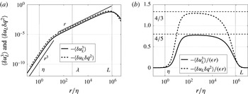
), this is not the case for the helical ‘four-thirds’ law. Both these fundamental relations will be assessed numerically here at high Reynolds numbers, and statistics of helical flows will be further investigated, notably the evolution equation of the helical dissipation rate
 $\unicode[STIX]{x1D716}_{H}$
and derivatives of skew-isotropic tensors.
Finally, a new configuration is addressed, combining both a mean scalar gradient and helicity. This case, which could be of interest for the modelling of atmospheric turbulence where these two features may be present, permits us to illustrate the subtle effects of helicity on the scalar flux, or two-point spectral velocity–scalar correlation. Indeed, unlike a passive scalar field where there is no explicit contributions of helicity in its evolution equations, the coupling of helicity and the mean scalar gradient creates the quadrature spectrum
 $Q(k,t)$
, linked to the imaginary antisymmetric part of the scalar flux.
The paper is structured as follows: in § 2, the various spectral evolutions equations, along with the EDQNM modelling, are presented for homogeneous helical turbulence. Initial conditions are discussed and it will be considered that helicity is initially present at large scales only, so that the kinetic and helical spectra
 $E(k,t)$
and
 $H(k,t)$
develop conjointly. The first theoretical results are presented in § 3: the assumptions behind the
 $k^{-5/3}$
scaling of
 $E$
and
 $H$
in the inertial range are discussed in § 3.1, along with the possibility of inverse and direct cascades. Then, in § 3.2, non-local expansions are used to predict the large-scale dynamics of the kinetic energy and helical spectra. The decay of kinetic energy and helicity is then investigated both numerically and theoretically in § 4. Furthermore, structure functions in HHT are addressed in § 5: existing theoretical results are recalled and assessed numerically. The evolution equation of the helicity dissipation rate
 $\unicode[STIX]{x1D716}_{H}$
is studied and simplified, and some developments on skew-isotropic tensors are provided, which notably leads to the definitions of a helical Taylor scale and helical-derivative skewness. In § 6, the evolution equation of the quadrature spectrum is derived, and its inertial scaling is analysed. Finally, the results are recalled and discussed in the concluding § 7.
2 Evolution equations and EDQNM modelling
In this part, the evolution equations of the kinetic and helical spectra are derived starting from the spectral counterpart of the Navier–Stokes equation. In addition, the EDQNM approach is presented in order to compute explicitly the nonlinear transfers involved in these equations. The final resulting EDQNM evolution equations of the kinetic and helical spectra (2.31) and (2.32) given here were derived in Pouquet, Frisch & Léorat (Reference Pouquet, Frisch and Léorat1976), André & Lesieur (Reference André and Lesieur1977), but the main features of the derivation are nevertheless recalled. For consistency purposes, the same formalism as in Mons, Cambon & Sagaut (Reference Mons, Cambon and Sagaut2016), Briard et al. (Reference Briard, Gomez and Cambon2016) is used, so that the present approach could be easily extended to more complex configurations in future works, such as helical-shear flows for instance. In the following, helicity is injected initially at large scales along with kinetic energy so that both decay freely: there is no forcing mechanism or rotation and no magnetic field. Historically, this is the framework investigated by Brissaud et al. (Reference Brissaud, Frisch, Leorat, Lesieur and Mazure1973) and it will be shown that even in such a classical case, there are still some important open questions which are tackled in §§ 3–5, such as the prediction of the helicity decay and its impact on kinetic energy.
2.1 Craya equation
In this part, the evolution equation of the spectral two-point velocity correlation is obtained in the framework of HHT, without any mean-velocity gradient nor rotation. The evolution equation of the spectral fluctuating velocity
 $\hat{u} _{i}$
reads
 $$\begin{eqnarray}\displaystyle \left(\frac{\unicode[STIX]{x2202}}{\unicode[STIX]{x2202}t}+\unicode[STIX]{x1D708}k^{2}\right)\hat{u} _{i}(\boldsymbol{k},t)+\text{i}k_{j}\widehat{u_{i}u_{j}}(\boldsymbol{k})=-\text{i}k_{i}\hat{p}(\boldsymbol{k}), & & \displaystyle\end{eqnarray}$$
which is the spectral counterpart of the Navier–Stokes equation, with
 $\unicode[STIX]{x1D708}$
the kinematic viscosity,
 $k_{i}$
the wavenumber,
 $\hat{p}$
the spectral fluctuating pressure,
 $\text{i}^{2}=-1$
and
 $\hat{()}$
denotes the Fourier transform. The pressure term is cancelled by projecting this equation onto the plane perpendicular to
 $\hat{u} _{i}$
, by virtue of the incompressibility condition
 $k_{i}\hat{u} _{i}=0$
. From this point, one needs to define the two-point second-order velocity correlation
 $\hat{\unicode[STIX]{x1D619}}_{ij}$
, also called the spectral Reynolds tensor
 $$\begin{eqnarray}\displaystyle \hat{\unicode[STIX]{x1D619}}_{ij}(\boldsymbol{k},t)\unicode[STIX]{x1D6FF}(\boldsymbol{k}-\boldsymbol{p})=\left(\frac{1}{2\unicode[STIX]{x03C0}}\right)^{3}\unicode[STIX]{x1D6FF}(\boldsymbol{k}-\boldsymbol{p})\int \text{e}^{-\text{i}\boldsymbol{k}\cdot \boldsymbol{r}}\unicode[STIX]{x1D619}_{ij}(\boldsymbol{r})\,\text{d}^{3}\boldsymbol{r}=\langle \hat{u} _{i}^{\ast }(\boldsymbol{p},t)\hat{u} _{j}(\boldsymbol{k},t)\rangle , & & \displaystyle\end{eqnarray}$$
where
 $\boldsymbol{k}$
and
 $\boldsymbol{p}$
are wave vectors,
 $()^{\ast }$
is the complex conjugate,
 $\langle \cdot \rangle$
an ensemble average and
 $\unicode[STIX]{x1D619}_{ij}$
is the second-order velocity correlation in physical space
 $$\begin{eqnarray}\displaystyle \unicode[STIX]{x1D619}_{ij}(\boldsymbol{r})=\langle u_{i}(\boldsymbol{x})u_{j}(\boldsymbol{x}+\boldsymbol{r})\rangle , & & \displaystyle\end{eqnarray}$$
where
 $\boldsymbol{r}$
is the separation vector, and with in particular
 $\unicode[STIX]{x1D619}_{ii}(0)=\langle u_{i}u_{i}\rangle =2K$
. The evolution equation of
 $\hat{\unicode[STIX]{x1D619}}_{ij}$
, the so-called Craya equation, is
 $$\begin{eqnarray}\displaystyle \left(\frac{\unicode[STIX]{x2202}}{\unicode[STIX]{x2202}t}+2\unicode[STIX]{x1D708}k^{2}\right)\hat{\unicode[STIX]{x1D619}}_{ij}(\boldsymbol{k},t)=T_{ij}^{NL}(\boldsymbol{k},t), & & \displaystyle\end{eqnarray}$$
where
 $T_{ij}^{NL}$
is the total nonlinear and conservative transfer. This nonlinear transfer can be expressed as a function of
 $S_{ijn}$
, the three-point third-order velocity correlation
 $$\begin{eqnarray}\displaystyle S_{ijn}(\boldsymbol{k},\boldsymbol{p},t)\unicode[STIX]{x1D6FF}(\boldsymbol{k}+\boldsymbol{p}+\boldsymbol{q})=\text{i}\langle \hat{u} _{i}(\boldsymbol{q},t)\hat{u} _{j}(\boldsymbol{k},t)\hat{u} _{n}(\boldsymbol{p},t)\rangle , & & \displaystyle\end{eqnarray}$$
so that (Sagaut & Cambon Reference Sagaut and Cambon2008)
 $$\begin{eqnarray}\displaystyle T_{ij}^{NL}(\boldsymbol{k},t)=P_{imn}(\boldsymbol{k})\int S_{nmj}(\boldsymbol{k},\boldsymbol{p},t)\,\text{d}^{3}\boldsymbol{p}+P_{jmn}(\boldsymbol{k})\int S_{nmi}^{\ast }(\boldsymbol{k},\boldsymbol{p},t)\,\text{d}^{3}\boldsymbol{p}, & & \displaystyle\end{eqnarray}$$
where
 $P_{imn}$
is the Kraichnan operator defined as
 $$\begin{eqnarray}\displaystyle P_{imn}(\boldsymbol{k})={\textstyle \frac{1}{2}}(k_{m}P_{in}(\boldsymbol{k})+k_{n}P_{im}(\boldsymbol{k})),\quad \text{with }P_{ij}(\boldsymbol{k})=\unicode[STIX]{x1D6FF}_{ij}-\unicode[STIX]{x1D6FC}_{i}\unicode[STIX]{x1D6FC}_{j}, & & \displaystyle\end{eqnarray}$$
with
 $\unicode[STIX]{x1D6FC}_{i}=k_{i}/k$
. In the following § 2.2, the spectral Reynolds tensor is expressed as a function of the energy and helical densities
 ${\mathcal{E}}$
and
 ${\mathcal{H}}$
, in a procedure similar to what was done recently in the framework of homogeneous anisotropic turbulence (Mons et al.
Reference Mons, Cambon and Sagaut2016). Then, in § 2.3, the nonlinear transfer
 $T_{ij}^{NL}$
is derived with a classical EDQNM procedure.
2.2
 ${\mathcal{E}}$
–
${\mathcal{H}}$
decomposition


In HHT, the spectral Reynolds tensor is not symmetric and real anymore, since it contains an imaginary antisymmetric part (Cambon & Jacquin Reference Cambon and Jacquin1989) reflecting the breakdown of mirror symmetry. Consequently,
 $\hat{\unicode[STIX]{x1D619}}_{ij}$
can be written
 $$\begin{eqnarray}\displaystyle \hat{\unicode[STIX]{x1D619}}_{ij}(\boldsymbol{k},t)={\mathcal{E}}(\boldsymbol{k},t)P_{ij}+\text{i}\unicode[STIX]{x1D716}_{ijk}\unicode[STIX]{x1D6FC}_{k}\frac{{\mathcal{H}}(\boldsymbol{k},t)}{k}, & & \displaystyle\end{eqnarray}$$
where
 $\unicode[STIX]{x1D716}_{ijk}$
is the Levi-Civita permutation tensor. Similar decompositions were used by Borue & Orszag (Reference Borue and Orszag1997), Chen et al. (Reference Chen, Chen and Eyink2003). From this rather simple decomposition, one could extend to more complex cases containing polarization and directional anisotropies, such as helical-shear driven turbulence, whose equations are given in Cambon et al. (Reference Cambon, Danaila, Godeferd and Scott2013). The energy and helical densities
 ${\mathcal{E}}$
and
 ${\mathcal{H}}$
are linked to the spectral Reynolds tensor
 $\hat{\unicode[STIX]{x1D619}}_{ij}$
through
 $$\begin{eqnarray}\displaystyle {\mathcal{E}}(\boldsymbol{k},t)={\textstyle \frac{1}{2}}\hat{\unicode[STIX]{x1D619}}_{ii}(\boldsymbol{k},t),\quad {\mathcal{H}}(\boldsymbol{k},t)=-{\textstyle \frac{1}{2}}\text{i}k_{m}\unicode[STIX]{x1D716}_{ijm}\hat{\unicode[STIX]{x1D619}}_{ij}(\boldsymbol{k},t). & & \displaystyle\end{eqnarray}$$
The helical density
 ${\mathcal{H}}$
can also be defined in terms of the spectral fluctuating velocity and vorticity
 $$\begin{eqnarray}\displaystyle {\mathcal{H}}(\boldsymbol{k},t)\unicode[STIX]{x1D6FF}(\boldsymbol{k}-\boldsymbol{p})=\left(\frac{1}{2\unicode[STIX]{x03C0}}\right)^{3}\unicode[STIX]{x1D6FF}(\boldsymbol{k}-\boldsymbol{p})\int \text{e}^{-\text{i}\boldsymbol{k}\cdot \boldsymbol{r}}\unicode[STIX]{x1D619}_{ii}^{H}(\boldsymbol{r})\,\text{d}^{3}\boldsymbol{r}=\frac{1}{2}\langle \hat{u} _{i}^{\ast }(\boldsymbol{p},t)\hat{\unicode[STIX]{x1D714}}_{i}(\boldsymbol{k},t)\rangle , & & \displaystyle\end{eqnarray}$$
where
 $\unicode[STIX]{x1D619}_{ij}^{H}$
is the second-order velocity–vorticity correlation in physical space
 $$\begin{eqnarray}\displaystyle \unicode[STIX]{x1D619}_{ij}^{H}(\boldsymbol{r})=\langle u_{i}(\boldsymbol{x})\unicode[STIX]{x1D714}_{j}(\boldsymbol{x}^{\prime })\rangle , & & \displaystyle\end{eqnarray}$$
with in particular
 $\unicode[STIX]{x1D619}_{ii}^{H}(0)=2K_{H}$
. The evolution equations of the kinetic energy and helical densities are then
 $$\begin{eqnarray}\displaystyle \left(\frac{\unicode[STIX]{x2202}}{\unicode[STIX]{x2202}t}+2\unicode[STIX]{x1D708}k^{2}\right){\mathcal{E}}(\boldsymbol{k},t)=T_{{\mathcal{E}}}(\boldsymbol{k},t),\quad \left(\frac{\unicode[STIX]{x2202}}{\unicode[STIX]{x2202}t}+2\unicode[STIX]{x1D708}k^{2}\right){\mathcal{H}}(\boldsymbol{k},t)=T_{{\mathcal{H}}}(\boldsymbol{k},t). & & \displaystyle\end{eqnarray}$$
Afterwards, to express
 $T_{{\mathcal{E}}}$
and
 $T_{{\mathcal{H}}}$
as a function of
 $T_{ij}^{NL}$
, one has to use the tensor
 $$\begin{eqnarray}\displaystyle \unicode[STIX]{x1D70F}_{ij}(\boldsymbol{k},t)=k_{n}\int S_{ijn}(\boldsymbol{k},\boldsymbol{p},t)d^{3}\boldsymbol{p}, & & \displaystyle\end{eqnarray}$$
where
 $S_{ijn}$
is the three-point third-order velocity correlation defined in (2.5). This procedure, used recently in Briard et al. (Reference Briard, Gomez and Cambon2016), Mons et al. (Reference Mons, Cambon and Sagaut2016) in the framework of homogeneous anisotropic turbulence, permits us to express the total nonlinear transfer as
 $$\begin{eqnarray}\displaystyle T_{ij}^{NL}(\boldsymbol{k},t)=P_{in}(\boldsymbol{k})\unicode[STIX]{x1D70F}_{nj}(\boldsymbol{k},t)+P_{jn}(\boldsymbol{k})\unicode[STIX]{x1D70F}_{ni}^{\ast }(\boldsymbol{k},t). & & \displaystyle\end{eqnarray}$$
One obtains
 $$\begin{eqnarray}\displaystyle & \displaystyle T_{{\mathcal{E}}}(\boldsymbol{k},t)={\textstyle \frac{1}{2}}T_{ii}^{NL}(\boldsymbol{k},t)={\textstyle \frac{1}{2}}(\unicode[STIX]{x1D70F}_{ii}(\boldsymbol{k},t)+\unicode[STIX]{x1D70F}_{ii}^{\ast }(\boldsymbol{k},t)), & \displaystyle\end{eqnarray}$$
 $$\begin{eqnarray}\displaystyle & \displaystyle T_{{\mathcal{H}}}(\boldsymbol{k},t)=-{\textstyle \frac{1}{2}}\text{i}\unicode[STIX]{x1D716}_{ijl}k_{l}(\unicode[STIX]{x1D70F}_{ij}(\boldsymbol{k},t)+\unicode[STIX]{x1D70F}_{ji}^{\ast }(\boldsymbol{k},t)), & \displaystyle\end{eqnarray}$$
and the latter expression was notably derived in Cambon & Jacquin (Reference Cambon and Jacquin1989).
The kinetic energy and helical spectra
 $E(k,t)$
and
 $H(k,t)$
are defined as the spherical average of the kinetic energy and helical densities
 $$\begin{eqnarray}\displaystyle E(k,t)=\int _{S_{k}}{\mathcal{E}}(\boldsymbol{k},t)\,\text{d}^{2}\boldsymbol{k},\quad H(k,t)=\int _{S_{k}}{\mathcal{H}}(\boldsymbol{k},t)\,\text{d}^{2}\boldsymbol{k}, & & \displaystyle\end{eqnarray}$$
and in HHT, the spherical integration amounts to a multiplication by
 $4\unicode[STIX]{x03C0}k^{2}$
. The evolution equations of both
 $E$
and
 $H$
are given in § 2.3 along with the spherical average of
 $T_{{\mathcal{E}}}$
and
 $T_{{\mathcal{H}}}$
. The kinetic energy and its dissipation rate are computed as
 $$\begin{eqnarray}\displaystyle K(t)=\frac{\langle u_{i}u_{i}\rangle }{2}=\int _{0}^{\infty }E(k,t)\,\text{d}k,\quad \unicode[STIX]{x1D716}(t)=\unicode[STIX]{x1D708}\left\langle \frac{\unicode[STIX]{x2202}u_{i}}{\unicode[STIX]{x2202}x_{j}}\frac{\unicode[STIX]{x2202}u_{i}}{\unicode[STIX]{x2202}x_{j}}\right\rangle =2\unicode[STIX]{x1D708}\int _{0}^{\infty }k^{2}E(k,t)\,\text{d}k.\qquad \quad & & \displaystyle\end{eqnarray}$$
Similarly, one has for the helicity and its dissipation rate
 $$\begin{eqnarray}\displaystyle K_{H}(t)=\frac{\langle u_{i}\unicode[STIX]{x1D714}_{i}\rangle }{2}=\int _{0}^{\infty }H(k,t)\,\text{d}k,\quad \unicode[STIX]{x1D716}_{H}(t)=\unicode[STIX]{x1D708}\left\langle \frac{\unicode[STIX]{x2202}u_{i}}{\unicode[STIX]{x2202}x_{j}}\frac{\unicode[STIX]{x2202}\unicode[STIX]{x1D714}_{i}}{\unicode[STIX]{x2202}x_{j}}\right\rangle =2\unicode[STIX]{x1D708}\int _{0}^{\infty }k^{2}H(k,t)\,\text{d}k. & & \displaystyle \nonumber\\ \displaystyle & & \displaystyle\end{eqnarray}$$
The kinetic energy and helicity evolution equations in freely decaying turbulence are
 $$\begin{eqnarray}\displaystyle \frac{\text{d}K}{\text{d}t}=-\unicode[STIX]{x1D716},\quad \frac{\text{d}K_{H}}{\text{d}t}=-\unicode[STIX]{x1D716}_{H}, & & \displaystyle\end{eqnarray}$$
and the decay of these quantities for high Reynolds numbers is investigated in § 4. We define as well the kinetic and helical integral scales
 $$\begin{eqnarray}\displaystyle L(t)=\frac{3\unicode[STIX]{x03C0}}{4K}\int _{0}^{\infty }k^{-1}E(k,t)\,\text{d}k,\quad L_{H}(t)=\frac{3\unicode[STIX]{x03C0}}{4K_{H}}\int _{0}^{\infty }k^{-1}H(k,t)\,\text{d}k. & & \displaystyle\end{eqnarray}$$
Finally, from the definition of the vorticity itself, it can be shown that the helical spectrum
 $H(k,t)$
must satisfy the following condition (Kraichnan Reference Kraichnan1973)
 $$\begin{eqnarray}\displaystyle |H(k,t)|\leqslant kE(k,t), & & \displaystyle\end{eqnarray}$$
with
 $K_{H}=\langle u_{i}\unicode[STIX]{x1D714}_{i}\rangle /2$
. At this level, one must point out that unlike kinetic energy which is always positive, helicity is not positive definite and consequently can be negative, so that
 $H(k,t)$
can take negative values.
2.3 EDQNM closure and nonlinear transfers
The EDQNM approximation is now used to close the nonlinear transfers
 $T_{{\mathcal{E}}}$
and
 $T_{{\mathcal{H}}}$
that call into play the triple correlation
 $S_{ijn}$
. The complete procedure is detailed and discussed in numerous references (Pouquet et al.
Reference Pouquet, Frisch and Léorat1976; André & Lesieur Reference André and Lesieur1977; Lesieur Reference Lesieur2008; Sagaut & Cambon Reference Sagaut and Cambon2008) and has been used recently in homogeneous isotropic turbulence (Briard et al.
Reference Briard, Gomez, Sagaut and Memari2015). Consequently, only a brief description is presented here.
The EDQNM model was firstly introduced by Orszag (Reference Orszag1970), Leith (Reference Leith1971), Orszag (Reference Orszag, Balian and Peube1977) for hydrodynamic turbulence. This approximation is used here to solve the equations of dynamics in order to obtain the time evolution of the kinetic and helical spectra. The EDQNM model is a quasi-normal closure: this approximation assumes that the fourth-order moments of the velocity field appearing in the evolution equation of the third-order correlation are related to the second-order moments as if the field was Gaussian. The realizability of the model is then enforced by adding an eddy-damping term
 $$\begin{eqnarray}\displaystyle \unicode[STIX]{x1D702}^{ED}(k,t)=A\sqrt{\int _{0}^{k}p^{2}E(p,t)\,\text{d}p} & & \displaystyle\end{eqnarray}$$
that reflects departure from Gaussianity, where the Kolmogorov constant
 $C_{E}\simeq 1.30$
with
 $A=0.355$
. The Markovianization leads to define the relaxation time of the third-order correlations in the EDQNM model as
 $$\begin{eqnarray}\displaystyle \unicode[STIX]{x1D703}_{kpq}=\frac{1-\text{e}^{-\unicode[STIX]{x1D707}_{kpq}t}}{\unicode[STIX]{x1D707}_{kpq}}\quad \text{where}~\unicode[STIX]{x1D707}_{kpq}=\unicode[STIX]{x1D708}(k^{2}+p^{2}+q^{2})+\unicode[STIX]{x1D702}^{ED}(k,t)+\unicode[STIX]{x1D702}^{ED}(p,t)+\unicode[STIX]{x1D702}^{ED}(q,t). & & \displaystyle \nonumber\\ \displaystyle & & \displaystyle\end{eqnarray}$$
When it comes to the study of helicity, an additional assumption is made, as in André & Lesieur (Reference André and Lesieur1977): the characteristic time of the third-order correlations
 $\unicode[STIX]{x1D703}_{kpq}$
is chosen to be the same for the kinetic and helical fields. It is shown in § 3.1 that such an hypothesis is consistent with joint cascades for the kinetic and helical spectra, and can be a posteriori justified with physical arguments. Beyond these physical justifications, it seems consistent to choose
 $\unicode[STIX]{x1D703}_{kpq}$
for both the kinetic and helical fields since the closure comes from the same evolution equation, which is the one of the third-order correlation defined in (2.5).
Thanks to the EDQNM approximation, one can compute explicitly the spherical average of the nonlinear kinetic and helical transfers, as done in André & Lesieur (Reference André and Lesieur1977), which yields
 $$\begin{eqnarray}\displaystyle & \displaystyle S_{E}^{NL}(k,t)=\int _{S_{k}}T_{{\mathcal{E}}}(\boldsymbol{k},t)\,\text{d}^{2}\boldsymbol{k}=S^{(iso)}(k,t)+S^{(hel)}(k,t), & \displaystyle\end{eqnarray}$$
 $$\begin{eqnarray}\displaystyle & \displaystyle S_{H}^{NL}(k,t)=\int _{S_{k}}T_{{\mathcal{H}}}(\boldsymbol{k},t)\,\text{d}^{2}\boldsymbol{k}=S_{H}^{(dir)}(k,t)+S_{H}^{(inv)}(k,t), & \displaystyle\end{eqnarray}$$
with in detail
 $$\begin{eqnarray}\displaystyle & \displaystyle S^{(iso)}(k,t)=16\unicode[STIX]{x03C0}^{2}\int _{\unicode[STIX]{x1D6E5}_{k}}\unicode[STIX]{x1D703}_{kpq}k^{2}p^{2}q(xy+z^{3}){\mathcal{E}}^{\prime \prime }({\mathcal{E}}^{\prime }-{\mathcal{E}})\,\text{d}p\,\text{d}q, & \displaystyle\end{eqnarray}$$
 $$\begin{eqnarray}\displaystyle & \displaystyle S^{(hel)}(k,t)=-16\unicode[STIX]{x03C0}^{2}\int _{\unicode[STIX]{x1D6E5}_{k}}\unicode[STIX]{x1D703}_{kpq}k^{2}pz(x+yz){\mathcal{H}}^{\prime \prime }({\mathcal{H}}^{\prime }-{\mathcal{H}})\,\text{d}p\,\text{d}q, & \displaystyle\end{eqnarray}$$
 $$\begin{eqnarray}\displaystyle & \displaystyle S_{H}^{(dir)}(k,t)=16\unicode[STIX]{x03C0}^{2}\int _{\unicode[STIX]{x1D6E5}_{k}}\unicode[STIX]{x1D703}_{kpq}k^{2}p^{2}q(xy+z^{3}){\mathcal{E}}^{\prime \prime }({\mathcal{H}}^{\prime }-{\mathcal{H}})\,\text{d}p\,\text{d}q, & \displaystyle\end{eqnarray}$$
 $$\begin{eqnarray}\displaystyle & \displaystyle S_{H}^{(inv)}(k,t)=-16\unicode[STIX]{x03C0}^{2}\int _{\unicode[STIX]{x1D6E5}_{k}}\unicode[STIX]{x1D703}_{kpq}k^{2}pz(x+yz){\mathcal{H}}^{\prime \prime }(p^{2}{\mathcal{E}}^{\prime }-k^{2}{\mathcal{E}})\,\text{d}p\,\text{d}q, & \displaystyle\end{eqnarray}$$
with
 $\unicode[STIX]{x1D6E5}_{k}$
the domain where
 $k$
,
 $p$
and
 $q$
are the lengths of the sides of the triangle formed by the triad
 $\boldsymbol{k}+\boldsymbol{p}+\boldsymbol{q}=\mathbf{0}$
, and where
 $x$
,
 $y$
and
 $z$
are the cosines of the angles formed by
 $\boldsymbol{p}$
and
 $\boldsymbol{q}$
,
 $\boldsymbol{q}$
and
 $\boldsymbol{k}$
, and
 $\boldsymbol{k}$
and
 $\boldsymbol{p}$
respectively. For the sake of clarity
 ${\mathcal{E}}=E(k,t)/4\unicode[STIX]{x03C0}k^{2}$
,
 ${\mathcal{E}}^{\prime }=E(p,t)/4\unicode[STIX]{x03C0}p^{2}$
and
 ${\mathcal{E}}^{\prime \prime }=E(q,t)/4\unicode[STIX]{x03C0}q^{2}$
, and
 ${\mathcal{H}}=H(k,t)/4\unicode[STIX]{x03C0}k^{2}$
,
 ${\mathcal{H}}^{\prime }=H(p,t)/4\unicode[STIX]{x03C0}p^{2}$
and
 ${\mathcal{H}}^{\prime \prime }=H(q,t)/4\unicode[STIX]{x03C0}q^{2}$
. These four nonlinear transfers
 $S^{(iso)}$
,
 $S^{(hel)}$
,
 $S_{H}^{(dir)}$
, and
 $S_{H}^{(inv)}$
are conservative (with zero integral over the whole wavenumber space) and have been obtained previously (André & Lesieur Reference André and Lesieur1977). Here is some additional information:
 $S^{(iso)}$
is the classical kinetic energy nonlinear transfer appearing in HIT. Moreover, it is clear from (2.25) that helicity directly impacts the nonlinear transfers of
 $E(k,t)$
through a purely helical transfer
 $S^{(hel)}$
. One can further remark that
 $S_{H}^{(dir)}$
has a form very similar to the isotropic nonlinear transfer of a passive scalar field (Briard et al.
Reference Briard, Gomez and Cambon2016). In addition to the original work of André & Lesieur (Reference André and Lesieur1977), it will be shown numerically in § 3.1 that both
 $S^{(iso)}$
and
 $S_{H}^{(dir)}$
correspond to direct transfers from large to small scales, whereas
 $S^{(hel)}$
and
 $S_{H}^{(inv)}$
are inverse transfers.
Finally, with (2.25) and (2.26), it is now possible to write the Lin evolution equations for
 $E(k,t)$
and
 $H(k,t)$
in homogeneous helical turbulence
 $$\begin{eqnarray}\displaystyle & \displaystyle \left(\frac{\unicode[STIX]{x2202}}{\unicode[STIX]{x2202}t}+2\unicode[STIX]{x1D708}k^{2}\right)E(k,t) & \displaystyle =S_{E}^{NL}(k,t),\end{eqnarray}$$
 $$\begin{eqnarray}\displaystyle & \displaystyle \left(\frac{\unicode[STIX]{x2202}}{\unicode[STIX]{x2202}t}+2\unicode[STIX]{x1D708}k^{2}\right)H(k,t) & \displaystyle =S_{H}^{NL}(k,t).\end{eqnarray}$$
In the next part, some details are provided about the numerical resolution of these two equations.
2.4 Numerical set-up and initial conditions
The time evolution of the kinetic and helical spectra
 $E(k,t)$
and
 $H(k,t)$
is obtained by solving two coupled integro-differential equations using a third-order Runge–Kutta scheme with implicit treatment of viscous terms. The wavenumber space is discretized using a logarithmic mesh
 $k_{i+1}=rk_{i}$
for
 $i=1,\ldots ,n$
, where
 $n$
is the total number of modes and
 $r=10^{1/f}$
,
 $f=17$
being the number of points per decade. This mesh spans from
 $k_{min}=10^{-6}k_{L}$
to
 $k_{max}=10k_{\unicode[STIX]{x1D702}}$
, where
 $k_{L}=1/L$
is the integral wavenumber and
 $k_{\unicode[STIX]{x1D702}}=(\unicode[STIX]{x1D716}/\unicode[STIX]{x1D708}^{3})^{1/4}$
is the Kolmogorov wavenumber (the possibility of a different viscous cutoff wavenumber for the helical spectrum will be discussed as well). If not mentioned otherwise, the initial Reynolds number based on the Taylor microscale is
 $Re_{\unicode[STIX]{x1D706}}(0)\simeq 5\times 10^{4}$
: this allows us to investigate the decay of helicity and kinetic energy in regimes that cannot be reached yet by DNS, but that nevertheless involve typical Reynolds numbers of atmospheric flows. The characteristic time used for normalization is the eddy turnover time
 $\unicode[STIX]{x1D70F}_{0}=K(0)/\unicode[STIX]{x1D716}(0)$
.
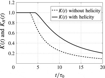
Early decay of the kinetic energy
 $K(t)$
with and without the additional presence of helicity, for Batchelor turbulence (
 $\unicode[STIX]{x1D70E}=4$
). The results are similar for Saffman turbulence (
 $\unicode[STIX]{x1D70E}=2$
).

The choice of initial conditions is important, and for consistency, the same as in André & Lesieur (Reference André and Lesieur1977) are used
 $$\begin{eqnarray}\displaystyle E(k,t=0)=k^{\unicode[STIX]{x1D70E}}\exp \left(-\frac{\unicode[STIX]{x1D70E}}{2}\left(\frac{k}{k_{L}}\right)^{2}\right),\quad H(k,t=0)=kE(k,t=0), & & \displaystyle\end{eqnarray}$$
with
 $\unicode[STIX]{x1D70E}$
the large-scale spectral exponent of the kinetic energy spectrum:
 $E(k<k_{L})\sim k^{\unicode[STIX]{x1D70E}}$
. Consequently, the helical infrared slope is
 $\unicode[STIX]{x1D70E}_{H}=\unicode[STIX]{x1D70E}+1$
and satisfies (2.22). It can be checked numerically that if one chooses
 $E(k,0)=H(k,0)$
, this violates the previous condition at large scales. Moreover, with the choice (2.33), both spectra evolve conjointly, and helicity affects the filling of the small scales during the cascade of kinetic energy: this is illustrated in figure 1 as well, where the filling of the small scales with kinetic energy is delayed by helicity at the early times of the decay. This is consistent with the results of André & Lesieur (Reference André and Lesieur1977). The authors insist on the fact that the first effect of helicity is to slightly slow down the filling of small scales with energy, as already noticed by Polifke & Shtilman (Reference Polifke and Shtilman1989), Polifke (Reference Polifke1991), Moffatt & Tsinober (Reference Moffatt and Tsinober1992). Once the spectra
 $E$
and
 $H$
are fully developed, the effects of helicity on the kinetic energy decay are more subtle, as addressed in §§ 3.2 and 4.
3 Kinetic energy and helical spectra
$E(k,t)$
and
$H(k,t)$


In this part, the kinetic energy and helical spectra
 $E(k,t)$
and
 $H(k,t)$
are investigated numerically at very large Reynolds numbers thanks to the EDQNM modelling presented in the previous section. Firstly, basic properties of homogeneous skew-isotropic flows are recovered and some features regarding inverse transfers are addressed. Then, non-local interactions are considered in the infrared range of the spectra (for wavenumbers smaller than the integral one
 $k_{L}$
) and non-local expansions are made in order to study the large-scale dynamics. These results will be directly used in § 4 to predict the decay of kinetic energy and helicity in homogeneous turbulence.
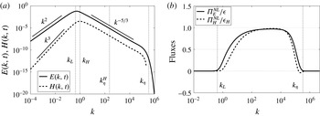
(a) Kinetic and helical spectra
 $E(k,t)$
and
 $H(k,t)$
.
 $k_{\unicode[STIX]{x1D702}}^{H}$
is defined in (3.1), and
 $k_{H}$
is the helical integral wavenumber. (b) Normalized kinetic and helical fluxes with their respective dissipation rates
 $\unicode[STIX]{x1D716}$
and
 $\unicode[STIX]{x1D716}_{H}$
. Both with
 $\unicode[STIX]{x1D70E}=2$
, at
 $Re_{\unicode[STIX]{x1D706}}=2\times 10^{4}$
, along with the kinetic integral and Kolmogorov wavenumbers
 $k_{L}$
and
 $k_{\unicode[STIX]{x1D702}}$
.

3.1 Joint cascades – direct and inverse nonlinear transfers
Since the numerical work of Chen et al. (Reference Chen, Chen and Eyink2003), the joint cascades of the kinetic energy and helicity in
 $k^{-5/3}$
inertial ranges have been well assessed. This section aims at exploring large Reynolds numbers with EDQNM, as done in the pioneering study of André & Lesieur (Reference André and Lesieur1977): more precisely, higher Reynolds numbers are reached, the assumptions and physics behind the
 $k^{-5/3}$
scaling of the kinetic energy and helical spectra are discussed and the spectral nonlinear transfers of kinetic energy and helicity are investigated in order to exhibit some inverse transfer mechanisms.
Firstly, the
 $k^{-5/3}$
scaling for both
 $E$
and
 $H$
is presented in figure 2. The inertial kinetic and helical ranges both extend from their respective integral wavenumbers
 $k_{L}=1/L$
and
 $k_{H}=1/L_{H}$
to the Kolmogorov wavenumber
 $k_{\unicode[STIX]{x1D702}}$
. It was argued in Ditlevsen & Giuliani (Reference Ditlevsen and Giuliani2001) that there could be a different cutoff for the helical spectrum, defined as
 $$\begin{eqnarray}\displaystyle k_{\unicode[STIX]{x1D702}}^{H}=\left(\frac{\unicode[STIX]{x1D716}_{H}^{3}}{\unicode[STIX]{x1D708}^{3}\unicode[STIX]{x1D716}^{2}}\right)^{1/7}. & & \displaystyle\end{eqnarray}$$
The opposite was proposed by Chen et al. (Reference Chen, Chen and Eyink2003), i.e. there is only one viscous cutoff
 $k_{\unicode[STIX]{x1D702}}$
. The latter is clearly what is obtained in figure 2: the
 $k^{-5/3}$
ranges for
 $E$
and
 $H$
both reach
 $k_{\unicode[STIX]{x1D702}}$
. It is worth noting that at moderate Reynolds numbers
 $Re_{\unicode[STIX]{x1D706}}\sim 50$
,
 $k_{\unicode[STIX]{x1D702}}$
is only three to four times higher than
 $k_{\unicode[STIX]{x1D702}}^{H}$
: consequently, large Reynolds numbers are needed to assess that the helical inertial range reaches the Kolmogorov wavenumber. Another interpretation of
 $k_{\unicode[STIX]{x1D702}}^{H}$
is proposed in appendix E. Helicity being a quantity not positive definite, a change of sign can be observed in
 $H(k,t)$
: more precisely here, negative values are obtained at small scales. Such a phenomenon also occurred at large Reynolds numbers in André & Lesieur (Reference André and Lesieur1977), and was observed as well at moderate Reynolds numbers in DNS (Polifke & Shtilman Reference Polifke and Shtilman1989; Polifke Reference Polifke1991).
The
 $k^{-5/3}$
scaling can be deduced from dimensional analysis. The main hypothesis is that the typical characteristic time in the inertial range
 $\unicode[STIX]{x1D70F}(k)=(k^{2}\unicode[STIX]{x1D716})^{-1/3}$
is the same for both the kinetic and helical spectra. From this assumption results an ‘Obukhov-like’ scaling,
 $\unicode[STIX]{x1D716}_{H}(t)=kH(k,t)/\unicode[STIX]{x1D70F}(k)$
, which directly yields in the inertial range
 $$\begin{eqnarray}\displaystyle H(k,t)=C_{H}\unicode[STIX]{x1D716}_{H}\unicode[STIX]{x1D716}^{-1/3}k^{-5/3}. & & \displaystyle\end{eqnarray}$$
The constant
 $C_{H}\simeq 2$
is obtained at
 $Re_{\unicode[STIX]{x1D706}}=2\times 10^{4}$
, whereas the Kolmogorov constant remains unchanged with respect to HIT simulations. The present value
 $C_{H}\simeq 2$
is in agreement with André & Lesieur (Reference André and Lesieur1977). It is worth noting that one could change
 $C_{E}$
and
 $C_{H}$
to fit better with DNS by modifying the eddy-damping constants: this is out of the scope of the present work, but could be of interest for the development of simplified models.
One can remark that the scaling (3.2) is very similar to the one of a scalar field being passively advected by a turbulent flow: indeed, a similar assumption regarding the nonlinear time and the scalar dissipation rate is made in this case (see Lesieur (Reference Lesieur2008) for a review). This is one of the reasons why it is often said that helicity cascades linearly with the kinetic energy (André & Lesieur Reference André and Lesieur1977; Ditlevsen & Giuliani Reference Ditlevsen and Giuliani2001).
The scaling (3.2) can also be obtained by considering that nonlinear transfers in the inertial range are mainly local, i.e.
 $k\sim p\sim q$
in (2.27)–(2.30). By dimensional analysis, and dropping all geometric factors
 $x$
,
 $y$
and
 $z$
, this yields for the kinetic and helical fluxes
 $\unicode[STIX]{x1D6F1}(k)\sim \unicode[STIX]{x1D703}E(k)^{2}k^{4}$
and
 $\unicode[STIX]{x1D6F1}_{H}(k)\sim \unicode[STIX]{x1D703}E(k)H(k)k^{4}$
, where the flux is
 $\unicode[STIX]{x1D6F1}\sim kS_{E}^{NL}$
, and
 $\unicode[STIX]{x1D703}=\unicode[STIX]{x1D703}_{kkk}$
is the ‘local’ third-order correlation characteristic time. Using the hypothesis for the eddy damping of the helicity field, which is that
 $\unicode[STIX]{x1D703}_{kpq}$
is identical for both
 $E$
and
 $H$
, and assuming that at high Reynolds numbers in the inertial range one has
 $\unicode[STIX]{x1D6F1}\simeq \unicode[STIX]{x1D716}$
and
 $\unicode[STIX]{x1D6F1}_{H}\simeq \unicode[STIX]{x1D716}_{H}$
, yields
 $$\begin{eqnarray}\displaystyle \unicode[STIX]{x1D703}\sim \frac{\unicode[STIX]{x1D716}}{k^{4}E^{2}}=\unicode[STIX]{x1D70F}(k)=(k^{2}\unicode[STIX]{x1D716})^{-1/3}. & & \displaystyle\end{eqnarray}$$
The latter assumption
 $\unicode[STIX]{x1D6F1}\simeq \unicode[STIX]{x1D716}$
is often made at large Reynolds numbers and is well assessed in figure 2. Finally, using (3.3), one obtains two equivalent relations
 $$\begin{eqnarray}\displaystyle \unicode[STIX]{x1D716}(t)H(k,t)\sim \unicode[STIX]{x1D716}_{H}(t)E(k,t)\quad \text{and}\quad \unicode[STIX]{x1D716}(t)K_{H}(t)\sim \unicode[STIX]{x1D716}_{H}(t)K(t). & & \displaystyle\end{eqnarray}$$
The scaling (3.2) is further recovered by replacing the kinetic energy spectrum by
 $E(k)\sim \unicode[STIX]{x1D716}^{2/3}k^{-5/3}$
. Thus, the joint cascade of kinetic energy and helicity is recovered, and simple arguments showed that the assumption behind the
 $k^{-5/3}$
scaling of
 $H(k,t)$
is that the velocity and helical fields have the same characteristic inertial time
 $\unicode[STIX]{x1D70F}(k)=(k^{2}\unicode[STIX]{x1D716})^{-1/3}$
.
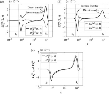
(a) Helical nonlinear transfers
 $S_{H}^{(dir)}$
and
 $S_{H}^{(inv)}$
. (b) Purely helical and isotropic nonlinear transfers
 $S^{(hel)}$
and
 $S^{(iso)}$
. (c) Total nonlinear kinetic and helical transfers
 $kS_{E}^{NL}$
and
 $kS_{H}^{NL}$
. All for Batchelor turbulence (
 $\unicode[STIX]{x1D70E}=4$
) at
 $Re_{\unicode[STIX]{x1D706}}=5\times 10^{3}$
, along with the integral and Kolmogorov wavenumbers
 $k_{L}$
and
 $k_{\unicode[STIX]{x1D702}}$
.

The total nonlinear kinetic and helical transfers
 $S_{E}^{NL}$
and
 $S_{H}^{NL}$
, defined in (2.25) and (2.26) respectively, are now investigated in figure 3 for Batchelor turbulence (results are similar for Saffman turbulence). In § 2.3,
 $S_{E}^{NL}$
was decomposed into the sum of a purely kinetic contribution
 $S^{(iso)}$
, identical to the nonlinear transfer in HIT, and a purely helical contribution
 $S^{(hel)}$
. It is found in the EDQNM simulations that the latter part corresponds in fact to a transfer of energy from small to large scales. This inverse transfer is nevertheless less intense than the direct one, so that the total kinetic transfer
 $S_{E}^{NL}$
is direct. Moreover, whereas the direct nonlinear transfer
 $S^{(iso)}$
spans all scales of the wavenumber space, the inverse transfer
 $S^{(hel)}$
is very localized at large scales, which creates a small region where
 $S^{(iso)}$
is positive at large scales, which is different from HIT. Nevertheless, the total kinetic energy transfer
 $S_{E}^{NL}$
is completely similar to the one in HIT.
Similarly,
 $S_{H}^{NL}$
was decomposed into two contributions
 $S_{H}^{(dir)}$
and
 $S_{H}^{(inv)}$
, which both span the entire inertial range. It is revealed in figure 3 that these two parts correspond to direct and inverse transfers respectively. Once again, the inverse transfer is weaker than the direct one, so that the total transfer of helicity
 $S_{H}^{NL}$
goes from large to small scales. One can observe that
 $S_{H}^{NL}$
is negative around
 $k_{\unicode[STIX]{x1D702}}$
, and this explains the negative values of the helical spectrum
 $H(k,t)$
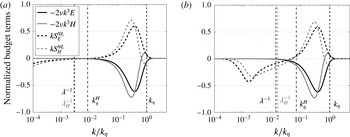
at the dissipative scales observed in figure 2: this can be interpreted as viscous production of helicity, since
 $-2\unicode[STIX]{x1D708}k^{3}H(k)$
is positive in this region. The fact that inverse transfers of kinetic energy and helicity are hidden in the total direct cascade is in agreement with the recent results of Alexakis (Reference Alexakis2017).
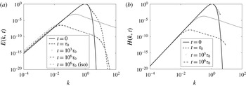
Decaying spectra in Batchelor turbulence (
 $\unicode[STIX]{x1D70E}=4$
) with
 $Re_{\unicode[STIX]{x1D706}}(0)=3400$
. (a) Kinetic energy spectrum
 $E(k,t)$
: at
 $t=10^{6}\unicode[STIX]{x1D70F}_{0}$
,
 $E$
for HIT is displayed as well in grey. (b) Helical spectrum
 $H(k,t)$
.

In this part, it was recovered that in freely decaying HHT, there is a joint cascade of kinetic energy and helicity towards small scales. The main assumption behind the
 $k^{-5/3}$
inertial scaling is that the kinetic and helical fields have the same inertial characteristic time. Finally, it was shown numerically that despite a direct cascade, some inverse nonlinear transfers occur, which are less intense than direct ones.
3.2 Non-local interactions – infrared range dynamics
This section focuses on the permanence of large eddies (PLE) in the presence of helicity, and on non-local interactions between small and large scales. Consequently, at this point, one needs to recall the definition of the PLE hypothesis. Both Saffman and Batchelor turbulence are investigated in this work, whose infrared exponents are respectively
 $\unicode[STIX]{x1D70E}=2$
and
 $\unicode[STIX]{x1D70E}=4$
, where
 $E(k<k_{L},t)=Bk^{\unicode[STIX]{x1D70E}}$
and
 $H(k<k_{H},t)=B_{H}k^{\unicode[STIX]{x1D70E}_{H}}$
. Due to the initial conditions (2.33) where
 $\unicode[STIX]{x1D70E}_{H}=\unicode[STIX]{x1D70E}+1$
, one has for instance in Batchelor turbulence,
 $E(k<k_{L},0)\sim k^{4}$
and
 $H(k<k_{H},0)\sim k^{5}$
.
The PLE hypothesis is said to be true in decaying turbulence for
 $E(k,t)$
(for
 $H(k,t)$
) when both
 $B$
and
 $\unicode[STIX]{x1D70E}$
(
 $B_{H}$
and
 $\unicode[STIX]{x1D70E}_{H}$
) remain constant throughout the decay. If a kinetic energy spectrum with
 $\unicode[STIX]{x1D70E}\leqslant 4$
is imposed initially, then
 $\unicode[STIX]{x1D70E}$
remains constant (Lesieur & Ossia Reference Lesieur and Ossia2000). Regarding
 $B$
, this prefactor is time dependent for values
 $\unicode[STIX]{x1D70E}$
 $\in [\unicode[STIX]{x1D70E}_{c},4]$
where the critical value is located in the range
 $3\leqslant \unicode[STIX]{x1D70E}_{c}\leqslant 4$
(Eyink & Thomson Reference Eyink and Thomson2000; Lesieur & Ossia Reference Lesieur and Ossia2000). Consequently, for Saffman turbulence (
 $\unicode[STIX]{x1D70E}=2$
), the PLE hypothesis is verified, whereas it is not for Batchelor turbulence (
 $\unicode[STIX]{x1D70E}=4$
): this has been assessed numerically in HIT for
 $E(k,t)$
(Meldi & Sagaut Reference Meldi and Sagaut2013) and for a passive scalar
 $E_{T}(k,t)$
(Briard et al.
Reference Briard, Gomez, Sagaut and Memari2015).
In what follows, it is proposed to investigate both numerically and theoretically what are the effects of helicity on the strong backscatter of energy that classically occurs in Batchelor HIT, and to address the permanence of large eddies at the level of the helical spectrum. The starting point is figure 4, where the time evolutions of the kinetic energy and helical spectra
 $E(k,t)$
and
 $H(k,t)$
are displayed for Batchelor turbulence. Two features need to be underlined: firstly, it appears that
 $H$
experiences no backscatter, so that the PLE hypothesis is verified in Batchelor HHT for the helical spectrum, unlike
 $E$
. Secondly, the backscatter for
 $E$
is weaker in the presence of helicity than in HIT, as revealed by the grey curve corresponding to a HIT simulation for
 $E$
, at the same time. These two features can be explained analytically, using non-local expansions. These important results, and especially the fact that the PLE hypothesis is verified for
 $H$
even in Batchelor turbulence, are applied in the next section to determine theoretical decay exponents for
 $K(t)$
and
 $K_{H}(t)$
.
One can show that the non-local kinetic energy transfer acting in the infrared range, i.e. coming from small scales, is
 $$\begin{eqnarray}\displaystyle T^{(iso)-}(k,t)=\frac{14}{15}k^{4}\int _{k_{L}}^{\infty }\unicode[STIX]{x1D703}_{0pp}\frac{E(p)^{2}}{p^{2}}\,\text{d}p-\frac{2}{15}k^{2}E(k)\int _{k_{L}}^{\infty }\unicode[STIX]{x1D703}_{0pp}\left(5E(p)+p\frac{\unicode[STIX]{x2202}E}{\unicode[STIX]{x2202}p}\right)\,\text{d}p. & & \displaystyle \nonumber\\ \displaystyle & & \displaystyle\end{eqnarray}$$
Such expressions were derived in Lesieur & Schertzer (Reference Lesieur and Schertzer1978), Lesieur (Reference Lesieur2008). The first term on the right-hand side is responsible for the backscatter of energy that breaks the PLE hypothesis. The second term on the right-hand side is classically written under the eddy-viscous form
 $-2\unicode[STIX]{x1D708}_{t}k^{2}E$
, and represents a pseudo kinetic energy dissipation, in other words the damping of large scales by small-scale turbulence. To understand why back transfers of energy on
 $E(k,t)$
are decreased with helicity, one has to expand
 $S^{(hel)}$
when
 $k\ll p\sim q$
, which gives
 $$\begin{eqnarray}\displaystyle T^{(hel)-}(k,t)=-\frac{14}{15}k^{4}\int _{k_{L}}^{\infty }\unicode[STIX]{x1D703}_{0pp}\frac{H(p)^{2}}{p^{4}}\,\text{d}p+\frac{2}{15}k^{2}H(k)\int _{k_{L}}^{\infty }\frac{\unicode[STIX]{x1D703}_{0pp}}{p^{2}}\left(9H(p)-p\frac{\unicode[STIX]{x2202}H}{\unicode[STIX]{x2202}p}\right)\,\text{d}p. & & \displaystyle \nonumber\\ \displaystyle & & \displaystyle\end{eqnarray}$$
The first term on the right-hand side modifies the backscatter of energy whereas the second one can also be interpreted as a pseudo-helical dissipation term in
 $-2\unicode[STIX]{x1D708}_{t}^{H}k^{2}H$
. Combining this expression with (3.5) reveals the impact of helicity on the total inverse non-local kinetic transfer in HHT
 $$\begin{eqnarray}\displaystyle T_{E}^{-}(k,t)=\underbrace{\frac{14}{15}k^{4}\int _{k_{L}}^{\infty }\unicode[STIX]{x1D703}_{0pp}\frac{E(p)^{2}}{p^{2}}\left(1-\left(\frac{H(p)}{pE(p)}\right)^{2}\right)\,\text{d}p}_{k^{4}\;backscatter}\underbrace{-2\unicode[STIX]{x1D708}_{t}k^{2}E(k)-2\unicode[STIX]{x1D708}_{t}^{H}k^{2}H(k)}_{damping\;of\;large\;scales}.\quad & & \displaystyle\end{eqnarray}$$
The second term indicates a change in the effects of viscous damping at large scales, which are difficult to quantify. However, for the first term on the right-hand side, one has, using the realizability condition (2.22), i.e.
 $0\leqslant |H|/kE\leqslant 1$
,
 $$\begin{eqnarray}\displaystyle \frac{14}{15}k^{4}\int _{k_{L}}^{\infty }\unicode[STIX]{x1D703}_{0pp}\frac{E(p)^{2}}{p^{2}}\underbrace{\left(1-\left(\frac{H(p)}{pE(p)}\right)^{2}\right)}_{{\leqslant}1}\,\text{d}p\leqslant \underbrace{\frac{14}{15}k^{4}\int _{k_{L}}^{\infty }\unicode[STIX]{x1D703}_{0pp}\frac{E(p)^{2}}{p^{2}}\,\text{d}p}_{Non\text{-}local\;transfer\;in\;HIT}. & & \displaystyle\end{eqnarray}$$
Consequently, the
 $k^{4}$
backscatter of energy of
 $E(k,t)$
is decreased by helicity, with respect to HIT.
Then, similar non-local expansions for
 $S_{H}^{NL}$
yield
 $$\begin{eqnarray}\displaystyle T_{H}^{-}(k,t)=-\frac{2}{15}k^{2}H(k)\int _{k_{L}}^{\infty }\unicode[STIX]{x1D703}_{0pp}\left(5E(p)+p\frac{\unicode[STIX]{x2202}E}{\unicode[STIX]{x2202}p}\right)\,\text{d}p+\frac{14}{15}k^{4}E(k)\int _{k_{L}}^{\infty }\unicode[STIX]{x1D703}_{0pp}\frac{H(p)}{p^{2}}\,\text{d}p. & & \displaystyle \nonumber\\ \displaystyle & & \displaystyle\end{eqnarray}$$
This inverse non-local helical transfer indicates that there is no strong
 $k^{4}$
backscatter that breaks the PLE hypothesis. The first term can be written
 $-2\unicode[STIX]{x1D708}_{t}k^{2}H$
(and was found also in Baerenzung et al.
Reference Baerenzung, Politano, Ponty and Pouquet2008), and the second one is quite original since it involves a pseudo-enstrophy dissipation and could consequently be written
 $-2\unicode[STIX]{x1D708}_{t}^{\unicode[STIX]{x1D714}}k^{4}E$
.
The method used now to describe analytically the infrared dynamics of the kinetic energy and helical spectra in HHT – at first order – is inspired from Lesieur (Reference Lesieur2008), where a similar reasoning is performed for HIT. When the turbulence is fully developed, both spectra scale with
 $E(k,t)\sim B(t)k^{\unicode[STIX]{x1D70E}}$
and
 $H(k,t)\sim B_{H}(t)k^{\unicode[STIX]{x1D70E}_{H}}$
at large scales. In this infrared range, viscous dissipation is negligible, and inverse non-local transfers
 $T_{E}^{-}$
and
 $T_{H}^{-}$
dominate with respect to local ones
 $S_{E}^{NL}$
and
 $S_{H}^{NL}$
. Thus, the simplified Lin equations in the infrared range are
 $\unicode[STIX]{x2202}_{t}E=T_{E}^{-}$
and
 $\unicode[STIX]{x2202}_{t}H=T_{H}^{-}$
, which yields
 $$\begin{eqnarray}\displaystyle & \displaystyle \frac{\text{d}B}{\text{d}t}=\frac{14}{15}k^{4-\unicode[STIX]{x1D70E}}\int _{k_{L}}^{\infty }(\cdots \,)\,\text{d}p-2\unicode[STIX]{x1D708}_{t}k^{2}B(t)-2\unicode[STIX]{x1D708}_{t}^{H}k^{2+\unicode[STIX]{x1D70E}_{H}-\unicode[STIX]{x1D70E}}B_{H}(t), & \displaystyle\end{eqnarray}$$
 $$\begin{eqnarray}\displaystyle & \displaystyle \frac{\text{d}B_{H}}{\text{d}t}=-\frac{2}{15}k^{2}B_{H}(t)\int _{k_{L}}^{\infty }(\cdots \,)\,\text{d}p+\frac{14}{15}k^{4+\unicode[STIX]{x1D70E}-\unicode[STIX]{x1D70E}_{H}}B(t)\int _{k_{L}}^{\infty }(\cdots \,)\,\text{d}p. & \displaystyle\end{eqnarray}$$
With the present initial conditions (2.33), one has
 $\unicode[STIX]{x1D70E}_{H}=\unicode[STIX]{x1D70E}+1$
, but one could think of different initial conditions that would result in a more complex infrared dynamics for
 $E$
and
 $B$
: this is the object of § 4.4. For now, one has
 $\unicode[STIX]{x1D70E}_{H}=\unicode[STIX]{x1D70E}+1$
, and in this case, whatever the infrared slope
 $\unicode[STIX]{x1D70E}$
is, the dissipation terms involving the turbulent eddy viscosities
 $\unicode[STIX]{x1D708}_{t}$
,
 $\unicode[STIX]{x1D708}_{t}^{\unicode[STIX]{x1D714}}$
and
 $\unicode[STIX]{x1D708}_{t}^{H}$
are negligible because
 $k\ll 1$
, so that
 $$\begin{eqnarray}\displaystyle \forall \unicode[STIX]{x1D70E},\quad \frac{\text{d}B_{H}}{\text{d}t}=-2\unicode[STIX]{x1D708}_{t}^{\unicode[STIX]{x1D714}}k^{3}B(t)-2\unicode[STIX]{x1D708}_{t}k^{2}B_{H}(t)\simeq 0. & & \displaystyle\end{eqnarray}$$
 $\text{d}B_{H}/\text{d}t$
is not rigorously zero, since the non-local expansion is kept at the lowest order in
 $k/p\ll 1$
(see appendix A for details) in the infrared range, as done in Lesieur & Schertzer (Reference Lesieur and Schertzer1978), but is equal to some subdominant terms for the dynamics of
 $B_{H}$
, as assessed by figure 4. This means that whatever the large-scale initial conditions
 $\unicode[STIX]{x1D70E}$
are, the PLE hypothesis holds for the helical spectrum
 $H(k,t)$
when
 $\unicode[STIX]{x1D70E}_{H}=\unicode[STIX]{x1D70E}+1$
.
Regarding
 $E(k,t)$
: with the same reasoning, for
 $\unicode[STIX]{x1D70E}\leqslant 3$
, the terms on the right-hand side of (3.10) are negligible, meaning that the PLE hypothesis holds for
 $E(k,t)$
. Whereas for
 $\unicode[STIX]{x1D70E}=4$
,
 $B(t)$
truly depends on time since the first term on the right-hand side is stronger than the two others
 $-2\unicode[STIX]{x1D708}_{t}k^{2}B$
and
 $-2\unicode[STIX]{x1D708}_{t}^{H}k^{3}B_{H}$
, so that
 $$\begin{eqnarray}\displaystyle \forall \unicode[STIX]{x1D70E}\leqslant 3,\quad \frac{\text{d}B}{\text{d}t}\simeq 0, & & \displaystyle\end{eqnarray}$$
 $$\begin{eqnarray}\displaystyle \unicode[STIX]{x1D70E}=4,\quad \frac{\text{d}B}{\text{d}t}\simeq \frac{14}{15}\int _{k_{L}}^{\infty }\unicode[STIX]{x1D703}_{0pp}\frac{E(p)^{2}}{p^{2}}\left(1-\left(\frac{H(p)}{pE(p)}\right)^{2}\right)\,\text{d}p. & & \displaystyle\end{eqnarray}$$
The latter result contains the fact that helicity decreases the backscatter of
 $E(k,t)$
in Batchelor HHT. The different turbulent spectral viscosities introduced previously are summarized in table 1. Details about the non-local expansions are provided in appendix A.
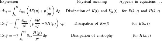
Summary of the different eddy viscosities
 $\unicode[STIX]{x1D708}_{t}$
,
 $\unicode[STIX]{x1D708}_{t}^{H}$
and
 $\unicode[STIX]{x1D708}_{t}^{\unicode[STIX]{x1D714}}$
, that intervene in the non-local expansions of the nonlinear transfers
 $S_{E}^{NL}$
and
 $S_{H}^{NL}$
in HHT.

In conclusion, it has been shown numerically and analytically in this part that firstly the helical spectrum
 $H(k,t)$
does not experience any strong backscatter that breaks the PLE hypothesis, for initial conditions such that
 $\unicode[STIX]{x1D70E}_{H}=\unicode[STIX]{x1D70E}+1$
: in particular, the PLE holds in Batchelor turbulence for
 $H(k,t)$
. And secondly that helicity reduces the backscatter of kinetic energy for
 $E(k,t)$
. These theoretical results regarding the infrared dynamics of
 $H(k,t)$
and the impact of helicity on the infrared dynamics of
 $E(k,t)$
are both directly applied in the following section which aims at predicting the decay of the kinetic energy and helicity at large Reynolds numbers: indeed, the derivation of theoretical decay exponents require an accurate knowledge of the infrared dynamics.
4 Decay exponents for helicity and kinetic energy
The aim of this part is twofold: first, to predict the decay of helicity
 $K_{H}=\langle u_{i}\unicode[STIX]{x1D714}_{i}\rangle /2$
in a homogeneous skew-isotropic turbulent flow when the helical spectrum is initially non-zero, according to (2.33). And secondly to quantify the impact of helicity on the decay of the kinetic energy
 $K(t)=\langle u_{i}u_{i}\rangle /2$
.
4.1 About the interest of the helicity decay
The prediction of the decay of helicity is made possible by the determination, at large Reynolds numbers, of theoretical decay exponents: the method, originally applied in Comte-Bellot & Corrsin (Reference Comte-Bellot and Corrsin1966) (hereafter CBC) for kinetic energy, relies essentially on dimensional analysis. Similar theoretical results regarding the decay of the kinetic energy have also been obtained with self-preservation analysis (George Reference George1992).
Recently, EDQNM has been intensively used to determine these theoretical decay exponents in different configurations, at high Reynolds numbers and after a large number of turnover times: the decay of kinetic integrated quantities in HIT (Meldi & Sagaut Reference Meldi and Sagaut2013), the extension to the decay of a passive scalar field in HIT (Briard et al. Reference Briard, Gomez, Sagaut and Memari2015) and finally the decay of the velocity–scalar correlation in an isotropic turbulence with a mean scalar gradient (Briard et al. Reference Briard, Gomez and Cambon2016). The study of the helical case is therefore a natural extension and our predictions are compared to those of Levshin & Chkhetiani (Reference Levshin and Chkhetiani2013) in appendix B.
As a starting point, let us recall that figure 1 revealed that helicity was slowing down the filling of small scales with energy at the early times of the simulation. This is a transitory result for the early stage of the decay, in agreement with Polifke & Shtilman (Reference Polifke and Shtilman1989), and it will be shown hereafter that the impact of helicity on kinetic energy in fully developed turbulence is more subtle.
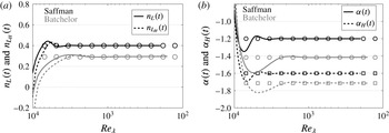
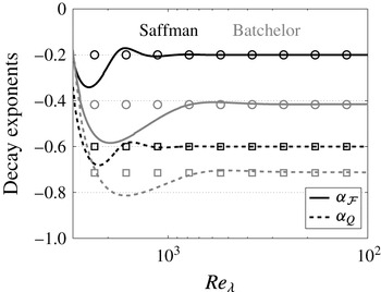
Decay laws for the kinetic (–) and helical (– –) fields, in Saffman (black) and Batchelor (grey) turbulence. Symbols refer to the theoretical predictions given in (4.1) for
 $\unicode[STIX]{x1D6FC}$
, (4.3) for
 $\unicode[STIX]{x1D6FC}_{H}$
and (4.2) for
 $L$
and
 $L_{H}$
. (a) Growth exponents of the kinetic and helical integral scales
 $L$
and
 $L_{H}$
. At a given
 $\unicode[STIX]{x1D70E}$
, the kinetic and helical theoretical exponents indicated by ○ cannot be distinguished. (b) Decay exponents of the kinetic energy and helicity
 $K$
and
 $K_{H}$
, where ○ and ▫ refer to the kinetic and helical theoretical predictions respectively.

Theoretical predictions for the kinetic and helical decay exponents
 $\unicode[STIX]{x1D6FC}$
and
 $\unicode[STIX]{x1D6FC}_{H}$
as a function of the infrared slope
 $\unicode[STIX]{x1D70E}$
.

4.2 Effect of helicity on the kinetic energy
$K(t)$
decay

The effects of helicity on the kinetic energy decay are firstly addressed. Simulations show that the decay exponent
 $\unicode[STIX]{x1D6FC}$
of the kinetic energy, where
 $K(t)\sim t^{\unicode[STIX]{x1D6FC}}$
, is not modified by helicity, except in the case of Batchelor turbulence (
 $\unicode[STIX]{x1D70E}=4$
), because of the reduction of the non-local inverse transfers analysed in § 3.2. Hence, one would expect the decay of
 $K(t)$
to be more rapid in Batchelor HHT than in Batchelor HIT: indeed, the non-local inverse transfers bring back less energy to the large scales. This is recovered in figure 5.
To analytically take into account the breakdown of the PLE hypothesis, a backscatter parameter
 $p$
is usually introduced (Lesieur & Ossia Reference Lesieur and Ossia2000; Meldi & Sagaut Reference Meldi and Sagaut2013; Briard et al.
Reference Briard, Gomez, Sagaut and Memari2015). In HIT, one has
 $p(\unicode[STIX]{x1D70E}=4)=0.55$
and
 $p(\unicode[STIX]{x1D70E}\leqslant 3)=0$
: in particular, in Batchelor HIT
 $K(t)\sim t^{-1.38}$
. Here, in Batchelor HHT,
 $K(t)\sim t^{-1.417}$
is obtained, and a least-square fit provides a new backscatter parameter
 $p_{H}=0.14$
for HHT. Consequently, with respect to HIT, only the backscatter parameter changes from
 $p$
to
 $p_{H}$
in HHT for the decay of kinetic energy
 $$\begin{eqnarray}\displaystyle K(t)\sim t^{\unicode[STIX]{x1D6FC}},\quad \unicode[STIX]{x1D6FC}=-2\frac{\unicode[STIX]{x1D70E}-p_{H}+1}{\unicode[STIX]{x1D70E}-p_{H}+3},\quad \left\{\begin{array}{@{}l@{}}p_{H}(\unicode[STIX]{x1D70E}=4)=0.14\quad \\ p_{H}(\unicode[STIX]{x1D70E}\leqslant 3)=0.\quad \end{array}\right. & & \displaystyle\end{eqnarray}$$
These decay exponents for the kinetic energy, whose values are gathered in table 2, are assessed in figure 5 in Saffman and Batchelor turbulence: only the case
 $\unicode[STIX]{x1D70E}=4$
differs from HIT, where here in HHT the decay of
 $K(t)$
is slightly more rapid. The fact that helicity does not influence much the energy cascade once the turbulence is fully developed is in good agreement with conclusions drawn by Polifke (Reference Polifke1991), Borue & Orszag (Reference Borue and Orszag1997).
4.3 The decay of helicity
$K_{H}(t)$

In the previous part, helicity was shown to impact the kinetic energy decay only in Batchelor turbulence. The emphasis is now put on the decay of
 $K_{H}$
itself. The method to predict the decay of helicity is similar to the one of an advected passive scalar, and even more simple. Indeed, as revealed in figure 4 and explained in § 3.2, the helical spectrum
 $H(k,t)$
experiences no strong back transfers, so that the PLE hypothesis is verified, from
 $\unicode[STIX]{x1D70E}=1$
to
 $\unicode[STIX]{x1D70E}=4$
. Therefore, there is no need to introduce a backscatter parameter. It is recalled that given the initial conditions (2.33), the spectral infrared slope of
 $H(k,t)$
is
 $\unicode[STIX]{x1D70E}_{H}=\unicode[STIX]{x1D70E}+1$
, where
 $\unicode[STIX]{x1D70E}$
is the infrared slope of
 $E(k,t)$
.
Then, it is reasonable to assume that the kinetic and helical integral scales
 $L(t)$
and
 $L_{H}(t)$
decay similarly, so that their algebraic exponents
 $n_{L}$
and
 $n_{L_{H}}$
are equal
 $$\begin{eqnarray}\displaystyle L_{(H)}(t)\sim t^{n_{L_{(H)}}},\quad n_{L_{H}}=\frac{2}{\unicode[STIX]{x1D70E}+3}\simeq n_{L}=\frac{2}{\unicode[STIX]{x1D70E}-p_{H}+3}. & & \displaystyle\end{eqnarray}$$
This assumption is completely assessed in figure 5 in both Saffman and Batchelor turbulence (the same kind of hypothesis for the scalar integral scale is made when it comes to predicting the decay of the scalar variance). Then, using either the continuity of
 $H(k,t)$
in
 $k_{H}=1/L_{H}$
to determine the decay law for
 $\unicode[STIX]{x1D716}_{H}$
, or dimensional analysis with
 $K_{H}\sim K/L_{H}$
, or equation (3.4), one obtains
 $$\begin{eqnarray}\displaystyle K_{H}(t)\sim t^{\unicode[STIX]{x1D6FC}_{H}},\quad \unicode[STIX]{x1D6FC}_{H}=-2\frac{\unicode[STIX]{x1D70E}+2}{\unicode[STIX]{x1D70E}+3}. & & \displaystyle\end{eqnarray}$$
Theoretical values of this expression for
 $\unicode[STIX]{x1D6FC}_{H}$
, gathered in table 2, are in excellent agreement with simulations presented in figure 5 for Saffman and Batchelor turbulence: one can remark that the more
 $\unicode[STIX]{x1D70E}$
increases, the more
 $K_{H}$
decays rapidly, similarly to the dynamics of
 $K(t)$
. In addition, the decay exponent of
 $\unicode[STIX]{x1D716}_{H}$
is
 $\unicode[STIX]{x1D6FC}_{H}-1$
, according to (2.20). Interestingly, the theoretical decay exponent of
 $K_{H}$
is equivalent to the one of the scalar variance in HIT with an infrared slope
 $\unicode[STIX]{x1D70E}_{T}=\unicode[STIX]{x1D70E}+1$
without any backscatter. Finally, our predictions for
 $K_{H}$
are compared to those of Levshin & Chkhetiani (Reference Levshin and Chkhetiani2013) in appendix B.
In conclusion, the present theoretical predictions for the decay of helicity and kinetic energy have been assessed numerically. This is the first time such a result is proposed, with a careful attention to initial conditions and infrared dynamics.
4.4 Robustness of the decay exponents – altered infrared dynamics
In § 3.2, for kinetic energy and helical spectra scaling in
 $E=Bk^{\unicode[STIX]{x1D70E}}$
and
 $H=B_{H}k^{\unicode[STIX]{x1D70E}_{H}}$
in fully developed turbulence, the evolution equations of
 $B(t)$
and
 $B_{H}(t)$
were derived in (3.10)–(3.11) in the infrared range, assuming the dominance of inverse non-local transfers
 $T_{E}^{-}$
and
 $T_{H}^{-}$
on local ones. For the initial conditions (2.33) where
 $\unicode[STIX]{x1D70E}_{H}=\unicode[STIX]{x1D70E}+1$
, it was notably found that the permanence of large eddies holds for Batchelor turbulence (
 $\unicode[STIX]{x1D70E}=4$
).
Nevertheless, one can wonder if other initial conditions would produce a different infrared dynamics, and this could be relevant to test the robustness of the decay exponents
 $\unicode[STIX]{x1D6FC}$
and
 $\unicode[STIX]{x1D6FC}_{H}$
derived in the previous sections. One can remark that in (3.10), the term responsible for the backscatter of
 $E$
is the one where the
 $k^{()}$
factor vanishes. Thus, it is legitimate to wonder if in (3.11) one could have
 $4+\unicode[STIX]{x1D70E}-\unicode[STIX]{x1D70E}_{H}=0$
in order to obtain
 $d_{t}B_{H}\neq 0$
, and consequently to create backscatter for the helical spectrum. It is worth noting that
 $2+\unicode[STIX]{x1D70E}_{H}-\unicode[STIX]{x1D70E}=0$
is impossible in (3.10) because of the realizability condition (2.22).
In order to simplify this study, the maximal helicity condition
 $H=kE$
is kept, but the initial kinetic energy spectrum is now changed into a sharply peaked Gaussian one
 $$\begin{eqnarray}\displaystyle E(k,t=0)=C_{1}\exp \left(-\frac{1}{(C_{2})^{2}}\left[\ln \left(\frac{k}{k_{L}}\right)\right]^{2}\right), & & \displaystyle\end{eqnarray}$$
with
 $C_{1}$
so that one has a unit initial kinetic energy, and
 $C_{2}=0.1$
. After a few turnover times, the kinetic energy spectrum scales in
 $E\sim Bk^{4}$
in the infrared range (Lesieur & Ossia Reference Lesieur and Ossia2000). Unlike (2.33), the helical infrared slope
 $\unicode[STIX]{x1D70E}_{H}$
is now different from
 $\unicode[STIX]{x1D70E}+1$
. As a consequence of (3.11), it follows that
 $\unicode[STIX]{x1D70E}_{H}=8$
, and that the helical spectrum experiences backscatter with
 $$\begin{eqnarray}\displaystyle \unicode[STIX]{x1D70E}=4,\quad \frac{\text{d}B_{H}}{\text{d}t}=\frac{14}{15}B(t)\int _{k_{L}}^{\infty }\unicode[STIX]{x1D703}_{0pp}\frac{H(p)}{p^{2}}\,\text{d}p. & & \displaystyle\end{eqnarray}$$
The theoretical infrared scaling prediction
 $H\sim k^{8}$
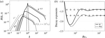
is assessed in figure 6, along with the
 $k^{4}$
infrared scaling of
 $E(k,t)$
: in this case, the permanence of large eddies is not verified anymore for
 $H(k,t)$
for the initial conditions (4.4). Nevertheless, it is shown in figure 6 as well that the previous theoretical decay exponents for kinetic energy and helicity are still valid, which implies that the backscatter of
 $H(k,t)$
is negligible in the decay. This case further illustrates the robustness of the theoretical predictions for the decay exponents.
(a) Helical spectrum
 $H(k,t)$
(black) for the initial condition (4.4) (– –) at various times
 $t/\unicode[STIX]{x1D70F}_{0}=10$
,
 $10^{3}$
and
 $10^{5}$
; the kinetic energy spectrum
 $E(k,t)$
is displayed as well (grey) at
 $t/\unicode[STIX]{x1D70F}_{0}=10^{5}$
. (b) Decay exponents
 $\unicode[STIX]{x1D6FC}$
(–) and
 $\unicode[STIX]{x1D6FC}_{H}$
(– –), where ○ and ▫ refer to the kinetic and helical theoretical predictions (4.1) and (4.3) respectively.

Simulations not presented here show that for Saffman turbulence (
 $E\sim k^{2}$
), a
 $k^{6}$
infrared scaling for
 $H$
could be created, but this is out of the maximal helicity framework:
 $H(k,t=0)$
should be Gaussian with
 $E(k,t=0)\sim k^{2}\exp (-k^{2})$
, and the theoretical decay exponents are still verified.
5 Helicity statistics in physical space
In the introduction, the main theoretical results for high Reynolds numbers HHT in physical space were recalled: notably two equivalent laws, found independently, which result from the conservation of helicity in inviscid flows. These two laws are the inertial scaling for the two-point triple velocity correlation (Chkhetiani Reference Chkhetiani1996)
 $$\begin{eqnarray}\displaystyle S(r)=\langle u_{L}u_{2}u_{3}^{\prime }\rangle =\frac{r^{2}}{30}\unicode[STIX]{x1D716}_{H}, & & \displaystyle\end{eqnarray}$$
and the inertial scaling for the third-order velocity–velocity–vorticity structure function (Gomez et al. Reference Gomez, Politano and Pouquet2000)
 $$\begin{eqnarray}\displaystyle D^{(uu\unicode[STIX]{x1D714})}(r)=\langle \unicode[STIX]{x1D6FF}u_{L}\unicode[STIX]{x1D6FF}u_{i}\unicode[STIX]{x1D6FF}\unicode[STIX]{x1D714}_{i}\rangle -{\textstyle \frac{1}{2}}\langle \unicode[STIX]{x1D6FF}u_{i}\unicode[STIX]{x1D6FF}u_{i}\unicode[STIX]{x1D6FF}\unicode[STIX]{x1D714}_{L}\rangle =-{\textstyle \frac{4}{3}}r\unicode[STIX]{x1D716}_{H}, & & \displaystyle\end{eqnarray}$$
where, as usual,
 $r$
is the distance between two points located in
 $\boldsymbol{x}$
and
 $\boldsymbol{x}^{\prime }=\boldsymbol{x}+\boldsymbol{r}$
, the
 $()_{L}$
refers to the component along
 $\boldsymbol{r}$
and the prime
 $^{\prime }$
to quantities expressed in
 $\boldsymbol{x}^{\prime }$
– which should not be confused with the prime of the correlation functions, such as
 $f^{\prime }(r)$
,
 $h^{\prime }(r)$
, which are the derivatives with respect to
 $r$
– and
 $\unicode[STIX]{x1D6FF}u_{i}=u_{i}^{\prime }-u_{i}$
.
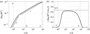
The latter law (5.2) is similar in its derivation to the laws for
 $\langle \unicode[STIX]{x1D6FF}u_{L}\unicode[STIX]{x1D6FF}q^{2}\rangle$
and
 $\langle \unicode[STIX]{x1D6FF}u_{L}\unicode[STIX]{x1D6FF}\unicode[STIX]{x1D703}^{2}\rangle$
in HIT, which come from the conservation of kinetic energy and scalar variance respectively in inviscid flows, where
 $\unicode[STIX]{x1D6FF}q^{2}=\unicode[STIX]{x1D6FF}u_{i}\unicode[STIX]{x1D6FF}u_{i}$
and
 $\unicode[STIX]{x1D703}$
is a fluctuating passive scalar field (Antonia et al.
Reference Antonia, Ould-Rouis, Anselmet and Zhu1997). These two scalings for HIT are well known and have been assessed numerous times, mostly using DNS (Yeung, Xu & Sreenivasan Reference Yeung, Xu and Sreenivasan2002; Watanabe & Gotoh Reference Watanabe and Gotoh2004; Yeung, Donzis & Sreenivasan Reference Yeung, Donzis and Sreenivasan2005; Bos et al.
Reference Bos, Chevillard, Scott and Rubinstein2012; Gotoh & Watanabe Reference Gotoh and Watanabe2015): a numerical validation using high Reynolds EDQNM simulations is proposed in appendix C to underline the analogy between transport of helicity, kinetic energy and scalar variance.
In this section, formulae that allow us to compute helical structure functions from spectral quantities are derived, similarly to what is usually done for velocity and scalar statistics in HIT (Monin, Yaglom & Lumley Reference Monin, Yaglom and Lumley2007). This further permits, using the EDQNM model presented in the previous sections, to assess numerically at high Reynolds numbers the two laws (5.1) and (5.2). In continuity of these developments in physical space, the evolution equation of the helical dissipation rate
 $\unicode[STIX]{x1D716}_{H}$
is addressed:
 $\unicode[STIX]{x1D716}_{H}$
itself and its production term are simplified, similarly to what is usually done for the kinetic energy dissipation rate in HIT. These analytical considerations provide further insights on the derivatives of helical correlations and skew-isotropic tensors, and lead to the definition of helical Taylor scale and derivative skewness.
5.1 Inertial scaling for
$S(r)$
and
$D^{(uu\unicode[STIX]{x1D714})}(r)$


This part aims at recalling the main steps of the derivation of the laws (5.1) and (5.2), and linking
 $S(r)$
and
 $D^{(uu\unicode[STIX]{x1D714})}(r)$
. The two-point second-order Reynolds tensor reads in HHT
 $$\begin{eqnarray}\displaystyle \unicode[STIX]{x1D619}_{ij}(r)=\langle u_{i}u_{j}^{\prime }\rangle =u^{2}\left[f(r)\unicode[STIX]{x1D6FF}_{ij}+\frac{r}{2}f^{\prime }(r)\left(\unicode[STIX]{x1D6FF}_{ij}-\frac{r_{i}r_{j}}{r^{2}}\right)\right]+\frac{h(r)}{r}\unicode[STIX]{x1D716}_{ijl}r_{l}, & & \displaystyle\end{eqnarray}$$
where
 $f=\langle u_{L}u_{L}^{\prime }\rangle /u^{2}$
is the second-order longitudinal correlation, with
 $u^{2}=2K/3$
and
 $h(r)=R_{23}(r)$
. The mixed velocity–vorticity correlation is given by
 $$\begin{eqnarray}\displaystyle \unicode[STIX]{x1D619}_{ij}^{H}=\langle u_{i}\unicode[STIX]{x1D714}_{j}^{\prime }\rangle =\unicode[STIX]{x1D716}_{jln}\frac{\unicode[STIX]{x2202}\unicode[STIX]{x1D619}_{in}}{\unicode[STIX]{x2202}x_{l}^{\prime }}=u^{2}\unicode[STIX]{x1D716}_{ijl}\left(\frac{r_{l}}{r}f^{\prime }+\frac{r_{l}}{2}f^{\prime \prime }\right)-2\unicode[STIX]{x1D6FF}_{ij}\frac{h}{r}+\left(\frac{h}{r}-h^{\prime }\right)\left(\unicode[STIX]{x1D6FF}_{ij}-\frac{r_{i}r_{j}}{r^{2}}\right). & & \displaystyle\end{eqnarray}$$
Also,
 $$\begin{eqnarray}\displaystyle \unicode[STIX]{x1D619}_{ii}^{H}(r)=-4\frac{h}{r}-2h^{\prime },\quad h(r)=-\frac{1}{3}rK_{H}. & & \displaystyle\end{eqnarray}$$
The latter expression shows that
 $h(0)=0$
. Then, the two-point triple velocity correlation contains an additional antisymmetric part with respect to HIT, so that (Chkhetiani Reference Chkhetiani1996; Gomez et al.
Reference Gomez, Politano and Pouquet2000)
 $$\begin{eqnarray}\displaystyle \langle u_{i}u_{j}u_{k}^{\prime }\rangle =\frac{k-rk^{\prime }}{2r^{3}}r_{i}r_{j}r_{k}-\unicode[STIX]{x1D6FF}_{ij}\frac{k}{2r}r_{k}+\frac{2k+rk^{\prime }}{4r}(\unicode[STIX]{x1D6FF}_{ik}r_{j}+\unicode[STIX]{x1D6FF}_{jk}r_{i})+S(r)\frac{r_{l}}{r^{2}}(\unicode[STIX]{x1D716}_{ikl}r_{j}+\unicode[STIX]{x1D716}_{jkl}r_{i}), & & \displaystyle\end{eqnarray}$$
where
 $k(r)=\langle u_{L}u_{L}u_{L}^{\prime }\rangle$
and
 $S(r)=\langle u_{L}u_{2}u_{3}^{\prime }\rangle$
: in particular,
 $\langle u_{2}u_{3}{u_{L}}^{\prime }\rangle =0$
and
 $\langle u_{L}u_{3}u_{2}^{\prime }\rangle =-S(r)$
, which gives
 $S(0)=0$
. Thus, from the evolution equation of
 $\unicode[STIX]{x1D619}_{ij}(r)$
 $$\begin{eqnarray}\displaystyle \frac{\unicode[STIX]{x2202}\unicode[STIX]{x1D619}_{ij}}{\unicode[STIX]{x2202}t}=\frac{\unicode[STIX]{x2202}}{\unicode[STIX]{x2202}r_{l}}(\langle u_{i}u_{l}u_{j}^{\prime }\rangle +\langle u_{j}u_{l}u_{i}^{\prime }\rangle )+2\unicode[STIX]{x1D708}\frac{\unicode[STIX]{x2202}^{2}\unicode[STIX]{x1D619}_{ij}}{\unicode[STIX]{x2202}r_{l}\unicode[STIX]{x2202}r_{l}}, & & \displaystyle\end{eqnarray}$$
it is possible to compute the evolution equation of the antisymmetric part
 $(\unicode[STIX]{x1D619}_{ij}-\unicode[STIX]{x1D619}_{ji})/2=h\unicode[STIX]{x1D716}_{ijl}r_{l}/r$
linked to helicity (Chkhetiani Reference Chkhetiani1996; Kurien Reference Kurien2003). The spatial derivative
 $\unicode[STIX]{x2202}_{r_{j}}$
erases the part which contains the third-order longitudinal correlation
 $k(r)$
, so that, after some algebra and using
 $\unicode[STIX]{x2202}_{t}K_{H}=-\unicode[STIX]{x1D716}_{H}$
, one obtains
 $$\begin{eqnarray}\displaystyle \frac{r}{3}\unicode[STIX]{x1D716}_{H}=\frac{2}{r^{3}}\frac{\unicode[STIX]{x2202}}{\unicode[STIX]{x2202}r}(r^{3}S)+2\unicode[STIX]{x1D708}\left(-\frac{2}{r^{2}}h(r)+\frac{2}{r}\frac{\unicode[STIX]{x2202}h}{\unicode[STIX]{x2202}r}+\frac{\unicode[STIX]{x2202}^{2}h}{\unicode[STIX]{x2202}r^{2}}\right). & & \displaystyle\end{eqnarray}$$
Further, neglecting the viscous effects in the inertial range and integrating over
 $r$
, one obtains (5.1). Then, it is possible to derive the equation for
 $D^{(uu\unicode[STIX]{x1D714})}$
starting from
 $$\begin{eqnarray}\displaystyle & \displaystyle \frac{\unicode[STIX]{x2202}\unicode[STIX]{x1D6FF}u_{i}}{\unicode[STIX]{x2202}t}+\unicode[STIX]{x1D6FF}u_{j}\frac{\unicode[STIX]{x2202}}{\unicode[STIX]{x2202}r_{j}}(\unicode[STIX]{x1D6FF}u_{i})=2\unicode[STIX]{x1D708}\frac{\unicode[STIX]{x2202}^{2}}{\unicode[STIX]{x2202}r_{j}\unicode[STIX]{x2202}r_{j}}(\unicode[STIX]{x1D6FF}u_{i}), & \displaystyle\end{eqnarray}$$
 $$\begin{eqnarray}\displaystyle & \displaystyle \frac{\unicode[STIX]{x2202}\unicode[STIX]{x1D6FF}\unicode[STIX]{x1D714}_{i}}{\unicode[STIX]{x2202}t}+\unicode[STIX]{x1D6FF}u_{j}\frac{\unicode[STIX]{x2202}}{\unicode[STIX]{x2202}r_{j}}(\unicode[STIX]{x1D6FF}\unicode[STIX]{x1D714}_{i})=\unicode[STIX]{x1D6FF}\unicode[STIX]{x1D714}_{j}\frac{\unicode[STIX]{x2202}}{\unicode[STIX]{x2202}r_{j}}(\unicode[STIX]{x1D6FF}u_{i})+2\unicode[STIX]{x1D708}\frac{\unicode[STIX]{x2202}^{2}}{\unicode[STIX]{x2202}r_{j}\unicode[STIX]{x2202}r_{j}}(\unicode[STIX]{x1D6FF}u_{i}), & \displaystyle\end{eqnarray}$$
where
 $\unicode[STIX]{x2202}/\unicode[STIX]{x2202}_{x_{j}^{\prime }}=\unicode[STIX]{x2202}/\unicode[STIX]{x2202}_{r_{j}}=-\unicode[STIX]{x2202}/\unicode[STIX]{x2202}_{x_{j}}$
has been used (see Antonia et al. (Reference Antonia, Ould-Rouis, Anselmet and Zhu1997) for further details on the method). Combining these two equations yields
 $$\begin{eqnarray}\displaystyle & & \displaystyle \frac{\unicode[STIX]{x2202}\langle \unicode[STIX]{x1D6FF}u_{i}\unicode[STIX]{x1D6FF}\unicode[STIX]{x1D714}_{i}\rangle }{\unicode[STIX]{x2202}t}+\frac{\unicode[STIX]{x2202}}{\unicode[STIX]{x2202}r_{j}}\left(\langle \unicode[STIX]{x1D6FF}u_{j}\unicode[STIX]{x1D6FF}u_{i}\unicode[STIX]{x1D6FF}\unicode[STIX]{x1D714}_{i}\rangle -\frac{1}{2}\langle \unicode[STIX]{x1D6FF}u_{i}\unicode[STIX]{x1D6FF}u_{i}\unicode[STIX]{x1D6FF}\unicode[STIX]{x1D714}_{j}\rangle \right)\nonumber\\ \displaystyle & & \displaystyle \quad =2\unicode[STIX]{x1D708}\frac{\unicode[STIX]{x2202}^{2}\langle \unicode[STIX]{x1D6FF}u_{i}\unicode[STIX]{x1D6FF}\unicode[STIX]{x1D714}_{i}\rangle }{\unicode[STIX]{x2202}r_{j}\unicode[STIX]{x2202}r_{j}}-4\underbrace{\unicode[STIX]{x1D708}\left\langle \frac{\unicode[STIX]{x2202}\unicode[STIX]{x1D6FF}u_{i}}{\unicode[STIX]{x2202}r_{j}}\frac{\unicode[STIX]{x2202}\unicode[STIX]{x1D6FF}\unicode[STIX]{x1D714}_{i}}{\unicode[STIX]{x2202}r_{j}}\right\rangle }_{=\unicode[STIX]{x1D716}_{H}}.\end{eqnarray}$$
Then,
 $\langle \unicode[STIX]{x1D6FF}u_{j}\unicode[STIX]{x1D6FF}u_{i}\unicode[STIX]{x1D6FF}\unicode[STIX]{x1D714}_{i}\rangle =r_{j}\langle \unicode[STIX]{x1D6FF}u_{L}\unicode[STIX]{x1D6FF}u_{i}\unicode[STIX]{x1D6FF}\unicode[STIX]{x1D714}_{i}\rangle /r$
, and
 $\unicode[STIX]{x2202}_{r_{j}}(D^{(uu\unicode[STIX]{x1D714})}r_{j}/r)=\unicode[STIX]{x2202}_{r}(r^{2}D^{(uu\unicode[STIX]{x1D714})})/r^{2}$
. Further neglecting the time derivative and the viscous term in the inertial range, integration over
 $r$
yields (5.2).
Interestingly, equations (5.1) and (5.2) can be linked: remarking that
 $\langle \unicode[STIX]{x1D6FF}u_{i}\unicode[STIX]{x1D6FF}\unicode[STIX]{x1D714}_{i}\rangle =2\langle u_{i}\unicode[STIX]{x1D714}_{i}\rangle -2\langle u_{i}\unicode[STIX]{x1D714}_{i}^{\prime }\rangle$
,
 $\unicode[STIX]{x2202}_{t}R_{11}^{H}=-2\unicode[STIX]{x1D716}_{H}/3$
, with
 $R_{11}^{H}=-2h/r$
, this provides
 $$\begin{eqnarray}\displaystyle \frac{1}{r^{2}}\frac{\unicode[STIX]{x2202}}{\unicode[STIX]{x2202}r}(r^{3}R_{11}^{H})=\langle u_{i}\unicode[STIX]{x1D714}_{i}^{\prime }\rangle =\unicode[STIX]{x1D619}_{ii}^{H},\quad \frac{1}{r}\frac{\unicode[STIX]{x2202}}{\unicode[STIX]{x2202}r}\left(\frac{1}{r^{2}}\frac{\unicode[STIX]{x2202}(r^{3}R_{11}^{H})}{\unicode[STIX]{x2202}r}\right)=\frac{1}{r^{4}}\frac{\unicode[STIX]{x2202}}{\unicode[STIX]{x2202}r}\left(r^{4}\frac{\unicode[STIX]{x2202}R_{11}^{H}}{\unicode[STIX]{x2202}r}\right),\quad & & \displaystyle\end{eqnarray}$$
and one gets by identification
 $$\begin{eqnarray}\displaystyle D^{(uu\unicode[STIX]{x1D714})}=\langle \unicode[STIX]{x1D6FF}u_{L}\unicode[STIX]{x1D6FF}u_{i}\unicode[STIX]{x1D6FF}\unicode[STIX]{x1D714}_{i}\rangle -\frac{1}{2}\langle \unicode[STIX]{x1D6FF}u_{i}\unicode[STIX]{x1D6FF}u_{i}\unicode[STIX]{x1D6FF}\unicode[STIX]{x1D714}_{L}\rangle =-\frac{8}{r^{3}}\frac{\unicode[STIX]{x2202}}{\unicode[STIX]{x2202}r}(r^{3}S(r)). & & \displaystyle\end{eqnarray}$$
This important relation is used in the next part, where (5.1) and (5.2) are assessed numerically at large Reynolds numbers.
5.2 Numerical assessment of
$S(r)$
and
$D^{(uu\unicode[STIX]{x1D714})}(r)$


Now that the main theoretical results have been recalled, the relations linking spectral quantities to helical structure functions are derived. First, one needs to obtain the evolution equations of
 $\langle u_{i}\unicode[STIX]{x1D714}_{i}^{\prime }\rangle /2$
: this is done starting from (5.8) since
 $$\begin{eqnarray}\displaystyle \frac{\langle u_{i}\unicode[STIX]{x1D714}_{i}^{\prime }\rangle }{2}=-\frac{1}{r^{2}}\frac{\unicode[STIX]{x2202}(r^{2}h)}{\unicode[STIX]{x2202}r},\quad \frac{r\unicode[STIX]{x1D716}_{H}}{3}=\frac{\unicode[STIX]{x2202}h}{\unicode[STIX]{x2202}t}. & & \displaystyle\end{eqnarray}$$
One obtains
 $$\begin{eqnarray}\displaystyle \frac{\unicode[STIX]{x2202}}{\unicode[STIX]{x2202}t}\left(\frac{\langle u_{i}\unicode[STIX]{x1D714}_{i}^{\prime }\rangle }{2}\right)=-\frac{2}{r^{2}}\frac{\unicode[STIX]{x2202}}{\unicode[STIX]{x2202}r}\left(\frac{1}{r}\frac{\unicode[STIX]{x2202}}{\unicode[STIX]{x2202}r}(r^{3}S)\right)-\frac{2\unicode[STIX]{x1D708}}{r^{4}}\frac{\unicode[STIX]{x2202}}{\unicode[STIX]{x2202}r}\left(r^{4}\frac{\unicode[STIX]{x2202}^{2}h}{\unicode[STIX]{x2202}r^{2}}\right). & & \displaystyle\end{eqnarray}$$
This equation needs to be identified with the helical Lin equation (2.32), so that
 $$\begin{eqnarray}\displaystyle -\frac{2}{r^{2}}\frac{\unicode[STIX]{x2202}}{\unicode[STIX]{x2202}r}\left(\frac{1}{r}\frac{\unicode[STIX]{x2202}}{\unicode[STIX]{x2202}r}(r^{3}S(r))\right)=\int _{0}^{\infty }S_{H}^{NL}(k)\frac{\sin (kr)}{kr}\,\text{d}k. & & \displaystyle\end{eqnarray}$$
After some algebra, one obtains
 $$\begin{eqnarray}\displaystyle & \displaystyle S(r)=\frac{1}{2}\int _{0}^{\infty }\frac{S_{H}^{NL}}{k^{2}}\left[\frac{\sin (kr)}{kr}-3\frac{\sin (kr)}{(kr)^{3}}+3\frac{\cos (kr)}{(kr)^{2}}\right]\,\text{d}k, & \displaystyle\end{eqnarray}$$
 $$\begin{eqnarray}\displaystyle & \displaystyle D^{(uu\unicode[STIX]{x1D714})}(r)=4\int _{0}^{\infty }\frac{S_{H}^{NL}}{k}\left[\frac{\sin (kr)}{(kr)^{2}}-\frac{\cos (kr)}{kr}\right]\,\text{d}k. & \displaystyle\end{eqnarray}$$
Notice that these two formulae are valid for both decaying and forced HHT, and the latter expression for
 $D^{(uu\unicode[STIX]{x1D714})}$
is very similar to the ones for
 $\langle \unicode[STIX]{x1D6FF}u_{L}\unicode[STIX]{x1D6FF}q^{2}\rangle$
and
 $\langle \unicode[STIX]{x1D6FF}u_{L}\unicode[STIX]{x1D6FF}\unicode[STIX]{x1D703}^{2}\rangle$
which can be found in appendix C, which is expected since they all refer to conservation laws. The relevance of the two previous formulae (5.17) and (5.18) is illustrated in figure 7, where the compensated helical third-order correlations
 $-D^{(uu\unicode[STIX]{x1D714})}/(r\unicode[STIX]{x1D716}_{H})$
and
 $S/(r^{2}\unicode[STIX]{x1D716}_{H})$
are displayed at high Reynolds numbers. The theoretical values
 $4/3$
and
 $1/30$
are almost recovered at
 $Re_{\unicode[STIX]{x1D706}}=3\times 10^{4}$
: the slight difference is comparable to the difference observed for the
 $-4/5$
law in decaying turbulence (Bos et al.
Reference Bos, Chevillard, Scott and Rubinstein2012). Interestingly,
 $D^{(uu\unicode[STIX]{x1D714})}$
is slightly closer to
 $4/3$
than
 $\langle \unicode[STIX]{x1D6FF}u_{L}\unicode[STIX]{x1D6FF}q^{2}\rangle$
in HHT. Simulations not presented here revealed that at the same high Reynolds numbers,
 $-\langle \unicode[STIX]{x1D6FF}u_{L}\unicode[STIX]{x1D6FF}q^{2}\rangle /(\unicode[STIX]{x1D716}r)$
is as close to
 $4/3$
in HIT and in HHT. Let us mention that an equivalent scaling for
 $S$
(the
 $2/15$
law) was already assessed in DNS (Kurien et al.
Reference Kurien, Taylor and Matsumoto2004b
). But so far, to our knowledge, the scaling for
 $D^{(uu\unicode[STIX]{x1D714})}$
was not verified numerically, at least for freely decaying turbulence: the present simulations show a very good agreement between EDQNM results and the theoretical expectations. Finally, it is revealed in figure 7 that
 $S\sim r^{4}$
at small scales, which is straightforward using (5.13), unlike
 $\langle \unicode[STIX]{x1D6FF}u_{L}^{3}\rangle$
,
 $\langle \unicode[STIX]{x1D6FF}u_{L}\unicode[STIX]{x1D6FF}q^{2}\rangle$
,
 $\langle \unicode[STIX]{x1D6FF}u_{L}\unicode[STIX]{x1D6FF}\unicode[STIX]{x1D703}^{2}\rangle$
and
 $D^{(uu\unicode[STIX]{x1D714})}$
which scale with
 $r^{3}$
(see figures 12 and 13).
Third-order helical correlations
 $D^{(uu\unicode[STIX]{x1D714})}$
and
 $S$
, for
 $\unicode[STIX]{x1D70E}=2$
at
 $Re_{\unicode[STIX]{x1D706}}=3\times 10^{4}$
, along with the integral and Kolmogorov scales
 $L$
and
 $\unicode[STIX]{x1D702}$
. (a)
 $-D^{(uu\unicode[STIX]{x1D714})}/(r\unicode[STIX]{x1D716}_{H})$
and
 $-\langle \unicode[STIX]{x1D6FF}u_{L}\unicode[STIX]{x1D6FF}q^{2}\rangle /(r\unicode[STIX]{x1D716})$
; (b)
 $S/(r^{2}\unicode[STIX]{x1D716}_{H})$
. (c) Different scalings of
 $D^{(uu\unicode[STIX]{x1D714})}$
and
 $S$
: the scale
 $\unicode[STIX]{x1D706}_{H}$
is defined later on in (5.24).

5.3 Evolution equation of
$\unicode[STIX]{x1D716}_{H}$

In this part, the evolution equation of the helicity dissipation rate is addressed. The objective is to simplify this equation, in a manner similar to what is usually done for the kinetic energy dissipation rate
 $\unicode[STIX]{x1D716}$
in HIT (Pope Reference Pope2000). More precisely,
 $\unicode[STIX]{x1D716}_{H}$
itself and its production term are greatly simplified, and expressed as simple functions of the derivatives of the fluctuating velocity and vorticity fields. The final expressions (5.22) and (5.31) constitute one of the main new theoretical contributions of the present work, and applications are proposed as well. The calculations being rather lengthy, the intermediate steps are gathered in appendix D for the sake of clarity. The evolution equation of
 $\unicode[STIX]{x1D716}_{H}$
reads
 $$\begin{eqnarray}\displaystyle & \displaystyle \frac{\unicode[STIX]{x2202}}{\unicode[STIX]{x2202}t}\left(\frac{\unicode[STIX]{x1D716}_{H}}{\unicode[STIX]{x1D708}}\right)+D[u,\unicode[STIX]{x1D714}]=-2\unicode[STIX]{x1D708}\left\langle \frac{\unicode[STIX]{x2202}^{2}u_{i}}{\unicode[STIX]{x2202}x_{j}\unicode[STIX]{x2202}x_{l}}\frac{\unicode[STIX]{x2202}^{2}\unicode[STIX]{x1D714}_{i}}{\unicode[STIX]{x2202}x_{j}\unicode[STIX]{x2202}x_{l}}\right\rangle , & \displaystyle\end{eqnarray}$$
 $$\begin{eqnarray}\displaystyle & \displaystyle D[u,\unicode[STIX]{x1D714}]=\left\langle \frac{\unicode[STIX]{x2202}u_{i}}{\unicode[STIX]{x2202}x_{j}}\frac{\unicode[STIX]{x2202}u_{l}}{\unicode[STIX]{x2202}x_{j}}\frac{\unicode[STIX]{x2202}\unicode[STIX]{x1D714}_{i}}{\unicode[STIX]{x2202}x_{l}}\right\rangle +\left\langle \frac{\unicode[STIX]{x2202}u_{i}}{\unicode[STIX]{x2202}x_{l}}\frac{\unicode[STIX]{x2202}u_{l}}{\unicode[STIX]{x2202}x_{j}}\frac{\unicode[STIX]{x2202}\unicode[STIX]{x1D714}_{i}}{\unicode[STIX]{x2202}x_{j}}\right\rangle -\left\langle \frac{\unicode[STIX]{x2202}u_{i}}{\unicode[STIX]{x2202}x_{j}}\frac{\unicode[STIX]{x2202}u_{i}}{\unicode[STIX]{x2202}x_{l}}\frac{\unicode[STIX]{x2202}\unicode[STIX]{x1D714}_{l}}{\unicode[STIX]{x2202}x_{j}}\right\rangle , & \displaystyle\end{eqnarray}$$
where the production term
 $D[u,\unicode[STIX]{x1D714}]$
contains contributions from spatial derivatives of skew-isotropic tensors such as
 $\langle u_{i}u_{j}\unicode[STIX]{x1D714}_{l}^{\prime }\rangle$
and
 $\langle \unicode[STIX]{x1D714}_{i}u_{j}u_{l}^{\prime }\rangle$
. In the two following subsections, both
 $\unicode[STIX]{x1D716}_{H}$
and
 $D[u,\unicode[STIX]{x1D714}]$
are simplified. This procedure consists into two steps: first, expressing
 $\unicode[STIX]{x1D716}_{H}$
and
 $D[u,\unicode[STIX]{x1D714}]$
as functions of the derivatives of
 $h(r)$
and
 $S(r)$
respectively; and then expressing these derivatives as functions of particular components of the fluctuating velocity and vorticity fields. Obviously, this is much more lengthy for
 $D[u,\unicode[STIX]{x1D714}]$
since it is a third-order moment, composed of three different terms. All results of this part remain valid whether the turbulence is forced or decaying.
5.3.1 Derivatives of
$\unicode[STIX]{x1D619}_{ij}^{H}(r)$
– determination of
$\unicode[STIX]{x1D716}_{H}$


The first step to simplify
 $\unicode[STIX]{x1D716}_{H}$
consists of expressing it as a function of the derivatives of
 $h(r)$
. To do so, one first needs to know the derivatives of
 $\unicode[STIX]{x1D619}_{ij}^{H}$
, analogously to what George & Hussein (Reference George and Hussein1991) did for
 $\unicode[STIX]{x1D716}$
in axisymmetric turbulence. One has,
 $$\begin{eqnarray}\displaystyle \frac{\unicode[STIX]{x2202}^{2}\unicode[STIX]{x1D619}_{ij}^{H}}{\unicode[STIX]{x2202}r_{p}\unicode[STIX]{x2202}r_{q}}=-\!\left\langle \frac{\unicode[STIX]{x2202}u_{i}}{\unicode[STIX]{x2202}x_{p}}\frac{\unicode[STIX]{x2202}\unicode[STIX]{x1D714}_{j}^{\prime }}{\unicode[STIX]{x2202}x_{q}^{\prime }}\right\rangle ,\quad \frac{\unicode[STIX]{x1D716}_{H}}{\unicode[STIX]{x1D708}}=-\!\left(\frac{\unicode[STIX]{x2202}^{2}\unicode[STIX]{x1D619}_{ii}^{H}}{\unicode[STIX]{x2202}r_{j}\unicode[STIX]{x2202}r_{j}}\right)_{r=0}=\left\langle \frac{\unicode[STIX]{x2202}u_{i}}{\unicode[STIX]{x2202}x_{j}}\frac{\unicode[STIX]{x2202}\unicode[STIX]{x1D714}_{i}}{\unicode[STIX]{x2202}x_{j}}\right\rangle . & & \displaystyle\end{eqnarray}$$
After some algebra gathered in appendix D, one gets the general expression of
 $\unicode[STIX]{x2202}_{pq}^{2}\unicode[STIX]{x1D619}_{ij}^{H}$
, from which one can obtain some relations between the derivatives of
 $h(r)$
. Then, using a Taylor expansion of
 $h(r)$
for
 $r\rightarrow 0$
(with
 $h(0)=0$
) yields the important theoretical result
 $$\begin{eqnarray}\displaystyle \unicode[STIX]{x1D716}_{H}=10\unicode[STIX]{x1D708}h^{\prime \prime \prime }(0)=15\unicode[STIX]{x1D708}\left\langle \frac{\unicode[STIX]{x2202}u_{1}}{\unicode[STIX]{x2202}x_{1}}\frac{\unicode[STIX]{x2202}\unicode[STIX]{x1D714}_{1}}{\unicode[STIX]{x2202}x_{1}}\right\rangle , & & \displaystyle\end{eqnarray}$$
where the prime
 $^{\prime }$
denotes a spatial derivative
 $\unicode[STIX]{x2202}/\unicode[STIX]{x2202}r$
. This expression permits to determine the helicity dissipation rate with one term instead of nine, and is equivalent to
 $\unicode[STIX]{x1D716}=15\unicode[STIX]{x1D708}\langle (\unicode[STIX]{x2202}_{1}u_{1})^{2}\rangle$
for the kinetic energy dissipation rate in HIT.
The natural application of the previous calculations for the dissipation rate of helicity is the definition of a helical Taylor scale
 $\unicode[STIX]{x1D706}_{H}$
. Its expression is found analogously to what is usually done for the longitudinal Taylor scale
 $\unicode[STIX]{x1D706}$
(Pope Reference Pope2000), i.e. considering the osculating curve
 $P_{H}(r)$
of
 $h(r)$
in
 $r=0$
, which reads
 $$\begin{eqnarray}\displaystyle P_{H}(r)=h(0)+rh^{\prime }(0)+\frac{r^{2}}{2}h^{\prime \prime }(0)+\frac{r^{3}}{6}h^{\prime \prime \prime }(0)=-r\frac{K_{H}}{3}+r^{3}\frac{\unicode[STIX]{x1D716}_{H}}{60\unicode[STIX]{x1D708}}, & & \displaystyle\end{eqnarray}$$
and
 $\unicode[STIX]{x1D706}_{H}$
is further defined by
 $P_{H}(\unicode[STIX]{x1D706}_{H})=0$
and
 $\unicode[STIX]{x1D706}_{H}\neq 0$
, which yields
 $$\begin{eqnarray}\displaystyle \unicode[STIX]{x1D706}_{H}=\sqrt{\frac{20\unicode[STIX]{x1D708}K_{H}}{\unicode[STIX]{x1D716}_{H}}}. & & \displaystyle\end{eqnarray}$$
It is worth noting that this new expression obtained by analytical considerations is analogous to the classical one for the velocity
 $\unicode[STIX]{x1D706}=\sqrt{20\unicode[STIX]{x1D708}K/\unicode[STIX]{x1D716}}$
. The relevance of this formula is illustrated in figure 8. Both
 $\unicode[STIX]{x1D706}$
and
 $\unicode[STIX]{x1D706}_{H}$
are displayed, at large and moderate Reynolds numbers for Saffman turbulence. Both scales indicate the beginning of a region where viscous dissipation balances nonlinear transfers. At high Reynolds numbers,
 $\unicode[STIX]{x1D706}$
and
 $\unicode[STIX]{x1D706}_{H}$
cannot be distinguished, whereas
 $\unicode[STIX]{x1D706}_{H}$
is a bit smaller at moderate Reynolds numbers. The wavenumber
 $k_{\unicode[STIX]{x1D702}}^{H}$
, defined in (3.1) and proposed by Ditlevsen & Giuliani (Reference Ditlevsen and Giuliani2001), is presented as well: it seems to have a similar physical meaning as
 $\unicode[STIX]{x1D706}_{H}$
, at least at large Reynolds numbers, and some explanations are provided in appendix E. Moreover, figure 8 illustrates the viscous production of helicity, already observed in figure 2 where the helical spectrum was negative around
 $k_{\unicode[STIX]{x1D702}}$
: indeed,
 $-2\unicode[STIX]{x1D708}k^{3}H$
is positive near
 $k_{\unicode[STIX]{x1D702}}$
here. Finally,
 $\unicode[STIX]{x1D706}_{H}$
is displayed as well in figure 7, and is located at scales larger than the separation between the
 $r$
and
 $r^{3}$
scalings for
 $D^{(uu\unicode[STIX]{x1D714})}$
.
Taylor scales for kinetic energy and helicity
 $\unicode[STIX]{x1D706}$
and
 $\unicode[STIX]{x1D706}_{H}$
, along with the corresponding spectral viscous fluxes
 $-2\unicode[STIX]{x1D708}k^{3}E$
and
 $-2\unicode[STIX]{x1D708}k^{3}H$
and the nonlinear transfers
 $kS_{E}^{NL}$
and
 $kS_{H}^{NL}$
for
 $\unicode[STIX]{x1D70E}=2$
. The wavenumbers
 $k_{\unicode[STIX]{x1D702}}^{H}$
(3.1) and
 $k_{\unicode[STIX]{x1D702}}$
are displayed as well. The black curves are for the kinetic field, and the grey ones for the helical one. (a)
 $Re_{\unicode[STIX]{x1D706}}=10^{4}$
. (b)
 $Re_{\unicode[STIX]{x1D706}}=400$
.

A secondary application of these calculations is to express analytically the impact of helicity on the second-order longitudinal correlation
 $f(r\rightarrow 0)$
. Indeed, unlike HIT, where all odd derivatives of
 $f(r)$
for
 $r=0$
are zero, one can show that
 $f^{\prime \prime \prime }(0)$
is a priori different from zero in HHT (one has always
 $f^{\prime }(0)=0$
because of homogeneity). Expressing
 $\unicode[STIX]{x2202}_{11}^{2}R_{23}^{H}$
and
 $\unicode[STIX]{x2202}_{33}^{2}R_{23}^{H}$
thanks to (D 3) yields
 $$\begin{eqnarray}\displaystyle f^{\prime \prime \prime }(0)=-\frac{1}{2}\left\langle \frac{\unicode[STIX]{x2202}u_{2}}{\unicode[STIX]{x2202}x_{1}}\frac{\unicode[STIX]{x2202}\unicode[STIX]{x1D714}_{3}}{\unicode[STIX]{x2202}x_{1}}\right\rangle =-\!\left\langle \frac{\unicode[STIX]{x2202}u_{2}}{\unicode[STIX]{x2202}x_{3}}\frac{\unicode[STIX]{x2202}\unicode[STIX]{x1D714}_{3}}{\unicode[STIX]{x2202}x_{3}}\right\rangle , & & \displaystyle\end{eqnarray}$$
so that the Taylor expansion of
 $f(r)$
reads
 $$\begin{eqnarray}\displaystyle f(r)=1-\frac{r^{2}}{2}\frac{\unicode[STIX]{x1D716}}{15\unicode[STIX]{x1D708}u^{2}}\underbrace{+\frac{r^{3}}{6}f^{\prime \prime \prime }(0)}_{Additional\;HHT\;term}+\frac{r^{4}}{24}\frac{2P}{35u^{2}}, & & \displaystyle\end{eqnarray}$$
where
 $P=\int _{0}^{\infty }k^{4}E(k)\,\text{d}k$
is the palinstrophy.
5.3.2 Determination of the production term
$D[u,\unicode[STIX]{x1D714}]$

The procedure used to determine
 $\unicode[STIX]{x1D716}_{H}$
is now applied to the production term
 $D[u,\unicode[STIX]{x1D714}]$
: since this term is complex and involves derivatives of two different tensors
 $\langle u_{i}u_{j}\unicode[STIX]{x1D714}_{l}^{\prime }\rangle$
and
 $\langle \unicode[STIX]{x1D714}_{i}u_{j}u_{l}^{\prime }\rangle$
, the determination is divided into two steps. First,
 $D[u,\unicode[STIX]{x1D714}]$
is expressed as a function of the derivatives of
 $S(r)$
, and it will be shown that only
 $S^{(iv)}(0)$
remains. Then,
 $S^{(iv)}(0)$
is expressed as a function of the derivatives of the fluctuating velocity and vorticity fields.
As pointed out in Gomez et al. (Reference Gomez, Politano and Pouquet2000), the tensor
 $\langle \unicode[STIX]{x1D714}_{i}u_{j}u_{l}^{\prime }\rangle$
is much more complicated to handle than
 $\langle u_{i}u_{j}\unicode[STIX]{x1D714}_{l}^{\prime }\rangle$
, which can be linked easily to
 $\langle u_{i}u_{j}u_{l}^{\prime }\rangle$
given in (5.6)
 $$\begin{eqnarray}\displaystyle \unicode[STIX]{x1D719}_{ijl}^{(uu\unicode[STIX]{x1D714})}=\langle u_{i}u_{j}\unicode[STIX]{x1D714}_{l}^{\prime }\rangle =\unicode[STIX]{x1D716}_{lpq}\frac{\unicode[STIX]{x2202}\langle u_{i}u_{j}u_{q}^{\prime }\rangle }{\unicode[STIX]{x2202}r_{p}},\quad \unicode[STIX]{x1D719}_{ijl}^{(\unicode[STIX]{x1D714}uu)}=\langle \unicode[STIX]{x1D714}_{i}u_{j}u_{l}^{\prime }\rangle . & & \displaystyle\end{eqnarray}$$
Calculations detailed in appendix D first permit us to link derivatives of
 $\unicode[STIX]{x1D719}_{ijl}^{(uu\unicode[STIX]{x1D714})}$
and
 $\unicode[STIX]{x1D719}_{ijl}^{(\unicode[STIX]{x1D714}uu)}$
to
 $D[u,\unicode[STIX]{x1D714}]$
according to
 $$\begin{eqnarray}\displaystyle D[u,\unicode[STIX]{x1D714}]=\left(\frac{\unicode[STIX]{x2202}^{3}}{\unicode[STIX]{x2202}r_{j}\unicode[STIX]{x2202}r_{j}\unicode[STIX]{x2202}r_{l}}[\unicode[STIX]{x1D719}_{ili}^{(uu\unicode[STIX]{x1D714})}+\unicode[STIX]{x1D719}_{ili}^{(\unicode[STIX]{x1D714}uu)}-\unicode[STIX]{x1D719}_{lii}^{(\unicode[STIX]{x1D714}uu)}]\right)_{r=0}, & & \displaystyle\end{eqnarray}$$
where the derivatives of
 $\unicode[STIX]{x1D719}_{ijl}^{(uu\unicode[STIX]{x1D714})}$
and
 $\unicode[STIX]{x1D719}_{ijl}^{(\unicode[STIX]{x1D714}uu)}$
contain derivatives of
 $S(r)$
. Taylor expansions of
 $S(r)$
for
 $r\rightarrow 0$
further give
 $$\begin{eqnarray}\displaystyle D[u,\unicode[STIX]{x1D714}]=\left\langle \frac{\unicode[STIX]{x2202}u_{i}}{\unicode[STIX]{x2202}x_{j}}\frac{\unicode[STIX]{x2202}u_{l}}{\unicode[STIX]{x2202}x_{j}}\frac{\unicode[STIX]{x2202}\unicode[STIX]{x1D714}_{i}}{\unicode[STIX]{x2202}x_{l}}\right\rangle +\left\langle \frac{\unicode[STIX]{x2202}u_{i}}{\unicode[STIX]{x2202}x_{l}}\frac{\unicode[STIX]{x2202}u_{l}}{\unicode[STIX]{x2202}x_{j}}\frac{\unicode[STIX]{x2202}\unicode[STIX]{x1D714}_{i}}{\unicode[STIX]{x2202}x_{j}}\right\rangle -\left\langle \frac{\unicode[STIX]{x2202}u_{i}}{\unicode[STIX]{x2202}x_{j}}\frac{\unicode[STIX]{x2202}u_{i}}{\unicode[STIX]{x2202}x_{l}}\frac{\unicode[STIX]{x2202}\unicode[STIX]{x1D714}_{l}}{\unicode[STIX]{x2202}x_{j}}\right\rangle =-35S^{(iv)}(0). & & \displaystyle\end{eqnarray}$$
Now that
 $D[u,\unicode[STIX]{x1D714}]$
has been linked to
 $S^{(iv)}(0)$
, the final step is to express the fourth derivative of
 $S(r)$
as derivatives of the fluctuating velocity and vorticity fields, so that
 $D[u,\unicode[STIX]{x1D714}]$
can be evaluated by DNS for instance. For this purpose, the explicit sixth-order tensor
 $\unicode[STIX]{x2202}_{npq}^{3}\unicode[STIX]{x1D719}_{ijl}^{(uu\unicode[STIX]{x1D714})}$
is needed, and is given in appendix D. From this lengthy expression, one notably gets
 $$\begin{eqnarray}\displaystyle \left(\frac{\unicode[STIX]{x2202}^{3}\unicode[STIX]{x1D719}_{111}^{(uu\unicode[STIX]{x1D714})}}{\unicode[STIX]{x2202}r_{1}^{3}}\right)_{r=0}=-S^{(iv)}(0), & & \displaystyle\end{eqnarray}$$
from which one finally obtains the second important result of this section
 $$\begin{eqnarray}\displaystyle D[u,\unicode[STIX]{x1D714}]=-35S^{(iv)}(0)=35\left\langle \frac{\unicode[STIX]{x2202}^{2}u_{1}^{2}}{\unicode[STIX]{x2202}x_{1}^{2}}\frac{\unicode[STIX]{x2202}\unicode[STIX]{x1D714}_{1}}{\unicode[STIX]{x2202}x_{1}}\right\rangle , & & \displaystyle\end{eqnarray}$$
which permits us notably to compute
 $D[u,\unicode[STIX]{x1D714}]$
with only one term, instead of eighty-one. Further proceeding as in Kerr (Reference Kerr1985), i.e. identifying (5.19) with the spectral evolution equation of
 $\unicode[STIX]{x1D716}_{H}$
 $$\begin{eqnarray}\displaystyle \frac{\unicode[STIX]{x2202}\unicode[STIX]{x1D716}_{H}}{\unicode[STIX]{x2202}t}=2\unicode[STIX]{x1D708}\int _{0}^{\infty }k^{2}S_{H}^{NL}(k,t)\,\text{d}k-4\unicode[STIX]{x1D708}^{2}\int _{0}^{\infty }k^{4}H(k,t)\,\text{d}k, & & \displaystyle\end{eqnarray}$$
provides
 $$\begin{eqnarray}\displaystyle S^{(iv)}(0)=\frac{2}{35}\int _{0}^{\infty }k^{2}S_{H}^{NL}(k,t)\,\text{d}k. & & \displaystyle\end{eqnarray}$$
Hence, one can define, analogously to the mixed-derivative skewness of a passive scalar in HIT, a helical-derivative skewness as
 $$\begin{eqnarray}\displaystyle S_{uu\unicode[STIX]{x1D714}} & = & \displaystyle \left.\left\langle \frac{\unicode[STIX]{x2202}^{2}u_{1}^{2}}{\unicode[STIX]{x2202}x_{1}^{2}}\frac{\unicode[STIX]{x2202}\unicode[STIX]{x1D714}_{1}}{\unicode[STIX]{x2202}x_{1}}\right\rangle \right/\left(\left\langle \frac{\unicode[STIX]{x2202}u_{1}}{\unicode[STIX]{x2202}x_{1}}\frac{\unicode[STIX]{x2202}\unicode[STIX]{x1D714}_{1}}{\unicode[STIX]{x2202}x_{1}}\right\rangle \sqrt{\left\langle \left(\frac{\unicode[STIX]{x2202}u_{1}}{\unicode[STIX]{x2202}x_{1}}\right)^{2}\right\rangle }\right)\end{eqnarray}$$
 $$\begin{eqnarray}\displaystyle & = & \displaystyle -\frac{3\sqrt{30}}{14}\frac{\displaystyle \int _{0}^{\infty }k^{2}S_{H}^{NL}\,\text{d}k}{\sqrt{\displaystyle \int _{0}^{\infty }k^{2}E\,\text{d}k}\displaystyle \int _{0}^{\infty }k^{2}H\,\text{d}k}.\end{eqnarray}$$
Interestingly, the factor
 $3\sqrt{30}/14$
is identical to the one of the velocity-derivative skewness in HIT.
The helical-derivative skewness
 $S_{uu\unicode[STIX]{x1D714}}$
is displayed in figure 9 as a function of the Reynolds number
 $Re_{\unicode[STIX]{x1D706}}$
. Only Saffman turbulence is presented, because the curve for Batchelor turbulence is identical at high Reynolds numbers, similarly to the velocity and mixed-derivative skewnesses in HIT. The initial oscillations at large
 $Re_{\unicode[STIX]{x1D706}}$
correspond to the first turnover times of the simulation, when the turbulence is not fully developed yet. As for the velocity and mixed-derivative skewnesses,
 $S_{uu\unicode[STIX]{x1D714}}$
is negative and reaches an asymptotic value at large Reynolds numbers
 $S_{uu\unicode[STIX]{x1D714}}^{\infty }=-0.141$
. This value
 $S_{uu\unicode[STIX]{x1D714}}^{\infty }$
is lower in magnitude than asymptotic values for the velocity and mixed derivative skewnesses in HIT which are approximately
 $\simeq -0.5$
. The knowledge of the helical-derivative skewness is of importance for two reasons: it is of theoretical interest since it permits us to have a strong analogy between the evolution equations of
 $\unicode[STIX]{x1D716}$
in HIT and
 $\unicode[STIX]{x1D716}_{H}$
in HHT. From a more practical point of view, the previous developments which led to
 $S_{uu\unicode[STIX]{x1D714}}$
show that there exists, in homogeneous helical turbulence, a quantity which is constant at large Reynolds numbers: such a result could be used to improve Reynolds averaged Navier–Stokes (RANS) models for helical flows, where the production term would be linked to
 $S_{uu\unicode[STIX]{x1D714}}$
.
Helical-derivative skewness
 $S_{uu\unicode[STIX]{x1D714}}(t)$
in HHT for
 $\unicode[STIX]{x1D70E}=2$
.

6 Effects of helicity in a turbulence with a mean scalar gradient
In this section, the transport of a passive scalar field
 $\unicode[STIX]{x1D703}$
is addressed. However, since there are no explicit contributions of helicity in the spectral scalar–scalar two-point correlation evolution equation, a vertical mean scalar gradient
 $\unicode[STIX]{x1D740}=(0,0,-\unicode[STIX]{x1D6EC})$
is added. In purely isotropic turbulence with a mean scalar gradient, the well-known cospectrum, scaling in
 ${\mathcal{F}}\sim \unicode[STIX]{x1D6EC}\unicode[STIX]{x1D716}^{-1/3}k^{-7/3}$
in the inertial range, appears. When both helicity and a mean scalar gradient are combined, a second spectrum is created, called the quadrature spectrum
 $Q(k,t)$
, linked to the imaginary antisymmetric part of the scalar flux
 $F_{i}(\boldsymbol{k})$
, or spectral two-point velocity–scalar correlation. This quadrature spectrum was reported in Mydlarski & Warhaft (Reference Mydlarski and Warhaft1998), and shown to be zero in non-helical turbulence with a mean scalar gradient in O’Gorman & Pullin (Reference O’Gorman and Pullin2005). Consequently, we choose here the framework of helical turbulence with a mean scalar gradient in order to create this quadrature spectrum and analyse its properties. In the two next parts, it is first proposed to derive the evolution equation of
 $Q(k,t)$
and its nonlinear transfer terms within the EDQNM framework, and secondly to investigate the inertial scaling of the quadrature spectrum. Analogies with the effects of helicity on the kinetic energy spectrum are pointed out, and the decay exponent of helicity along with the helical Taylor scale given in §§4 and 5.3 are used. A unit Prandtl number is considered, and simulations not presented here have revealed that the scalar variance spectrum still scales in
 $k^{-5/3}$
in the inertial range despite the presence of helicity.
6.1 Evolution equation of the quadrature spectrum
The scalar flux can be decomposed similarly to the spectral Reynolds tensor
 $\hat{\unicode[STIX]{x1D619}}_{ij}$
in (2.8), as
 $$\begin{eqnarray}\displaystyle F_{i}(\boldsymbol{k},t)=\frac{3}{2}E_{j}^{F}(k,t)P_{ij}(\boldsymbol{k})+\frac{3}{2}\text{i}\unicode[STIX]{x1D700}_{ijn}\unicode[STIX]{x1D6FC}_{n}\frac{E_{j}^{Q}(k,t)}{k}, & & \displaystyle\end{eqnarray}$$
where both
 $E_{j}^{F}$
and
 $E_{j}^{Q}$
are real. The first part of the decomposition is usual (see Briard et al. (Reference Briard, Gomez and Cambon2016) and references therein) and is linked to the cospectrum
 ${\mathcal{F}}$
when a mean scalar gradient is present
 $$\begin{eqnarray}\displaystyle {\mathcal{F}}(k,t)=4\unicode[STIX]{x03C0}k^{2}E_{3}^{F}(k,t)=\int _{S_{k}}F_{3}(\boldsymbol{k},t)\,\text{d}^{2}\boldsymbol{k}. & & \displaystyle\end{eqnarray}$$
Whereas the second part is linked to the quadrature spectrum
 $Q$
, which is non-zero in the presence of helicity
 $$\begin{eqnarray}\displaystyle Q(k,t)=4\unicode[STIX]{x03C0}k^{2}E_{3}^{Q}(k,t)=\int _{S_{k}}\text{i}\unicode[STIX]{x1D716}_{3jl}k_{l}F_{j}(\boldsymbol{k},t)\,\text{d}^{2}\boldsymbol{k}. & & \displaystyle\end{eqnarray}$$
The phenomenon creating this additional contribution to the scalar flux, parallel to the mean gradient in the presence of helicity, is called ‘skew diffusion’ in Moffatt & Tsinober (Reference Moffatt and Tsinober1992). It is worth noting that from the decomposition (6.1) and (6.3), imaginary components of the scalar flux, perpendicular to the mean scalar gradient, are non-zero. Nevertheless, these components vanish after spherical averaging.
The mixed vorticity–scalar correlation is then
 $\langle \unicode[STIX]{x1D714}_{3}\unicode[STIX]{x1D703}\rangle =\int _{0}^{\infty }Q(k,t)\,\text{d}k$
, and its evolution equation reads
 $$\begin{eqnarray}\displaystyle \frac{\unicode[STIX]{x2202}\langle \unicode[STIX]{x1D714}_{3}\unicode[STIX]{x1D703}\rangle }{\unicode[STIX]{x2202}t}=\frac{2}{3}\unicode[STIX]{x1D6EC}K_{H}+\left\langle \unicode[STIX]{x1D703}\unicode[STIX]{x1D714}_{j}\frac{\unicode[STIX]{x2202}u_{3}}{\unicode[STIX]{x2202}x_{j}}\right\rangle -(\unicode[STIX]{x1D708}+a)\left\langle \frac{\unicode[STIX]{x2202}\unicode[STIX]{x1D703}}{\unicode[STIX]{x2202}x_{j}}\frac{\unicode[STIX]{x2202}\unicode[STIX]{x1D714}_{3}}{\unicode[STIX]{x2202}x_{j}}\right\rangle . & & \displaystyle\end{eqnarray}$$
In the framework of homogeneous helical turbulence with a mean scalar gradient, the spherically averaged Lin equations for the cospectrum and the quadrature spectrum are
 $$\begin{eqnarray}\displaystyle & \displaystyle \left(\frac{\unicode[STIX]{x2202}}{\unicode[STIX]{x2202}t}+2\unicode[STIX]{x1D708}k^{2}\right){\mathcal{F}}(k,t)=\frac{2}{3}\unicode[STIX]{x1D6EC}E(k,t)+\underbrace{S_{3}^{F}(k,t)+S_{3}^{F(hel)}(k,t)}_{S_{F}^{NL}(k,t)}, & \displaystyle\end{eqnarray}$$
 $$\begin{eqnarray}\displaystyle & \displaystyle \left(\frac{\unicode[STIX]{x2202}}{\unicode[STIX]{x2202}t}+2\unicode[STIX]{x1D708}k^{2}\right)Q(k,t)=\frac{2}{3}\unicode[STIX]{x1D6EC}H(k,t)+S_{Q}^{NL}(k,t), & \displaystyle\end{eqnarray}$$
where helicity is the production term of the quadrature spectrum. The nonlinear transfer of the cospectrum
 $S_{3}^{F}$
is always present when there is a mean scalar gradient, whereas
 $S_{3}^{F(hel)}$
is the additional contribution arising from the presence of helicity
 $$\begin{eqnarray}\displaystyle & & \displaystyle S_{i}^{F(hel)}(k,t)=4\unicode[STIX]{x03C0}^{2}\int _{\unicode[STIX]{x1D6E5}_{k}}\unicode[STIX]{x1D703}_{kpq}^{F}k^{2}(x+yz){\mathcal{H}}^{\prime \prime }(2pzE_{i}^{Q}-kE_{i}^{Q^{\prime }})\,\text{d}p\,\text{d}q\nonumber\\ \displaystyle & & \displaystyle \quad +\,4\unicode[STIX]{x03C0}^{2}\int _{\unicode[STIX]{x1D6E5}_{k}}\unicode[STIX]{x1D703}_{pkq}^{F}k(x+yz)[{\mathcal{H}}(p^{2}E_{i}^{Q^{\prime \prime }}-q(q-2ky)E_{i}^{Q^{\prime }})-k^{2}{\mathcal{H}}^{\prime \prime }E_{i}^{Q^{\prime }}]\,\text{d}p\,\text{d}q,\end{eqnarray}$$
where
 $\unicode[STIX]{x1D703}_{kpq}^{F}$
is the characteristic relaxation time of the triple velocity–velocity–scalar correlations, given in Briard et al. (Reference Briard, Gomez and Cambon2016). The remarkable feature is that
 $S_{3}^{F(hel)}$
is a conservative transfer, with zero integral over the whole wavenumber space, similarly to
 $S^{(hel)}$
in the evolution equation of
 $E(k,t)$
. The spherically averaged quadrature nonlinear transfer
 $S_{Q}^{NL}=S_{3}^{Q}$
finally reads
 $$\begin{eqnarray}\displaystyle & & \displaystyle S_{i}^{Q}(k,t)=4\unicode[STIX]{x03C0}^{2}\int _{\unicode[STIX]{x1D6E5}_{k}}\unicode[STIX]{x1D703}_{kpq}^{F}k^{3}pq[\!{\mathcal{E}}_{0}^{\prime \prime }(E_{i}^{Q^{\prime }}(xyz+2z^{2}-y^{2})-2z(xy+z)E_{i}^{Q})\nonumber\\ \displaystyle & & \displaystyle \quad +\,z(xy+z){\mathcal{H}}^{\prime \prime }(2E_{i}^{F}-E_{i}^{F^{\prime }})\!]\,\text{d}p\,\text{d}q\nonumber\\ \displaystyle & & \displaystyle \quad +\,4\unicode[STIX]{x03C0}^{2}\int _{\unicode[STIX]{x1D6E5}_{k}}\unicode[STIX]{x1D703}_{pkq}^{F}k^{2}q[\!kp{\mathcal{E}}_{0}^{\prime \prime }(E_{i}^{Q^{\prime }}(xyz+2z^{2}-y^{2})-2(1-y^{2})E_{i}^{Q})-kpz(xy+z){\mathcal{H}}^{\prime \prime }E_{i}^{F^{\prime }}\nonumber\\ \displaystyle & & \displaystyle \quad +\,k{\mathcal{E}}_{0}(E_{i}^{Q^{\prime \prime }}p(1-y^{2})-E_{i}^{Q^{\prime }}q(x-yz-2xy^{2}))\nonumber\\ \displaystyle & & \displaystyle \quad -\,pq{\mathcal{H}}(E_{i}^{F^{\prime \prime }}y(1-y^{2})+E_{i}^{F^{\prime }}(xz+y^{3}-y(1-x^{2})))\!]\,\text{d}p\,\text{d}q,\end{eqnarray}$$
and is not a conservative transfer, similarly to
 $S_{3}^{F}$
. Its integral over the whole wavenumber space yields, according to (6.4), the term
 $\langle \unicode[STIX]{x1D703}\unicode[STIX]{x1D714}_{j}\unicode[STIX]{x2202}_{j}u_{3}\rangle$
.
6.2 Decay of
$\langle \unicode[STIX]{x1D714}_{3}\unicode[STIX]{x1D703}\rangle$
and inertial scaling of
$Q(k,t)$


For these numerical simulations, the initial condition (2.33) is used, with
 $Q(k,t=0)={\mathcal{F}}(k,t=0)=0$
. First, the decay of
 $\langle \unicode[STIX]{x1D714}_{3}\unicode[STIX]{x1D703}\rangle$
is addressed. From the Lin equation (6.6) of
 $Q(k,t)$
, it follows that the decay exponent of
 $\langle \unicode[STIX]{x1D714}_{3}\unicode[STIX]{x1D703}\rangle$
is
 $\unicode[STIX]{x1D6FC}_{Q}=\unicode[STIX]{x1D6FC}_{H}+1$
, where
 $\unicode[STIX]{x1D6FC}_{H}$
is given in (4.3), because the production term linked to helicity is the one responsible for the creation of the quadrature spectrum. This yields
 $$\begin{eqnarray}\displaystyle \langle \unicode[STIX]{x1D714}_{3}\unicode[STIX]{x1D703}\rangle \sim t^{\unicode[STIX]{x1D6FC}_{Q}},\quad \unicode[STIX]{x1D6FC}_{Q}=-\frac{\unicode[STIX]{x1D70E}+1}{\unicode[STIX]{x1D70E}+3}. & & \displaystyle\end{eqnarray}$$
It is recalled that the decay exponent of
 $\langle u_{3}\unicode[STIX]{x1D703}\rangle$
is
 $\unicode[STIX]{x1D6FC}_{{\mathcal{F}}}=\unicode[STIX]{x1D6FC}+1$
, where the backscatter parameter
 $p_{H}=0.14$
of § 4 should be used for consistency. Both
 $\unicode[STIX]{x1D6FC}_{{\mathcal{F}}}$
and
 $\unicode[STIX]{x1D6FC}_{Q}$
are assessed for Saffman and Batchelor turbulence in figure 10 at large Reynolds numbers. For a given infrared slope
 $\unicode[STIX]{x1D70E}$
, the decay of
 $\langle \unicode[STIX]{x1D714}_{3}\unicode[STIX]{x1D703}\rangle$
is faster than
 $\langle u_{3}\unicode[STIX]{x1D703}\rangle$
, similarly to the decay of
 $K_{H}$
being faster than
 $K$
.
Decay exponents
 $\unicode[STIX]{x1D6FC}_{Q}$
and
 $\unicode[STIX]{x1D6FC}_{{\mathcal{F}}}$
of
 $\langle \unicode[STIX]{x1D714}_{3}\unicode[STIX]{x1D703}\rangle$
(– –) and
 $\langle u_{3}\unicode[STIX]{x1D703}\rangle$
(–) respectively, for
 $\unicode[STIX]{x1D70E}=2$
(black) and
 $\unicode[STIX]{x1D70E}=4$
(grey); theoretical predictions, ▫ for
 $\unicode[STIX]{x1D6FC}_{Q}$
(6.9), and ○ for
 $\unicode[STIX]{x1D6FC}_{{\mathcal{F}}}$
.

Regarding the nonlinear transfers: the impact of the quadrature spectrum on the cospectrum is rather weak and can be observed through the conservative nonlinear transfer
 $S_{3}^{F(hel)}$
. This transfer is linked to an inverse cascade of
 $\langle u_{3}\unicode[STIX]{x1D703}\rangle$
, localized at large scales, between the integral and the helical Taylor scales. This can be qualitatively compared to the impact of helicity on the kinetic energy spectrum dynamics through
 $S^{(hel)}$
in figure 3. One could conclude that helicity only slightly reduces the nonlinear transfers of the cospectrum at large scales. Then, the quadrature nonlinear transfer
 $S_{Q}^{NL}$
itself is similar to the cospectrum one
 $S_{3}^{F}$
, but less intense.
(a) Cospectrum and quadrature nonlinear transfers. (b) Cospectrum
 ${\mathcal{F}}(k,t)$
and quadrature spectrum
 $Q(k,t)$
;
 $-Q(k,t)$
is displayed in grey. Both for
 $\unicode[STIX]{x1D70E}=2$
at
 $Re_{\unicode[STIX]{x1D706}}=5\times 10^{3}$
, after a hundred turnover times, along with the integral, helical Taylor and Kolmogorov wavenumbers
 $k_{L}$
,
 $1/\unicode[STIX]{x1D706}_{H}$
and
 $k_{\unicode[STIX]{x1D702}}$
.

Finally, in figure 11, the quadrature spectrum itself is presented. In the infrared range, it scales like
 $Q\sim k^{3}$
for Saffman turbulence, because the helical spectrum itself evolves in
 $H\sim k^{3}$
: indeed, helicity, through the mean scalar gradient, is the production term of the quadrature spectrum. In the inertial range,
 $Q(k,t)$
is first positive for scales larger than the helical Taylor scale
 $\unicode[STIX]{x1D706}_{H}$
, and scales in
 $k^{-7/3}$
similarly to
 ${\mathcal{F}}$
. Whereas for scales smaller than
 $\unicode[STIX]{x1D706}_{H}$
, the spectral slope is close to
 $k^{-5/3}$
and the quadrature spectrum is negative: it is recalled that around
 $k_{\unicode[STIX]{x1D702}}$
,
 $H(k,t)$
is also negative.
One can propose theoretical inertial scalings for the quadrature spectrum. In the positive region, assuming in (6.6) that
 $\unicode[STIX]{x2202}_{t}Q\sim \unicode[STIX]{x1D6EC}H$
, with the classical characteristic inertial time
 $(k^{2}\unicode[STIX]{x1D716})^{-1/3}$
, this gives
 $$\begin{eqnarray}\displaystyle Q(k,t)\sim \unicode[STIX]{x1D6EC}\unicode[STIX]{x1D716}_{H}\unicode[STIX]{x1D716}^{-2/3}k^{-7/3},\quad k_{L}<k<\unicode[STIX]{x1D706}_{H}^{-1}. & & \displaystyle\end{eqnarray}$$
For the negative region of
 $Q(k,t)$
, the quadrature spectrum should only depend on
 $\unicode[STIX]{x1D716}_{H}$
since this is the negative small scales of
 $H(k,t)$
which are responsible for this inertial–helical range of
 $Q(k,t)$
. Thus, one gets
 $$\begin{eqnarray}\displaystyle Q(k,t)\sim \unicode[STIX]{x1D6EC}\unicode[STIX]{x1D716}_{H}^{1/3}k^{-5/3},\quad \unicode[STIX]{x1D706}_{H}^{-1}<k<k_{\unicode[STIX]{x1D702}}. & & \displaystyle\end{eqnarray}$$
This change of slope, from
 $k^{-7/3}$
for
 $k\unicode[STIX]{x1D706}_{H}<1$
, to
 $k^{-5/3}$
for
 $k\unicode[STIX]{x1D706}_{H}>1$
, observed in figure 11 and justified with dimensional and physical arguments, can also be interpreted in terms of a change in characteristic time scales, from
 $\unicode[STIX]{x1D70F}=(k^{2}\unicode[STIX]{x1D716})^{-1/3}$
to
 $\unicode[STIX]{x1D70F}_{H}=(k\unicode[STIX]{x1D716}_{H})^{-1/3}$
. The latter time scale was notably proposed by Kurien, Taylor & Matsumoto (Reference Kurien, Taylor and Matsumoto2004a
) for an alternative scaling of
 $H(k,t)$
at small scales. This characteristic time scale
 $\unicode[STIX]{x1D70F}_{H}$
is relevant for the inertial–helical scaling of
 $Q$
when it is negative. Indeed, for
 $k\unicode[STIX]{x1D706}_{H}>1$
, the equation (6.6) of
 $Q$
can be written
 $\unicode[STIX]{x2202}_{t}Q\sim S_{Q}^{NL}$
. For the nonlinear term, using the inertial scalings (3.2) for
 $H$
and
 ${\mathcal{F}}$
, along with
 $\unicode[STIX]{x1D703}_{kpq}^{F}\sim \unicode[STIX]{x1D70F}_{H}$
, gives
 $S_{Q}^{NL}\sim \unicode[STIX]{x1D6EC}k^{-4/3}\unicode[STIX]{x1D716}_{H}^{2/3}$
. Finally, one has
 $Q\sim \unicode[STIX]{x1D70F}_{H}S_{Q}^{NL}$
so that (6.11) is recovered.
As a conclusion, the combined effects of helicity and mean scalar gradient were investigated. Nonlinear transfer terms were derived for the evolution equations of the quadrature spectrum
 $Q(k,t)$
and of the cospectrum
 ${\mathcal{F}}(k,t)$
within the EDQNM framework. Fundamental properties of
 $Q(k,t)$
were tackled: a prediction for the decay of
 $\langle \unicode[STIX]{x1D714}_{3}\unicode[STIX]{x1D703}\rangle$
was proposed and assessed numerically,
 $Q(k,t)$
was found to slightly decrease the large-scale nonlinear transfers of
 ${\mathcal{F}}$
through helicity, and finally, the main theoretical result is that
 $Q(k,t)$
has two different scalings in the inertial range, which could be associated with two different characteristic time scales.
7 Conclusion
The classical framework of decaying homogeneous helical turbulence where mirror symmetry is broken (skew-isotropic turbulence) at large Reynolds numbers was addressed using an eddy-damped quasi-normal Markovian closure.
Some existing results were recovered here for decaying skew-isotropic turbulence, in order to validate the use of EDQNM for HHT, which could be summarized in three features. First, when helicity is initially present at large scales, helicity cascades towards small scales along with the kinetic energy, creating a
 $k^{-5/3}$
inertial range that extends up to the Kolmogorov wavenumber
 $k_{\unicode[STIX]{x1D702}}$
. The
 $k^{-5/3}$
scaling of the helical spectrum
 $H(k,t)$
is similar to the one of an advected passive scalar, also obtained with dimensional analysis by assuming that the inertial characteristic time
 $\unicode[STIX]{x1D70F}(k)=(k^{2}\unicode[STIX]{x1D716})^{-1/3}$
is identical for both the kinetic and helical fields. Secondly, in the early stage of the decay, helicity slows down the filling of the kinetic energy spectrum at small scales. Consequently, there is an initial reduction of the kinetic energy transfers: this is a transitory effect, since once the turbulence is fully developed, the effects of helicity on the kinetic energy decay are rather weak. Finally, two-point third-order helical correlations were investigated: notably, the ‘four-thirds’ law for helical structure functions, and the
 $1/30$
law for the helical correlation
 $S(r)$
, were assessed with EDQNM at very high Reynolds numbers in decaying turbulence. It is worth noting that the two formulae linking helical correlations in physical space and spectral nonlinear helical transfers are new results of this work.
Then, EDQNM simulations were used to assess some new theoretical predictions of fundamental interest for helical turbulence. First, the infrared dynamics of the kinetic energy and helical spectra was investigated theoretically using non-local expansions in the nonlinear transfers. It clearly appears that in Batchelor HHT, helicity reduces the back transfers of kinetic energy with respect to HIT: consequently, inverse non-local transfers are weakened and bring back less energy to large scales. Furthermore, the permanence of large eddies is shown to be verified for
 $H(k,t)$
, even in Batchelor turbulence, with classical initial conditions such that the kinetic and helical infrared slopes are
 $\unicode[STIX]{x1D70E}_{H}=\unicode[STIX]{x1D70E}+1$
. These two features are assessed numerically with EDQNM. An original configuration, with different initial conditions, also exhibited a
 $k^{8}$
infrared scaling for
 $H(k,t)$
, along with some helical backscatter.
Secondly, as a direct application of the previous infrared dynamics analysis, the impact of helicity on the long-time kinetic energy decay was shown to be quite subtle: indeed, the decay of
 $K(t)$
is not modified with regard to HIT, except in the case of Batchelor turbulence (
 $E(k<k_{L},t=0)\sim k^{4}$
) where it is slightly accelerated, because of the less-intense inverse transfers. In addition, in agreement with dimensional analysis, theoretical decay exponents for helicity were derived, and assessed numerically at large Reynolds numbers: in particular, it is found that helicity decays faster than the kinetic energy.
Thirdly, the evolution equation of the helicity dissipation rate
 $\unicode[STIX]{x1D716}_{H}$
was studied, with a particular attention on the derivatives of second- and third-order skew-isotropic tensors such as
 $\langle u_{i}\unicode[STIX]{x1D714}_{j}^{\prime }\rangle$
,
 $\langle u_{i}u_{j}\unicode[STIX]{x1D714}_{l}^{\prime }\rangle$
and
 $\langle \unicode[STIX]{x1D714}_{i}u_{j}u_{l}^{\prime }\rangle$
. As an important result of these analytical developments,
 $\unicode[STIX]{x1D716}_{H}$
itself is expressed as a function of
 $h^{\prime \prime \prime }(0)$
only, where
 $h=R_{23}(r)$
, and its production term
 $D[u,\unicode[STIX]{x1D714}]$
as a function of
 $S^{(iv)}(0)$
only, where
 $S=\langle u_{L}u_{2}u_{3}^{\prime }\rangle$
. It follows that
 $\unicode[STIX]{x1D716}_{H}$
and
 $D[u,\unicode[STIX]{x1D714}]$
can be expressed with only one term, instead of nine and eighty-one respectively.
Fourthly, as a direct application of these fundamental results, a helical Taylor scale was defined
 $\unicode[STIX]{x1D706}_{H}=\sqrt{20\unicode[STIX]{x1D708}K_{H}/\unicode[STIX]{x1D716}_{H}}$
, whose expression is analogous to the longitudinal Taylor scale
 $\unicode[STIX]{x1D706}$
for kinetic energy. Such a scale is new for the helicity field, and its relevance was illustrated numerically:
 $\unicode[STIX]{x1D706}_{H}$
is the scale from which viscous dissipation of helicity becomes dynamically important, and at large Reynolds numbers, it is very close to
 $\unicode[STIX]{x1D706}$
. Moreover, a helical-derivative skewness was defined as well, similarly to the velocity derivative and mixed-derivative skewnesses in HIT, negative and constant at large Reynolds numbers.
Finally, it was shown that combining a mean scalar gradient and helicity produces the quadrature spectrum
 $Q(k,t)$
, linked to the imaginary antisymmetric part of the scalar flux. As a consequence, the large-scale nonlinear transfers of the cospectrum are slightly reduced. After deriving the nonlinear transfer terms within the EDQNM framework, the main finding for
 $Q(k,t)$
is that it has two different scalings in the inertial range: for
 $k\unicode[STIX]{x1D706}_{H}<1$
,
 $Q\sim k^{-7/3}$
, and then for
 $k\unicode[STIX]{x1D706}_{H}>1$
,
 $Q\sim k^{-5/3}$
: this change in the spectral slope can be interpreted as the characteristic time evolving from
 $(k^{2}\unicode[STIX]{x1D716})^{-1/3}$
to
 $(k\unicode[STIX]{x1D716}_{H})^{-1/3}$
at smaller scales.
In conclusion, the present work thoroughly validates on the one hand the use of EDQNM for the study of homogeneous helical turbulence, and brings new important insights about the fundamental properties of helicity in high Reynolds numbers turbulent flows on the other hand. As stated in the introduction, the next step would be to combine effects of helicity with other mechanisms such as shear, stratification, rotation and mean temperature gradient.
Appendix A. Details of non-local expansions
The non-local inverse kinetic and helical transfers
 $T_{E}^{-}$
and
 $T_{H}^{-}$
, given in (3.7) and (3.9), are obtained after performing non-local expansions of their associated fluxes. Some details are provided here, and are inspired by the calculations of Lesieur & Schertzer (Reference Lesieur and Schertzer1978).
First, one needs to define the non-local parameter
 $a=r-1$
, that marks the limit between local and non-local transfers, where
 $r=10^{1/17}$
has been defined in § 2.4 and depends on the discretization.
Separating the local and non-local contributions, the Lin equation of the kinetic energy spectrum reads
 $$\begin{eqnarray}\displaystyle \left(\frac{\unicode[STIX]{x2202}}{\unicode[STIX]{x2202}t}+2\unicode[STIX]{x1D708}k^{2}\right)E(k,t)=\underbrace{S_{E}^{NL}}_{Local}(k,t)+\underbrace{T_{E}^{\pm }}_{Non\text{-}local}(k,t), & & \displaystyle\end{eqnarray}$$
where the non-local transfer is linked to the non-local flux through
 $$\begin{eqnarray}\displaystyle T_{E}^{\pm }(k,t)=-\frac{\unicode[STIX]{x2202}}{\unicode[STIX]{x2202}k}(\unicode[STIX]{x1D6F1}^{+}-\unicode[STIX]{x1D6F1}^{-}). & & \displaystyle\end{eqnarray}$$
 $\unicode[STIX]{x1D6F1}^{+}$
and
 $\unicode[STIX]{x1D6F1}^{-}$
are respectively the non-local fluxes of kinetic energy toward very small and very large scales. Since we are interested in the infrared dynamics, we focus only on the inverse non-local flux
 $\unicode[STIX]{x1D6F1}^{-}$
, given by
 $$\begin{eqnarray}\displaystyle & \displaystyle \unicode[STIX]{x1D6F1}^{-}(k,t)=2\int _{0}^{k}\,\text{d}k^{\prime }\int _{\mathit{sup}(k,k^{\prime }/a)}^{\infty }\,\text{d}p\int _{p-k^{\prime }}^{p}S(k^{\prime },p,q)\,\text{d}q, & \displaystyle\end{eqnarray}$$
 $$\begin{eqnarray}\displaystyle & \displaystyle S^{(iso)}(k,t)=\int _{\unicode[STIX]{x1D6E5}_{k}}\underbrace{\unicode[STIX]{x1D703}_{kpq}\frac{(xy+z^{3})}{q}E(q)(k^{2}E(p)-p^{2}E(k))}_{S(k,p,q)}\,\text{d}p\,\text{d}q. & \displaystyle\end{eqnarray}$$
These inverse non-local transfers are such that
 $k\ll p\sim q$
, so that the small parameter considered in the expansion is
 $\unicode[STIX]{x1D701}=k/p\ll 1$
. This yields, after some algebra
 $$\begin{eqnarray}\displaystyle \unicode[STIX]{x1D6F1}^{-}(k,t) & = & \displaystyle \frac{14}{15}\int _{0}^{k}{k^{\prime }}^{4}\left[\int _{\mathit{sup}(k,k^{\prime }/a)}^{\infty }\unicode[STIX]{x1D703}_{k^{\prime }pp}\frac{E(p)^{2}}{p^{2}}\text{d}p\right]\,\text{d}k^{\prime }\nonumber\\ \displaystyle & & \displaystyle -\,\frac{2}{15}\int _{0}^{k}{k^{\prime }}^{2}E(k^{\prime })\left[\int _{\mathit{sup}(k,k^{\prime }/a)}^{\infty }\unicode[STIX]{x1D703}_{k^{\prime }pp}\left(5E(p)+p\frac{\unicode[STIX]{x2202}E}{\unicode[STIX]{x2202}p}\right)\text{d}p\right]\,\text{d}k^{\prime }.\end{eqnarray}$$
The derivation of
 $\unicode[STIX]{x1D6F1}^{-}$
at the lowest order in
 $k/k_{L}$
yields (3.5). Similarly, expanding
 $S^{(hel)}$
when
 $k\ll p\sim q$
, one obtains the inverse non-local helical flux
 $$\begin{eqnarray}\displaystyle \unicode[STIX]{x1D6F1}^{(hel)-}(k,t) & = & \displaystyle -\frac{14}{15}\int _{0}^{k}{k^{\prime }}^{4}\int _{\mathit{sup}(k,k^{\prime }/a)}^{\infty }\unicode[STIX]{x1D703}_{k^{\prime }pp}\frac{H(p)^{2}}{p^{4}}\,\text{d}p\,\text{d}k^{\prime }\end{eqnarray}$$
 $$\begin{eqnarray}\displaystyle & & \displaystyle +\,\frac{2}{15}\int _{0}^{k}{k^{\prime }}^{2}H(k^{\prime })\int _{\mathit{sup}(k,k^{\prime }/a)}^{\infty }\frac{\unicode[STIX]{x1D703}_{k^{\prime }pp}}{p^{2}}\left(9H(p)-p\frac{\unicode[STIX]{x2202}H}{\unicode[STIX]{x2202}p}\right)\,\text{d}p\,\text{d}k^{\prime }.\end{eqnarray}$$
The spatial derivative of
 $\unicode[STIX]{x1D6F1}^{(hel)-}$
yields (3.6). The procedure is similar for the expansion of
 $S_{H}^{NL}$
, and one gets
 $$\begin{eqnarray}\displaystyle \unicode[STIX]{x1D6F1}_{H}^{-}(k,t) & = & \displaystyle \unicode[STIX]{x1D6F1}_{H1}^{-}(k,t)+\unicode[STIX]{x1D6F1}_{H2}^{-}(k,t)=\frac{14}{15}\int _{0}^{k}{k^{\prime }}^{4}\int _{\mathit{sup}(k,k^{\prime }/a)}^{\infty }\unicode[STIX]{x1D703}_{k^{\prime }pp}\frac{H(p)E(p)}{p^{4}}\,\text{d}p\,\text{d}k^{\prime }\nonumber\\ \displaystyle & & \displaystyle -\,\frac{2}{15}\int _{0}^{k}{k^{\prime }}^{2}H(k^{\prime })\int _{\mathit{sup}(k,k^{\prime }/a)}^{\infty }\unicode[STIX]{x1D703}_{k^{\prime }pp}\left(5E(p)+p\frac{\unicode[STIX]{x2202}E}{\unicode[STIX]{x2202}p}\right)\,\text{d}p\,\text{d}k^{\prime }\nonumber\\ \displaystyle & & \displaystyle -\,\frac{14}{15}\int _{0}^{k}{k^{\prime }}^{4}\int _{\mathit{sup}(k,k^{\prime }/a)}^{\infty }\unicode[STIX]{x1D703}_{k^{\prime }pp}\frac{H(p)E(p)}{p^{4}}\,\text{d}p\,\text{d}k^{\prime }\nonumber\\ \displaystyle & & \displaystyle +\,\frac{14}{15}\int _{0}^{k}{k^{\prime }}^{4}E(k^{\prime })\int _{\mathit{sup}(k,k^{\prime }/a)}^{\infty }\unicode[STIX]{x1D703}_{k^{\prime }pp}\frac{H(p)}{p^{2}}\,\text{d}p\,\text{d}k^{\prime }.\end{eqnarray}$$
One can note that the first and third terms cancel each other, which explains that there is no strong
 $k^{4}$
non-local inverse transfer for
 $H$
. Then, the derivation of
 $\unicode[STIX]{x1D6F1}_{H}^{-}$
gives (3.9).
Similar calculations can be performed for a weakly diffusive passive scalar field, for non-local transfers from large to very small scales, as done in Briard et al. (Reference Briard, Gomez, Sagaut and Memari2015).
Appendix B.
$\unicode[STIX]{x1D6FC}_{H}$
: comparison with Levshin & Chkhetiani (Reference Levshin and Chkhetiani2013)

The present theoretical predictions (4.3) for the decay exponent of helicity
 $\unicode[STIX]{x1D6FC}_{H}$
are compared to those of Levshin & Chkhetiani (Reference Levshin and Chkhetiani2013) (hereafter LC13) in table 3, obtained with considerations of integral invariants. To fill in table 3, a very reasonable assumption is made, since initial conditions are not defined in LC13, so that there is no infrared slope
 $\unicode[STIX]{x1D70E}$
. Hence, when in LC13 a decay exponent for the kinetic energy is proposed, it is associated here with its corresponding infrared slope according to the CBC theory:
 $K\sim t^{-1}\rightarrow \unicode[STIX]{x1D70E}=1$
,
 $K\sim t^{-6/5}\rightarrow \unicode[STIX]{x1D70E}=2$
,
 $K\sim t^{-4/3}\rightarrow \unicode[STIX]{x1D70E}=3$
, and
 $K\sim t^{-10/7}\rightarrow \unicode[STIX]{x1D70E}=4$
(backscatter is not taken into account in LC13). The values of
 $\unicode[STIX]{x1D6FC}_{H}$
from LC13 are the same as the ones coming from (4.3) (
 $-3/2$
,
 $-8/5$
,
 $-5/3$
and
 $-12/7$
), but there are not associated with the correct infrared slopes. For instance in Saffman turbulence (
 $K(t)\sim t^{-6/5}$
and
 $\unicode[STIX]{x1D70E}=2$
), two laws are proposed in LC13 for helicity:
 $K_{H}^{LC13}(t)\sim t^{-3/2}$
and
 $K_{H}^{LC13}(t)\sim t^{-5/3}$
. This is impossible: using our theoretical prediction (4.3),
 $K_{H}^{LC13}(t)\sim t^{-3/2}$
corresponds to
 $\unicode[STIX]{x1D70E}=1$
, and
 $K_{H}^{LC13}(t)\sim t^{-5/3}$
to
 $\unicode[STIX]{x1D70E}=3$
, whereas
 $K(t)\sim t^{-6/5}$
corresponds to
 $\unicode[STIX]{x1D70E}=2$
.
Consequently, it seems that the results of LC13 correspond to infrared slopes of
 $E$
and
 $H$
chosen independently, without respecting the realizability condition (2.22) which fixes the helical slope once and for all, as soon as an infrared slope is chosen for
 $E$
: equation (2.22) forbids initial conditions such as
 $\unicode[STIX]{x1D70E}_{H}=\unicode[STIX]{x1D70E}$
and
 $\unicode[STIX]{x1D70E}_{H}=\unicode[STIX]{x1D70E}-1$
.
Comparison of the different theoretical decay exponents
 $\unicode[STIX]{x1D6FC}_{H}$
of helicity, obtained with classical CBC-like arguments, and by LC13, as a function of the infrared slope
 $\unicode[STIX]{x1D70E}$
of the kinetic energy spectrum
 $E(k,t)$
.

Appendix C. Third-order structure functions in HIT
In this section, third-order structure functions for velocity and scalar fields are briefly investigated in HIT, to illustrate the analogy with helicity in HHT. The so-called ‘four-thirds’ laws for
 $\langle \unicode[STIX]{x1D6FF}u_{L}\unicode[STIX]{x1D6FF}q^{2}\rangle$
and
 $\langle \unicode[STIX]{x1D6FF}u_{L}\unicode[STIX]{x1D6FF}\unicode[STIX]{x1D703}^{2}\rangle$
are recalled, along with the formulae which allow us to compute them from the spherically averaged nonlinear kinetic and scalar transfers. Multiplying the evolution equation of
 $\unicode[STIX]{x1D6FF}u_{i}$
(5.9) by
 $2\unicode[STIX]{x1D6FF}u_{i}$
and using ensemble average yields
 $$\begin{eqnarray}\displaystyle \frac{\unicode[STIX]{x2202}}{\unicode[STIX]{x2202}t}\langle \unicode[STIX]{x1D6FF}q^{2}\rangle +\frac{\unicode[STIX]{x2202}}{\unicode[STIX]{x2202}r_{j}}\langle \unicode[STIX]{x1D6FF}u_{j}\unicode[STIX]{x1D6FF}q^{2}\rangle =2\unicode[STIX]{x1D708}\frac{\unicode[STIX]{x2202}^{2}}{\unicode[STIX]{x2202}r_{j}\unicode[STIX]{x2202}r_{j}}\langle \unicode[STIX]{x1D6FF}q^{2}\rangle -4\underbrace{\unicode[STIX]{x1D708}\left\langle \frac{\unicode[STIX]{x2202}\unicode[STIX]{x1D6FF}u_{i}}{\unicode[STIX]{x2202}r_{j}}\frac{\unicode[STIX]{x2202}\unicode[STIX]{x1D6FF}u_{i}}{\unicode[STIX]{x2202}r_{j}}\right\rangle }_{=\unicode[STIX]{x1D716}}. & & \displaystyle\end{eqnarray}$$
The pressure contribution is zero because
 $\unicode[STIX]{x2202}_{x_{j}^{\prime }}=\unicode[STIX]{x2202}_{r_{j}}=-\unicode[STIX]{x2202}_{x_{j}}$
. Further neglecting the time derivative and writing
 $-4\unicode[STIX]{x1D716}=-4/3\unicode[STIX]{x2202}_{r_{j}}(\unicode[STIX]{x1D716}r_{j})$
, one gets
 $$\begin{eqnarray}\displaystyle \langle \unicode[STIX]{x1D6FF}u_{j}\unicode[STIX]{x1D6FF}q^{2}\rangle =2\unicode[STIX]{x1D708}\frac{\unicode[STIX]{x2202}}{\unicode[STIX]{x2202}r_{j}}\langle \unicode[STIX]{x1D6FF}q^{2}\rangle -\frac{4}{3}\unicode[STIX]{x1D716}r_{j}, & & \displaystyle\end{eqnarray}$$
where the result of von Kármán & Howarth (Reference von Kármán and Howarth1938) has been used (
 $2\unicode[STIX]{x1D719}/r+\unicode[STIX]{x1D719}^{\prime }=0\Leftrightarrow \unicode[STIX]{x1D719}=0$
) combined with
 $\unicode[STIX]{x2202}^{2}/(\unicode[STIX]{x2202}r_{j}\unicode[STIX]{x2202}r_{j})=(2/r\unicode[STIX]{x2202}_{r}+\unicode[STIX]{x2202}_{rr}^{2})$
. At high Reynolds numbers in the inertial range, this eventually gives
 $$\begin{eqnarray}\displaystyle \langle \unicode[STIX]{x1D6FF}u_{L}\unicode[STIX]{x1D6FF}q^{2}\rangle (r)=-{\textstyle \frac{4}{3}}\unicode[STIX]{x1D716}r, & & \displaystyle\end{eqnarray}$$
with the usual convention
 $r_{1}=r$
, and
 $r_{2}=r_{3}=0$
. It is possible to make a link between (C 3) and the ‘four-fifths’ law
 $$\begin{eqnarray}\displaystyle \langle \unicode[STIX]{x1D6FF}u_{L}^{3}\rangle =-{\textstyle \frac{4}{5}}\unicode[STIX]{x1D716}r. & & \displaystyle\end{eqnarray}$$
Using
 $\langle \unicode[STIX]{x1D6FF}q^{2}\rangle =4K-4R$
and further identifying the evolution equations of
 $\langle \unicode[STIX]{x1D6FF}u_{i}\unicode[STIX]{x1D6FF}u_{i}\rangle$
and
 $R=\unicode[STIX]{x1D619}_{ii}/2$
(which is a different writing of the Kármán–Howarth equation)
 $$\begin{eqnarray}\displaystyle \frac{\unicode[STIX]{x2202}R}{\unicode[STIX]{x2202}t}-\frac{1}{2r^{2}}\frac{\unicode[STIX]{x2202}}{\unicode[STIX]{x2202}r}\left(\frac{1}{r}\frac{\unicode[STIX]{x2202}}{\unicode[STIX]{x2202}r}(r^{4}k)\right)=2\unicode[STIX]{x1D708}\frac{1}{r^{2}}\frac{\unicode[STIX]{x2202}}{\unicode[STIX]{x2202}r}\left(r^{2}\frac{\unicode[STIX]{x2202}R}{\unicode[STIX]{x2202}r}\right), & & \displaystyle\end{eqnarray}$$
yields
 $$\begin{eqnarray}\displaystyle 3r^{3}\langle \unicode[STIX]{x1D6FF}u_{L}\unicode[STIX]{x1D6FF}q^{2}\rangle =\frac{\unicode[STIX]{x2202}}{\unicode[STIX]{x2202}r}(r^{4}\langle \unicode[STIX]{x1D6FF}{u_{L}}^{3}\rangle ). & & \displaystyle\end{eqnarray}$$
Using a method similar to what was proposed in § 5, one gets
 $$\begin{eqnarray}\displaystyle & \displaystyle \langle \unicode[STIX]{x1D6FF}u_{L}\unicode[STIX]{x1D6FF}q^{2}\rangle =4\int _{0}^{\infty }\frac{S_{E}^{NL}(k)}{k}\left(\frac{\sin (kr)}{(kr)^{2}}-\frac{\cos (kr)}{kr}\right)\,\text{d}k, & \displaystyle\end{eqnarray}$$
 $$\begin{eqnarray}\displaystyle & \displaystyle \langle \unicode[STIX]{x1D6FF}u_{L}^{3}\rangle =12r\int _{0}^{\infty }S_{E}^{NL}(k)\left[\frac{3(\sin (kr)-(kr)\cos (kr))-(kr)^{2}\sin (kr)}{(kr)^{5}}\right]\,\text{d}k. & \displaystyle\end{eqnarray}$$
One can remark that the formula (C 7) is very similar to (5.18) derived for
 $D^{(uu\unicode[STIX]{x1D714})}$
. The scalings (C 3) and (C 4) are assessed numerically at high Reynolds numbers in figure 12, along with the small scales and inertial range
 $r^{3}$
and
 $r$
dependence respectively.
Kinetic third-order structure functions
 $\langle \unicode[STIX]{x1D6FF}u_{L}^{3}\rangle$
and
 $\langle \unicode[STIX]{x1D6FF}u_{L}\unicode[STIX]{x1D6FF}q^{2}\rangle$
for
 $\unicode[STIX]{x1D70E}=2$
at
 $Re_{\unicode[STIX]{x1D706}}=2\times 10^{4}$
, along with the integral and Kolmogorov scales
 $L$
and
 $\unicode[STIX]{x1D702}$
: (a) the different scalings with the Taylor longitudinal scale
 $\unicode[STIX]{x1D706}=\sqrt{20\unicode[STIX]{x1D708}K/\unicode[STIX]{x1D716}}$
; (b) the compensated kinetic structure functions.

The process for a passive scalar field is very similar, and detailed as well in Antonia et al. (Reference Antonia, Ould-Rouis, Anselmet and Zhu1997). The equation of
 $\langle \unicode[STIX]{x1D6FF}\unicode[STIX]{x1D703}^{2}\rangle$
is
 $$\begin{eqnarray}\displaystyle \frac{\unicode[STIX]{x2202}}{\unicode[STIX]{x2202}t}\langle \unicode[STIX]{x1D6FF}\unicode[STIX]{x1D703}^{2}\rangle +\frac{\unicode[STIX]{x2202}}{\unicode[STIX]{x2202}r_{j}}\langle \unicode[STIX]{x1D6FF}u_{j}\unicode[STIX]{x1D6FF}\unicode[STIX]{x1D703}^{2}\rangle =2a\frac{\unicode[STIX]{x2202}^{2}}{\unicode[STIX]{x2202}r_{j}\unicode[STIX]{x2202}r_{j}}\langle \unicode[STIX]{x1D6FF}\unicode[STIX]{x1D703}^{2}\rangle -\underbrace{4a\left\langle \frac{\unicode[STIX]{x2202}\unicode[STIX]{x1D6FF}\unicode[STIX]{x1D703}}{\unicode[STIX]{x2202}r_{j}}\frac{\unicode[STIX]{x2202}\unicode[STIX]{x1D6FF}\unicode[STIX]{x1D703}}{\unicode[STIX]{x2202}r_{j}}\right\rangle }_{=2/3\unicode[STIX]{x2202}_{r_{j}}(\unicode[STIX]{x1D716}_{T}r_{j})}, & & \displaystyle\end{eqnarray}$$
where
 $\unicode[STIX]{x1D716}_{T}=2a\langle \unicode[STIX]{x2202}_{j}\unicode[STIX]{x1D703}\unicode[STIX]{x2202}_{j}\unicode[STIX]{x1D703}\rangle$
is the scalar variance dissipation rate, and
 $a$
the scalar diffusivity. Neglecting the time derivative and using the previous results, one obtains the Yaglom (Reference Yaglom1949) equation
 $$\begin{eqnarray}\displaystyle \langle \unicode[STIX]{x1D6FF}u_{j}\unicode[STIX]{x1D6FF}\unicode[STIX]{x1D703}^{2}\rangle =2a\frac{\unicode[STIX]{x2202}}{\unicode[STIX]{x2202}r_{j}}\langle \unicode[STIX]{x1D6FF}\unicode[STIX]{x1D703}^{2}\rangle -\frac{2}{3}\unicode[STIX]{x1D716}_{T}r_{j}, & & \displaystyle\end{eqnarray}$$
which reduces, in the inertial range, to
 $$\begin{eqnarray}\displaystyle \langle \unicode[STIX]{x1D6FF}u_{L}\unicode[STIX]{x1D6FF}\unicode[STIX]{x1D703}^{2}\rangle (r)=-{\textstyle \frac{2}{3}}\unicode[STIX]{x1D716}_{T}r. & & \displaystyle\end{eqnarray}$$
Here, the coefficient is
 $2/3$
instead of
 $4/3$
because
 $\unicode[STIX]{x1D716}_{T}=2a\langle \unicode[STIX]{x2202}_{j}\unicode[STIX]{x1D703}\unicode[STIX]{x2202}_{j}\unicode[STIX]{x1D703}\rangle$
and not
 $\unicode[STIX]{x1D716}_{T}=a\langle \unicode[STIX]{x2202}_{j}\unicode[STIX]{x1D703}\unicode[STIX]{x2202}_{j}\unicode[STIX]{x1D703}\rangle$
. Similarly, one can write the evolution equation for
 $\langle \unicode[STIX]{x1D703}\unicode[STIX]{x1D703}^{\prime }\rangle$
 $$\begin{eqnarray}\displaystyle \frac{\unicode[STIX]{x2202}}{\unicode[STIX]{x2202}t}\langle \unicode[STIX]{x1D703}\unicode[STIX]{x1D703}^{\prime }\rangle =2\left(\frac{2}{r}+\frac{\unicode[STIX]{x2202}}{\unicode[STIX]{x2202}r}\right)\left[\langle u_{L}\unicode[STIX]{x1D703}\unicode[STIX]{x1D703}^{\prime }\rangle +a\frac{\unicode[STIX]{x2202}}{\unicode[STIX]{x2202}r}\langle \unicode[STIX]{x1D703}\unicode[STIX]{x1D703}^{\prime }\rangle \right]. & & \displaystyle\end{eqnarray}$$
Further using
 $\langle \unicode[STIX]{x1D6FF}u_{L}\unicode[STIX]{x1D6FF}\unicode[STIX]{x1D703}^{2}\rangle =4\langle u_{L}\unicode[STIX]{x1D703}\unicode[STIX]{x1D703}^{\prime }\rangle$
and
 $r_{j}\langle u_{L}\unicode[STIX]{x1D703}\unicode[STIX]{x1D703}^{\prime }\rangle /r=\langle u_{j}\unicode[STIX]{x1D703}\unicode[STIX]{x1D703}^{\prime }\rangle$
, one can identify (C 12) and (C 10) so that eventually
 $$\begin{eqnarray}\displaystyle \langle \unicode[STIX]{x1D6FF}u_{L}\unicode[STIX]{x1D6FF}\unicode[STIX]{x1D703}^{2}\rangle =2\int _{0}^{\infty }\frac{S_{T}^{NL}(k)}{k}\left(\frac{\sin (kr)}{(kr)^{2}}-\frac{\cos (kr)}{kr}\right)\,\text{d}k, & & \displaystyle\end{eqnarray}$$
where
 $S_{T}^{NL}$
is the isotropic spherically averaged nonlinear scalar transfer (Briard et al.
Reference Briard, Gomez, Sagaut and Memari2015). The link between structure functions and nonlinear spectral transfer is very similar for the scalar and helicity: there is a factor
 $2$
instead of
 $4$
because the scalar correlation is chosen to be
 $\langle \unicode[STIX]{x1D703}\unicode[STIX]{x1D703}^{\prime }\rangle$
and not
 $\langle \unicode[STIX]{x1D703}\unicode[STIX]{x1D703}^{\prime }\rangle /2$
. It is revealed in figure 13 that
 $-\langle \unicode[STIX]{x1D6FF}u_{L}\unicode[STIX]{x1D6FF}\unicode[STIX]{x1D703}^{2}\rangle /(\unicode[STIX]{x1D716}_{T}r)$
closely approaches
 $2/3$
at very large Reynolds numbers. Furthermore, the linear scaling in
 $r$
in the inertial range is recovered, along with the
 $r^{3}$
scaling at small scales.
Scalar third-order structure function
 $\langle \unicode[STIX]{x1D6FF}u_{L}\unicode[STIX]{x1D6FF}\unicode[STIX]{x1D703}^{2}\rangle$
for
 $\unicode[STIX]{x1D70E}=2$
at
 $Re_{\unicode[STIX]{x1D706}}=2\times 10^{4}$
, along with the integral and Kolmogorov scales
 $L$
and
 $\unicode[STIX]{x1D702}$
: (a) the different scalings with the scalar Taylor scale
 $\unicode[STIX]{x1D706}_{T}=\sqrt{6aK_{T}/\unicode[STIX]{x1D716}_{T}}$
; (b) the compensated scalar structure function
 $-\langle \unicode[STIX]{x1D6FF}u_{L}\unicode[STIX]{x1D6FF}\unicode[STIX]{x1D703}^{2}\rangle /(r\unicode[STIX]{x1D716}_{T})$
.

Appendix D. Details of the evolution equation of
$\unicode[STIX]{x1D716}_{H}$

In this appendix, details about the calculations and algebra used in § 5.3 are gathered. The evolution equation of
 $\unicode[STIX]{x1D716}_{H}$
is obtained starting from the equations of
 $u_{i}$
and
 $\unicode[STIX]{x1D714}_{i}$
in HHT, so that
 $$\begin{eqnarray}\displaystyle & & \displaystyle \frac{\unicode[STIX]{x2202}}{\unicode[STIX]{x2202}t}\left\langle \frac{\unicode[STIX]{x2202}u_{i}}{\unicode[STIX]{x2202}x_{j}}\frac{\unicode[STIX]{x2202}\unicode[STIX]{x1D714}_{i}}{\unicode[STIX]{x2202}x_{j}}\right\rangle +\underbrace{\left\langle \frac{\unicode[STIX]{x2202}^{2}u_{l}\unicode[STIX]{x1D714}_{i}}{\unicode[STIX]{x2202}x_{j}\unicode[STIX]{x2202}x_{l}}\frac{\unicode[STIX]{x2202}u_{i}}{\unicode[STIX]{x2202}x_{j}}\right\rangle +\left\langle \frac{\unicode[STIX]{x2202}^{2}u_{l}u_{i}}{\unicode[STIX]{x2202}x_{j}\unicode[STIX]{x2202}x_{l}}\frac{\unicode[STIX]{x2202}\unicode[STIX]{x1D714}_{i}}{\unicode[STIX]{x2202}x_{j}}\right\rangle -\left\langle \frac{\unicode[STIX]{x2202}^{2}u_{i}\unicode[STIX]{x1D714}_{l}}{\unicode[STIX]{x2202}x_{j}\unicode[STIX]{x2202}x_{l}}\frac{\unicode[STIX]{x2202}u_{i}}{\unicode[STIX]{x2202}x_{j}}\right\rangle }_{D[u,\unicode[STIX]{x1D714}]}\nonumber\\ \displaystyle & & \displaystyle \quad =-\!\left\langle \frac{\unicode[STIX]{x2202}^{2}p}{\unicode[STIX]{x2202}x_{i}\unicode[STIX]{x2202}x_{j}}\frac{\unicode[STIX]{x2202}\unicode[STIX]{x1D714}_{i}}{\unicode[STIX]{x2202}x_{j}}\right\rangle +\unicode[STIX]{x1D708}\left(\left\langle \frac{\unicode[STIX]{x2202}^{3}\unicode[STIX]{x1D714}_{i}}{\unicode[STIX]{x2202}x_{j}\unicode[STIX]{x2202}x_{l}\unicode[STIX]{x2202}x_{l}}\frac{\unicode[STIX]{x2202}u_{i}}{\unicode[STIX]{x2202}x_{j}}\right\rangle +\left\langle \frac{\unicode[STIX]{x2202}^{3}u_{i}}{\unicode[STIX]{x2202}x_{j}\unicode[STIX]{x2202}x_{l}\unicode[STIX]{x2202}x_{l}}\frac{\unicode[STIX]{x2202}\unicode[STIX]{x1D714}_{i}}{\unicode[STIX]{x2202}x_{j}}\right\rangle \right).\end{eqnarray}$$
To simplify the dissipative term, one uses
 $\langle \unicode[STIX]{x2202}_{ll}^{2}(\unicode[STIX]{x2202}_{j}u_{i}\unicode[STIX]{x2202}_{j}\unicode[STIX]{x1D714}_{i})\rangle =0$
. The pressure term is zero since
 $\unicode[STIX]{x1D714}_{i}$
is solenoidal and
 $\langle \unicode[STIX]{x2202}_{i}(\unicode[STIX]{x2202}_{j}\unicode[STIX]{x1D714}_{i}\unicode[STIX]{x2202}_{j}p)\rangle =0$
. The term
 $D[u,\unicode[STIX]{x1D714}]$
, arising from the nonlinearity, is the production term of
 $\unicode[STIX]{x1D716}_{H}$
. One needs to expand
 $\langle \unicode[STIX]{x2202}_{l}(u_{l}\unicode[STIX]{x2202}_{j}u_{i}\unicode[STIX]{x2202}_{j}\unicode[STIX]{x1D714}_{i})\rangle =0$
and
 $\langle \unicode[STIX]{x2202}_{l}(\unicode[STIX]{x1D714}_{l}\unicode[STIX]{x2202}_{j}u_{i}\unicode[STIX]{x2202}_{j}u_{i})\rangle =0$
, which gives
 $$\begin{eqnarray}\displaystyle \left\langle u_{l}\frac{\unicode[STIX]{x2202}u_{i}}{\unicode[STIX]{x2202}x_{j}}\frac{\unicode[STIX]{x2202}^{2}\unicode[STIX]{x1D714}_{i}}{\unicode[STIX]{x2202}x_{j}\unicode[STIX]{x2202}x_{l}}\right\rangle +\left\langle u_{l}\frac{\unicode[STIX]{x2202}\unicode[STIX]{x1D714}_{i}}{\unicode[STIX]{x2202}x_{j}}\frac{\unicode[STIX]{x2202}^{2}u_{i}}{\unicode[STIX]{x2202}x_{j}\unicode[STIX]{x2202}x_{l}}\right\rangle =0,\quad \left\langle \unicode[STIX]{x1D714}_{l}\frac{\unicode[STIX]{x2202}u_{i}}{\unicode[STIX]{x2202}x_{j}}\frac{\unicode[STIX]{x2202}^{2}u_{i}}{\unicode[STIX]{x2202}x_{j}\unicode[STIX]{x2202}x_{l}}\right\rangle =0, & & \displaystyle\end{eqnarray}$$
and yields (5.19).
D.1 Simplification of
$\unicode[STIX]{x1D716}_{H}$

The explicit derivation of
 $\unicode[STIX]{x1D619}_{ij}^{H}$
reads
 $$\begin{eqnarray}\displaystyle & & \displaystyle \frac{\unicode[STIX]{x2202}^{2}\unicode[STIX]{x1D619}_{ij}^{H}}{\unicode[STIX]{x2202}r_{p}\unicode[STIX]{x2202}r_{q}}=(\unicode[STIX]{x1D6FF}_{ip}\unicode[STIX]{x1D6FF}_{jq}+\unicode[STIX]{x1D6FF}_{iq}\unicode[STIX]{x1D6FF}_{jp})\left(\frac{h^{\prime }}{r^{2}}-\frac{h}{r^{3}}\right)-\unicode[STIX]{x1D6FF}_{ij}\unicode[STIX]{x1D6FF}_{pq}\left(\frac{h^{\prime \prime }}{r}+\frac{h^{\prime }}{r^{2}}-\frac{h}{r^{3}}\right)\nonumber\\ \displaystyle & & \displaystyle \quad +\,\frac{r_{i}r_{j}\unicode[STIX]{x1D6FF}_{pq}+r_{i}r_{p}\unicode[STIX]{x1D6FF}_{jq}+r_{i}r_{q}\unicode[STIX]{x1D6FF}_{jp}+r_{j}r_{p}\unicode[STIX]{x1D6FF}_{iq}+r_{j}r_{q}\unicode[STIX]{x1D6FF}_{ip}}{r^{2}}\left(\frac{h^{\prime \prime }}{r}-3\frac{h^{\prime }}{r^{2}}+3\frac{h}{r^{3}}\right)\nonumber\\ \displaystyle & & \displaystyle \quad -\,\frac{r_{p}r_{q}\unicode[STIX]{x1D6FF}_{ij}}{r^{2}}\left(h^{\prime \prime \prime }-3\frac{h^{\prime }}{r^{2}}+3\frac{h}{r^{3}}\right)+\frac{r_{i}r_{j}r_{p}r_{q}}{r^{4}}\left(h^{\prime \prime \prime }-6\frac{h^{\prime \prime }}{r}+15\frac{h^{\prime }}{r}-15\frac{h}{r}\right)\nonumber\\ \displaystyle & & \displaystyle \quad +\,\unicode[STIX]{x1D716}_{ijl}\left[\frac{r_{l}\unicode[STIX]{x1D6FF}_{pq}+r_{p}\unicode[STIX]{x1D6FF}_{lq}+r_{q}\unicode[STIX]{x1D6FF}_{lp}}{r}\left(\frac{f^{\prime \prime \prime }}{2}+\frac{f^{\prime \prime }}{r}-\frac{f^{\prime }}{r^{2}}\right)+\frac{r_{l}r_{p}r_{q}}{2r^{3}}\left(rf^{(iv)}+f^{\prime \prime \prime }-6\frac{f^{\prime \prime }}{r}+6\frac{f^{\prime }}{r^{2}}\right)\right],\nonumber\\ \displaystyle & & \displaystyle\end{eqnarray}$$
where the prime
 $^{\prime }$
denotes a spatial derivative
 $\unicode[STIX]{x2202}/\unicode[STIX]{x2202}r$
. From this general equation, one notably obtains the quantity of interest here
 $$\begin{eqnarray}\displaystyle \left\langle \frac{\unicode[STIX]{x2202}u_{i}}{\unicode[STIX]{x2202}x_{j}}\frac{\unicode[STIX]{x2202}\unicode[STIX]{x1D714}_{i}^{\prime }}{\unicode[STIX]{x2202}x_{j}^{\prime }}\right\rangle =2\left(h^{\prime \prime \prime }+4\frac{h^{\prime \prime }}{r}\right), & & \displaystyle\end{eqnarray}$$
where
 $h^{\prime \prime }$
and
 $h^{\prime \prime \prime }$
can be expressed as specific components of the velocity and vorticity fields thanks to various relations coming from (D 3): one gets
 $$\begin{eqnarray}\displaystyle & \displaystyle h^{\prime \prime \prime }(0)=\left\langle \frac{\unicode[STIX]{x2202}u_{2}}{\unicode[STIX]{x2202}x_{1}}\frac{\unicode[STIX]{x2202}\unicode[STIX]{x1D714}_{2}}{\unicode[STIX]{x2202}x_{1}}\right\rangle -\frac{1}{2}\left\langle \frac{\unicode[STIX]{x2202}u_{1}}{\unicode[STIX]{x2202}x_{1}}\frac{\unicode[STIX]{x2202}\unicode[STIX]{x1D714}_{1}}{\unicode[STIX]{x2202}x_{1}}\right\rangle , & \displaystyle\end{eqnarray}$$
 $$\begin{eqnarray}\displaystyle & \displaystyle h^{\prime \prime \prime }(0)=\lim _{r\rightarrow 0}\frac{\unicode[STIX]{x2202}^{3}}{\unicode[STIX]{x2202}r^{3}}\langle u_{2}u_{3}^{\prime }\rangle =\left\langle u_{2}\frac{\unicode[STIX]{x2202}^{3}u_{3}}{\unicode[STIX]{x2202}x_{1}^{3}}\right\rangle , & \displaystyle\end{eqnarray}$$
where the two expressions are linked using homogeneity and the definition of
 $\unicode[STIX]{x1D714}_{i}$
. Then, a Taylor expansion of
 $h(r)$
for
 $r\rightarrow 0$
in (D 4) gives
 $\unicode[STIX]{x1D716}_{H}=10\unicode[STIX]{x1D708}h^{\prime \prime \prime }(0)$
, with
 $h^{\prime \prime }(0)=0$
since
 $\unicode[STIX]{x1D716}_{H}$
is finite. Finally, Taylor expansions give, using only
 $h(0)=0$
since the
 $h^{\prime }(0)$
and
 $h^{\prime \prime }(0)$
terms vanish,
 $$\begin{eqnarray}\displaystyle \left\langle \frac{\unicode[STIX]{x2202}u_{2}}{\unicode[STIX]{x2202}x_{1}}\frac{\unicode[STIX]{x2202}\unicode[STIX]{x1D714}_{2}}{\unicode[STIX]{x2202}x_{1}}\right\rangle =\frac{4}{3}h^{\prime \prime \prime }(0)=2\left\langle \frac{\unicode[STIX]{x2202}u_{1}}{\unicode[STIX]{x2202}x_{1}}\frac{\unicode[STIX]{x2202}\unicode[STIX]{x1D714}_{1}}{\unicode[STIX]{x2202}x_{1}}\right\rangle , & & \displaystyle\end{eqnarray}$$
which eventually yields (5.22).
D.2 Simplification of
$D[u,\unicode[STIX]{x1D714}]$

Classical algebra yields
 $$\begin{eqnarray}\displaystyle \unicode[STIX]{x1D719}_{ijl}^{(uu\unicode[STIX]{x1D714})} & = & \displaystyle \frac{\unicode[STIX]{x1D716}_{lpq}}{2r^{3}}(k-rk^{\prime })(\unicode[STIX]{x1D6FF}_{ip}r_{j}r_{q}+\unicode[STIX]{x1D6FF}_{jp}r_{i}r_{q})+\frac{\unicode[STIX]{x1D716}_{lpq}}{4r}\left[(2k+rk^{\prime })(\unicode[STIX]{x1D6FF}_{iq}\unicode[STIX]{x1D6FF}_{jp}+\unicode[STIX]{x1D6FF}_{jq}\unicode[STIX]{x1D6FF}_{ip})\right.\nonumber\\ \displaystyle & & \displaystyle +\,\left.\frac{-2k+2rk^{\prime }+r^{2}k^{\prime \prime }}{r^{2}}(\unicode[STIX]{x1D6FF}_{iq}r_{j}r_{p}+\unicode[STIX]{x1D6FF}_{jq}r_{i}r_{p})\right]+S^{\prime }\left[2\frac{r_{i}r_{j}r_{l}}{r^{3}}-\unicode[STIX]{x1D6FF}_{il}\frac{r_{j}}{r}-\unicode[STIX]{x1D6FF}_{jl}\frac{r_{i}}{r}\right]\nonumber\\ \displaystyle & & \displaystyle -\,\frac{S}{r}\left[4\frac{r_{i}r_{j}r_{l}}{r^{3}}-2\unicode[STIX]{x1D6FF}_{ij}\frac{r_{l}}{r}+\unicode[STIX]{x1D6FF}_{il}\frac{r_{j}}{r}+\unicode[STIX]{x1D6FF}_{jl}\frac{r_{i}}{r}\right].\end{eqnarray}$$
From this expression, one notably obtains
 $$\begin{eqnarray}\displaystyle \unicode[STIX]{x1D719}_{LNN}^{(uu\unicode[STIX]{x1D714})}=-S^{\prime }-\frac{S}{r},\quad \unicode[STIX]{x1D719}_{LLL}^{(uu\unicode[STIX]{x1D714})}=-4\frac{S}{r},\quad \unicode[STIX]{x1D719}_{LLN}^{(uu\unicode[STIX]{x1D714})}=2\frac{S}{r},\quad \unicode[STIX]{x1D719}_{LNL}^{(uu\unicode[STIX]{x1D714})}=0, & & \displaystyle\end{eqnarray}$$
where
 $L$
is the longitudinal component, i.e.
 $r_{1}=r$
, and
 $N$
is either the second or third component, with
 $r_{2}=r_{3}=0$
as usual. The second tensor used in Gomez et al. (Reference Gomez, Politano and Pouquet2000) reads
 $$\begin{eqnarray}\displaystyle \unicode[STIX]{x1D719}_{ijl}^{(\unicode[STIX]{x1D714}uu)}=A\frac{r_{i}r_{j}r_{l}}{r^{3}}+B\unicode[STIX]{x1D6FF}_{jl}\frac{r_{i}}{r}+C\unicode[STIX]{x1D6FF}_{il}\frac{r_{j}}{r}+D\unicode[STIX]{x1D6FF}_{ij}\frac{r_{l}}{r}+E\unicode[STIX]{x1D716}_{ilm}\frac{r_{j}r_{m}}{r^{2}}+F\unicode[STIX]{x1D716}_{jlm}\frac{r_{i}r_{m}}{r^{2}}+G\unicode[STIX]{x1D716}_{ijm}\frac{r_{l}r_{m}}{r^{2}},\quad & & \displaystyle\end{eqnarray}$$
where
 $A$
,
 $B$
,
 $C$
,
 $D$
,
 $E$
,
 $F$
and
 $G$
are functions of
 $r$
only. Unlike
 $\unicode[STIX]{x1D719}_{ijl}^{(uu\unicode[STIX]{x1D714})}$
which is expressed as a function of
 $k(r)$
and
 $S(r)$
,
 $\unicode[STIX]{x1D719}_{ijl}^{(\unicode[STIX]{x1D714}uu)}$
depends on unknown functions, and is not symmetric in is two first indices. Nevertheless, some words can be said about
 $\unicode[STIX]{x1D719}_{ijl}^{(\unicode[STIX]{x1D714}uu)}$
: using incompressibility
 $\unicode[STIX]{x2202}_{r_{l}}\unicode[STIX]{x1D719}_{iil}^{(\unicode[STIX]{x1D714}uu)}=0$
and some algebra given in von Kármán & Howarth (Reference von Kármán and Howarth1938), one obtains
 $A+B+C+3D=0$
, which notably implies that
 $$\begin{eqnarray}\displaystyle \unicode[STIX]{x1D719}_{iiL}^{(\unicode[STIX]{x1D714}uu)}=0,\quad \unicode[STIX]{x1D719}_{NNL}^{(\unicode[STIX]{x1D714}uu)}=-{\textstyle \frac{1}{2}}\unicode[STIX]{x1D719}_{LLL}^{(\unicode[STIX]{x1D714}uu)}. & & \displaystyle\end{eqnarray}$$
Combining this with relations such as
 $\langle u_{L}u_{L}^{\prime }\unicode[STIX]{x1D714}_{L}^{\prime }\rangle =-\langle u_{L}\unicode[STIX]{x1D714}_{L}u_{L}^{\prime }\rangle$
, one obtains an expression already given in Gomez et al. (Reference Gomez, Politano and Pouquet2000),
 $$\begin{eqnarray}\displaystyle D^{(uu\unicode[STIX]{x1D714})}=4\unicode[STIX]{x1D719}_{LNN}^{(uu\unicode[STIX]{x1D714})}+2\unicode[STIX]{x1D719}_{LLL}^{(uu\unicode[STIX]{x1D714})}+4\unicode[STIX]{x1D719}_{NLN}^{(\unicode[STIX]{x1D714}uu)}-4\unicode[STIX]{x1D719}_{LNN}^{(\unicode[STIX]{x1D714}uu)}. & & \displaystyle\end{eqnarray}$$
Using the results (5.13) and (D 9), one gets
 $$\begin{eqnarray}\displaystyle \unicode[STIX]{x0394}\unicode[STIX]{x1D719}=\unicode[STIX]{x1D719}_{NLN}^{(\unicode[STIX]{x1D714}uu)}-\unicode[STIX]{x1D719}_{LNN}^{(\unicode[STIX]{x1D714}uu)}=-S^{\prime }-3\frac{S}{r}. & & \displaystyle\end{eqnarray}$$
This expression of
 $\unicode[STIX]{x0394}\unicode[STIX]{x1D719}$
is essential since it links
 $\unicode[STIX]{x1D719}_{ijl}^{(\unicode[STIX]{x1D714}uu)}$
to
 $S(r)$
, as for
 $\unicode[STIX]{x1D719}_{ijl}^{(uu\unicode[STIX]{x1D714})}$
. Now, let us express
 $D[u,\unicode[STIX]{x1D714}]$
as a function of the derivatives of
 $\unicode[STIX]{x1D719}_{ijl}^{(uu\unicode[STIX]{x1D714})}$
and
 $\unicode[STIX]{x1D719}_{ijl}^{(\unicode[STIX]{x1D714}uu)}$
. One has
 $$\begin{eqnarray}\displaystyle \frac{\unicode[STIX]{x2202}^{3}\unicode[STIX]{x1D719}_{ijl}^{(uu\unicode[STIX]{x1D714})}}{\unicode[STIX]{x2202}r_{n}\unicode[STIX]{x2202}r_{p}\unicode[STIX]{x2202}r_{q}} & = & \displaystyle \left\langle \frac{\unicode[STIX]{x2202}u_{i}}{\unicode[STIX]{x2202}x_{q}}\frac{\unicode[STIX]{x2202}u_{j}}{\unicode[STIX]{x2202}x_{p}}\frac{\unicode[STIX]{x2202}\unicode[STIX]{x1D714}_{l}^{\prime }}{\unicode[STIX]{x2202}x_{n}^{\prime }}\right\rangle +\left\langle \frac{\unicode[STIX]{x2202}u_{i}}{\unicode[STIX]{x2202}x_{p}}\frac{\unicode[STIX]{x2202}u_{j}}{\unicode[STIX]{x2202}x_{q}}\frac{\unicode[STIX]{x2202}\unicode[STIX]{x1D714}_{l}^{\prime }}{\unicode[STIX]{x2202}x_{n}^{\prime }}\right\rangle \nonumber\\ \displaystyle & & \displaystyle +\,\left\langle u_{i}\frac{\unicode[STIX]{x2202}\unicode[STIX]{x1D714}_{l}^{\prime }}{\unicode[STIX]{x2202}x_{n}^{\prime }}\frac{\unicode[STIX]{x2202}^{2}u_{j}}{\unicode[STIX]{x2202}x_{p}\unicode[STIX]{x2202}x_{q}}\right\rangle +\left\langle u_{j}\frac{\unicode[STIX]{x2202}\unicode[STIX]{x1D714}_{l}^{\prime }}{\unicode[STIX]{x2202}x_{n}^{\prime }}\frac{\unicode[STIX]{x2202}^{2}u_{i}}{\unicode[STIX]{x2202}x_{p}\unicode[STIX]{x2202}x_{q}}\right\rangle ,\end{eqnarray}$$
 $$\begin{eqnarray}\displaystyle \frac{\unicode[STIX]{x2202}^{3}\unicode[STIX]{x1D719}_{ijl}^{(\unicode[STIX]{x1D714}uu)}}{\unicode[STIX]{x2202}r_{n}\unicode[STIX]{x2202}r_{p}\unicode[STIX]{x2202}r_{q}} & = & \displaystyle \left\langle \frac{\unicode[STIX]{x2202}u_{l}^{\prime }}{\unicode[STIX]{x2202}x_{n}^{\prime }}\frac{\unicode[STIX]{x2202}u_{j}}{\unicode[STIX]{x2202}x_{q}}\frac{\unicode[STIX]{x2202}\unicode[STIX]{x1D714}_{i}}{\unicode[STIX]{x2202}x_{p}}\right\rangle +\left\langle \frac{\unicode[STIX]{x2202}u_{l}^{\prime }}{\unicode[STIX]{x2202}x_{n}^{\prime }}\frac{\unicode[STIX]{x2202}u_{j}}{\unicode[STIX]{x2202}x_{p}}\frac{\unicode[STIX]{x2202}\unicode[STIX]{x1D714}_{i}}{\unicode[STIX]{x2202}x_{q}}\right\rangle \nonumber\\ \displaystyle & & \displaystyle +\,\left\langle u_{j}\frac{\unicode[STIX]{x2202}u_{l}^{\prime }}{\unicode[STIX]{x2202}x_{n}^{\prime }}\frac{\unicode[STIX]{x2202}^{2}\unicode[STIX]{x1D714}_{i}}{\unicode[STIX]{x2202}x_{p}\unicode[STIX]{x2202}x_{q}}\right\rangle +\left\langle \unicode[STIX]{x1D714}_{i}\frac{\unicode[STIX]{x2202}\unicode[STIX]{x1D714}_{l}^{\prime }}{\unicode[STIX]{x2202}x_{n}^{\prime }}\frac{\unicode[STIX]{x2202}^{2}u_{j}}{\unicode[STIX]{x2202}x_{p}\unicode[STIX]{x2202}x_{q}}\right\rangle .\end{eqnarray}$$
Using (D 2), one obtains (5.28), with
 $\unicode[STIX]{x1D719}_{ili}^{(\unicode[STIX]{x1D714}uu)}-\unicode[STIX]{x1D719}_{lii}^{(\unicode[STIX]{x1D714}uu)}=2r_{l}\unicode[STIX]{x0394}\unicode[STIX]{x1D719}/r$
. The explicit calculation of (5.28) yields
 $$\begin{eqnarray}\displaystyle & & \displaystyle \frac{\unicode[STIX]{x2202}^{3}}{\unicode[STIX]{x2202}r_{j}\unicode[STIX]{x2202}r_{j}\unicode[STIX]{x2202}r_{l}}[\unicode[STIX]{x1D719}_{ili}^{(uu\unicode[STIX]{x1D714})}+\unicode[STIX]{x1D719}_{ili}^{(\unicode[STIX]{x1D714}uu)}-\unicode[STIX]{x1D719}_{lii}^{(\unicode[STIX]{x1D714}uu)}]\nonumber\\ \displaystyle & & \displaystyle \quad =\frac{1}{r^{2}}\frac{\unicode[STIX]{x2202}}{\unicode[STIX]{x2202}r}\left(r^{2}\frac{\unicode[STIX]{x2202}}{\unicode[STIX]{x2202}r}\left[\underbrace{-2\left(S^{\prime \prime }+5\frac{S^{\prime }}{r}+3\frac{S}{r^{2}}\right)}_{\unicode[STIX]{x2202}_{r_{l}}\unicode[STIX]{x1D719}_{ili}^{(uu\unicode[STIX]{x1D714})}}+2\underbrace{\left(\unicode[STIX]{x0394}\unicode[STIX]{x1D719}^{\prime }+\frac{2}{r}\unicode[STIX]{x0394}\unicode[STIX]{x1D719}\right)}_{\unicode[STIX]{x2202}_{r_{l}}(\unicode[STIX]{x0394}\unicode[STIX]{x1D719}r_{l}/r)}\right]\right)\nonumber\\ \displaystyle & & \displaystyle \quad =-\frac{4}{r^{4}}[r^{4}S^{(iv)}+7r^{3}S^{\prime \prime \prime }+3r^{2}S^{\prime \prime }-6rS^{\prime }+6S]=2\frac{\unicode[STIX]{x2202}^{3}\unicode[STIX]{x1D719}_{ili}^{(uu\unicode[STIX]{x1D714})}}{\unicode[STIX]{x2202}r_{j}\unicode[STIX]{x2202}r_{j}\unicode[STIX]{x2202}r_{l}}.\end{eqnarray}$$
It is worth noting, afterwards, that only derivatives of
 $\unicode[STIX]{x1D719}_{ijl}^{(uu\unicode[STIX]{x1D714})}$
are necessary to compute
 $D[u,\unicode[STIX]{x1D714}]$
. To conclude the first step, i.e. expressing
 $D[u,\unicode[STIX]{x1D714}]$
as a function of the derivatives of
 $S(r)$
, one uses a Taylor expansion for
 $S(r)$
when
 $r\rightarrow 0$
, remembering that
 $S(0)=0$
,
 $$\begin{eqnarray}\displaystyle D[u,\unicode[STIX]{x1D714}]=-\frac{32}{r}S^{\prime \prime \prime }(0)-35S^{(iv)}(0)+O(r). & & \displaystyle\end{eqnarray}$$
Since
 $D[u,\unicode[STIX]{x1D714}]$
is finite, because
 $\unicode[STIX]{x1D716}_{H}$
is, one has
 $S^{\prime \prime \prime }(0)=0$
. In the end, one gets (5.29), where only
 $S(0)=S^{\prime \prime \prime }(0)=0$
was used.
The general form of
 $\unicode[STIX]{x2202}_{npq}^{3}\unicode[STIX]{x1D719}_{ijl}^{(uu\unicode[STIX]{x1D714})}$
is now derived to obtain the explicit expression of
 $S^{(iv)}(0)$
: this is a lengthy calculation. Nevertheless, since we search for derivatives of
 $S(r)$
, only the corresponding part is considered in (D 8): the part with derivatives of
 $k(r)$
vanishes with the appropriate indices contractions. This yields
 $$\begin{eqnarray}\displaystyle & & \displaystyle \frac{\unicode[STIX]{x2202}^{3}\unicode[STIX]{x1D719}_{ijl}^{(uu\unicode[STIX]{x1D714})}}{\unicode[STIX]{x2202}r_{n}\unicode[STIX]{x2202}r_{p}\unicode[STIX]{x2202}r_{q}}=\left(2S^{(iv)}-28\frac{S^{\prime \prime \prime }}{r}+174\frac{S^{\prime \prime }}{r^{2}}-558\frac{S^{\prime }}{r^{3}}+768\frac{S}{r^{4}}\right)\frac{r_{i}r_{j}r_{l}r_{n}r_{p}r_{q}}{r^{6}}\nonumber\\ \displaystyle & & \displaystyle \quad +\,\frac{1}{r^{4}}\left(\!2\frac{S^{\prime \prime \prime }}{r}-18\frac{S^{\prime \prime }}{r^{2}}+66\frac{S^{\prime }}{r^{3}}-96\frac{S}{r^{4}}\right) [\!\unicode[STIX]{x1D6FF}_{in}r_{j}r_{l}r_{p}r_{q}+\unicode[STIX]{x1D6FF}_{jn}\ldots +\unicode[STIX]{x1D6FF}_{ln}\ldots +\unicode[STIX]{x1D6FF}_{pn}\ldots +\unicode[STIX]{x1D6FF}_{qn}\ldots \nonumber\\ \displaystyle & & \displaystyle \quad +\,\unicode[STIX]{x1D6FF}_{ip}\ldots +\unicode[STIX]{x1D6FF}_{iq}\ldots +\unicode[STIX]{x1D6FF}_{jp}\ldots +\unicode[STIX]{x1D6FF}_{jq}\ldots +\unicode[STIX]{x1D6FF}_{ij}\ldots +\unicode[STIX]{x1D6FF}_{pl}\ldots +\unicode[STIX]{x1D6FF}_{ql}\ldots +\unicode[STIX]{x1D6FF}_{pq}\ldots ]\nonumber\\ \displaystyle & & \displaystyle \quad -\,\frac{1}{r^{4}}\left(S^{(iv)}-5\frac{S^{\prime \prime \prime }}{r}+6\frac{S^{\prime \prime }}{r^{2}}+18\frac{S^{\prime }}{r^{3}}-48\frac{S}{r^{4}}\right)[\unicode[STIX]{x1D6FF}_{il}r_{j}r_{n}r_{p}r_{q}+\unicode[STIX]{x1D6FF}_{jl}r_{i}r_{n}r_{p}r_{q}]\nonumber\\ \displaystyle & & \displaystyle \quad +\,\frac{1}{r^{2}}\left(2\frac{S^{\prime \prime }}{r^{2}}-10\frac{S^{\prime }}{r^{3}}+16\frac{S}{r^{4}}\right) [\!r_{i}r_{j}P_{lnpq}^{(3)}+r_{i}r_{l}P_{jnpq}^{(3)}+r_{j}r_{l}P_{inpq}^{(3)}+r_{l}r_{p}P_{ijnq}^{(3)}+r_{l}r_{q}P_{ijnp}^{(3)}\nonumber\\ \displaystyle & & \displaystyle \quad +\,r_{l}r_{n}P_{ijpq}^{(3)}+r_{i}r_{p}(\unicode[STIX]{x1D6FF}_{jn}\unicode[STIX]{x1D6FF}_{lq}+\unicode[STIX]{x1D6FF}_{ln}\unicode[STIX]{x1D6FF}_{jq})+r_{i}r_{q}(\unicode[STIX]{x1D6FF}_{jn}\unicode[STIX]{x1D6FF}_{lp}+\unicode[STIX]{x1D6FF}_{ln}\unicode[STIX]{x1D6FF}_{jp})+r_{j}r_{p}(\unicode[STIX]{x1D6FF}_{in}\unicode[STIX]{x1D6FF}_{lq}+\unicode[STIX]{x1D6FF}_{ln}\unicode[STIX]{x1D6FF}_{iq})\nonumber\\ \displaystyle & & \displaystyle \quad +\,r_{j}r_{q}(\unicode[STIX]{x1D6FF}_{in}\unicode[STIX]{x1D6FF}_{lp}+\unicode[STIX]{x1D6FF}_{ln}\unicode[STIX]{x1D6FF}_{ip})+r_{i}r_{n}(\unicode[STIX]{x1D6FF}_{jp}\unicode[STIX]{x1D6FF}_{lq}+\unicode[STIX]{x1D6FF}_{lp}\unicode[STIX]{x1D6FF}_{jq})+r_{j}r_{n}(\unicode[STIX]{x1D6FF}_{ip}\unicode[STIX]{x1D6FF}_{lq}+\unicode[STIX]{x1D6FF}_{lp}\unicode[STIX]{x1D6FF}_{iq})\nonumber\\ \displaystyle & & \displaystyle \quad +\,\unicode[STIX]{x1D6FF}_{ij}(r_{p}r_{n}\unicode[STIX]{x1D6FF}_{lq}+r_{q}r_{n}\unicode[STIX]{x1D6FF}_{lp}+r_{p}r_{q}\unicode[STIX]{x1D6FF}_{ln})\!]\nonumber\\ \displaystyle & & \displaystyle \quad -\,\frac{1}{r^{2}}\left(\frac{S^{\prime \prime \prime }}{r}-2\frac{S^{\prime \prime }}{r^{2}}-2\frac{S^{\prime }}{r^{3}}+8\frac{S}{r^{4}}\right) [\!r_{n}r_{p}(\unicode[STIX]{x1D6FF}_{il}\unicode[STIX]{x1D6FF}_{jq}+\unicode[STIX]{x1D6FF}_{jl}\unicode[STIX]{x1D6FF}_{iq})+r_{n}r_{q}(\unicode[STIX]{x1D6FF}_{il}\unicode[STIX]{x1D6FF}_{jp}+\unicode[STIX]{x1D6FF}_{jl}\unicode[STIX]{x1D6FF}_{ip})\nonumber\\ \displaystyle & & \displaystyle \quad +\,r_{p}r_{q}(\unicode[STIX]{x1D6FF}_{il}\unicode[STIX]{x1D6FF}_{jn}+\unicode[STIX]{x1D6FF}_{jl}\unicode[STIX]{x1D6FF}_{in})+r_{j}\unicode[STIX]{x1D6FF}_{il}(r_{n}\unicode[STIX]{x1D6FF}_{pq}+r_{p}\unicode[STIX]{x1D6FF}_{qn}+r_{q}\unicode[STIX]{x1D6FF}_{pn})+r_{i}\unicode[STIX]{x1D6FF}_{jl}(r_{n}\unicode[STIX]{x1D6FF}_{pq}+r_{p}\unicode[STIX]{x1D6FF}_{qn}+r_{q}\unicode[STIX]{x1D6FF}_{pn})\!]\nonumber\\ \displaystyle & & \displaystyle \quad +\,\left(2\frac{S^{\prime }}{r^{3}}-4\frac{S}{r^{4}}\right) [\!\unicode[STIX]{x1D6FF}_{in}(\unicode[STIX]{x1D6FF}_{jq}\unicode[STIX]{x1D6FF}_{lp}+\unicode[STIX]{x1D6FF}_{jp}\unicode[STIX]{x1D6FF}_{lq})+\unicode[STIX]{x1D6FF}_{jn}(\unicode[STIX]{x1D6FF}_{iq}\unicode[STIX]{x1D6FF}_{lp}+\unicode[STIX]{x1D6FF}_{ip}\unicode[STIX]{x1D6FF}_{lq})\nonumber\\ \displaystyle & & \displaystyle \quad +\,\unicode[STIX]{x1D6FF}_{ij}(\unicode[STIX]{x1D6FF}_{lq}\unicode[STIX]{x1D6FF}_{pn}+\unicode[STIX]{x1D6FF}_{lp}\unicode[STIX]{x1D6FF}_{qn})+\unicode[STIX]{x1D6FF}_{ln}P_{ijpq}^{(3)}\! ]\nonumber\\ \displaystyle & & \displaystyle \quad -\,\left(\frac{S^{\prime \prime }}{r^{2}}-2\frac{S}{r^{4}}\right)[\unicode[STIX]{x1D6FF}_{il}P_{jnpq}^{(3)}+\unicode[STIX]{x1D6FF}_{jl}P_{inpq}^{(3)}],\end{eqnarray}$$
where
 $P_{ijpq}^{(3)}=\unicode[STIX]{x1D6FF}_{ij}\unicode[STIX]{x1D6FF}_{pq}+\unicode[STIX]{x1D6FF}_{ip}\unicode[STIX]{x1D6FF}_{jq}+\unicode[STIX]{x1D6FF}_{iq}\unicode[STIX]{x1D6FF}_{jp}$
. With this equation, one can obviously recover (D 16). Even though this would be tedious, this expression (D 18), combined with (D 14), can determine each non-zero component of
 $\unicode[STIX]{x2202}_{npq}^{3}\unicode[STIX]{x1D719}_{ijl}^{(uu\unicode[STIX]{x1D714})}$
as a function of derivatives of
 $S(r)$
. This equation is of course an important result of the present work, and could be used for further theoretical developments, but more interestingly, one gets in particular
 $$\begin{eqnarray}\displaystyle \frac{\unicode[STIX]{x2202}^{3}\unicode[STIX]{x1D719}_{111}^{(uu\unicode[STIX]{x1D714})}}{\unicode[STIX]{x2202}r_{1}^{3}}=-4\frac{S^{\prime \prime \prime }}{r}+12\frac{S^{\prime \prime }}{r^{2}}-24\frac{S^{\prime }}{r^{3}}+24\frac{S}{r^{4}}. & & \displaystyle\end{eqnarray}$$
Using as before a Taylor expansion of
 $S(r)$
when
 $r\rightarrow 0$
, the
 $S^{\prime }(0)$
,
 $S^{\prime \prime }(0)$
and
 $S^{\prime \prime \prime }(0)$
terms vanish, and with
 $S(0)=0$
, this yields (5.30). Furthermore, using (D 14), one obtains
 $$\begin{eqnarray}\displaystyle \left(\frac{\unicode[STIX]{x2202}^{3}\unicode[STIX]{x1D719}_{111}^{(uu\unicode[STIX]{x1D714})}}{\unicode[STIX]{x2202}r_{1}^{3}}\right)_{r=0}=2\left\langle \left(\frac{\unicode[STIX]{x2202}u_{1}}{\unicode[STIX]{x2202}x_{1}}\right)^{2}\frac{\unicode[STIX]{x2202}\unicode[STIX]{x1D714}_{1}}{\unicode[STIX]{x2202}x_{1}}\right\rangle +2\left\langle u_{1}\frac{\unicode[STIX]{x2202}^{2}u_{1}}{\unicode[STIX]{x2202}x_{1}^{2}}\frac{\unicode[STIX]{x2202}\unicode[STIX]{x1D714}_{1}}{\unicode[STIX]{x2202}x_{1}}\right\rangle =\left\langle \frac{\unicode[STIX]{x2202}^{2}u_{1}^{2}}{\unicode[STIX]{x2202}x_{1}^{2}}\frac{\unicode[STIX]{x2202}\unicode[STIX]{x1D714}_{1}}{\unicode[STIX]{x2202}x_{1}}\right\rangle . & & \displaystyle\end{eqnarray}$$
The two previous equations give (5.31).
Appendix E. Re-interpretation of the helical viscous cutoff
$k_{\unicode[STIX]{x1D702}}^{H}$

In this section, another interpretation of the wavenumber
 $k_{\unicode[STIX]{x1D702}}^{H}$
, defined in (3.1), is proposed. This wavenumber was originally derived by Ditlevsen & Giuliani (Reference Ditlevsen and Giuliani2001) as a helical viscous cutoff. However, it was revealed in figure 2 that
 $k_{\unicode[STIX]{x1D702}}^{H}$
is not a wavenumber equivalent to
 $k_{\unicode[STIX]{x1D702}}$
for the helical spectrum, since both
 $E$
and
 $H$
have a
 $k^{-5/3}$
inertial range which extends up to
 $k_{\unicode[STIX]{x1D702}}$
.
Here are some elements, based on the demonstration of Ditlevsen & Giuliani (Reference Ditlevsen and Giuliani2001), to explain why
 $k_{\unicode[STIX]{x1D702}}^{H}$
cannot be a helical viscous cutoff. First, it is assumed in the latter reference that
 $H(k,t)$
scales as
 $kE(k,t)$
in the spectral definition of
 $\unicode[STIX]{x1D716}_{H}$
, and that the dominant contribution of the integral comes from the largest wavenumber,
 $$\begin{eqnarray}\displaystyle \unicode[STIX]{x1D716}_{H}=2\unicode[STIX]{x1D708}\int _{0}^{\infty }k^{2}H(k,t)\,\text{d}k\sim \unicode[STIX]{x1D708}{k_{\unicode[STIX]{x1D702}}^{H}}^{4}E(k_{\unicode[STIX]{x1D702}}^{H},t)=\unicode[STIX]{x1D708}{k_{\unicode[STIX]{x1D702}}^{H}}^{7/3}\unicode[STIX]{x1D716}^{2/3}, & & \displaystyle\end{eqnarray}$$
which yields (3.1). However, a scaling like
 $H\sim kE$
would imply that
 $H\sim k^{-2/3}$
in the inertial range, which is not the case, as illustrated in figure 2. Hence, the assumption
 $H\sim kE$
in the inertial range is wrong, and moreover, it is worth noting that if the scaling (3.2) is used in the previous integral, one recovers
 $k_{\unicode[STIX]{x1D702}}^{H}=k_{\unicode[STIX]{x1D702}}$
, as shown by Chen et al. (Reference Chen, Chen and Eyink2003).
Instead, it is shown hereafter analytically that
 $k_{\unicode[STIX]{x1D702}}^{H}$
can be seen as the wavenumber at which viscous dissipation of helicity balances nonlinear helical transfers. In the kinetic and helical Lin evolution equations (2.31) and (2.32), writing that at
 $k=k_{\unicode[STIX]{x1D702}}^{H}$
there is a balance between convection and viscous dissipation yields
 $\unicode[STIX]{x1D708}{k_{\unicode[STIX]{x1D702}}^{H}}^{2}E(k_{\unicode[STIX]{x1D702}}^{H})\sim \unicode[STIX]{x1D703}k_{\unicode[STIX]{x1D702}}^{H}H(k_{\unicode[STIX]{x1D702}}^{H})^{2}$
, where
 $\unicode[STIX]{x1D703}=\unicode[STIX]{x1D703}_{kkk}$
. With the relation (3.4), one further has
 $E/H\sim \unicode[STIX]{x1D716}/\unicode[STIX]{x1D716}_{H}$
. Then, for the characteristic time,
 $\unicode[STIX]{x1D703}\sim 1/(\unicode[STIX]{x1D708}{k_{\unicode[STIX]{x1D702}}^{H}}^{2})$
is chosen, in agreement with dissipation being preponderant at large wavenumbers in the definition (2.24) of
 $\unicode[STIX]{x1D703}_{kpq}$
. Finally, the classical inertial scaling (3.2) is used for
 $H$
, so that
 $$\begin{eqnarray}\displaystyle \unicode[STIX]{x1D708}{k_{\unicode[STIX]{x1D702}}^{H}}^{2}\frac{E(k_{\unicode[STIX]{x1D702}}^{H})}{H(k_{\unicode[STIX]{x1D702}}^{H})}\sim \frac{1}{\unicode[STIX]{x1D708}{k_{\unicode[STIX]{x1D702}}^{H}}^{2}}k_{\unicode[STIX]{x1D702}}^{H}(\unicode[STIX]{x1D716}_{H}\unicode[STIX]{x1D716}^{-1/3}{k_{\unicode[STIX]{x1D702}}^{H}}^{-5/3})\quad \Leftrightarrow \quad {k_{\unicode[STIX]{x1D702}}^{H}}^{14/3}\sim \unicode[STIX]{x1D716}_{H}^{2}\unicode[STIX]{x1D716}^{-4/3}\unicode[STIX]{x1D708}^{-2}, & & \displaystyle\end{eqnarray}$$
from which one recovers (3.1). Here, the evolution equation of
 $E$
has been used: the final result can also be obtained starting from the evolution equation of
 $H(k)$
, and writing
 $\unicode[STIX]{x1D708}{k_{\unicode[STIX]{x1D702}}^{H}}^{2}H(k_{\unicode[STIX]{x1D702}}^{H})\sim \unicode[STIX]{x1D703}{k_{\unicode[STIX]{x1D702}}^{H}}^{3}E(k_{\unicode[STIX]{x1D702}}^{H})H(k_{\unicode[STIX]{x1D702}}^{H})$
. The wavenumber
 $k_{\unicode[STIX]{x1D702}}^{H}$
was shown to be quite relevant in figure 8 at large Reynolds numbers: indeed, from
 $k_{\unicode[STIX]{x1D702}}^{H}$
, there is a balance between
 $-2\unicode[STIX]{x1D708}k^{3}H$
and
 $kS_{H}^{NL}$
. However, this is much less relevant at moderate Reynolds numbers: this is expected since in the previous demonstration, inertial scalings were used, which are valid only at large Reynolds numbers.
As a conclusion, the original helical viscous cutoff
 $k_{\unicode[STIX]{x1D702}}^{H}$
proposed by Ditlevsen & Giuliani (Reference Ditlevsen and Giuliani2001) was re-interpreted here in terms of high Reynolds numbers balance between the viscous dissipation of helicity and nonlinear helical transfer.