Introduction
The quantity of concentrates fed to ruminants is often a compromise between the objective to fully express their productive potential and the concern of avoiding digestive disorders, such as ruminal acidosis. Decrease of pH below a safety threshold value leads to negative effects on rumen fermentation. It may significantly reduce cellulolytic activity in the rumen. A very strong decrease of pH can also trigger the development of ruminal acidosis. According to the severity of this disorder, two forms are distinguished (Owens et al., Reference Owens, Secrist, Hill and Gill1998; Oetzel, 2003): acute and subacute rumen acidosis. The latter one is less obvious (although affecting many animals and causing massive economic losses) and difficult to diagnose; therefore, its occurrence has to be predicted, e.g. from diet characteristics.
Rumen pH is believed to be the most representative index of the ruminal fermentation status. It is commonly reported in articles on ruminant nutrition, and its daily fluctuations is a crucial element in several published rumen models (Argyle and Baldwin, Reference Argyle and Baldwin1988; Dijkstra et al., Reference Dijkstra, Neal, Beever and France1992; Lescoat and Sauvant, Reference Lescoat and Sauvant1995; Pitt et al., Reference Pitt, Van Kessel, Fox, Pell, Barry and Van Soest1996) and its influences on the rumen ecosystem (cellulolysis, proteosynthesis, VFA profile, etc.) are well documented.
Although the most frequently reported evidence is the mean of successive during the day values, numerous publications describe pH evolution in graphics, generally within several hours after the morning meal. These graphical data give a better image of the rumen environment, as the ruminal pH is not steady during the day. However, these data cannot be used in quantitative analyses as a curve.
This has raised the problem of finding one or several variables that could accurately describe the various aspects of ruminal pH dynamics. As mean pH seems to be an unsatisfactory descriptor (Sauvant et al., Reference Sauvant, Meschy and Mertens1999; Kolver and de Veth, Reference Kolver and de Veth2002), other pH variables describing diurnal variations of pH are candidate to provide useful complementary information, in particular when subacute ruminal acidosis is studied. Some summarizing variables, as time and area under a threshold value, are sometimes proposed (Mackie and Gilchrist, Reference Mackie and Gilchrist1979; Nocek, Reference Nocek1997; Beauchemin et al., Reference Beauchemin, Yang and Rode2001). However, to our knowledge, no attempt has been made to analyze and interpret the graphical data of pH evolution, across published data.
The objective of this study was to assess the variability of the available pH curves in order to identify and evaluate other pH variables that describe the post-prandial evolution of rumen pH.
Material and methods
Database description
The database was built from articles published from 1985 to 2002. Inclusion of an article in the database was decided on the basis of the existence of the description of pH evolution during at least 8 h after the morning meal, the major meal of the day. A minimum of four samplings within the first 8 h after the morning meal was imposed and articles where a second meal was fed within these first 8 h were excluded. Also, the various in vivo measurements had to be done on the same animals, which had to be already adapted to diets. Articles with unpractical feeding conditions (e.g. ruminal infusions, induced ruminal acidosis or challenge-type trials) were discarded.
All available data concerning diet characteristics (ingredients, chemical composition, digestibility, feeding schedule, ingesta, etc.) or ruminal characteristics (short-chain fatty acids and ammonia concentrations, protozoa density, etc.) were pooled in the database. Only raw data were included (no assumptions or approximations were used).
The database contained 219 treatments, representing diets that were obtained from 48 articles and 56 experiments. Data were mostly obtained on cattle (186 treatments); of these, 79% concerned dairy cows and 21% concerned growing cattle and dry cows. The rest of the data were obtained on sheep and goats. Diets were fed in one (20%), two (71%) or three (9%) meals/day. For 54 treatments, details on feeding were not reported and 12 diets consisted exclusively of concentrates or of forages; of the remaining 153 diets, 60% were fed as total mixed ration (TMR). The level of daily dry mater intake (DMI) was specified for 178 treatments: of these, 83% were fed ad libitum (with a maximum of 15% orts). In general, TMR were fed ad libitum; in the case of non-mixed rations, concentrates were limited, whereas forages were fed ad libitum. When fed separately, concentrates generally preceded forages.
The proportion of concentrates in diets varied from 0% to 100% of DMI. Diets usually contained conserved forages: 59% of them were based on silages, 37% on hays and only 4% on fresh forages. The most frequent silages were corn, alfalfa and grass; as hays, mainly alfalfa and grass were used. Concentrate mixtures generally consisted of barley, corn and protein meals; grains were generally included in ground, rolled, cracked or flaked form.
Calculation of pH variables derived from the original pH graphics
The 219 pH curves corresponding to the 219 treatments had different lengths and measurement intervals; they were reported in various forms and were associated with various feeding schedules. All of them were transformed in digitized scatter graphics, which were used as backgrounds in Visilog 5.4 (Noesis Inc., Crolles, France). A script in C language was used to trace virtual graph scales and the inflexion points of pH curves by following the background (clicking on the important points of the digitized graphics). On this basis, by projecting points from the pH curve to the pH axis, values for pH at sampling times were calculated. Also pH values at every 30 min were calculated using linear interpolation between the measured values. This interval was chosen as a compromise between the needed level of detailing and volume of data to be processed. Also, a prior study of the published pH graphics showed that pH was rarely measured at smaller intervals. The accuracy of pH values acquired from graphics was evaluated by comparing their means to those reported in articles, by taking into account only pH values corresponding to sampling times. Biases greater than 1%, caused by the poor quality of graphics, discarded the corresponding articles from database.
Data of pH curves were then synchronized according to the starting time of the morning meal, as the origin of graphs not always matched the feeding time. Only the values corresponding to the first 8 post-prandial hours were retained (17 values/curve, either measured or interpolated). The choice of the 8 h duration compromised between maximizing the extent of the studied period and maximizing the database size, by respecting the previously mentioned inclusion criteria.
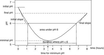
Potential information carried by graphical representation of the pH post-prandial evolution (Figure 1) was summarized by spotting or calculating the following parameters:
Generic curve of pH and potential pH variables.

• initial pH value, at feeding time (pH0);
• final pH value, 8 h after the meal (pH8);
• minimal pH value for the considered period (pHmin);
• maximal pH value for the considered period (pHmax);
• mean pH: the arithmetic average of the pH values, using both measured and interpolated values;
• standard deviation (s.d.) of pH, calculated from the same series of values as mean pH (pHs.d.);
• area under the curve (a.u.c.), represents the whole area between the pH curve and the time axis, measured in pH × h;
• amplitude of pH perturbation: ΔpH0–min = pH0−pHmin;
• decrease of pH, 8 h after feeding time: ΔpH0–8 = pH0−pH8;
• period when pH is less than a pH threshold, measured in h (time under threshold or t < pHi);
• area between the pH threshold and the pH curve, when the pH value is less than a pH threshold, measured in pH × h (area under threshold or a < pHi).
Although the proposed pH thresholds vary considerably (from 5.0 to 6.3) in the literature, only the most relevant (having biological significance) and frequently used were selected in this study: 5.5, 5.8, 6.0, 6.2. Thus, in vitro trials revealed that pH below certain levels would significantly impair or inhibit some rumen functions such as cellulose or microbial proteosynthesis (Shriver et al., Reference Shriver, Hoover, Sargent, Crawford and Thayne1986; Slyter and Rumsey, Reference Slyter and Rumsey1991; Russell and Wilson, Reference Russell and Wilson1996). In vivo trials also confirmed the influence of pH on microorganisms (Mould et al., Reference Mould, Orskov and Mann1983; Martin and Michalet-Doreau, Reference Martin and Michalet-Doreau1995).
For calculation of time and area under thresholds, it was assumed that pH evolutions within 30 min were linear (Pereira and Armentano, Reference Pereira and Armentano2000). Limitation of the studied period to 8 post-prandial hours caused supplementary truncation of some of the threshold-related variables, especially when the threshold was high. Thus, in our database, 3% of t < pH6.0 values and 14% of the t < pH6.2 values were truncated at 8 h, as an artifact linked to the limitation of the studied period. The truncated values were discarded from the analyses.
Calculation of pH variables issued from the modelling of pH graphics
As the pH curves generally exhibited a concave asymmetric shape (Figure 1), a third-degree polynomial model was regressed to all series of pH data:

The PROC REG procedure of SAS (SAS version 8.1, 1999) was used to fit polynomial equations to each of the pH datasets corresponding to the 219 pH graphics. All four coefficients (a, b, c, d) were taken into account, even if they were statistically not significant in the model. For each pH dataset, the number of measurements, the residual s.d. of the model and the s.d. of the four coefficients were also retained for further statistical analysis.
The four coefficients were used to calculate four other pH variables that cannot be directly derived from the observed pH graphics (Figure 1):
• rate of pH change at 0, 2 : 30 and 8 h, in pH units/hour (called initslope, 2 : 30 slope and finslope, respectively);
• time when pH reaches its minimum, measured in hours (t min).
Rates of pH change (dpH/dt) were obtained by considering t = 0, 2.5 or 8, respectively, in the first derivatives of polynomial equations. t min was calculated by choosing one of the two roots of derivative, depending on the sign of the first derivative. In some cases t min was outside the studied area (0 to 8 h), it was then considered equal to 8 h.
Statistical analysis
Principal component (PC) analysis was applied to the 17 post-prandial pH values in order to cluster the 219 pH graphics. Global, across- and within-study relationships between pairs of pH variables were studied. Global correlations considered the 219 observations as a whole, irrespective of the study conditions, whereas across-study considered the experiment as an explanatory factor. Pearson correlations were calculated and, when appropriate, within-study regression equations were fitted (SAS version 8.1, 1999; Minitab 13.20, 2000).
Results and discussions
Principal component analysis of pH curves
Principal component analysis allows transformation of a number of possibly correlated variables into a smaller number of uncorrelated variables, called principal components. The first principal component accounts for as much of the variability in the data as possible, and each succeeding component accounts for as much of the remaining variability as possible. This multivariate approach allowed summarizing the 17 pH values composing the pH curves (pH0, pH0 : 30, pH1, ..pH8) into few independent new variables extracting the major variations of data. The principal components with the four highest eigen values were considered for interpretation, on the basis of the main factors that characterize the pH curves: their average, slope, deepness and possible asymmetry (presence of a lag time).
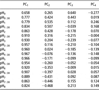
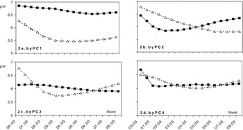
The first principal component (PC1) had the greatest weight as it accounted for 78.1% of data variability. Correlations between PC1 and the 17 pH values composing the pH curves were high and exhibited the same sign (Table 1). This expressed the influence of a ‘size factor’ and it was consistent with the fact that the 17 pH values were largely auto-correlated (data not shown). This suggests that mean pH is closely related to PC1, as also illustrated in Figure 2a, with the graphical representation of the pH curves that were the most discriminated at the two extreme parts of this principal component (average of 25 graphics for each part). The types of curves discriminated by mean pH, which is an expression of PC1, confirmed that this is an indicator of the level of rumen fluid acidity.
Global correlations between the principal components of variance and the 17 values composing the pH graphics

PC1, PC2, … = principal component 1, 2, … .
pH0, pH0 : 30, … = pH variables corresponding to pH at 0 h, 30 min, … .
Types of curves discriminated by the first four principal components of variance (PC1 to PC4) (one line represents 25 kinetics, corresponding to either maximum or minimum of the concerned principal component).

The three other principal components were also investigated in order to establish pH variables that may be complementary to mean pH. The second principal component (PC2) accounted for 12.5% of data variability. Data presented in Table 1 indicate that the extreme times of the pH graphics presented opposite signs of correlation with PC2. This suggests that PC2 mainly reflects the overall slope of pH change. This trend is illustrated in Figure 2b with the evolution of the 50 curves that were the most discriminated at the two extreme parts of the PC2. It must be stressed that for the decreasing pH curves, pHmin was frequently achieved beyond 8 h, whereas, for the increasing type, pHmin occurred more early.
The third principal component (PC3) accounted for 5.5% of the variability. Table 1 indicates that the initial and final phases of the pH graphs have an opposite sign with the middle phase on PC3. This suggests that pH curves were mainly discriminated by their relative ‘deepness’. Figure 2c, built from the 50 pH graphics most differentiated by PC3, exhibited that fact with flat-shaped curves opposite to deep ones, which suggested a stronger perturbation. It has to be noticed that the flat type of curves rarely reached their minimum within 8 h.
The fourth principal component (PC4) accounted for only 1.7% of data variability and suggested the existence of an asymmetry of curves. Indeed, graphical expression for the 50 pH curves mostly differentiated by this principal component shows the existence of two opposite groups: pH curves with an initial ‘lag-time’ v. pH curves that decrease immediately and fairly abruptly, quickly reaching their minimum pH (Figure 2d). Moreover, the final slope was higher for the pH curves that began with a lag.
Repartition of the 219 treatments on the four principal components was globally homogenous, suggesting a certain ‘continuum’ in the data according to the diversity of the pH graphics. To evaluate the weight of the across- and within-study variations on the determination of the components, an analysis of variance was applied on the values of the treatments on the four first principal components. The influence of the publication was highly significant for the four principal components with corresponding F ratios of 8.0, 10.2, 9.9 and 7.3. These comparable values obtained for the Fisher ratios suggest that the relative weight of among- and within-study was consistent from one principal component to another. Moreover, the residual variations of the four analyses of variance were normally distributed and, logically, they were not mutually correlated between the four principal components.
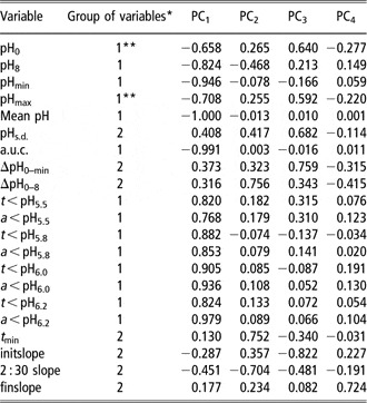
Based on their global correlations with principal components (Table 2), the pH variables were clustered in two groups. In Group 1, mean pH, a.u.c., pHmin, pH8 and the eight threshold-related variables are largely explained by the first principal component of variance (0.77 < r < 1.00); in contrast, they are weakly correlated to PC2, PC3 and PC4 (0.00 < r < 0.47). The variable pHmax and, in the same manner, pH0 were partly discordant with Group 1: their correlations with PC1 are weaker than those of the above-mentioned pH variables (r = 0.708 and 0.658, respectively). Moreover, they were moderately related to PC3 (r = 0.592 and 0.640, respectively).
Global correlations between the principal components of variance and the pH variables

a.u.c. = area under the curve.
*Group 1 = mostly related to PC1; Group 2 = mostly related to PC2.
**Partly discordant with the rest of Group 1.
In Group 2, variables expressing pH fluctuations (ΔpH0–min, ΔpH0–8 and pHs.d.) and variables issued from modelling the pH graphics (t min, initslope, 2 : 30 slope and finslope) were poorly correlated with PC1 (0.13 < r < 0.45); on the contrary, they exhibited much higher correlations with one of the other principal components. Thus, ΔpH0–8, t min and 2 : 30 slope were mostly related to PC2 (r = 0.756; 0.752 and 0.704, respectively), initslope, ΔpH0–min and pHs.d. were mostly related to PC3 (r = 0.822; 0.759 and 0.682, respectively) and the final slope was mostly related to PC4 (r = 0.724).
Group 1: pH variables strongly correlated to PC1
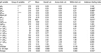
Mean pH (Table 3) had a relatively low average (6.13 ± 0.018) across the 219 treatments, and a normal distribution (of an Anderson–Darling index of 0.59) with a slight left asymmetry (0.19). Most authors in the database calculated arithmetic and not weighted average; when measurement times were unevenly distributed over the studied period (67% of the cases), this induced biases as also observed by Murphy (Reference Murphy1981) and by Pitt and Pell (Reference Pitt and Pell1997).
Variability and distribution of pH variables describing the pH graphics

a.u.c. = area under the curve.
*Variable with a normal distribution (Anderson–Darling test); s.d. = standard deviation.
**Where n < 219, values were calculated from non-truncated values.
***Partly discordant with the rest of Group 1.
Our database revealed an underestimation of mean pH that was small (0.04 pH units on average) but variable (s.d. of 0.05 pH units and biases up to 0.28 pH units). Biases have little influence on within-study comparisons but induce further biases when analyzing data from different trials, e.g. in meta-analyses or rumen modelling. However, irrespective of the accuracy of its calculation, the mean pH alone does not offer information on pH pattern throughout the day. Moreover, the s.d., which could have brought supplementary information, is rarely reported.
Area under the pH curve (a.u.c.) averaged 48.9 ± 0.15 pH units × hours and showed a normal distribution, similar to mean pH (Table 3). This variable is sometimes reported as a descriptor of the ruminal pH evolution (Yang et al., Reference Yang, Beauchemin and Rode2000 and Reference Yang, Beauchemin and Rode2001) but in fact it has no other value than being a slightly more precise way to express mean pH when unevenly spaced measurements are used: by calculating the a.u.c. and by dividing it to time units, a more accurate mean is obtained. As in the present study, mean pH was calculated from all pH values (at 30-min intervals) not only from measured values, the corresponding a.u.c. brought no supplementary information and was discarded from further analysis.
Of the 17 values composing the pH graphics, four were investigated as having possible significance in describing pH evolution: pH0, pHmax, pHmin and pH8 (Table 3). Some information can be drawn when pHmax occurs later than t0 (14% of the cases in our database) or when these values are much different from pH thresholds. For example, in our database, pHmax was lower than 6.2 in 34 cases, suggesting that the ruminal digestion (e.g. cellulolysis) of concerned animals was impaired. pHmax and pHmin are sometimes proposed besides mean pH as supplementary quantitative descriptors of the ruminal status (Beauchemin and Buchanan-Smith, Reference Beauchemin and Buchanan-Smith1990; Maekawa et al., Reference Maekawa, Beauchemin and Christensen2002) but these variables rely on punctual measurements. This makes them subject to bias as a result of the sampling schedule chosen.
Within Group 1, mean pH, a.u.c., pHmin and pH8 have a distinct behaviour, because of their very low global, across- and within-study s.d.s (Table 3). They might be less sensitive to the influence of dietary factors affecting rumen acidity (concentrate proportions from 0% to 100%, starch content of diets from 0% to 75.7% – DM basis; NDF content from 14.7% to 65.0% – DM basis, total tract digestibility of starch from 66% to almost 100%, etc.).
‘Threshold-related’ pH variables, time under threshold and area under threshold are also highly correlated with PC1. These variables are claimed to have higher biological significance than mean pH. However, a major limitation in the use of threshold-related variables was their truncation at 0, which occurred in our study when the threshold value was lower than pHmin. Throughout the 219 treatments, even for the highest of the studied thresholds (pH = 6.2), many of the corresponding values were equal to 0 (30% for t < pH6.2 and 15% for a < pH6.2). Also, truncation at 8 h occurred as a result of the chosen period of 8 post-prandial hours. All truncated values were eliminated from the statistical analysis in this study; therefore, data in Table 3 are based on non-truncated values.
Truncation was in general accompanied by a non-normal distribution of threshold-related variables (Table 3). The cause of this distribution is that, due to the general pattern of pH, area under pH 5.5, 5.8, 6.0 and 6.2 decreased asymptotically to 0 while the mean pH became higher than the pH threshold.
Therefore, caution should be taken when using linear models for statistical analysis that includes threshold-related variables. Different from mean pH, the eight threshold-related variables showed much higher variability, which increased with the level of threshold (Table 3).
Group 2: pH variables weakly correlated to PC1
ΔpH0–min; ΔpH0–8 and pHs.d. showed large variability (Table 3), which could make them good candidates as descriptors of changes in rumen status when trying to relate them to diet characteristics. However, ΔpH0–8 and ΔpH0–min have the disadvantage of being based on punctual measurements of pH; thus they are subjected to errors. In our database, pHs.d. varied strongly, from 0.02 to 0.63 pH units, when only measured points, as in published trials, were used to calculate it. The utility of this variable is impaired because it carries limited information (it expresses the extent of pH variation without detecting its trend). Various authors mention differences between pH values or use the concept of pH fluctuations in commentaries (Malestein et al., Reference Malestein, Van’t Klooster, Pains and Connette1984; MacLeod et al., Reference MacLeod, Colucci, Moore, Grieve and Lewis1994; Pitt and Pell, Reference Pitt and Pell1997) but these were not translated into explicit quantitative pH variables.
The variables initslope, 2 : 30 slope, finslope and t min, were calculated from coefficients obtained by regression of the pH curves with a third-degree polynomial equation. The equation was chosen on the basis of the general shape of the pH graphics (Figure 1) and of the types of pH curves discriminated by the first four principal components (Figure 2). This choice compromised between the need to fit accuracy and the need to interpret the equations coefficients. Although part of the pH curves tended to be rather linear during the 8 h after the meal, the use of a complete type of third-degree polynomial fitting was decided in order to provide a full table of regression coefficients. Of the 219 regressions, 98% were significant; on the other hand, in 40% of the cases coefficients of t 2 and t 3 were not significant. Nevertheless, we intended to use a single approach; hence, all equations and all coefficients were retained for further calculations. Effectively, the cubic equation presented flexibility that allowed to conveniently describe the various shapes of pH curves, including the quasi-linear ones.
The initial and final slopes of pH evolution (initslope, finslope) are expressions of pH rates of decrease and recovery, respectively. However, the initial slope was insufficient to describe pH decrease: pH was not measured at t0 in 13% of the treatments, and some of the pH curves tended to increase for a while after t 0. Therefore, pH slope at t 2.5 (2 : 30 slope), in the middle of the t 0–t min interval, was considered more appropriate to describe pH decrease, whereas the initial slope was retained as an identifier of pH curves expressing a lag before decrease.
In the literature, the coefficients from fitting the polynomial equation were sometimes directly used for statistical comparisons of the values composing pH graphics (Leiva et al., Reference Leiva, Hall and Van Horn2000). On the contrary, the rates of pH change and t min are seldom used in the literature and, to our knowledge, no attempt was made to use them in analysis of data from the literature.
The concepts of pH decrease and recovery were used, without being quantified, by several authors (Malestein et al., Reference Malestein, Van’t Klooster, Pains and Connette1984; Pitt and Pell, Reference Pitt and Pell1997; Leiva et al., Reference Leiva, Hall and Van Horn2000), some of them suggesting possible relationships with ruminal processes. Sometimes, the time when pH reaches its minimum (t min) is briefly used in text commentaries (Khalili and Huhtanen, Reference Khalili and Huhtanen1991; Krause et al., Reference Krause, Beauchemin, Rode, Farr and Nørgaard1998). Only in two recent references (Krause and Combs, Reference Krause and Combs2003; Krause et al., Reference Krause, Combs and Beauchemin2003) it was found as an explicit variable used to support the hypothesis on ruminal digestion. Pitt and Pell (Reference Pitt and Pell1997) reported that t min could be reasonably predicted within the net carbohydrate and protein system (from DMI, eNDF and the concentration of organic acids in the rumen). However, it has to be mentioned that efficacy of t min is highly dependent of the frequency of pH measurements.
All variables of Group 2 (ΔpH0–min; ΔpH0–8, pHs.d., initslope, 2 : 30 slope, finslope, t min) expressed large variability (Table 3). Besides, their high correlations with PC2, PC3 and PC4 and low correlations with PC1 (Table 2) make them good candidates as descriptors of changes in the rumen status.
Correlations among pH variables
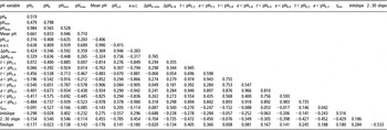
As a consequence of their high correlations with PC1, the global correlations among pH variables from Group 1 were high (Table 4). The across-study and within-study correlations showed the same trend (data not shown). The high correlations between the mean pH and pHmin, pHmax, pH0 or pH8 were determined by the auto-correlation of the 17 values composing the pH graphics (as shown by their relationships with PC1). The auto-correlative process also explains the weaker correlations between pHmax (or pH0) and the above-mentioned variables: correlations between distant values are weaker, especially at the beginning of the data series.
Global correlations among pH variables

a.u.c. = area under the curve.
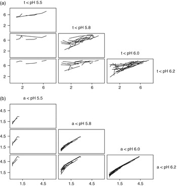
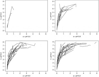
The global mutual correlations were systematically high among the four areas under threshold variables; they were also significant but lower for the four variables time under threshold (Table 4). This could be determined by the limitation of the studied period to 8 h, which has induced the non-linearity, more stressed for time under threshold than for the area under threshold variables (Figure 3). This is also expressed by the relationships between time and area under the same threshold (Figure 4).
Relationships among threshold-related variables describing pH curves. (a) Time under threshold variables (periods while pH is lower than 5.5, 5.8, 6.0 and 6.2), in hours. (b) Area under threshold variables (areas between the line representing pH = 5.5, 5.8, 6.0, 6.2 and the pH curve), in hours × pH units.

Relationships between time under threshold and area under the same threshold.

Also, high global correlations linked threshold-related variables and mean pH (Table 4). Beauchemin et al. (Reference Beauchemin, Yang and Rode2003) found much lower correlations between mean pH and time under pH 5.8 or area under pH 5.8, but they used fewer observations, from a single study. It is noteworthy that they used continuous measuring of ruminal pH, whereas our study is mostly based on measurements with time intervals of more than 30 min. These relationships are detailed in Figure 5. The graphical encoding showed that the global-, among- and within- relationships followed approximately the same trends and it also expressed the above-mentioned ‘asymptotic’ evolutions of the threshold-related pH variables. Generally, global correlations were higher than across-study correlations, which were higher than within-study correlations (0.89, 0.83 and 0.69, respectively, when only significant correlations were considered). This suggests that threshold-related variables may be interesting as substitutes of mean pH, especially for within-study variations (e.g. for studying feed characteristics).
Relationships between mean pH and threshold-related parameters (values of threshold-related parameters that are equal to 0 or 8, as a result of the studied period chosen, were excluded from analyses).

Mean pH and pHmin presented a similar level and pattern of correlations with threshold-related variables. On the contrary, correlations between the threshold-related variables and pH0, pH8, pHmax, pHs.d., ΔpH0–min and ΔpH0–8 were moderate and even insignificant as the threshold value decreases.
Strong global, across- and within-study relationships between mean pH and other variables from Group 1 imply that mean pH can be replaced by any of them as descriptor of rumen status. Of these, threshold-related variables offer the advantage of biological significance, as the deleterious effects of the low pH depend on the duration and intensity of its decrease (Beauchemin, Reference Beauchemin1991; Krehbiel et al., Reference Krehbiel, Britton, Harmon, Wester and Stock1995; Nocek et al., Reference Nocek, Kautz, Leedle and Allman2002).
Relationships among variables from Group 2 were more heterogeneous as they were related to more than one principal component. High global correlations between pHs.d. and the pH drop, expressed by either ΔpH0–min or ΔpH0–8, confirmed the fact that pHs.d. offers a good image of pH stability in the rumen (Table 4). In fact, the three variables behaved in the same manner regarding their correlations with the principal components (Table 2), their variability (Table 3) and their inter-correlations (Table 4).
Moderate correlations were detected between t min and initial slope (0.516) or slope at 2 : 30 h (−0.429). A negative moderate correlation (−0.533) also linked the final slope with the slope at 2 : 30 h (Table 4). The other correlations between variables issued from modelling were weak (r < 0.28), which implies they may be complementary in expressing pH evolution.
Global correlations between ΔpH0–min, ΔpH0–8 or pHs.d. and the pH slope at 2 : 30 h were high (r > 0.70); their correlations with the initial slope or t min were rather inconsistent and their correlations with the final slope were weak (r < 0.14). However, the low correlations of the final slope with other variables may be due to the fact that PC4 is insufficiently expressed in pH curves described by few measurements. The values of t min were higher for curves presenting high values of ΔpH0–8 and low values of pH8 (Table 4). The drop ΔpH0–min was not related to t min but was closely linked to the slopes at t 0 and t 2.5, which seems logical. These two slopes were also positively related to pHmin and negatively to pHs.d. (Table 4).
Conclusions
The relationships between pH variables and the principal components allowed splitting the pH variables that are linked to PC1 (Group 1) and to PC2, or PC3 or PC4 (Group 2). Screening the relevant variables only, this clustered the mean pH or threshold-related variables to pHs.d. and the pH calculated from the regression equations, such as the rates of pH decreasing or t min.
As the principal components are independent by definition, the two groups of pH variables may be complementary in describing post-prandial ruminal pH evolution. This is consistent with the weak correlations (r < 0.40) between any of the variables from Group 1 and those from Group 2, except for the slope at 2 : 30 h.
Of the variables belonging to Group 1, a.u.c., pHmin and pH8 variables have lower relevance as reliable descriptors of rumen pH. On the contrary, threshold-related variables might carry supplementary information about pH dynamics induced by diet characteristics, since they are calculated only from pH values that are relevant to ruminal fermentation and their within-study correlations with mean pH are rather moderate (0.69, on average). However, in our database, which is representative of normal feeding situations, these variables were truncated and showed distributions other than normal, irrespective of the choice of pH threshold. This implies that caution should be taken when they are used as descriptors of ruminal pH evolution, e.g. in meta-analyses or rumen modelling.
The pH slope variables (at 0, 2.5 and 8 h), t min, ΔpH0–min, ΔpH0–8 and pHs.d. expressed fairly similar relationships with the principal components of variance (poorly correlated to PC1, highly correlated to PC2, PC3 and PC4). However, the pH slope variables and t min are more reliable than ΔpH0–min or ΔpH0–8, the latter being determined from only two measurements. Moreover, simple differences between the critical pH values do not take time into account. Compared to pHs.d., pH slope variables and t min offered the advantage of adding information on the nature and mean of pH irregularities.
A third-degree polynomial equation was used to describe the 0 to 8 h post-prandial pH graphics of various forms. We consider that next to pH graphics, the authors should also report the four coefficients estimates derived with this model. Besides a fairly accurate reproduction of the original curves, this would allow the calculation of new pH variables (rate of pH change, t min) or recalculation of variables, which are based on punctual measurements (e.g. pHmin). These variables may be used in quantitative analyses of data from the literature. These new variables are poorly related to the currently used mean pH or threshold-related variables, which means they carry additional information on pH variation; this makes them good candidates as descriptors of short-term ruminal status.
Implications
The evolution of the ruminal pH in the first 8 h after the morning meal can be conveniently modelled by a third-degree polynomial equation whose coefficients allow (either directly or through derived pH variables) the quantitative comparison of various pH graphics and quantitative reviews across published data. The analysis of variables summarizing post-prandial evolution of ruminal pH revealed that some of them could replace or complement the classical mean pH, as descriptors of short-term ruminal acidity.